Microscopic dynamics and Bose-Einstein condensation in liquid helium

Abstract

We review fundamental problems involved in liquid theory including both classical and quantum liquids. Understanding classical liquids involves exploring details of their microscopic dynamics and its consequences. Here, we apply the same general idea to quantum liquids. We discuss momentum condensation in liquid helium which is consistent with microscopic dynamics in liquids and high mobility of liquid atoms. We propose that mobile transit atoms accumulate in the finite-energy state where the transit speed is close to the speed of sound. In this state, the transit energy is close to the zero-point energy. In momentum space, the accumulation operates on a sphere with the radius set by interatomic spacing and corresponds to zero net momentum. We show that this picture is supported by experiments, including the measured kinetic energy of helium atoms below the superfluid transition and sharp peaks of scattered intensity at predicted energy. We discuss the implications of this picture including the macroscopic wave function and superfluidity.

1 Introduction

Problems involved in liquid theory are fundamental. As discussed by Landau, Lifshitz and Pitaevskii (LLP), these problems include (a) strong interatomic interactions combined with dynamical disorder and (b) the absence of a small parameter Landau and Lifshitz (1970); Pitaevskii (1994). For this reason, no general theory of liquids was long thought to be possible, in contrast to theories of solids and gases. For example, calculating generally-applicable thermodynamic properties such as energy and heat capacity as well as their temperature dependence form essential part of theories of solids and gases. Deriving such general relations was considered impossible in liquids Landau and Lifshitz (1970); Pitaevskii (1994).

The first part of the problem stated by LLP can be illustrated by writing the liquid energy as

$$E=\frac{3}{2}NT+\frac{n}{2}\int g(r)u(r)dV$$ (1)

where $n$ is concentration, $g(r)$ is the pair distribution function, $u(r)$ is the interaction potential, interactions and correlations are assumed to be pairwise and $k_{\rm B}=1$.

Early liquid theories Kirkwood (1968); Born and Green (1946); Zwanzig (1954); Barker and Henderson (1976) considered that the goal of the statistical theory of liquids is to provide a relation between liquid thermodynamics and liquid structure and intermolecular interactions such as $g(r)$ and $u(r)$ in Eq. (1). Working towards this goal involved developing the analytical models for liquid structure and interactions, which has become the essence of these theories Kirkwood (1968); Born and Green (1946); Zwanzig (1954); Barker and Henderson (1976); Egelstaff (1994); Faber (1972); March (1990); March and Tosi (1991); Tabor (1993); Balucani and Zoppi (2003); Barrat and Hansen (2003); Hansen and McDonald (2013). The problem is that the interaction $u(r)$ in liquids is both strong and system-specific, hence $E$ in Eq. (1) is strongly system-dependent as stated by LLP. For this reason, no generally applicable theory of liquids was considered possible Landau and Lifshitz (1970); Pitaevskii (1994). An additional difficulty is that interatomic interactions and correlation functions are generally not available apart from fairly simple model liquids and can be generally complex involving many-body, hydrogen-bond interactions and so on. This precludes calculation of the liquid energy in the approach based on Eq. (1) or its extensions involving, for example, higher-order correlation functions Born and Green (1946); Barker and Henderson (1976). Even when $g(r)$ and $u(r)$ are available in simple cases, the calculation involving Eq. (1) or similar is not enough: in order to explain experimental temperature dependence of energy and heat capacity of real liquids Trachenko and Brazhkin (2016); Wallace (1998, 2002); Proctor (2020, 2021); Chen (2022), one still needs to develop a physical model in this approach.

Common liquid models are inapplicable to understanding the energy and heat capacity of real liquids. These models include the widely discussed Van der Waals model, the hard-spheres model and their extensions Barrat and Hansen (2003); Ziman (1979); March (1990); Parisi and Zamponi (2010). Both models give the specific heat $c_{v}=\frac{3}{2}k_{\rm B}$ Landau and Lifshitz (1970); Wallace (1998, 2002), the ideal-gas value, in contrast to experiments showing liquid $c_{v}=3k_{\rm B}$ close to melting Wallace (1998, 2002); Proctor (2021). These models were also used as reference states to calculate the energy (1) by expanding interactions into repulsive and attractive parts (see, e.g., Refs. Barker and Henderson (1976); Weeks et al. (1971); Chandler et al. (1983); Zwanzig (1954); Rosenfeld and Tarazona (1998)). These parts understandably play different roles at high and low density, however this method faces the same problem outlined by LLP: the interactions and expansion coefficients are strongly system-dependent and so are the final results, precluding a general theory.

In solids, both crystalline and amorphous, the above issues do not emerge because the solid state theory is based on collective excitations, phonons. This theory is predictive, physically transparent and generally applicable to all solids. There is no need to explicitly consider structure and interactions in order to understand basic thermodynamic properties of solids. Most important results such as universal temperature dependence of energy and heat capacity readily come out in the phonon approach to solids Landau and Lifshitz (1970).

The simplifying small parameter in solids is small phonon displacements from equilibrium, but this seemingly does not apply to liquids because liquids do not have stable equilibrium points that can be used to sustain these small phonon displacements. Weakness of interactions used in the theory of gases does not apply to liquids either because interactions in liquids are as strong as in solids. This constitutes the second, no small parameter problem, outlined by LLP.

Working towards solving the liquid theory problem involved several steps. The important first step involved the consideration of microscopic dynamics of liquid particles provided by the Frenkel theory Frenkel (1947): differently from solids where particle dynamics is purely oscillatory and gases where dynamics is purely diffusive, particle dynamics in liquids is mixed and combines oscillations around quasi-equilibrium points as in solids and diffusive motions between different points. This consideration led to understanding collective excitations in liquids, phonons, with an important property that the phase space available to these phonons is not fixed as in solids but is instead variable Trachenko and Brazhkin (2016); Proctor (2020, 2021); Chen (2022). In particular, this phase space reduces with temperature. This effect has a general implication: specific heat of classical liquids universally decreases with temperature, in agreement with experiments Trachenko and Brazhkin (2016); Proctor (2020, 2021) (in molecular liquids, a competing increase of $c_{v}$ at high temperature may be related to progressive excitations of internal molecular degrees of freedom - this mechanism is also present in quantum solids and is unrelated to liquid physics). This effect also addresses the no small parameter problem stated by Landau, Lifshitz and Pitaevskii: the small parameter exists in liquids but it operates in a variable phase space.

The above theory is closely based on details of microscopic particle dynamics in liquids. This was essential to understand classical liquids. In this paper, we explore the implications of microscopic dynamics in quantum liquids. There is a good reason for doing this: a microscopic theory requires microscopic dynamics. For example, understanding superconductivity is aided by its microscopic theory Bardeen et al. (1957). In contrast, no microscopic theory of liquid helium ⁴He and its superfluid properties is considered to exist, as noted by several observers. For example, Pines and Nozieres observe Pines and Nozieres (1999) that “microscopic theory does not at present provide a quantitative description of liquid He II” (“II” here refers to helium below the superfluid transition temperature $T_{\lambda}=2.17$ K), adding that a microscopic theory exists only for models of dilute gases or models with weak interactions where perturbation theory applies such as the Bogoliubov theory. Griffin similarly remarks that we can’t make quantitative predictions of superfluid ⁴He on the basis of existing theories and depend on experimental data for guidance, and attributes theoretical problems to the “difficulties of dealing with a liquid, whether Bose-condensed or not” Griffin (1993). Pines, Nozieres, Griffin and other authors recognize that the same fundamental theoretical problems outlined by LLP and related to strong interactions combined with dynamical disorder apply to both quantum and classical liquids.

In view of this, progress in the field is likely to come from discussing microscopic details of liquid helium and particle dynamics in particular. This dynamics is a starting point of our discussion.

In liquid helium, atoms are located in the range of the strong part of the potential and close to its minimum as follows from, for example, pair distribution function Ceperley (1995). Since the early work of Frenkel, we know the key element of microscopic dynamics in such a liquid at low temperature: each particle oscillates around quasi-equilibrium position in a “cage”, followed by the diffusive jump to the neighbouring position Frenkel (1947). Path integral simulations show minima of the velocity autocorrelation function below $T_{\lambda}$ in liquid helium Nakayama and Makri (2005), indicating the presence of the oscillatory component of particle motion Cockrell et al. (2021). The oscillations are interrupted by diffusive atomic jumps separated in time by liquid relaxation time $\tau$ Frenkel (1947). Seen in molecular dynamics simulations and referred to as “transits” Wallace et al. (2001), these mobile atoms give liquids their ability to flow. This applies to both classical and quantum liquids.

This oscillatory-transit dynamics consistently explains dynamical and thermodynamic properties of liquids Frenkel (1947); Dyre (2006); Trachenko and Brazhkin (2016); Proctor (2021). Once considered in liquid helium, this dynamics presents a problem for understanding Bose-Einstein condensation (BEC), as follows.

Understanding liquid ⁴He involved exciting new ideas including attributing superfluidity to the BEC in zero momentum state $p=0$ where only about 10% of atoms are in the condensate Pines and Nozieres (1999); Griffin (1993); Ceperley (1995); Pitaevskii and Stringari (2016); Annett (207); Leggett (2008); Glyde (2018); Balibar (2017). The experimental evidence for this is not unambiguous (see, for example, Ref. Prisk et al. (2017), p. 175 and cited references therein as well as discussion in Sections 2.2 and 2.3), however there is also an issue related to microscopic dynamics. In gases, BEC understandably corresponds to the immobile state $p=0$ at low temperature. Liquids are importantly different because every atom in the liquid necessarily possesses high mobility at any temperature: an atom either oscillates with the ever-present component of zero-point motion (this motion is particularly important in liquid ⁴He Annett (207)) or becomes a mobile diffusive transit Frenkel (1947); Dyre (2006); Wallace et al. (2001); Proctor (2021). As in solids, the oscillatory atoms do not undergo the BEC. This leaves the flow-enabling transits as the remaining sub-system where BEC can possibly operate. However, transits are inherently mobile and, moreover, strongly and constantly interact with surrounding mobile atoms. Depending on the dynamical regime, these surrounding mobile atoms are either (a) both oscillatory and other mobile transit atoms in the low-temperature oscillatory-transit regime of liquid dynamics or (b) mobile transit atoms in the high-temperature diffusive regime where the oscillatory component of motion is lost and all atoms become mobile transits Cockrell et al. (2021); Proctor (2021). An atom in the condensate at $p=0$ can not remain immobile while strongly and constantly interacting with surrounding mobile atoms. Assuming 10% of atoms in the immobile $p=0$ state would imply that each immobile atom interacts with about 10 of its nearest-neighbour mobile atoms on average, with the interaction strength comparable to that in solids. This is not possible. One could try to imagine that 10% of atoms in the state $p=0$ are organised in clusters and hence are not affected by interactions with mobile atoms. However this would apply to the bulk of the cluster only, whereas atoms at the surface of the cluster would still be excited by interactions with surrounding mobile atoms.

A somewhat related problem with BEC at $p=0$ in liquid helium was noted in the early studies of superfluidity by Landau Landau (1941): nothing prevents atoms in BEC at $p=0$ to collide with excited atoms, leading to friction and hence no superfluidity. This problem was later described in terms of condensate depletion due to interactions Griffin (1993), however it was not demonstrated that this depletion cannot be complete (see, e.g., p. 175 of Ref. Prisk et al. (2017)) as discussed in more detail below.

This concludes our longer-than-usual introduction. This was needed to put liquid helium in the wider context of a more general liquid research and liquid problem. This discussion leads us to look for a way to discuss liquid helium which is consistent with microscopic liquid dynamics and high atomic mobility.

In this paper, we discuss BEC in liquid helium which is consistent with microscopic dynamics in liquids and high mobility of liquid atoms in particular. We propose that a large number of transits accumulate in the finite-energy state where the transit speed is close to the speed of sound. In this state, the transit energy is close to the zero-point (vacuum) energy. In momentum space, the accumulation operates on a Bose-liquid sphere with the radius set by interatomic spacing and corresponds to zero net momentum. We show that this picture is supported by experiments, including the measured kinetic energy of helium atoms below the superfluid transition and sharp peaks of scattered intensity at predicted energy. We discuss the implications of this picture including the macroscopic wave function and superfluidity.

2 Results and discussion

2.1 Transit dynamics

Mobile transit atoms are relevant to superfluidity because they enable liquid flow and set its properties. At fixed cage volume, a transit involves surmounting large energy barrier due to steep interatomic repulsion and hence very long waiting times. Instead, the transit is enabled by temporary increase of the cage volume due to fluctuations, thermal or quantum, as proposed by Frenkel Frenkel (1947) and widely appreciated since Dyre (2006). This is illustrated in Figure 1: when neighbouring atoms move out of the way, the transit to the neighbouring cage takes place where the oscillation resumes until the next transit, and so on.

The transit is a quantum-mechanical object: the de Broglie wavelength at 4 K where helium condenses is about 4 Å, and is larger than the interatomic separation Annett (207). To write the wavefunction of the transit, we consider its translational motion between two quasi-equilibrium positions in Figure 1. The transit is a fast process lasting during the shortest time scale in the system close to the Debye vibration period, $\tau_{\rm D}$ Frenkel (1947); Dyre (2006). The potential $V(x)$ acting on the transit from surrounding particles can be assumed as slowly-varying during the fast transit process so that the Wentzel–Kramers–Brillouin approximation applies:

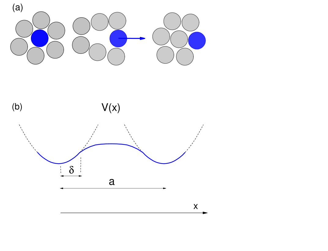
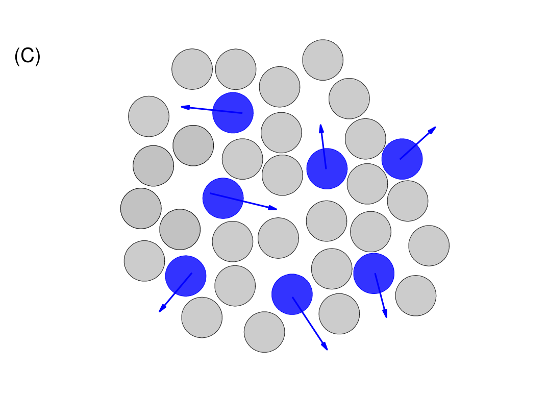
Figure 1: (a) A mobile transit showing the diffusive atomic motion between two quasi-equilibrium oscillatory states when the cage opens up due to fluctuations. (b) Potential experienced by the atom in the oscillatory and transit states. (c) A set of transit atoms in a liquid. Schematic illustration.

$$\begin{split}&\psi(x)=\frac{1}{\sqrt{k(x)}}\exp\left(i\int\limits^{x}k(x)dx\right)\\ &k(x)=\left(\frac{2m}{\hbar^{2}}\left(E-V(x)\right)\right)^{\frac{1}{2}}\end{split}$$ (2)

where $\psi(x)$ is the wavefunction of the transit and $E$ is the transit energy.

Approximating the slowly-varying potential experienced by the transit by a constant gives the plane wave with constant $k$: $\psi(x)\propto\exp\left(ikx\right)$. This wave function continuously joins the oscillatory wavefunctions of the atom in the oscillatory states before and after the transit. An example of a quantum-mechanical model of the oscillatory-transit dynamics with continuous solutions in space and time is shown in the Appendix.

We now make the key observation regarding the absolute value of transit momentum ${\bf p}_{t}$, $p_{t}=|{\bf p}_{t}|$. For a large number of atoms, $p_{t}$ is not arbitrary but is set by liquid structure and dynamics. The transit speed can be estimated as $v=\frac{\Delta x}{\Delta t}$, where $\Delta x$ is the distance travelled by the transit and $\Delta t$ is the transit time. $\Delta x$ is close to the interatomic separation in the liquid, $a$ (the “UV” cutoff in condensed matter). $\Delta t$ is set by atom inertia and the shortest time scale in the system comparable to the Debye vibration period $\tau_{\rm D}$. The mean value of $v$ (mean in a sense of $\Delta x$ fluctuating around $a$ and $\Delta t$ fluctuating around $\tau_{\rm D}$) is $v=\frac{a}{\tau_{\rm D}}$ or $v=a\omega_{\rm D}$, where $\omega_{\rm D}$ is the Debye frequency which is inverse of $\tau_{\rm D}$ and is close to the intra-cage rattling frequency. This ratio, $\frac{a}{\tau_{\rm D}}$, is the speed of sound, $c$. This follows from writing the dispersion relation in the linear form as $\omega=ck$, using $\omega=\omega_{\rm D}$ and Debye wavevector $k=k_{\rm D}$ and noting $\omega\approx\frac{1}{\tau_{\rm D}}$ and $k_{\rm D}\approx\frac{1}{a}$.

Hence the mean $p_{t}$ and energy $E_{t}$ of transits are close to

$$\begin{split}&p_{t}=mc\\ &E_{t}=\frac{mc^{2}}{2}=14~{}{\rm K}=0.28~{}{\rm THz}\end{split}$$ (3)

where $c=238$ m/s is calculated from the dispersion curve measured in neutron scattering experiments Pitaevskii and Stringari (2016) and $m$ is the mass of helium atom.

We note that the kinetic energy of the transit atom is comparable, by order of magnitude, to the oscillatory ground-state energy which this atom had inside the cage before the diffusive jump (the oscillatory atom is in the ground state around $\sim 1$ K because $\hbar\omega$ is about 54 K in helium Annett (207)). Using $v=a\omega$ (here and below we drop the lower index in $\omega_{\rm D}$ for brevity) for the transit as before and the uncertainty relation for the transit atom localised within the distance $a$ during the transit process as

$$mva=ma^{2}\omega\sim\hbar,$$ (4)

we see that the oscillatory energy in the ground state $E_{g}=\frac{\hbar\omega}{2}$ and the transit kinetic energy $E_{t}=\frac{mv^{2}}{2}$ become the same. This is consistent with the oscillatory-transit dynamics envisaged by Frenkel Frenkel (1947): an oscillating atom becomes a transit when cage atoms move out of the way. In this process, the energy of the transit atom is close to the kinetic energy this atom had inside the cage before the jump. Another way to see this is to note that the average kinetic energy of the oscillating atom inside the cage in the ground state, $\left<K_{g}\right>$, is one half of the ground state energy: $\left<K_{g}\right>=\frac{\hbar\omega}{4}$. Taking $\hbar\omega$=54 K Annett (207), we find $\left<K_{g}\right>$ close to $E_{t}$ in (3).

More generally, the closeness of the energy of flow-enabling liquid transits and the in-cage oscillatory energy is consistent with the increasingly appreciated similarity of liquid and solid properties and the general approach to liquids based on solidlike, rather than gaslike, concepts Wallace (2002); Dyre (2006); Trachenko and Brazhkin (2016); Proctor (2021). This similarity has remained under-explored in liquids Trachenko and Brazhkin (2016). This notably included quantum liquids where gaslike approaches were used such as the Bose-Einstein condensation at zero momentum Pines and Nozieres (1999); Griffin (1993); Pitaevskii and Stringari (2016); Annett (207); Leggett (2008).

The above closeness of the transit energy and the energy this atom had inside the cage can be used to approximately estimate the distribution of transit momenta. This closeness implies that momenta of transit atoms are close to momenta these atoms had inside the cage, $p$ (except for small $p$ as discussed below) and, consequently, that the distributions of momenta of both sets of atoms are also close. The distribution of $p$ inside the cage is set by the momentum distribution of the harmonic oscillator in the quantum regime $T\ll\hbar\omega$ in the ground state, with the probability

$$\rho\propto e^{-\frac{p^{2}}{m\hbar\omega}}$$ (5)

Large $p$ give small $\rho$. Small $p$ do not apply to transits because flow-enabling transits are highly mobile by definition. Indeed, zero momenta of transits implies the absence of liquid flow. Lets consider $\rho$ at intermediate $p$ corresponding to $p=p_{t}=mc$ in (3). Using $c=a\omega$ for the transit atom as before, the argument in the exponent becomes $\frac{ma^{2}\omega}{\hbar}$ in absolute value. This ratio is on the order of 1 in view of the uncertainty relation (4). Using $\frac{p_{t}^{2}}{2m}=14$ K and $\hbar\omega$=54 K as before, the argument in the exponent is about $-0.5$. Therefore, $\rho$ is not small, corresponding to a large number of transit atoms with momenta close to $p_{t}$. This is the case because the probability (5) is quantum. Were the probability classical and set by the thermal distribution of high-energy transits with $p=p_{t}$ as

$$\rho\propto e^{-\frac{p_{t}^{2}}{2mT}},$$ (6)

$\rho$ would be close to 0 because $\frac{p_{t}^{2}}{2m}\gg T$ at $\sim 1$ K.

We have seen that the two parameters characterising the condensed state of matter, $a$ and $\tau_{\rm D}$, constrain the speed of a large number of transits to be close to $v=\frac{a}{\tau_{\rm D}}=c$. Characteristic values of these two parameters, $a$ and $\tau_{\rm D}$, are set by fundamental physical constants Trachenko and Brazhkin (2020). As a result, $c$ is also governed by fundamental physical constants Trachenko et al. (2020). This additionally points to the physical significance of the state (3).

We now add the main proposal: BEC in liquid ⁴He corresponds to a large number of transits occupying the state with a finite momentum close to $p_{t}$ and energy $E_{t}$ in Eq. (3). The BEC at finite energy (BECFE) takes place on a sphere with the radius close to $p_{t}=mc$ in momentum space (the corresponding wavevector $k_{t}$ is $k_{t}=\frac{mc}{\hbar}\approx 1.5$  Å^-1) and the width set by fluctuations of transit speeds. The net momentum of all transits is zero because transits move in different directions (see Figure 1c). Similarly to the Fermi sphere where $k_{F}\propto\frac{1}{a}$, $k_{t}=\frac{mc}{\hbar}=\frac{ma\omega}{\hbar}$, or

$$k_{t}\approx\frac{1}{a}$$ (7)

where we used the uncertainty relation (4).

The accumulation of transit boson atoms in the state close to (3) can therefore be thought of as the emergence of a Bose-liquid sphere with radius related to interatomic spacing. This sphere exists in Bose liquids with high-energy mobile transits but not in Bose gases where atoms condense at the centre of the sphere with $p=0$. The transit states are within the sphere width rather than in the ball inside the sphere as is the case for Fermi particles.

The de Broglie wavelength of transits, $\lambda_{\rm dB}=\frac{h}{p_{t}}$, is above 4 Å, implying that the transit wavefunctions overlap, sustaining a macroscopic wavefunction $\Psi_{T}$ which can be Bose-symmetrised.

We note that this picture does not depend on whether the transit wavefunction $\psi$ is approximated by the plane wave or not. The predictions discussed below concern the transit energy $E_{t}\propto p_{t}^{2}$ in Eq. (3) which depends on $p_{t}=|{\bf p}_{t}|$ only and is the same if ${\bf p}_{t}$ changes direction during the transit process.

We also note that the BEC at a finite momentum was discussed in general terms Pines and Nozieres (1999), developed for the case of finite momentum and zero energy Yukalov (1980) and applied to bosons in optical lattices and thin films Liberto et al. (2011); Hick et al. (2010).

As discussed earlier, an oscillating atom in the ground state becomes the transit as the cage opens up due to fluctuations. Therefore, this process involves energy transfer between the zero-point (vacuum) energy and the energy of flowing transits in the BECFE state. Discussing this transfer and its implications in the quantum field theory would be interesting.

2.2 Experimental data

The accumulation of a large number of transits in the state around $E=E_{t}$ should result in the average atomic kinetic energy $K$ to markedly change below $T_{\lambda}$ and approach 14 K at low temperature as Eq. (3) predicts. This is in agreement with neutron scattering experiments: as shown in Figure 2, this energy sharply reduces at $T_{\lambda}$ and approaches 14 K at low temperature Mayers et al. (1997, 2000); Prisk et al. (2017).

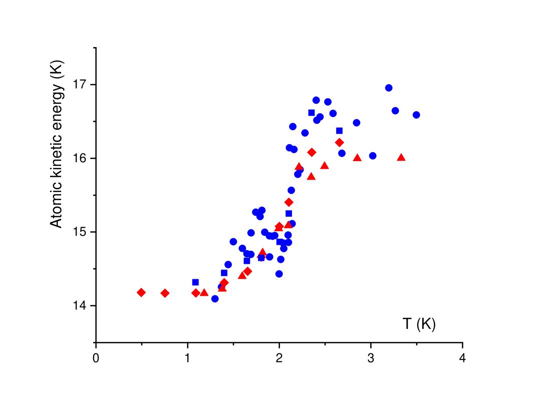
Figure 2: Atomic kinetic energy measured in different sets of neutron scattering experiments in liquid ⁴He (circles) and calculated in path integral Monte Carlo simulations (triangles) at atmospheric pressure ($T_{\lambda}=2.17$ K) Mayers et al. (2000). Squares correspond to more recent neutron experiments and diamonds to quantum Monte Carlo similations Prisk et al. (2017). Experimental uncertainties of energy are about 0.2-0.6 K.

Previously, the drop of $K$ at $T_{\lambda}$ was rationalised by assuming that a fraction of particles undergo BEC at $p=0$ and the rest having the energy in the uncondensed state Mayers et al. (1997, 2000); Prisk et al. (2017). Previous work did not explain the value of $K$ of 14 K below the jump at $T_{\lambda}$. This value readily comes out in the picture proposed here and from Eq. (3).

The experimental fluctuations of $K$ in Figure 2 are about $0.3$ K around 1 K Prisk et al. (2017). Using $E_{t}$ in (3), this corresponds to fluctuations of the relative energy and momentum of about 1-2%.

Below $T_{\lambda}$, the energy in Figure 2 may have contributions from $E_{t}$ and the average kinetic energy $\left<K_{g}\right>$ in the ground state which are close to each other as discussed in the previous section. In the range $\Delta T=2.5$-3.5 K above $T_{\lambda}$, $K$ in Figure 2 is larger than $E_{t}=14$ K at low temperature by approximately the amount of the thermal energy corresponding to $\Delta T$: $K=E_{t}+\Delta T$.

The second prediction concerns the dynamic structure factor $S({\bf q},\omega)$. The BECFE operates in a weakly-interacting gas of transits embedded in a quasi-rigid network of oscillating atoms (see Fig. 1c). The accumulation of transits in the state (3) should result in an increasing sharp peak of $S({\bf q},\omega)$ at frequency $\omega_{p}$ corresponding to the excitation energy, as $S({\bf q},\omega)\propto\delta(\omega-\omega_{p})$ Pines and Nozieres (1999). Excitations in a weakly-interacting Bose system are given by quasiparticles with the Hamiltonian

$$\begin{split}&H=E_{0}+\sum_{p\neq 0}\epsilon_{p}b_{p}^{+}b_{p}\\ &\epsilon_{p}=\sqrt{u_{s}^{2}p^{2}+\left(\frac{p^{2}}{2m}\right)^{2}}\end{split}$$ (8)

where $b_{p}^{+}$ and $b_{p}$ are creation and annihilation operators of elementary excitations with energy $\epsilon_{p}$, $u_{s}$ is the speed of sound in the system and where $\epsilon_{p}$ correspond to single-particle excitations $\epsilon_{p}=\frac{p^{2}}{2m}$ at large $p$ Landau and Lifshitz (1970); Pines and Nozieres (1999). The accumulation of transits in the state $E=E_{t}$ should then result in a sharp peak of $S({\bf q},\omega)$ below $T_{\lambda}$ at $\nu\approx 0.3$ THz as Eq. (3) predicts.

This prediction is supported by neutron scattering experiments Griffin (1993); Glyde (2018); Andersen et al. (1994); Talbot et al. (1988). Figures 3a,b show broad frequency distribution above $T_{\lambda}$ and a remarkable increase and sharpening of the peak below $T_{\lambda}$ (in some neutron scattering experiments, the width of the low-temperature peak can not be resolved Glyde (2018)). This is reminiscent of the sharp peak appearing in gases undergoing BEC at $p=0$. The peak is close to 0.3 THz as Eq. (3) predicts. The peak frequency can reduce at larger $q$ in the maxon-roton region where energy decreases with $q$ Glyde (2018).

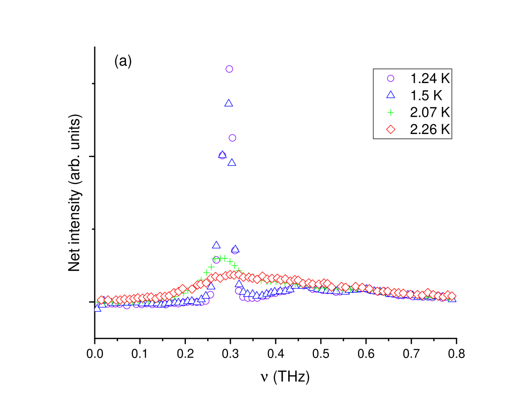
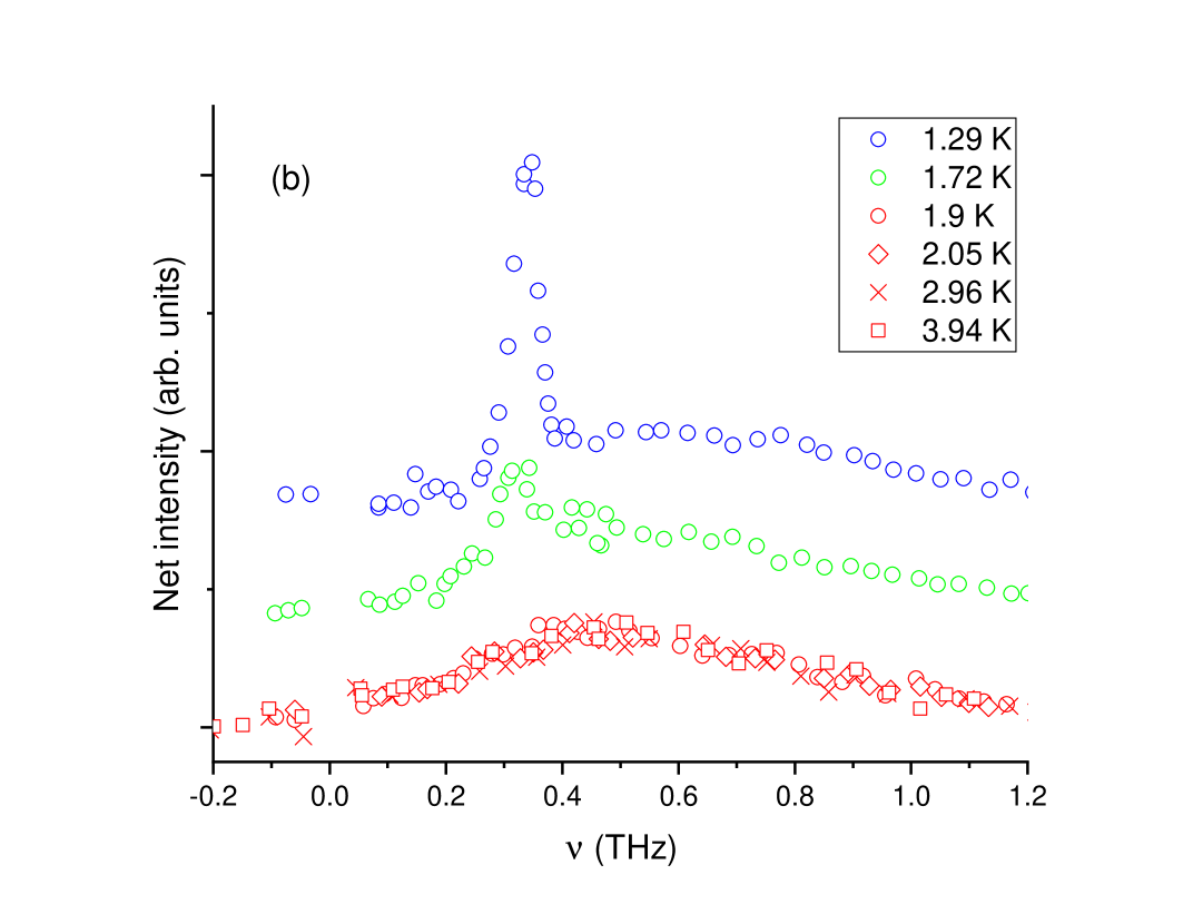
Figure 3: (a) $S(q,\omega)$ measured in neutron scattering experiments at atmospheric pressure at $q=1$ Å^-1. (b) $S(q,\omega)$ at 20 atm ($T_{\lambda}=1.928$ K) at $q=1.13$ Å^-1. The data are from Refs. Griffin (1993); Talbot et al. (1988).

As mentioned earlier, the sharp peak is predicted to take place at $q$ corresponding to single-particle excitations of transits. A detailed analysis attributes single-particle excitations to the maxon-roton part of the spectrum where $q$ is about 1 Å^-1 and larger Griffin (1993). Experimentally, sharp peaks are seen to develop for large $q$ in this range as seen in Figure 3 but not at smaller $q$. For example, no sharp change is seen in the scattering intensity below and above $T_{\lambda}$ at $q=0.4~{}$Å^-1 attributed to the phonon part of the spectrum Griffin (1993). This is consistent with our picture of transits in the BECFE state predicting peaks at large $q$. We note that at $q$ significantly exceeding those shown in Figure 3, the single-particle resonance no longer appears as a distinct peak due to experimental issues and other factors Griffin (1993).

Previously, the sharp resonance-type peaks in Fig. 3a,b were related to the BEC at $p=0$ which hybridizes single-particle excitations with collective density fluctuations Griffin (1993); Glyde (2018). It was later noted that the evidence for the BEC at $p=0$ is inconclusive because (a) the experimental data analysis giving the number of atoms in the state $p=0$, $n_{0}$, requires the prior knowledge of a physical model and (b) the data can be fit by models where $n_{0}=0$ (see, e.g., p. 175 of Ref. Prisk et al. (2017) and accompanying discussion and references). Previous interpretations involved parameters fitted to experimental data and did not physically explain why the resonance takes place at about 0.3 THz. This value readily comes out in the picture proposed here and from Eq. (3) in particular.

2.3 Discussion

The transit subsystem is related to the liquid flow as discussed earlier. Its wavefunction $\Psi_{T}$ can be written by approximating the transit motion by plane waves as mentioned earlier. In a model example where the transit speed is given by $c$ and where the fluctuations of transit speeds are not considered, the space variation of $\Psi_{T}$ is

$$\Psi_{T}=\prod\limits_{i=1}^{N_{t}}\exp\left(i\frac{mc}{\hbar}r_{i}\right)$$ (9)

where the single-particle functions are assumed normalised, $N_{t}$ is the number of transits in the BECFE state $p=p_{t}=mc$, $c=|{\bf c}_{i}|$ in Eq. (3), ${\bf c}_{i}$ is the transit velocity, $r_{i}=|{\bf r}_{i}(x,y,z)|$ ($0<r_{i}<a$) and ${\bf r}_{i}$ is the vector along the translational transit motion beginning at the transit starting point and defining the field of transit displacements in Figure 1c.

Although the product of plane waves in $\Psi_{T}$ may resemble the ideal gas, $\Psi_{T}$ describes a very different system: the gas of transits embedded in a quasi-rigid network of oscillating atoms in the liquid (this network is quasi-equilibrium and changes with relaxation time $\tau$ as discussed earlier). For this reason, the BECFE state does not suffer from the instability of the superfluid phase in the Bose gas related to the parabolic dispersion law and zero compressibility Pines and Nozieres (1999): the overall system is the liquid with a finite compressibility and speed of sound $c$ where the BECFE operates in a subsystem of transits.

Another important difference to BEC in gases is that the BECFE in the transit subsystem does not correspond to a fixed set of atoms and is dynamical. The probability of an atom to be in the transit state is $\frac{\tau_{\rm D}}{\tau}$, where $\tau_{\rm D}$ is the time this atom spends in the transit state and $\tau$ is the time between transits. In statistical equilibrium, the number of transits at each moment of time is therefore

$$N_{t}=N\frac{\tau_{\rm D}}{\tau}$$ (10)

where $N$ is the total number of atoms (by way of example, the ratio of viscosity at 1 K to the minimal viscosity in helium is about 2 Brewer and Edwards (1959), implying $\frac{\tau_{\rm D}}{\tau}$ of about one half). Hence the BECFE corresponds to a fixed set of $N_{t}$ transits during time $\tau_{\rm D}$ only, as illustrated in Figure 1c. In the next time period $\tau_{\rm D}$, a different set of transits is formed. After time $\tau$, all atoms participate in the transit motion and the BECFE. The liquid behavior and the superfluid response therefore correspond to a continuous time sequence of different transit subsets. The BECFE operates in each subset and is described by $\Psi_{T}$ in (9).

This dynamical picture addresses the long-standing problem of identifying a particular set of helium atoms with the superfluid and with the BEC state Landau and Lifshitz (1970); Landau (1941); Pines and Nozieres (1999); Pitaevskii and Stringari (2016): all atoms participate in the superfluid response and BECFE state but they do so at different times.

In earlier discussions, the BEC component is not identified with the superfluid component in the phenomenological two-fluid model describing the motion of thermal excitations Pitaevskii and Stringari (2016); Pines and Nozieres (1999). Similarly, we do not identify transits in the BECFE state with the superfluid component in the two-fluid model.

A macroscopically-occupied condensate state is related to superfluidity since modifying this state involves a simultaneous action on a large number of transits in the symmetrised macroscopic wavefunction Pines and Nozieres (1999). The spatially-varying condensate velocity, or the superfluid velocity, is ${\bf v}_{s}=\frac{\hbar}{m}\nabla S$, where $S$ is the phase of the condensate wavefunction $\psi_{c}$ Pines and Nozieres (1999). From Eq. (9), $\psi_{c}=\exp\left(i\frac{mc}{\hbar}r\right)$. This gives ${\bf v}_{s}=c\frac{{\bf r}}{r}={\bf c}_{i}$, whereas the net ${\bf v}_{s}$ is 0 because transits move in different directions. If the liquid moves with velocity ${\bf u}$, $\Psi_{T}$ in Eq. (9) becomes

$$\Psi_{T}=\prod\limits_{i=1}^{N_{t}}\exp\left(i\frac{m}{\hbar}({\bf c_{i}}+{\bf u}){\bf r}_{i}\right)$$ (11)

This gives ${\bf v}_{s}={\bf c}_{i}+{\bf u}$ and the net velocity of dissipationless flow of each transit subset ${\bf v}_{s}={\bf u}$. Experimentally, $v_{s}$ is limited by vortices Pines and Nozieres (1999); Pitaevskii and Stringari (2016). If ${\bf u}=-{\bf c_{i}}$ and an atom is stationary, the single-transit wavefunction becomes a constant and is removed from the BECFE. This makes an interesting connection to the macroscopic Landau criterion for the critical velocity set by $c$ Landau and Lifshitz (1970); Pines and Nozieres (1999).

We make three remarks related to how the proposed picture is related to previous work. First, the transits do not contribute to the liquid specific heat or other derivatives of thermodynamic potentials because $\exp(-E_{t}/T)$ in the partition function and its derivatives are negligibly small around 1 K. If Bose distribution $n_{p}$ were applicable to liquid helium, the weight of transits in $n_{p}$ would be close to zero. Recall that transits are athermal and that the transit energy comes from the zero-point oscillatory motion in a quasi-equilibrium cage: as the cage opens up, the oscillating atom becomes the transit undergoing a translational motion between two neighbouring positions (see discussion after Eq. (3)). Low-temperature thermodynamic properties of liquid helium are instead related to low-frequency phonons. This gives the specific heat $c_{v}\propto T^{3}$ Landau (1941), in agreement with experiments Greywall (1982). The anomaly of $c_{v}$ at $T_{\lambda}$ is interpreted as being due to the increasing size of permutation polygons corresponding to atomic exchanges Feynman (1953) (this picture does not consider BEC at $p=0$), consistent with path-integral Monte Carlo (PIMC) simulations Ceperley (1995). These permutations are enabled by mobile transits discussed here.

Second, the proposed picture addresses the issue related to BEC in the $p=0$ state in liquid helium raised early by Landau: the exchange of momentum between the immobile atoms in the state $p=0$ and excited mobile ones would result in friction, precluding superfluidity Landau (1941). This is not an issue in our picture where transits accumulate in their natural mobile states.

Third, earlier discussion of BEC in liquid helium at $p=0$ was seemingly based on the analogy with gases Pines and Nozieres (1999); Griffin (1993); Ceperley (1995); Pitaevskii and Stringari (2016); Annett (207); Leggett (2008); Glyde (2018). The data involved in this discussion are not inconsistent with the BECFE considered here. Theoretically, BEC in liquid helium at $p=0$ was discussed by generalising the criterion for the Bose gas and based on a large density matrix eigenvalue related to a large number of atoms in a particular state Penrose and Onsager (1956). This applies to BEC at any $p$ Pines and Nozieres (1999). Experimentally, ascertaining BEC at $p=0$ involves decomposing the measured momentum distribution into $n_{0}\delta(p)$ ($n_{0}$ is the number of atoms with $p=0$) and the rest, i.e. by assuming BEC at $p=0$ to begin with Prisk et al. (2017); Griffin (1993); Pitaevskii and Stringari (2016). The analysis of experimental data is model-dependent and involves problems in inverting scattering data to obtain a non-ambiguous momentum distribution. As a result, several models are consistent with $n_{0}=0$ (see, e.g., p. 175 of Ref. Prisk et al. (2017) and accompanying discussion). By similarly assuming BEC at $p=0$, the condensate fraction was calculated in PIMC simulations Ceperley (1995). It would be interesting to use these as well as dynamical simulations to quantify the BECFE state at $E=E_{t}$ related to transits. This would require larger systems with many transits.

We have not discussed the nature of the transition at $T_{\lambda}$ itself, leaving it for future work. A useful insight comes from the dynamical crossover at the Frenkel line marking the transition of particle motion from combined oscillatory and diffusive at low temperature below the line to purely diffusive above the line Cockrell et al. (2021); Proctor (2021); Cockrell and Trachenko (2022). If the low-temperature regime below $T_{\lambda}$ corresponds to combined oscillatory-diffusive particle motion, $E_{t}=$14 K in Figure 2 is related to the accumulation of transits in state (3). As noted in Section 2.1, this involves energy transfer between the zero-point energy and the energy of flowing transits in the BECFE state. This zero-point energy is due to the presence of the in-cage oscillatory component. This component disappears at higher temperature where particle dynamics becomes purely diffusive.

3 Summary

In summary, we discussed details of microscopic dynamics in liquids and explored its implications in liquid helium. This gives a way to discuss BEC in liquid helium which is consistent with microscopic liquid dynamics. In this picture, high mobility of liquid atoms results in the accumulation of transits in a finite-energy state. This is consistent with the experimentally measured kinetic energy of helium atoms below $T_{\lambda}$ and sharp peaks of scattered intensity at energy predicted by Eq. (3). More work is clearly needed to discuss the wealth of effects in liquid helium in this picture, including details of transition at $T_{\lambda}$.

I am grateful to A. E. Phillips and J. C. Phillips for discussions and EPSRC for support.

Appendix

Below is an example of a quantum-mechanical model of oscillatory-transit dynamics with continuous solutions in space and time. Other examples can be found too involving model modifications.

Let us consider how the wave function of the atom undergoing the transit changes from one oscillatory state to the next as shown in Figure 1a. We choose the $x$-direction along the transit motion. The wave function $f$ of the oscillating atom around $\sim 1$ K can be written as the oscillator wavefunction in the ground state because $\hbar\omega$, where $\omega$ is oscillation frequency, is about 54 K as calculated from the interatomic helium potential Annett (207): $f\propto\exp(-\alpha x^{2})$, where $\alpha=\frac{m\omega}{2\hbar}$ and $m$ is the mass of helium atom. The wavefunction of the transit $\psi(x)$ can be approximated by the plane wave as discussed in the main text. If $f_{1}(x)$ and $f_{2}(x)$ are the ground-state oscillatory wavefunctions before and after the transit, we can try the following wavefunctions describing the atom before, during and after the transit:

$$\begin{split}&f_{1}(x)=A\exp(-\alpha x^{2})\\ &\psi(x)=B\sin(kx-\phi)\\ &f_{2}(x)=C\exp(-\alpha(x-a)^{2})\end{split}$$ (12)

Let $\delta$ be the distance at which the particle leaves the first oscillatory state and becomes the transit as shown in Figure 1b and $a-\delta$ the distance at which the transit settles in the second oscillatory state, where $a$ is the interatomic separation and $\delta<\frac{a}{2}$. The continuity of the wavefunctions in (12) is ensured by equating $f_{1}(x)$ and $\psi(x)$ and their derivatives at $x=\delta$ and equating $\psi(x)$ and $f_{2}(x)$ and their derivatives at $x=a-\delta$. This gives

$$\begin{split}&A\exp(-\alpha\delta^{2})=B\sin(k\delta-\phi)\\ &-2A\alpha\delta\exp(-\alpha\delta^{2})=Bk\cos(k\delta-\phi)\\ &C\exp(-\alpha\delta^{2})=B\sin(k(a-\delta))-\phi)\\ &2C\alpha\delta\exp(-\alpha\delta^{2})=Bk\cos(k(a-\delta)-\phi)\end{split}$$ (13)

The first and second pair of equations have non-trivial solutions each if

$$\begin{split}&-2\alpha\delta=\frac{k\cos(k\delta-\phi)}{\sin(k\delta-\phi)}\\ &2\alpha\delta=\frac{k\cos(k(a-\delta)-\phi)}{\sin(k(a-\delta)-\phi)}\end{split}$$ (14)

The two equations (14) are compatible if $\tan(k\delta-\phi)=-\tan(k(a-\delta)-\phi)$, giving, bar the periodic argument $\pm\frac{\pi n}{2}$, $\phi=\frac{ka}{2}$. Using this $\phi$ in (14) gives

$$\begin{split}&\tan y=\chi y\\ &y=k\left(\frac{a}{2}-\delta\right)\\ &\chi=\frac{1}{2\alpha\delta\left(\frac{a}{2}-\delta\right)}=\frac{a^{2}}{\delta\left(\frac{a}{2}-\delta\right)}\end{split}$$ (15)

In the last equality, we recalled $\alpha=\frac{m\omega}{\hbar}$ and used the uncertainty relation for the transit localised within distance $a$ in Eq. (4), resulting in $\alpha=\frac{1}{a^{2}}$.

The equation for $y$ has a solution in the first half-period of $\tan y$ because $\chi>1$ in the considered range $0<\delta<\frac{a}{2}$.

In addition to the continuity of the wavefunctions in space, this model also ensures their time continuity. The time dependence of the three wavefunctions is

$$\begin{split}&f_{1}(x,t)\propto f_{1}(x)\exp\left(-\frac{iE_{g}t}{\hbar}\right)\\ &\psi(x)\propto\phi_{1}(x)\exp\left(-\frac{iE_{t}t}{\hbar}\right)\\ &f_{2}(x,t)\propto f_{2}(x)\exp\left(-\frac{iE_{g}t}{\hbar}\right)\end{split}$$ (16)

where $E_{g}=\frac{\hbar\omega}{2}$ is the oscillatory ground state energy and $E_{t}=\frac{p^{2}}{2m}$ is the transit kinetic energy.

Setting $v=a\omega$ as earlier, $E_{g}$ and $E_{t}$ become equal: $E_{t}=\frac{m\omega^{2}a^{2}}{2}$ becomes $E_{g}=\frac{\hbar\omega}{2}$ once the uncertainty relation (4) is used, implying the time continuity of the wavefunctions in the oscillatory-transit states.

References

- Landau and Lifshitz (1970) L. D. Landau and E. M. Lifshitz, Statistical Physics, part 1. (Pergamon Press, 1970).
- Pitaevskii (1994) L. P. Pitaevskii, Physical Encyclopedia, ed. by A. M. Prokhorov 4, 670 (1994).
- Kirkwood (1968) J. G. Kirkwood, Theory of liquids (Gordon and Breach, 1968).
- Born and Green (1946) M. Born and H. S. Green, Proc. Royal Soc. London 19, 188 (1946).
- Zwanzig (1954) R. Zwanzig, J. Chem. Phys. 22, 1420 (1954).
- Barker and Henderson (1976) J. A. Barker and D. Henderson, Rev. Mod. Phys. 48, 587 (1976).
- Egelstaff (1994) P. A. Egelstaff, An Introduction to the Liquid State (Oxford University Press, 1994).
- Faber (1972) T. E. Faber, An Introduction fo the Theory of Liquid Metals (Cambridge University Press, 1972).
- March (1990) N. H. March, Liquid Metals, Concepts and Theory (Cambridge University Press, 1990).
- March and Tosi (1991) N. H. March and M. P. Tosi, Atomic Dynamics in Liquids (Dover Publications, 1991).
- Tabor (1993) D. Tabor, Gases, liquids and solids (Cambridge University Press, 1993).
- Balucani and Zoppi (2003) U. Balucani and M. Zoppi, Dynamics of the Liquid State (Oxford University Press, 2003).
- Barrat and Hansen (2003) J. L. Barrat and J. P. Hansen, Basic Concepts for Simple and Complex Liquids (Cambridge University Press, 2003).
- Hansen and McDonald (2013) J. P. Hansen and I. R. McDonald, Theory of Simple Liquids (Elsevier, 2013).
- Trachenko and Brazhkin (2016) K. Trachenko and V. V. Brazhkin, Rep. Prog. Phys. 79, 016502 (2016).
- Wallace (1998) D. C. Wallace, Phys. Rev. E 57, 1717 (1998).
- Wallace (2002) D. C. Wallace, Statistical physics of crystals and liquids (World Scientific, 2002).
- Proctor (2020) J. Proctor, Phys. Fluids 32, 107105 (2020).
- Proctor (2021) J. Proctor, The liquid and supercritical states of matter (CRC Press, 2021).
- Chen (2022) G. Chen, Journal of Heat Transfer 144, 010801 (2022).
- Ziman (1979) J. M. Ziman, Models of Disorder (Cambridge University Press, 1979).
- Parisi and Zamponi (2010) G. Parisi and F. Zamponi, Rev. Mod. Phys. 82, 789 (2010).
- Weeks et al. (1971) J. D. Weeks, D. Chandler, and H. C. Andersen, J. Chem. Phys. 54, 5237 (1971).
- Chandler et al. (1983) D. Chandler, J. D. Weeks, and H. C. Andersen, Science 220, 788 (1983).
- Rosenfeld and Tarazona (1998) Y. Rosenfeld and P. Tarazona, Molecular Physics 95, 141 (1998).
- Frenkel (1947) J. Frenkel, Kinetic Theory of Liquids (Oxford University Press, 1947).
- Bardeen et al. (1957) J. Bardeen, L. N. Cooper, and J. R. Schrieffer, Phys. Rev. 108, 1175 (1957).
- Pines and Nozieres (1999) D. Pines and P. Nozieres, Theory Of Quantum Liquids (Westview Press, 1999).
- Griffin (1993) A. Griffin, Excitations in a Bose-condensed liquid (Cambridge Univesity Press, 1993).
- Ceperley (1995) D. M. Ceperley, Rev. Mod. Phys. 67, 279 (1995).
- Nakayama and Makri (2005) A. Nakayama and N. Makri, PNAS 102, 4230 (2005).
- Cockrell et al. (2021) C. Cockrell, V. V. Brazhkin, and K. Trachenko, Physics Reports 941, 1 (2021).
- Wallace et al. (2001) D. C. Wallace, E. D. Chisolm, and B. E. Clements, Phys. Rev. E 64, 011205 (2001).
- Dyre (2006) J. C. Dyre, Rev. Mod. Phys. 78, 953 (2006).
- Pitaevskii and Stringari (2016) L. Pitaevskii and S. Stringari, Bose-Einstein Condensation and Superfluidity (Oxford University Press, 2016).
- Annett (207) J. F. Annett, Superconductivity, Superfluids and Condensates (Oxford University Press, 207).
- Leggett (2008) A. J. Leggett, Quantum Liquids (Oxford University Press, 2008).
- Glyde (2018) H. R. Glyde, Rep. Prog. Phys. 81, 014501 (2018).
- Balibar (2017) S. Balibar, C. R. Physique 18, 586 (2017).
- Prisk et al. (2017) T. R. Prisk, M. S. Bryan, P. E. Sokol, G. E. Granroth, S. Moroni, and Boninsegni, J. Low Temp. Phys. 189, 158 (2017).
- Landau (1941) L. Landau, J. Phys. USSR 5, 71 (1941).
- Trachenko and Brazhkin (2020) K. Trachenko and V. V. Brazhkin, Sci. Adv. 6, aba3747 (2020).
- Trachenko et al. (2020) K. Trachenko, B. Monserrat, C. J. Pickard, and V. V. Brazhkin, Sci. Adv. 6, eabc8662 (2020).
- Yukalov (1980) V. I. Yukalov, Physica A 100, 431 (1980).
- Liberto et al. (2011) M. D. Liberto, O. Tieleman, V. Branchina, and C. M. Smith, Phys. Rev. A 84, 013607 (2011).
- Hick et al. (2010) J. Hick, F. Sauli, A. Kreisel, and P. Kopietz, Eur. Phys. J. B 78, 429 (2010).
- Mayers et al. (1997) J. Mayers, C. Andreani, and D. Colognesi, J. Phys.: Condens. Matt. 9, 10639 (1997).
- Mayers et al. (2000) J. Mayers, Albergamo, and D. Timmis, Physica B 276-278, 811 (2000).
- Andersen et al. (1994) K. H. Andersen, W. G. Stirling, R. Scherm, A. Stunault, B. Fåk, H. Godfrin, and A. J. Dianoux, J. Phys.: Condens. Matt. 6, 821 (1994).
- Talbot et al. (1988) E. F. Talbot, H. R. Glyde, W. G. Stirling, and E. C. Svensson, Phys. Rev. B 38, 11229 (1988).
- Brewer and Edwards (1959) D. F. Brewer and D. O. Edwards, Proc. R. Soc. London A 251, 247 (1959).
- Greywall (1982) D. S. Greywall, Phys. Rev. B 18, 2127 (1982).
- Feynman (1953) R. Feynman, Phys. Rev. 90, 1116 (1953).
- Penrose and Onsager (1956) O. Penrose and L. Onsager, Phys. Rev. 104, 576 (1956).
- Cockrell and Trachenko (2022) C. Cockrell and K. Trachenko, Sci. Adv. 8, eabq5183 (2022).