Symbolic Runtime Verification for Monitoring under Uncertainties and Assumptions

Abstract

Runtime Verification deals with the question of whether a run of a system adheres to its specification. This paper studies runtime verification in the presence of partial knowledge about the observed run, particularly where input values may not be precise or may not be observed at all. We also allow declaring assumptions on the execution which permits to obtain more precise verdicts also under imprecise inputs. To this end, we show how to understand a given correctness property as a symbolic formula and explain that monitoring boils down to solving this formula iteratively, whenever more and more observations of the run are given. We base our framework on stream runtime verification, which allows to express temporal correctness properties not only in the Boolean but also in richer logical theories. While in general our approach requires to consider larger and larger sets of formulas, we identify domains (including Booleans and Linear Algebra) for which pruning strategies exist, which allows to monitor with constant memory (i.e. independent of the length of the observation) while preserving the same inference power as the monitor that remembers all observations. We empirically exhibit the power of our technique using a prototype implementation under two important cases studies: software for testing car emissions and heart-rate monitoring.

1 Introduction

In this paper we study runtime verification (RV) for imprecise and erroneous inputs, and describe a solution—called symbolic monitoring—that can exploit assumptions about the input and the system under analysis. Runtime verification is a dynamic verification technique in which a given run of a system is checked against a specification, typically a correctness property (see [13, 22, 1]). In online monitoring a monitor is synthesized from the given correctness property, which attempts to produce a verdict incrementally from the input trace. Originally, variants of LTL [25] tailored to finite runs have been employed in RV to formulate properties (see [3] for a comparison on such logics). However, since RV requires to solve a variation of the word problem and not the harder model-checking problem, richer logics than LTL have been proposed that allow richer data and verdicts [10, 14]. Lola [9] proposes stream runtime verification (SRV) where monitors are described declaratively and compute output streams of verdicts from inputs streams (see also [20, 12]). The development of this paper is based on Lola.

(a) A Specification	(b) Monitor run with perfect information
(c) Interval abstraction	(d) Symbolic Monitor

Figure 1: An example specification (a) and three monitors: (b) with perfect observability, (c) with an interval abstract domain, (d) a symbolic monitor developed in this paper. The symbolic monitor is enriched with the additional constraint that $1\leq\textrm{{ld}}^{0}\leq 5$.

Example 1

Fig. 1(a) shows a Lola specification with ld as input stream (the load of a CPU), acc as an output stream that represents the accumulated load, computed by adding the current value of ld and subtracting the third last value. Finally, ok checks whether acc is below $15$. The expression $\textrm{{acc}}[-1|0]$ denotes the value of acc in the previous time point and $0$ as default value if no previous time point exists.

Such a specification allows a direct evaluation strategy whenever values on the input streams arrive. If, for example, $\textrm{{ld}}=3$ in the first instant, acc and ok evaluate to $3$ and tt, respectively. Reading subsequently $4,5,7$ results in $7,12,16$ for acc and a violation is identified on stream ok. This is shown in Fig. 1(b).

A common obstacle in runtime verification is that in practice sometimes input values are not available or not given precisely, due to errors in the underlying logging functionality or technical limitations of sensors. In Fig. 1(c) the first value on ld is not obtained (but we assume that all values of ld are between $1$ and $5$). One approach is to use interval arithmetic, which can be easily encoded as a rich domain in Lola, and continue the computation when obtaining $4$, $5$ and $7$. However, at time $4$ the monitor cannot know for sure whether ok has been violated, as the interval $[12,20]$ contains $15$. This approach based on abstract interpretation [8] was pursued in [21] and suffers from this limitation. If the unknown input on ld is denoted symbolically by $\textrm{{ld}}^{0}$ we still deduce that ok holds at time points $1$ to $3$. For time point $4$, however, the symbolic representation $\textrm{{acc}}^{4}=\textrm{{acc}}^{3}+7-\textrm{{ld}}^{0}=\textrm{{ld}}^{0}+9+7-\textrm{{ld}}^{0}=16$ allows to infer that ok is clearly violated! This is shown in Fig. 1(d).∎

Example 1 illustrates the first insight pursued in this paper: that Symbolic monitoring is more precise than monitoring using abstract domains.

Clearly, an infinite symbolic unfolding of a specification and all the assumptions with subsequent deduction is practically infeasible. Therefore, we perform online monitoring unfolding the specification as time increases. We show that a monitor based on deducing verdicts using this partial symbolic unfolding is both sound and perfect in the sense that the monitor only produces correct verdicts and these are as precise verdicts as possible with the information provided. Symbolic monitoring done in this straightforward way, however, comes at a price: the unfolded specification grows as more unknowns and their inter-dependencies become part of the symbolic unfolding. For example, in the run in Fig. 1(d) as more unknown ld values are received, more variables $\textrm{{ld}}^{i}$ will be introduced, which may make the size of the symbolic formula dependent on the trace length. We show that for certain logical theories, the current verdict may be still be computed even after summarizing the history into a compact symbolic representation, whose size is independent of the trace length. For other theories, preserving the full precision of symbolic monitoring requires an amount of memory that can grow with the trace length. More precisely, we show that for the theories of Booleans and of Linear Algebra, bounded symbolic monitors exist while this is not the case for the combined theory, which is the second insight presented in this paper.

We have evaluated our approach on two realistic cases studies, the Legal Driving Cycle [18, 5] and an ECG heartbeat analysis (following the Lola implementation in [11], see also [24, 26]) which empirically validate our symbolic monitoring approach, including constant monitoring on long traces. When intervals are given for unknown values, our method provides precise answers more often than previous approaches based on interval domains [21]. Especially in the ECG example, these methods are unable to recover once the input is unknown for even a short time, but our symbolic monitors recover and provide again precise results, even when the input was unknown for a larger period.

Related Work.

Monitoring LTL for traces with mutations (errors) is studied in [16] where properties are classified according to whether monitors can be built that are resilient against the mutation. However, [16] only considers Boolean verdicts and does not consider assumptions. The work in [21] uses abstract interpretation to soundly approximate the possible verdict values when inputs contain errors for the SRV language TeSSLa [7].

Calculating and approximating the values that programs compute is central to static analysis and program verification. Two traditional approaches are symbolic execution [17] and abstract interpretation [8] which frequently require over-approximations to handle loops. In monitoring, a step typically does not contain loops, but the set of input variables (unlike in program analysis) grows. Also, a main concern of RV is to investigate monitoring algorithms that are guaranteed to execute with constant resources. Works that incorporate assumptions when monitoring include [15, 6, 19] but uncertainty is not considered in these works, and verdicts are typically Boolean. Note that bounded model checking [4] also considers bounded unfoldings, but it does not solve the problem of building monitors of constant memory for successive iterations.

In summary, our contributions are: (1) A symbolic monitoring algorithm that dynamically unfolds the specification, collects precise and imprecise input readings, and instantiates assumptions generating a conjunction of formulas. This representation can be used to deduce verdicts even under uncertainty, to precisely recover automatically for example under windows of uncertainty, and even to anticipate verdicts. (2) A pruning method for certain theories (Booleans and Linear Algebra) that guarantees bounded monitoring preserving the power to compute verdicts. (3) A prototype implementation and empirical evaluation on realistic case studies.

All missing proofs appear in the appendix.

2 Preliminaries

We use Lola [9] to express our monitors. Lola uses first-order sorted theories to build expressions. These theories are interpreted in the sense that every symbol is a both constructor to build expressions, and an evaluation function that produces values from the domain of results from values from the domains of the arguments. All sorts of all theories that we consider include the $=$ predicate.

A synchronous stream $s$ over a non-empty data domain $\mathbb{D}$ is a function $s:\mathcal{S}_{\mathbb{D}}:=\mathbb{T}\to\mathbb{D}$ assigning a value of $\mathbb{D}$ to every element of $\mathbb{T}$ (timestamp). We consider infinite streams ($\mathbb{T}=\mathbb{N}$) or finite streams with a maximal timestamp $t_{\textrm{max}}$ ($\mathbb{T}=[0\ldots{}t_{\textrm{max}}]$). For readability we denote streams as sequences, so $s=\langle 1,2,4\rangle$ stands for $s:\{1,2,3\}\rightarrow\mathbb{N}$ with $s(0)=1,s(1)=2,s(2)=4$. A Lola specification describes a transformation from a set of input streams to a set of output streams.

Syntax.

A Lola specification $\varphi=(I,O,E)$ consists of a set $I$ of typed variables that denote the input streams, a set $O$ of typed variables that denote the output steams, and $E$ which assigns to every output stream variable $y\in O$ a defining expression $E_{y}$. The set of expressions over $I\cup O$ of type $\mathbb{D}$ is denoted by $E_{\mathbb{D}}$ and is recursively defined as: $E_{\mathbb{D}}=c\mid s[o|c]\mid f(E_{\mathbb{D}_{1}},...,E_{\mathbb{D}_{n}})\mid ite(E_{\mathbb{B}},E_{\mathbb{D}},E_{\mathbb{D}})$, where $c$ is a constant of type $\mathbb{D}$, $s\in I\cup O$ is a stream variable of type $\mathbb{D}$, $o\in\mathbb{Z}$ is an offset and $f$ a total function $\mathbb{D}_{1}\times\dots\times\mathbb{D}_{n}\rightarrow\mathbb{D}$ (ite is a special function symbol to denote if-then-else). The intended meaning of the offset operator $s[o|c]$ is to represent the stream that has at time $t$ the value of stream $s$ at $t+o$, and value $c$ used if $t+o\notin\mathbb{T}$. A particular case is when the offset is $o=0$ in which case $c$ is not needed, which we shorten by $s[\textrm{{now}}]$. Function symbols allow to build terms that represent complex expressions. The intended meaning of the defining equation $E_{y}$ for output variable $y$ is to declaratively define the values of stream $y$ in terms of the values of other streams.

Semantics.

The semantics of a Lola specification $\varphi$ is a mapping from input to output streams. Given a tuple of concrete input streams ($\Sigma=(\sigma_{1},\dots,\sigma_{n})\in\mathcal{S}_{\mathbb{D}_{1}}\times\dots\times\mathcal{S}_{\mathbb{D}_{n}}$) corresponding to input stream identifier $s_{1},\dots,s_{n}$ and a specification $\varphi$ the semantics of an expression $\llbracket\cdot\rrbracket_{\Sigma,\varphi}:E_{\mathbb{D}}\rightarrow\mathcal{S}_{\mathbb{D}}$ is iteratively defined as:

• $\llbracket c\rrbracket_{\Sigma,\varphi}(t)=c$

• $\llbracket s[o|c]\rrbracket_{\Sigma,\varphi}(t)=\begin{cases}\sigma_{i}(t+o)&\textrm{if }t+o\in\mathbb{T}\textrm{ and }s=s_{i}\in I\textrm{ (input stream)}\\ \llbracket e\rrbracket_{\Sigma,\varphi}(t+o)&\textrm{if }t+o\in\mathbb{T}\textrm{ and }E_{s}=e\textrm{ (output stream)}\\ c&\textrm{otherwise}\end{cases}$

• $\llbracket f(e_{1},...,e_{n})\rrbracket_{\Sigma,\varphi}(t)=f(\llbracket e_{1}\rrbracket_{\Sigma,\varphi}(t),\ldots,\llbracket e_{n}\rrbracket_{\Sigma,\varphi}(t))$

• $\llbracket ite(e_{1},e_{2},e_{3})\rrbracket_{\Sigma,\varphi}(t)=\begin{cases}\llbracket e_{2}\rrbracket_{\Sigma,\varphi}(t)&\textrm{if }\llbracket e_{1}\rrbracket_{\Sigma,\varphi}(t)=\textrm{{tt}}\\ \llbracket e_{3}\rrbracket_{\Sigma,\varphi}(t)&\textrm{if }\llbracket e_{1}\rrbracket_{\Sigma,\varphi}(t)=\textrm{{ff}}\end{cases}$

The semantics of $\varphi$ is a map ($\llbracket\varphi\rrbracket:(\mathcal{S}_{\mathbb{D}_{1}}\times\dots\times\mathcal{S}_{\mathbb{D}_{n}})\rightarrow(\mathcal{S}_{\mathbb{D}^{\prime}_{1}}\times\dots\times\mathcal{S}_{\mathbb{D}^{\prime}_{m}}$) defined as $\llbracket\varphi\rrbracket(\sigma_{1},...,\sigma_{n})=(\llbracket e^{\prime}_{1}\rrbracket_{\Sigma,\varphi},\ldots,\llbracket e^{\prime}_{m}\rrbracket_{\Sigma,\varphi})$. The evaluation map $\llbracket\cdot\rrbracket_{\Sigma,\varphi}$ is well-defined if the recursive evaluation above has no cycles. This acyclicity can be easily checked statically (see [9]).

In online monitoring monitors receive the values incrementally. The very efficiently monitorable fragment of Lola consists of specifications where all offsets are negative or 0 (without transitive 0 cycles). It is well-known that the very efficiently monitorable specifications (under perfect information) can be monitored online in a trace length independent manner. In the rest of the paper we also assume that all Lola specifications come with $-1$ or $0$ offsets. Every specification can be translated into such a normal form by introducing additional streams (flattening).

In this paper we investigate online monitoring under uncertainty for three special fragments of Lola, depending on the data theories used:

• Propositional Logic ($\textrm{Lola}_{\mathbb{B}}$): The data domain of all streams is the Boolean domain $\mathbb{D}=\mathbb{B}=\{\textrm{{tt}},\textrm{{ff}}\}$ and available functions are $\land,\neg$.

• Linear Algebra ($\textrm{Lola}_{\mathcal{LA}}$): The data domain of all streams are real numbers $\mathbb{D}=\mathbb{R}$ and every stream definition has the form $c_{0}+c_{1}*s_{0}[o_{1}|d_{1}]+\dots+c_{n}*s_{n}[o_{n}|d_{n}]$ where $c_{i}$ are constants.

• Mixed ($\textrm{Lola}_{\mathbb{B}/\mathcal{LA}}$): The data domain is $\mathbb{B}$ or $\mathbb{R}$. Every stream definition is either contained in the Propositional Logic fragment extended by the functions $<,\leq,=$ or in the Linear Algebra fragment.

3 A Framework for Symbolic Monitoring

In this section we introduce a general framework for monitoring using symbolic computation, where the specification and the information collected by the monitor (including assumptions and precise and imprecise observations) are presented symbolically.

3.1 Symbolic Expressions

Consider a specification $\varphi=(I,O,E)$. We will use symbolic expressions to capture the relations between the different streams at different points in time. We introduce the instant variables $x^{t}$ for a given stream variable $x\in I\cup{}O$ and instant $t\in\mathbb{T}$. The type of $x^{t}$ is that of $x$. Considering Example 1, $\textrm{{ld}}^{3}$ represents the real value that corresponds to the input stream ld at instant $3$ which is $7$. The set of instant variables is $V=(I\cup O)\times\mathbb{T}$.

Definition 1 (Symbolic Expression)

Let $\varphi$ be a specification and $\mathcal{A}$ a set of variables that contains all instant variables (that is $V\subseteq\mathcal{A}$), the set of symbolic expressions $\overline{\mathbb{D}}$ is the smallest set containing (1) all constants $c$ and all symbols in $a\in\mathcal{A}$, (2) all expressions $f(t_{1},\ldots,t_{n})$ where $f$ is a constructor symbol of type $\mathbb{D}_{1}\times\dots\times\mathbb{D}_{n}\rightarrow\mathbb{D}$ and $t_{i}$ are elements of $\overline{\mathbb{D}}$ of type $\mathbb{D}_{i}$.

We use $\textit{Expr}^{\mathbb{D}}_{\varphi}(\mathcal{A})$ for the set of symbolic expressions of type $\mathbb{D}$ (and drop $\varphi$ and $\mathcal{A}$ when it is clear from the context).

Example 2

Consider again Example 1. The symbolic expression $\textrm{{acc}}^{3}+\textrm{{ld}}^{4}$, of type $\mathbb{R}$, represents the addition of the load at instant $4$ and the accumulator at instant $3$. Also, $\textrm{{acc}}^{4}=\textrm{{acc}}^{3}+\textrm{{ld}}^{4}$ is a predicate (that is, a $\mathbb{B}$ expression) that captures the value of acc at instant $4$. The symbolic expression $\textrm{{ld}}^{1}=4$ corresponds to the reading of the value $4$ for input stream ld at instant $1$. Finally, $1\leq\textrm{{ld}}^{0}\mathrel{\wedge}\textrm{{ld}}^{0}\leq 5$ corresponds to the assumption at time $0$ that ld has value between $1$ and $5$. ∎

3.2 Symbolic Monitor Semantics

We define the symbolic semantics of a Lola specification $\varphi=(I,O,E)$ as the expressions that result by instantiating the defining equations $E$.

Definition 2 (Symbolic Monitor Semantics)

The map $\llbracket\cdot\rrbracket_{\varphi}:E_{\mathbb{D}}\mathrel{\rightarrow}\mathbb{T}\mathrel{\rightarrow}\textit{Expr}^{\mathbb{D}}_{\varphi}$ is defined as $\llbracket c\rrbracket_{\varphi}(t)=c$ for constants, and

• $\llbracket f(e_{1},\ldots,e_{n})\rrbracket_{\varphi}(t)=f(\llbracket e_{1}\rrbracket_{\varphi}(t),\ldots,\llbracket e_{n}\rrbracket_{\varphi}(t))$

• $\llbracket s[o|c]\rrbracket_{\varphi}(t)=s^{t+o}$ if $t+o\in\mathbb{T}$, or $\llbracket s[o|c]\rrbracket_{\varphi}(t)=c$ otherwise.

The symbolic semantics of a specification $\varphi$ is the map $\llbracket\cdot\rrbracket_{\textit{sym}}:\mathbb{T}\mathrel{\rightarrow}2^{\textit{Expr}_{\varphi}^{\mathbb{B}}}$ defined as $\llbracket\varphi\rrbracket_{\textit{sym}}^{t}=\{y^{t}=\llbracket E_{y}\rrbracket_{\varphi}(t)\;|\;\text{ for every $y\in O$}\}.$

A slight modification of the symbolic semantics allows to obtain equations whose right hand sides only have input instant variables:

• $\llbracket s[o|c]\rrbracket_{\varphi}(t)=s^{t+o}$          if $t+o\in\mathbb{T}$ and $s\in I$

• $\llbracket s[o|c]\rrbracket_{\varphi}(t)=\llbracket e_{s}\rrbracket(t+o)$ if $t+o\in\mathbb{T}$ and $s\in O$

• $\llbracket s[o|c]\rrbracket_{\varphi}(t)=c$ otherwise

We call this semantics the symbolic unrolled semantics, which corresponds to what would be obtained by performing equational reasoning (by equational substitution) in the symbolic semantics.

Example 3

Consider again the specification $\varphi$ in Example 1. The first four elements of $\llbracket\varphi\rrbracket_{\textit{sym}}$ are (after simplifications like $0+x=x$ etc.):

$$\footnotesize\begin{array}[]{|c|c|c|c|}\hline\cr 0&1&2&3\\ \hline\cr\textrm{{acc}}^{0}=\textrm{{ld}}^{0}&\textrm{{acc}}^{1}=\textrm{{acc}}^{0}+\textrm{{ld}}^{1}&\textrm{{acc}}^{2}=\textrm{{acc}}^{1}+\textrm{{ld}}^{2}&\textrm{{acc}}^{3}=\textrm{{acc}}^{2}+\textrm{{ld}}^{3}-\textrm{{ld}}^{0}\\ \textrm{{ok}}^{0}=\textrm{{acc}}^{0}\leq 15&\textrm{{ok}}^{1}=\textrm{{acc}}^{1}\leq 15&\textrm{{ok}}^{2}=\textrm{{acc}}^{2}\leq 15&\textrm{{ok}}^{3}=\textrm{{acc}}^{3}\leq 15\\ \hline\cr\end{array}$$

Using the unrolled semantics the equations for ok would be, at time $0$, $\textrm{{ok}}^{0}=\textrm{{ld}}^{0}\leq 15$, and at time $1$, $\textrm{{ok}}^{1}=\textrm{{ld}}^{0}+\textrm{{ld}}^{1}\leq 15$. In the unrolled semantics all equations contain only instant variables that represent inputs.∎

Recall that the denotational semantics of Lola monitor specifications in Section 2 maps every tuple of input streams into a tuple of output streams, that is $\llbracket\varphi\rrbracket:\mathcal{S}_{\mathbb{D}_{1}}\times\dots\times\mathcal{S}_{\mathbb{D}_{n}}\mathrel{\rightarrow}\mathcal{S}_{\mathbb{D}^{\prime}_{1}}\times\dots\times\mathcal{S}_{\mathbb{D}^{\prime}_{m}}.$ The symbolic semantics also has a denotational meaning even without receiving the input stream, defined as follows.

Definition 3 (Denotational semantics)

Let $\varphi=(I,O,E)$ be a specification with $I=(x_{1},\ldots,x_{n})$ and $O=(y_{1},\ldots,y_{m})$. The denotational semantics of a set of equations $E\subseteq\textit{Expr}^{\mathbb{B}}_{\varphi}$ $\llbracket E\rrbracket_{\textit{den}}\subseteq\mathcal{S}_{\mathbb{D}_{1}}\times\dots\times\mathcal{S}_{\mathbb{D}_{n}}\times\mathcal{S}_{\mathbb{D}^{\prime}_{1}}\times\dots\times\mathcal{S}_{\mathbb{D}^{\prime}_{m}}$ is:

$$\llbracket E\rrbracket_{\textit{den}} =\{(\sigma_{1},\ldots,\sigma_{n},\sigma_{1}^{\prime},\ldots,\sigma^{\prime}_{m})\;|\;\text{ for every $e\in E$ }$$

$$\hskip 30.00005pt\{x_{1}^{t}=\sigma_{1}(t),\ldots,x_{n}^{t}=\sigma_{n}(t),y_{1}^{t}=\sigma^{\prime}_{1}(t),\ldots,y_{m}^{t}=\sigma^{\prime}_{m}(t)\}\models e\}$$

linecolor=cyan,backgroundcolor=cyan!25,bordercolor=cyan]ML@all: $t$ is always a finite value and for any $t$ it should work. If we have a continuous setting, we may say something regarding the fixpoint $t\to\infty$ but we don’t care here. In other words: Yes, we do not discuss that the semantics for $\infty$ is say tt but the monitor will always say ff. We do not support full anticipation. Cesar: Idea for future paper.

Using the previous definition, $\llbracket\bigcup_{i\leq t}\llbracket\varphi\rrbracket_{\textit{sym}}^{i}\rrbracket_{\textit{den}}$ corresponds to all the tuples of streams of inputs and outputs that satisfy the specification $\varphi$ up to time $t$.

3.2.1 A Symbolic Encoding of Inputs, Constraints and Assumptions.

Input readings can also be defined symbolically as follows. Given an instant $t$, an input stream variable $x$ and a value $v$, the expression $x^{t}=v$ captures the precise reading of $v$ at $t$ on $x$. Imprecise readings can also be encoded easily. For example, if at instant $3$ an input of value $7$ for ld is received by a noisy sensor (consider a $1$ unit of tolerance), then $6\leq\textrm{{ld}}^{3}\leq 8$ represents the imprecise reading.

Assumptions are relations between the variables that we assume to hold at all positions, which can be encoded as stream expressions of type $\mathbb{B}$. For example, the assumption that the load is always between $1$ and $10$ is $1\leq\textrm{{ld}}[\textrm{{now}}]\leq 10$. Another example, $\textrm{{ld}}[-1|0]+1\geq\textrm{{ld}}[\textrm{{now}}]$ which encodes that ld cannot increase more than $1$ per unit of time. We use $A$ for the set of assumptions associated with a Lola specification $\varphi$ (which are a set of stream expressions of type $\mathbb{B}$ over $I\cup O$).

3.3 A Symbolic Monitoring Algorithm

Based on the previous definitions we develop our symbolic monitoring algorithm shown in Alg. 1. Line 3 instantiates the new equations and assumptions from the specification for time $t$. Line 4 incorporates the readings (perfect or imperfect). Line 5 performs evaluations and simplifications, which is dependent on the particular theory. In the case of past-specifications with perfect information this step boils down to substitution and evaluation. Line $6$ produces the output of the monitor.

1

2$t\leftarrow 0$ and $E\leftarrow\emptyset$;

3 while $t\in\mathbb{T}$ do

4       $E\leftarrow E\cup\llbracket\varphi\rrbracket_{\textit{sym}}^{t}\cup\llbracket A^{t}\rrbracket_{\varphi}$;

5       $E\leftarrow E\cup\{x^{t}=v\;|\;\text{ for inputs $x$}\}$;

6       Evaluate and Simplify;

7       Output;

8       Prune;

9       $t\leftarrow t+1$ ;

10      

Alg. 1 Online Symbolic Monitor for $\varphi$

Again, this is application dependent. In the case of past specifications with perfect information the output value will be computed without delay and emitted in this step. In the case of $\mathbb{B}$ outputs with imperfect information, an SMT solver can be used to discard a verdict. For example, to determine the value of ok at time $t$, the verdict tt can be discarded if $\exists*.ok^{t}$ is UNSAT, and the verdict ff can be discarded if $\exists*.\neg ok^{t}$ is UNSAT. For richer domains specific reasoning can be used, like emitting lower and upper bounds or the set of constraints deduced. Finally, Line 7 eliminates constraints that will not be necessary for future deductions and performs variable renaming and summarization to restrict the memory usage of the monitor (see Section 4). For past specifications with perfect information, after step $5$ every equation will be evaluated to $y^{t}=v$ and the pruning will remove from $E$ all the values that will never be accessed again. Example 3 in Appendix 0.A illustrates how the algorithm handles imperfect information and pruning for the specification of Example 1.

The symbolic monitoring algorithm generalizes the concrete monitoring algorithm by allowing to reason about uncertain values, while it still obtains the same results and performance under certainty. Concrete monitoring allows to monitor with constant amount of resources specifications with bounded future references when inputs are known with perfect certainty.

Symbolic monitoring, additionally, allows to handle uncertainties and assumptions, because the monitor stores equations that include variables that capture the unknown information, for example the unknown input values. We characterize a symbolic monitor as a step function $M:2^{\textit{Expr}}_{\varphi}\mathrel{\rightarrow}2^{\textit{Expr}}_{\varphi}$ that transforms expressions into expressions. At a given instant $t$ the monitor collects readings $\psi^{t}\in\textit{Expr}_{\varphi}$ about the input values and applies the step function to the previous information and the new information. Given a sequence of input readings $\psi^{1},\psi^{2}\ldots$ we use $M^{0}=M(\psi^{0})$ and $M^{i+1}=M(M^{i}\cup\psi^{i+1})$ for the sequence of monitor states reached by the repeated applications of $M$. We use $\Phi^{t}=\cup_{i\leq t}(\llbracket\varphi\rrbracket_{\textit{sym}}^{i}\cup\llbracket A^{i}\rrbracket_{\varphi}\cup\psi^{i})$ for the formula that represents the unrolling of the specification and the current assumptions together with the knowledge about inputs collected up-to $t$.

Definition 4 (Sound and Perfect monitoring)

Let $\varphi$ be a specification, $M$ a monitor for $\varphi$, $\psi^{1},\psi^{2}\ldots$ a sequence of input observations, and $M^{1},M^{2}\ldots$ the monitor states reached after repeatedly applying $M$. Consider an arbitrary predicate $\alpha$ involving only instant variables $x^{t}$ at time $t$.

• $M^{t}$ is sound if whenever $M^{t}\models\alpha$ then $\Phi^{t}\models\alpha$.

• $M^{t}$ is perfect if it is sound and if $\Phi^{t}\models\alpha$ then $M^{t}\models\alpha$.

Note that soundness and perfectness is defined in terms of the ability to infer predicates that only involve instant variables at time $t$, so the monitor is allowed to eliminate, rename or summarize the rest of the variables. It is trivial to extend this definition to expressions $\alpha$ that can use instant variables $x^{t^{\prime}}$ with $(t-d)\leq{}t^{\prime}\leq t$ for some constant $d$. If a monitor is perfect in this extended definition it will be able to answer questions for variables within the last $d$ steps.

The version of the symbolic algorithm presented in Alg. 1 that never prunes (removing line 7) and computes at all steps $\Phi^{t}$ is a sound and perfect monitor. However, the memory that the monitor needs grows without bound if the number of uncertain items also grows without bound. In the next section we show that (1) trace length independent perfect monitoring under uncertainty is not possible in general, even for past only specifications and (2) we identify concrete theories, namely Booleans and Linear Algebra and show that these theories allow perfect monitoring with constant resources under unbounded uncertainty.

4 Symbolic Monitoring at Work

Example 4. Consider the Lola specification on the left, where the Real input stream $ld$ indicates the current CPU load and the Boolean input stream $usr_{a}$ indicates if the currently active user is user A. This specification checks whether the accumulated load of user A is at most 50% of the total accumulated load. Consider the inputs $\textrm{{ld}}=\langle?,10,4,?,?,1,9,\dots\rangle$, $\textrm{{usr}}_{a}=\langle\textrm{{ff}},\textrm{{ff}},\textrm{{ff}},\textrm{{tt}},\textrm{{tt}},\textrm{{tt}},\textrm{{ff}},\dots\rangle$ from $0$ to $6$.

$$\begin{array}[]{rcl}\textrm{{acc}}&:=&\textrm{{acc}}[-1|0]+ld[\textrm{{now}}]\\ \textrm{{acc}}_{a}&:=&\textrm{{acc}}_{a}[-1|0]+ite(\textrm{{usr}}_{a}[\textrm{{now}}],\\ &&\hskip 80.00012pt\textrm{{ld}}[\textrm{{now}}],0)\\ \textrm{{ok}}&:=&\textrm{{acc}}_{a}\leq 0.5*\textrm{{acc}}\\ \end{array}$$

Also, assume that at every instant $t$, $0\leq ld^{t}\leq 10$. At instant $6$ our monitoring algorithm would yield the symbolic constraints $(acc^{6}=24+ld^{0}+ld^{3}+ld^{4})$ and $(acc_{a}^{6}=1+ld^{3}+ld^{4})$ for $acc^{6}$ and $acc_{a}^{6}$, and the additional $(0\leq ld^{0}\leq 10\;\land 0\leq ld^{3}\leq 10\;\land\ 0\leq ld^{4}\leq 10)$. An existential query to an SMT solver allows to conclude that $\textrm{{ok}}^{6}$ is true since $\textrm{{acc}}_{a}^{6}$ is at most $21$ but then $\textrm{{acc}}^{6}$ is $44$. However, every unknown variable from the input will appear in one of the constraints stored and will remain there during the whole monitoring process. ∎

When symbolic computation is used in static analysis, it is not a common concern to deal with a growing number of unknowns as usually the number of inputs is fixed a-priori. In contrast, a goal in RV is to build online monitors that are trace-length independent, which means that the calculation time and memory consumption of a monitor stays below a constant bound and does not increase with the received number of inputs. In Example 4 above this issue can be tackled by rewriting the constraints as part of the monitor’s pruning step using $n\leftarrow ld^{0}$, $m\leftarrow(ld^{3}+ld^{4})$ to obtain $(acc^{t}=24+n+m)$, $(acc_{a}^{t}=1+m)$ and $(0\leq n\leq 10)\land(0\leq m\leq 20)$. From the rewritten constraints it can still be deduced that $acc_{a}^{6}\leq 0.5*acc^{6}$. Note also that every instant variable in the specification only refers to previous instant variables. Thus for all $t\geq 7$, there is no direct reference to either $ld^{3}$ or $ld^{4}$. Variables $ld^{3}$ and $ld^{4}$ are, individually, no longer relevant for the verdict and it does not harm to denote $ld^{3}+ld^{4}$ by a single variable $m$. We call this step of rewriting pruning (of non-relevant variables).

Let $\mathcal{C}^{t}\subseteq\textit{Expr}^{\mathbb{B}}_{\varphi}$ be the set of constraints maintained by the monitor that encode its knowledge about inputs and assumptions for the given specification. In general, pruning is a transformation of a set of constraints $\mathcal{C}^{t}$ into a new set $\mathcal{C}^{\prime t}$ requiring less memory, but is still describing the same relations between the instant variables:

Definition 5 (Pruning strategy)

Let $\mathcal{C}\subseteq\textit{Expr}^{\mathbb{B}}$ be a set of propositions over variables $\mathcal{A}$ and ${\mathbin{\mathcal{R}}}=\{r_{1},\dots,r_{n}\}\subseteq\mathcal{A}$ the subset of relevant variables. We use $|\mathcal{C}|$ for a measure on the size of $\mathcal{C}$. A pruning strategy $\mathcal{P}:2^{\textit{Expr}^{\mathbb{B}}}\rightarrow 2^{\textit{Expr}^{\mathbb{B}}}$ is a transformation such that for all $\mathcal{C}\in\textit{Expr}^{\mathbb{B}}$, $|\mathcal{P}(\mathcal{C})|\leq|\mathcal{C}|$. A Pruning strategy $\mathcal{P}:2^{\overline{\mathbb{B}}}\rightarrow 2^{\overline{\mathbb{B}}}$ is called

• sound,   whenever for all $\mathcal{C}\subseteq\textit{Expr}^{\mathbb{B}}$, $\llbracket\mathcal{C}\rrbracket_{\mathbin{\mathcal{R}}}\subseteq\llbracket\mathcal{P}(\mathcal{C})\rrbracket_{\mathbin{\mathcal{R}}}$,

• perfect, whenever for all $\mathcal{C}\subseteq\textit{Expr}^{\mathbb{B}}$, $\llbracket\mathcal{C}\rrbracket_{\mathbin{\mathcal{R}}}=\llbracket\mathcal{P}(\mathcal{C})\rrbracket_{\mathbin{\mathcal{R}}}$,

where $\llbracket\mathcal{C}\rrbracket_{\mathbin{\mathcal{R}}}=\{(v_{1},\dots,v_{n})|(r_{1}=v_{1}\land\dots\land r_{n}=v_{n})\models\mathcal{C}\}$ is the set of all value tuples for ${\mathbin{\mathcal{R}}}$ that entail the constraint set $\mathcal{C}$. We say that the pruning strategy is constant if for all $\mathcal{C}\subseteq\textit{Expr}^{\mathbb{B}}:|\mathcal{P}(\mathcal{C})|\leq c$ for a constant $c\in\mathbb{N}$.

A monitor that exclusively stores a set $\mathcal{C}^{t}$ for every $t\in\mathbb{T}$ is called a constant-memory monitor if there is a constant $c\in\mathbb{N}$ such that for all $t$, $|\mathcal{C}^{t}|\leq c$.

Previously we defined an online monitor $M$ as a function that iteratively maps sets of expressions to sets of expressions. Clearly, the amount of information to maintain grows unlimited if we allow the monitor to receive constraints that contain information of an instant variable at time $t$ at any other time $t^{\prime}$. Consequently, we first restrict our attention to atemporal monitors, defined as those which receive proposition sets that only contain instant variables of the current instant of time. Atemporal monitors cannot handle assumptions like $ld[-1|0]\leq 1.1*ld[\textrm{{now}}]$. At the end of this section we will extend our technique to monitors that may refer $n$ instants to the past.

Theorem 4.1

Given a specification $\varphi$ and a constant pruning strategy $\mathcal{P}$ for $\textit{Expr}^{\mathbb{B}}_{\varphi}$, there is an atemporal constant-memory monitor $M_{\varphi}$ s.t.

• $M_{\varphi}$ is sound if the pruning strategy is sound.

• $M_{\varphi}$ is perfect if the pruning strategy is perfect.

Yet we have not given a complexity measure for our constraint sets. For our approach we use the number of variables and constants in the constraints, that is $|\mathcal{C}|=\sum_{\varphi\in\mathcal{C}}|\varphi|$ and $|c|=1$, $|v|=1$, $|f(e_{1},\dots,e_{n})|=|e_{1}|+\dots+|e_{n}|,|\textit{ite}(e_{1},e_{2},e_{3})|=|e_{1}|+|e_{2}|+|e_{3}|$ for a constant $c$ and an atomic proposition $v$.

4.1 Application to Lola fragments

We describe now perfect pruning strategies for $\textrm{Lola}_{\mathbb{B}}$ and $\textrm{Lola}_{\mathcal{LA}}$. For $\textrm{Lola}_{\mathbb{B}/\mathcal{LA}}$ we will show that no such perfect pruning strategy exists but present a sound and constant pruning strategy.

4.1.1 $\textrm{Lola}_{\mathbb{B}}$:

First we consider the fragment $\textrm{Lola}_{\mathbb{B}}$ where all input and output streams, constants and functions are of type Boolean. Consequently, constraints given to the monitor only contain variables, constants and functions of type Boolean.

Example 5. Consider the following specification (where all inputs are uncertain, $\oplus$ denotes exclusive or) shown on the left. The unrolled semantics, shown on the right, indicates that ok is always true.

$\begin{array}[]{rcl}\\ a&:=&a[-1|\textrm{{ff}}]\oplus x[\textrm{{now}}]\\ b&:=&b[-1|\textrm{{tt}}]\oplus x[\textrm{{now}}]\\ \textrm{{ok}}&:=&a[\textrm{{now}}]\oplus b[\textrm{{now}}]\\ \end{array}$

0 1 2 3 … $\phantom{\neg}x^{0}$ $\phantom{\neg}x^{0}\oplus x^{1}$ $\phantom{\neg}x^{0}\oplus x^{1}\oplus x^{2}$ $\phantom{\neg}x^{0}\oplus x^{1}\oplus x^{2}\oplus x^{3}$ … $\neg x^{0}$ $\neg x^{0}\oplus x^{1}$ $\neg x^{0}\oplus x^{1}\oplus x^{2}$ $\neg x^{0}\oplus x^{1}\oplus x^{2}\oplus x^{3}$ … tt tt tt tt …

However, the Boolean formulas maintained internally by the monitor are continuously increasing. Note that at time 1 the possible combinations of $(a^{1},b^{1},\textrm{{ok}}^{1})$ are $(\textrm{{ff}},\textrm{{tt}},\textrm{{tt}})$ and $(\textrm{{tt}},\textrm{{ff}},\textrm{{tt}})$, as shown below (left). By eliminating duplicates from

$$\begin{array}[]{@{}l@{\hspace{1.5em}}l}\begin{array}[]{c|cccc}(x^{0},x^{1})&00&01&10&11\\ \hline\cr a^{1}&\textrm{{ff}}&\textrm{{tt}}&\textrm{{tt}}&\textrm{{ff}}\\ b^{1}&\textrm{{tt}}&\textrm{{ff}}&\textrm{{ff}}&\textrm{{tt}}\\ \textrm{{ok}}^{1}&\textrm{{tt}}&\textrm{{tt}}&\textrm{{tt}}&\textrm{{tt}}\\ \end{array}\hfil\hskip 15.00002pt&\begin{array}[]{c|cc}v^{1}&0&1\\ \hline\cr a^{1}&\textrm{{ff}}&\textrm{{tt}}\\ b^{1}&\textrm{{tt}}&\textrm{{ff}}\\ \textrm{{ok}}^{1}&\textrm{{tt}}&\textrm{{tt}}\\ \end{array}\end{array}$$

this table we obtain another table with two columns which can be expressed by formulas over a single, fresh variable $v^{1}$ (as shown on the right). From this table we can directly infer the new formulas $a^{1}=v^{1}$, $b^{1}=\neg v^{1}$, $\textrm{{ok}}^{1}=\textrm{{tt}}$, which preserve the condensed information that $a^{1}$ and $b^{1}$ are opposites. We can use these new formulas for further calculation. At time $2$, $a^{2}=v^{1}\oplus x^{2}$, $b^{1}=\neg v^{1}\oplus x^{2}$ which we rewrite as $a^{2}=v^{2}$, $b^{1}=\neg v^{2}$ again concluding $\textrm{{ok}}^{1}=\textrm{{tt}}$. This illustrates how the pruning guarantees a constant-memory monitor. Note that this monitor will be able to infer at every step that ok is tt even without reading any input. ∎

The strategy from the example above can be generalized to a pruning strategy. Let $\mathcal{R}=\{r_{1},\dots,r_{m}\}$ be the set of relevant variables (in our case the output variables ${s}_{i}^{t}$) and $\mathcal{V}=\{s_{1},\dots,s_{n}\}\cup\mathcal{R}$ all variables (in our case input variables and fresh variables from previous pruning applications). Let $\mathcal{C}$ be a set of constraints over $r_{1},\dots,r_{m},s_{1},\dots,s_{m}$, which can be rewritten as a Boolean expression $\gamma$ by conjoining all constraints.

The method generates a value table $T$ which includes as columns all value combinations of $(v_{1},\dots,v_{m})$ for $(r_{1},\dots,r_{m})$ such that $(r_{1}=v_{1})\land\dots\land(r_{m}=v_{m})\models\gamma$. Then it builds a new constraint set $\mathcal{C}^{\prime}$ with an expression $r_{i}=\psi_{i}(v_{1},\dots,v_{k})$ for every $1\leq i\leq m$ over $k$ fresh variables, where the $\psi_{i}$ are generated from the rows of the value table. The number of variables is $k=\lceil\log(c)\rceil$ with $c$ being the number of columns in the table (i.e. combinations of $r_{i}$ satisfying $\gamma$). This method is the $\textrm{Lola}_{\mathbb{B}}$ pruning strategy which is perfect. By Theorem 4.1 this allows to build a perfect atemporal constant-memory monitor for $\textrm{Lola}_{\mathbb{B}}$.

Lemma 1

The $\textrm{Lola}_{\mathbb{B}}$ pruning strategy is perfect and constant.

4.1.2 $\textrm{Lola}_{\mathcal{LA}}$:

The same idea used for $\textrm{Lola}_{\mathbb{B}}$ can be adapted to Linear Algebra.

Example 6. Consider the specification on the left. The main idea is that $\textrm{{acc}}_{a}$

$$\begin{array}[]{rcl}\textrm{{acc}}_{a}&:=&\textrm{{acc}}_{a}[-1|0]+\textrm{{ld}}_{a}[\textrm{{now}}]\\ \textrm{{acc}}_{b}&:=&\textrm{{acc}}_{b}[-1|0]+\textrm{{ld}}_{b}[\textrm{{now}}]\\ \textrm{{total}}&:=&\textrm{{total}}[-1|0]+\frac{1}{2}(\textrm{{ld}}_{a}[\textrm{{now}}]+\\ &&\hskip 70.0001pt\textrm{{ld}}_{b}[\textrm{{now}}])\end{array}$$

accumulates the load of CPU A (as indicated by $\textrm{{ld}}_{a}$), and similarly $\textrm{{acc}}_{b}$ accumulates the load of CPU B (as indicated by $\textrm{{ld}}_{b}$). Then, total keeps the average of $\textrm{{ld}}_{a}$ and $\textrm{{ld}}_{b}$. The unrolled semantics is

0	1	2	…
$\textrm{{ld}}_{a}^{0}$	$\textrm{{ld}}_{a}^{0}+\textrm{{ld}}_{a}^{1}$	$\textrm{{ld}}_{a}^{0}+\textrm{{ld}}_{a}^{1}+\textrm{{ld}}_{a}^{2}$	…
$\textrm{{ld}}_{b}^{0}$	$\textrm{{ld}}_{b}^{0}+\textrm{{ld}}_{b}^{1}$	$\textrm{{ld}}_{b}^{0}+\textrm{{ld}}_{b}^{1}+\textrm{{ld}}_{b}^{2}$	…
$\frac{1}{2}(\textrm{{ld}}_{a}^{0}+\textrm{{ld}}_{b}^{0})$	$\frac{1}{2}((\textrm{{ld}}_{a}^{0}+\textrm{{ld}}_{b}^{0})+(\textrm{{ld}}_{a}^{1}+\textrm{{ld}}_{b}^{1}))$	$\frac{1}{2}((\textrm{{ld}}_{a}^{0}+\textrm{{ld}}_{b}^{0})+(\textrm{{ld}}_{a}^{1}+\textrm{{ld}}_{b}^{1})+(\textrm{{ld}}_{a}^{2}+\textrm{{ld}}_{b}^{2}))$	…

Again, the formulas maintained during monitoring are increasing. The formulas at $0$ cannot be simplified, but at $1$, $\textrm{{ld}}_{a}^{0}$ and $\textrm{{ld}}_{a}^{1}$ have exactly the same influence on $\textrm{{acc}}_{a}^{1},\textrm{{acc}}_{b}^{1}$ and total. To see this consider $(\textrm{{acc}}_{a}^{1},\textrm{{acc}}_{b}^{1}$, $\textrm{{total}}^{1})$ as matrix multiplication shown below on the left. The matrix in the middle just contains two linearly independent vectors. Hence the system of equations can be equally written as shown in the right, over two fresh variables $u^{1},v^{1}$:

$$\begin{array}[]{l@{\hspace{5em}}l}\left(\begin{array}[]{c}\textrm{{acc}}_{a}^{1}\\ \textrm{{acc}}_{b}^{1}\\ \textrm{{total}}^{1}\end{array}\right)=\left(\begin{array}[]{ccccc}1&0&1&0\\ 0&1&0&1\\ \frac{1}{2}&\frac{1}{2}&\frac{1}{2}&\frac{1}{2}\\ \end{array}\right)*\left(\begin{array}[]{c}\textrm{{ld}}_{a}^{0}\\ \textrm{{ld}}_{b}^{0}\\ \textrm{{ld}}_{a}^{1}\\ \textrm{{ld}}_{b}^{1}\\ \end{array}\right)\hfil\hskip 50.00008pt&\left(\begin{array}[]{c}\textrm{{acc}}_{a}^{1}\\ \textrm{{acc}}_{b}^{1}\\ \textrm{{total}}^{1}\end{array}\right)=\left(\begin{array}[]{ccccc}1&0\\ 0&1\\ \frac{1}{2}&\frac{1}{2}\\ \end{array}\right)*\left(\begin{array}[]{c}u^{1}\\ v^{1}\\ \end{array}\right)\end{array}$$

The rewritten formulas then again follow directly from the matrix. Repeating the application at all times yields:

0	1	2	…
$\textrm{{ld}}_{a}^{0}$	$\textrm{{ld}}_{a}^{0}+\textrm{{ld}}_{a}^{1}\equiv u^{1}$	$u^{1}+\textrm{{ld}}_{a}^{2}\equiv u^{2}$	…
$\textrm{{ld}}_{b}^{0}$	$\textrm{{ld}}_{b}^{0}+\textrm{{ld}}_{b}^{1}\equiv v^{1}$	$v^{1}+\textrm{{ld}}_{b}^{2}\equiv v^{2}$	…
$\frac{\textrm{{ld}}_{a}^{0}+\textrm{{ld}}_{b}^{0}}{2}$	$\frac{(\textrm{{ld}}_{a}^{0}+\textrm{{ld}}_{b}^{0})+(\textrm{{ld}}_{a}^{1}+\textrm{{ld}}_{b}^{1})}{2}\equiv\frac{u^{1}+v^{1}}{2}$	$\frac{(u^{1}+v^{1})+(\textrm{{ld}}_{a}^{2}+\textrm{{ld}}_{b}^{2})}{2}\equiv\frac{u^{2}+v^{2}}{2}$	…

which results in a constant monitor.∎

This pruning strategy can be generalized as well. Let $\mathcal{R}=\{r_{1},\dots,r_{m}\}$ be a set of relevant variables (in our case the output variables ${s}_{i}^{t}$) and $\mathcal{V}=\{s_{1},\dots,s_{n}\}\cup\mathcal{R}$ be the other variables (in our case input variables or fresh variables from previous pruning applications). Let $\mathcal{C}$ be a set of constraints which has to be fulfilled over $r_{1},\dots,r_{m},s_{1},\dots,s_{n}$, which contains equations of the form $c=\sum_{i=1}^{m}c_{r_{i}}*r_{i}+\sum_{i=1}^{n}c_{s_{i}}*s_{i}+c^{\prime}$ where $c,c^{\prime},c_{s_{i}},c_{r_{i}}$ are constants.

If the equation system is unsolvable (which can easily be checked) we return $\mathcal{C^{\prime}}=\{0=1\}$, otherwise we can rewrite it as shown on the left. The matrix $N$ of this equation system has $m$ rows and $n$ columns. Let $r$ be the rank of this matrix which is limited by $\min\{m,n\}$. Consequently an $m\times r$ matrix $N^{\prime}$ with $r\leq m$ exists with the same span as $N$ and the system can be rewritten (without loosing solutions to $(r_{1},\dots,r_{m})$). From this rewritten equation system a new constraint

$$\begin{array}[]{l}\left(\begin{array}[]{c}r_{1}\\ \vdots\\ r_{m}\end{array}\right)=\left(\begin{array}[]{ccc}c_{1,1}&\dots&c_{1,n}\\ &\vdots&\\ c_{m,1}&\dots&c_{m,n}\\ \end{array}\right)*\left(\begin{array}[]{c}s_{1}\\ \vdots\\ s_{n}\\ \end{array}\right)+\left(\begin{array}[]{c}o_{1}\\ \vdots\\ o_{m}\\ \end{array}\right)\\[30.00005pt] \end{array}$$

set $\mathcal{C}^{\prime}$ can be generated which contains the equations from the system. We call this method the $\textrm{Lola}_{\mathcal{LA}}$ pruning strategy, which is perfect and constant.

Lemma 2

The $\textrm{Lola}_{\mathcal{LA}}$ pruning strategy is perfect and constant.

4.1.3 $\textrm{Lola}_{\mathbb{B}/\mathcal{LA}}$

Consider the specification below (left) where $i$, $a$ and $b$ are input streams of type $\mathbb{R}$. Consider a trace where the values of stream $i$ are unknown until time $2$, but that we have the assumption $0\leq i[\textrm{{now}}]\leq 1$. The unpruned symbolic expressions describing the values of $x,y$ at time $2$ would then be in matrix notation:

$$\begin{array}[]{l@{\hspace{4em}}l}\begin{array}[]{rcl}x&:=&x[-1|0]+i[\textrm{{now}}]\\ y&:=&2*y[-1|0]+i[\textrm{{now}}]\\ \textrm{{ok}}&:=&(a[\textrm{{now}}]=x[\textrm{{now}}])\land(b[\textrm{{now}}]=y[\textrm{{now}}])\end{array}\hfil\hskip 40.00006pt&\left(\begin{array}[]{c}x^{2}\\ y^{2}\end{array}\right)=\left(\begin{array}[]{ccccc}1&1&1\\ 4&2&1\\ \end{array}\right)*\left(\begin{array}[]{c}i^{0}\\ i^{1}\\ i^{2}\end{array}\right)\end{array}$$

Figure 2: Set of possible values of $x^{2}$ and $y^{2}$

Since the assumption forces all $i^{j}$ to be between $0$ and $1$ the possible set of value combinations $x$ and $y$ can take at time $2$ is described by a polyhedron with $6$ edges depicted in Fig. 2. Describing this polygon requires 3 vectors. It is easy to see that each new unknown input generates a new vector, which is not multiple of another. Hence for $n$ unknown inputs on stream $i$ the set of possible value combinations for $(x^{t},y^{t})$ is described by a polygon with $2n$ edges for which a constraint set of size $\mathcal{O}(n)$ is required. This counterexample implies that for $\textrm{Lola}_{\mathbb{B}/\mathcal{LA}}$ there is no perfect pruning strategy. However, one can apply the following approximation: Given a constraint set $\mathcal{C}$ over $\mathcal{V}=\{s_{1},\dots,s_{n}\}\cup\mathcal{R}$ with $\mathcal{R}=\{r_{1},\dots,r_{m}\}$ the set of relevant variables.

1. Split the set of relevant variables into ${\mathbin{\mathcal{R}}}_{\mathbb{B}}$ containing those of type Boolean and ${\mathbin{\mathcal{R}}}_{\mathbb{R}}$ containing those of type Real.

2. For ${\mathbin{\mathcal{R}}}_{\mathbb{B}}$ do the rewriting as for $\textrm{Lola}_{\mathbb{B}}$ obtaining $\mathcal{C}^{\prime}_{\mathbb{B}}$.

3. For ${\mathbin{\mathcal{R}}}_{\mathbb{R}}$ do the rewriting as for $\textrm{Lola}_{\mathcal{LA}}$ over $\mathcal{C}^{\mathcal{LE}}$ with $\mathcal{C}^{\mathcal{LE}}\subseteq\mathcal{C}$ being the set of all linear equations in $\mathcal{C}$, obtaining $\mathcal{C}^{\prime}_{\mathbb{R}}$.

4. For all fresh variables $v_{i}$ with $1\leq i\leq k$ in $\mathcal{C}^{\prime}_{\mathbb{R}}$ calculate a minimum bound $l_{i}$ and maximum bound $g_{i}$ (may be over-approximating) over the constraints $\mathcal{C}\cup\mathcal{C}^{\prime}_{\mathbb{R}}$ and build $\mathcal{C}^{\prime\prime}_{\mathbb{R}}=\mathcal{C}^{\prime}_{\mathbb{R}}\cup\{l_{i}\leq v_{i}\leq g_{i}|1\leq i\leq k\}$.

5. Return $\mathcal{C}^{\prime}=\mathcal{C}^{\prime}_{\mathbb{B}}\cup\mathcal{C}^{\prime\prime}_{\mathbb{R}}$

We call this strategy the $\textrm{Lola}_{\mathbb{B}/\mathcal{LA}}$ pruning strategy, which allows to build an atemporal (imperfect but sound) constant-memory monitor.

Lemma 3

The $\textrm{Lola}_{\mathbb{B}/\mathcal{LA}}$ pruning strategy is sound and constant.

Note that with the $\textrm{Lola}_{\mathbb{B}/\mathcal{LA}}$ fragment we can also support if-then-else expressions. A definition $s=ite(c,t,e)$ can be rewritten to handle $s$ as an input stream adding assumption $(c\land s=t)\lor(\neg c\land s=e)$. After applying this strategy the specification is within the $\textrm{Lola}_{\mathbb{B}/\mathcal{LA}}$ fragment and as a consequence the sound (but imperfect) pruning algorithms from there can be applied.

4.2 Temporal assumptions

We study now how to handle temporal assumptions. Consider again Example 4, but instead of the assumption $0\leq ld[\textrm{{now}}]\leq 10$ take $0.9*ld[-1,0]\leq ld[\textrm{{now}}]\leq 1.1*ld[-1,100]$. In this case it would not be possible to apply the presented pruning algorithms. In the pruning process at time 1 we would rewrite our formulas in a fashion that they do not contain $ld^{1}$ anymore, but at time 2 we would receive the constraint $0.9*ld^{1}\leq ld^{2}\leq 1.1*ld^{1}$ from the assumption.

Pruning strategies can be extended to consider variables which may be referenced by input constraints at a later time as relevant variables, hence they will not be pruned. A monitor which receives constraint sets over the last $l$ instants is called an $l$-lookback monitor. An atemporal monitor is therefore a 0-lookback monitor. For an $l$-lookback monitor the number of variables that are referenced at a later timestamp is constant, so our pruning strategies remain constant. Hence, the following theorem is applicable to our pruning strategies and as a consequence our solutions for atemporal monitors can be adapted to $l$-lookback monitors (for constant $l$).

Theorem 4.2

Given a Lola specification $\varphi$ and a constant pruning strategy $\mathcal{P}$ for $\textit{Expr}^{\mathbb{B}}_{\varphi}$ there is a constant-memory $l$-lookback monitor $M_{\varphi}$ such that

• $M_{\varphi}$ is sound if the pruning strategy is sound.

• $M_{\varphi}$ is perfect if the pruning strategy is perfect.

5 Implementation and Empirical Evaluation

We have developed a prototype implementation of the symbolic algorithm for past-only Lola in Scala, using Z3 [23] as solver. Our tool supports Reals and Booleans with their standard operations, ranges (e.g. $[3,10.5]$) and $?$ for unknowns. Assumptions can be encoded using the keyword ASSUMPTION. Our tool performs pruning (Section 4.1) at every instant, printing precise outputs when possible. If an output value is uncertain the formula and a range of possible values is printed.

We evaluated two realistic case studies, a test drive data emission monitoring [18] and an electrocardiogram (ECG) peak detector [11]. All measurements were done on a 64-bit Linux machine with an Intel Core i7 and 8 GB RAM. We measured the processing time of single events in our evaluation, for inputs from 0 up to 20% of uncertain values, resulting in average of 25 ms per event (emissions case study) and 97 ms per event (ECG). In both cases the runtime per event did not depend on the length of the trace (as predicted theoretically). The longer runtime per event in the second case study is explained because of the window of size 100 which is unrolled to 100 streams, and using Z3 naively to deduce bounds of unknown variables. We discuss the two case studies separately.

Case study #1: Emission Monitoring

The first example is a specification that receives test drive data from a car (including speed, altitude, NOx emissions,…) from [18]. The Lola specification is within $\textrm{Lola}_{\mathbb{B}/\mathcal{LA}}$ (with $ite$), and checks several properties, including trip_valid which captures if the trip was a valid test ride. The specification contains around 50 stream definitions in total. We used two real trips as inputs, one where the allowed NOx emission was violated and one where the emission specification was satisfied.

We injected uncertainty into the two traces by randomly selecting $x\%$ of the events and modifying the value within an interval $\pm y\%$. The figure on the left shows the result of executing this experiment for all integer combinations of $x$ and $y$

between $1$ and $20$, for one trace. The green space represents the cases for which the monitor computed the valid answer and the red space the cases where the monitor reported unknown. In both traces, even with $20\%$ of incorrect samples within an interval of $\pm 7\%$ around the correct value the monitor was able to compute the correct answer. We also compared these results to the value-range approach, using interval arithmetic. However, the final verdicts do not differ here. Though the symbolic approach is able to calculate more precise intermediate results, these do not differ enough to obtain different final Boolean verdicts.

As expected, for fully unknown values and no assumptions, neither the symbolic nor the interval approaches could compute any certain verdict, because the input values could be arbitrarily large. However, in opposite to the interval approach, the symbolic approach allows adding assumptions (e.g. the speed or altitude does not differ much from the previous value). With this assumption, we received the valid result for trip_valid when up to 4% of inputs are fully uncertain. In other words, the capability of symbolic monitoring to encode physical dependencies as assumptions often allows our technique to compute correct verdicts in the presence of several unknown values.

Case Study #2: Heart Rate monitoring

Our second case study concerns the peak detection in electrocardiogram (ECG) signals [11]. The specification calculates a sliding average and stores the values of this convoluted stream in a window of size 100. Then it checks if the central value is higher than the 50 previous and the 50 next values to identifying a peak.

We evaluated the specification against a ECG trace with 2700 events corresponding to 14 heartbeats. We integrated uncertainty into the data in two different ways. First, we modified $x\%$ percent of the events with deviations of $\pm y\%$. Even if $20\%$ of the values were modified with an error of $\pm 20\%$, the symbolic approach returned the perfect result, while the abstraction approach degraded over time because of accumulated uncertainties (many peaks were incorrectly “detected”, even under $5\%$ of unknown values with a $\pm 20\%$ error—see front part of traces in Fig. 3). Second, we injected bursts of consecutive errors (? values) of different lengths into the input data. The interval domain approach lost track after the first burst and was unable to recover, while the symbolic approach returned some ? around the area with the bursts and recovered when new values were received (see Fig. 3).

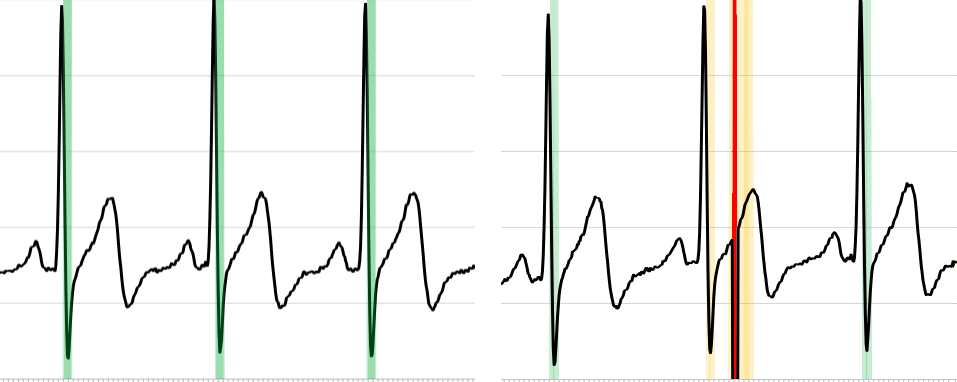
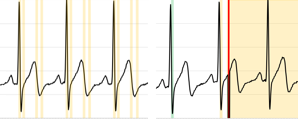
Figure 3: ECG analysis. Left: Symbolic approach, Right: Value range approach. Green: Certain heartbeats, Yellow: Potential heartbeats, Red: Bursts of unknown values.

We exploited the ability of symbolic monitors to handle assumptions by encoding that heartbeats must be apart from each other more than 160 steps (roughly $0.5$ seconds), which increased the accuracy. In one example (Fig. 0.C.8 in appendix 0.C) the monitor correctly detected a peak right after a burst of errors. The assumption allows the monitor to infer that the unknown burst of values are below a certain threshold, which enables the detection of the next heartbeat. If instead of the assumption heartbeats that are not at least 160 steps apart were simply filtered out, future heartbeats could not be detected correctly (Fig. 0.C.8(b) in appendix 0.C), because no ranges of the values of unknown events can be deduced.

6 Conclusion

We have introduced the concept of symbolic monitoring to monitor in the presence of input uncertainties and assumptions on the system behavior. We showed theoretically and empirically that symbolic monitoring is more precise than a straightforward abstract interpretation approach, and have identified logical theories in which perfect symbolic approach can be implemented efficiently (constant monitoring). Future work includes: (1) to identify other logical theories and their combinations that guarantee perfect trace length independent monitoring; (2) to be able to anticipate verdicts ahead of time for rich data domains by unfolding the symbolic representation of the specification beyond, along the lines of [2, 19, 27] for Booleans;

Finally, we envision that symbolic monitoring can become a general, foundational approach for monitoring that will allow to explain many existing monitoring approaches as instances of the general schema.

Appendix 0.A Further Examples

Example 7

Consider again $\varphi$ in Example 1, with the prefect readings in Fig. 1(b). We show for time steps $0$, $1$, $2$ an $3$ the equations before and after evaluation and simplification, in the upper and lower rows, resp.

$$\footnotesize\begin{array}[]{|l|l|l|l|}\hline\cr 0&1&2&3\\ \hline\cr\textrm{{ld}}^{0}=3&\textrm{{ld}}^{1}=4&\textrm{{ld}}^{2}=5&\textrm{{ld}}^{2}=7\\ \textrm{{acc}}^{0}=\textrm{{ld}}^{0}&\textrm{{acc}}^{1}=\textrm{{acc}}^{0}+\textrm{{ld}}^{1}&\textrm{{acc}}^{2}=\textrm{{acc}}^{1}+\textrm{{ld}}^{2}&\textrm{{acc}}^{3}=\textrm{{acc}}^{2}+\textrm{{ld}}^{3}-\textrm{{ld}}^{0}\\ \textrm{{ok}}^{0}=\textrm{{acc}}^{0}\leq 15&\textrm{{ok}}^{1}=\textrm{{acc}}^{1}\leq 15&\textrm{{ok}}^{2}=\textrm{{acc}}^{2}\leq 15&\textrm{{ok}}^{3}=\textrm{{acc}}^{3}\leq 15\\ \hline\cr&\textrm{{ld}}^{0}=3&\textrm{{ld}}^{0}=3,\textrm{{ld}}^{1}=4&\textrm{{ld}}^{1}=4,\textrm{{ld}}^{2}=5\\ \textrm{{ld}}^{0}=3&\textrm{{ld}}^{1}=4&\textrm{{ld}}^{2}=5&\textrm{{ld}}^{3}=7\\ \textrm{{acc}}^{0}=3&\textrm{{acc}}^{1}=7&\textrm{{acc}}^{2}=12&\textrm{{acc}}^{3}=16\\ \textrm{{ok}}^{0}=\textrm{{tt}}&\textrm{{ok}}^{1}=\textrm{{tt}}&\textrm{{ok}}^{2}=\textrm{{tt}}&\textrm{{ok}}^{3}=\textrm{{ff}}\\ \hline\cr\end{array}$$

All equations are fully resolved at every step. Also, $\textrm{{ld}}^{0}$ is pruned at 3 because $\textrm{{ld}}^{0}$ will not be used in the future. Consider now the imperfect input in Fig.1(d):

$$\footnotesize\begin{array}[]{|l|l|l|l|}\hline\cr 0&1&2&3\\ \hline\cr 1\leq\textrm{{ld}}^{0}\leq{}5&\textrm{{ld}}^{1}=4&\textrm{{ld}}^{2}=5&\textrm{{ld}}^{2}=7\\ \textrm{{acc}}^{0}=\textrm{{ld}}^{0}&\textrm{{acc}}^{1}=\textrm{{acc}}^{0}+\textrm{{ld}}^{1}&\textrm{{acc}}^{2}=\textrm{{acc}}^{1}+\textrm{{ld}}^{2}&\textrm{{acc}}^{3}=\textrm{{acc}}^{2}+\textrm{{ld}}^{3}-\textrm{{ld}}^{0}\\ \textrm{{ok}}^{0}=\textrm{{acc}}^{0}\leq 15&\textrm{{ok}}^{1}=\textrm{{acc}}^{1}\leq 15&\textrm{{ok}}^{2}=\textrm{{acc}}^{2}\leq 15&\textrm{{ok}}^{3}=\textrm{{acc}}^{3}\leq 15\\ \hline\cr 1\leq\textrm{{ld}}^{0}\leq{}5&\textrm{{ld}}^{1}=4&\textrm{{ld}}^{2}=5&\textrm{{ld}}^{3}=7\\ &1\leq\textrm{{ld}}^{0}\leq{}5&1\leq\textrm{{ld}}^{0}\leq{}5,\textrm{{ld}}^{1}=4&\textrm{{ld}}^{1}=4,\textrm{{ld}}^{2}=5\\ \textrm{{acc}}^{0}=\textrm{{ld}}^{0}&\textrm{{acc}}^{1}=\textrm{{ld}}^{0}+4&\textrm{{acc}}^{2}=\textrm{{ld}}^{0}+9&\textrm{{acc}}^{3}=16\\ \textrm{{ok}}^{0}=\textrm{{tt}}&\textrm{{ok}}^{1}=\textrm{{tt}}&\textrm{{ok}}^{2}=\textrm{{tt}}&\textrm{{ok}}^{3}=\textrm{{ff}}\\ \hline\cr\end{array}$$

At time $2$, $\textrm{{ok}}^{2}=\textrm{{tt}}$ is inferred from $\{1\leq\textrm{{ld}}^{0}\leq{}5,\textrm{{ld}}^{1}=4,\textrm{{acc}}^{2}=\textrm{{ld}}^{0}+9,\textrm{{ok}}^{2}=\textrm{{acc}}^{2}\leq 15\}$. At time $3$ the dependency to the unknown value $\textrm{{ld}}^{0}$ is eliminated from $\textrm{{acc}}^{3}=\textrm{{acc}}^{2}+\textrm{{ld}}^{2}-\textrm{{acc}}^{0}$ by symbolic manipulation.∎

Appendix 0.B Missing Proofs

Theorem 0.B.1

Given a specification $\varphi$ and a constant pruning strategy $\mathcal{P}$ for $\textit{Expr}^{\mathbb{B}}_{\varphi}$, there is an atemporal constant-memory monitor $M_{\varphi}$ s.t.

• $M_{\varphi}$ is sound if the pruning strategy is sound.

• $M_{\varphi}$ is perfect if the pruning strategy is perfect.

Proof

Let $\varphi=(I,O,E)$ be the atemporal specification.

We will show the theorem by constructing a monitor that generates expression sets which satisfy the relation to $\Phi^{i}$ demanded in Definition 4.

In general a monitor $M$ is perfect with respect to $\varphi$, if it generates $M^{i}$, s.t. $\llbracket\Phi^{i}\rrbracket_{{\mathbin{\mathcal{R}}}^{i}}=\llbracket M^{i}\rrbracket_{{\mathbin{\mathcal{R}}}^{i}}$ and sound, if it generates $M^{\prime i}$, s.t. $\llbracket\Phi^{i}\rrbracket_{{\mathbin{\mathcal{R}}}^{i}}\subseteq\llbracket M^{i}\rrbracket_{{\mathbin{\mathcal{R}}}^{i}}$ with ${\mathbin{\mathcal{R}}}^{i}=\{x^{i}|x\in I\cup O\}$, the relevant variables for this timestamp. This follows directly from Definition 4 and Definition 5.

We first consider the case where the pruning strategy $\mathcal{P}$ (we write $\mathcal{P}^{i}$ for the pruning according to ${\mathbin{\mathcal{R}}}^{i}$) is sound:

By using $\mathcal{P}$ we can construct a sound monitor $M$ which generates outputs $M^{0}=\mathcal{P}^{0}(\llbracket\varphi\rrbracket_{\textit{sym}}^{0}\cup\llbracket A(0)\rrbracket_{\varphi}\cup\psi^{0})$ and $M^{i}=\mathcal{P}^{i}(M^{i-1}\cup\llbracket\varphi\rrbracket_{\textit{sym}}^{i}\cup\llbracket A^{i}\rrbracket_{\varphi}\cup\psi^{i})$ for $i>0$.
We will now show $\llbracket\Phi^{i}\rrbracket_{{\mathbin{\mathcal{R}}}^{i}}\subseteq\llbracket M^{i}\rrbracket_{{\mathbin{\mathcal{R}}}^{i}}$ for all $i$, i.e. that $M$ is sound. Afterwards we will argue $M$ is also a constant-memory monitor.

For $i=0$:
By Definition 5: $\llbracket\Phi^{0}\rrbracket_{{\mathbin{\mathcal{R}}}^{0}}\subseteq\llbracket\mathcal{P}^{0}(\Phi^{0})\rrbracket_{{\mathbin{\mathcal{R}}}^{0}}$.
And by Definition of $\Phi^{0}$: $\llbracket\mathcal{P}^{0}(\Phi^{0})\rrbracket_{{\mathbin{\mathcal{R}}}^{0}}=\llbracket\mathcal{P}(\llbracket\varphi\rrbracket_{\textit{sym}}^{0}\cup\llbracket A(0)\rrbracket_{\varphi}\cup\psi^{0})\rrbracket_{{\mathbin{\mathcal{R}}}^{0}}=\llbracket M^{0}\rrbracket_{{\mathbin{\mathcal{R}}}^{0}}$.

Further, for $i>0$:
$\llbracket\Phi^{i}\rrbracket_{{\mathbin{\mathcal{R}}}^{i}}=\llbracket\Phi^{i-1}\cup\llbracket\varphi\rrbracket_{\textit{sym}}^{i}\cup\llbracket A^{i}\rrbracket_{\varphi}\cup\psi^{i}\rrbracket_{{\mathbin{\mathcal{R}}}^{i}}\subseteq\llbracket M^{i-1}\cup\llbracket\varphi\rrbracket_{\textit{sym}}^{i}\cup\llbracket A^{i}\rrbracket_{\varphi}\cup\psi^{i}\rrbracket_{{\mathbin{\mathcal{R}}}^{i}}$.
This is because of the atemporality of the monitor and the flattened form of the specification all common variables of $\Phi^{i-1}$ and $\llbracket\varphi\rrbracket_{\textit{sym}}^{i}\cup\llbracket A^{i}\rrbracket_{\varphi}\cup\psi^{i}$ are from ${\mathbin{\mathcal{R}}}^{i-1}$ for which $\llbracket M^{i-1}\rrbracket_{{\mathbin{\mathcal{R}}}^{i-1}}$ is known to be a superset of $\llbracket\Phi^{i-1}\rrbracket_{{\mathbin{\mathcal{R}}}^{i-1}}$. Hence if for any $\alpha$ we have $\alpha\models\llbracket\varphi\rrbracket_{\textit{sym}}^{i}\cup\llbracket A^{i}\rrbracket_{\varphi}\cup\psi^{i}$ and $\alpha\models\Phi^{i-1}$ then also $\alpha\models M^{i-1}$. Thus, if $\alpha\models\Phi^{i-1}\cup\llbracket\varphi\rrbracket_{\textit{sym}}^{i}\cup\llbracket A^{i}\rrbracket_{\varphi}\cup\psi^{i}$ then $\alpha\models M^{i-1}\cup\llbracket\varphi\rrbracket_{\textit{sym}}^{i}\cup\llbracket A^{i}\rrbracket_{\varphi}\cup\psi^{i}$. This fact together with the definition of $\llbracket\cdot\rrbracket_{{\mathbin{\mathcal{R}}}^{i}}$ (Definition 5) implies the subset relation above.
Furthermore $\llbracket\Phi^{i}\rrbracket_{{\mathbin{\mathcal{R}}}^{i}}\subseteq\llbracket\mathcal{P}^{i}(M^{i-1}\cup\llbracket\varphi\rrbracket_{\textit{sym}}^{i}\cup\llbracket A^{i}\rrbracket_{\varphi}\cup\psi^{i})\rrbracket_{{\mathbin{\mathcal{R}}}^{i}}=\llbracket M^{i}\rrbracket_{{\mathbin{\mathcal{R}}}^{i}}$ again by definition of $\mathcal{P}^{i}$ (Definition 5).
Hence, for all outputs of $M$ we have $\llbracket\Phi^{i}\rrbracket_{{\mathbin{\mathcal{R}}}^{i}}\subseteq\llbracket M^{i}\rrbracket_{{\mathbin{\mathcal{R}}}^{i}}$ for all $i$ and thus $M$ is sound.

Note that for all $M^{i}$ we have $|M^{i}|\leq c$ due to the constant pruning strategy. However $M$ only has to store the $M^{i}$ from the last step and as consequence it is constant-memory monitor.

The case where the pruning strategy $\mathcal{P}$ is perfect is analogous. ∎

Lemma 1

The $\textrm{Lola}_{\mathbb{B}}$ pruning strategy is perfect and constant.

Proof

Let $\mathcal{C}$ be any constraint set over $\mathcal{V}=\{s_{1},\dots,s_{n}\}\cup{\mathbin{\mathcal{R}}}$ with relevant variables $\mathcal{R}=\{r_{1},\dots,r_{m}\}$ and $\mathcal{C}^{\prime}$ the set obtained after pruning.

Clearly $\llbracket\mathcal{C}\rrbracket_{\mathbin{\mathcal{R}}}=\llbracket\mathcal{C}^{\prime}\rrbracket_{\mathbin{\mathcal{R}}}$ since by definition $\llbracket\mathcal{C}\rrbracket_{\mathbin{\mathcal{R}}}=\{(v_{1},\dots,v_{n})|(r_{1}=v_{1})\land\dots\land(r_{n}=v_{n})\models\mathcal{C}\}$. We only add value combinations to $T$ which fulfill $(r_{1}=v_{1})\land\dots\land(r_{m}=v_{m})\models\gamma$ and the $\psi_{i}$ in $\mathcal{C}^{\prime}$ by definition just allow exactly these combinations.

Moreover, the value table from which $\mathcal{C}^{\prime}$ is created has $m$ rows and $c$ columns.
Hence $\mathcal{C}^{\prime}$ contains $m$ formulas over at most $\lceil\log(c)\rceil$ variables.
According to our measure we have for every $r_{i}=\psi_{i}$ from $\mathcal{C}^{\prime}$ $|r_{i}=\psi_{i}|=1+|\psi_{i}|\leq 1+\lceil\log(c)\rceil*2^{\lceil\log(c)\rceil}\leq c^{2}+1$ and consequently $|\mathcal{C}^{\prime}|\leq m*(c^{2}+1)$.
Note that for $c$ we have $c\leq 2^{m}$ (number of columns in the table) and $m$ is the number of streams in the flattened specification and hence constant.∎

Lemma 2

The $\textrm{Lola}_{\mathcal{LA}}$ pruning strategy is perfect and constant.

Proof

Let $\mathcal{C}$ be any constraint set over $\mathcal{V}=\{s_{1},\dots,s_{n}\}\cup{\mathbin{\mathcal{R}}}$ with relevant variables $\mathcal{R}=\{r_{1},\dots,r_{m}\}$ and $\mathcal{C}^{\prime}$ the set obtained after pruning.

The strategy is clearly perfect. If $\mathcal{C}$ did not have solutions we return a $\mathcal{C}^{\prime}$ which also has no solutions. If $\mathcal{C}$ has solutions we use equivalence transformations of the system of equations preserving the solutions for $(r_{1},\dots,r_{m})$, hence $\llbracket\mathcal{C}\rrbracket_{\mathbin{\mathcal{R}}}=\{(v_{1},\dots,v_{n})|(r_{1}=v_{1})\land\dots\land(r_{n}=v_{n})\models\mathcal{C}\}=\llbracket\mathcal{C}^{\prime}\rrbracket_{\mathbin{\mathcal{R}}}$.

Note that $N^{\prime}$ is an $m\times r$ matrix with $r\leq m$. Hence in $\mathcal{C}^{\prime}$ there are $m$ expressions of the form $r_{i}=\sum_{j=1}^{r}c_{i,j}v_{j}+c_{i}$ with $|r_{i}=\sum_{j=1}^{r}c_{i,j}v_{j}+c_{i}|=2r+2$ and hence $|\mathcal{C}^{\prime}|=m*(2r+2)\leq 2m^{2}+2m$. The value $m$ is the number of streams in the flattened specification and hence constant.∎

Lemma 3

The $\textrm{Lola}_{\mathbb{B}/\mathcal{LA}}$ pruning strategy is sound and constant.

Proof

Let $\mathcal{C}$ be any constraint set over $\mathcal{V}=\{s_{1},\dots,s_{n}\}\cup{\mathbin{\mathcal{R}}}$ with relevant variables $\mathbin{\mathcal{R}}=\{r_{1},\dots,r_{m}\}$ and $\mathcal{C}^{\prime}$ the set obtained after pruning.

It follows from Lemma 1 that $\mathcal{C}^{\prime}_{\mathbb{B}}$ is a perfect pruning of $\mathcal{C}$ for ${\mathbin{\mathcal{R}}}_{\mathbb{B}}$ and from Lemma 2 that $\mathcal{C}^{\prime}_{\mathbb{R}}$ is a perfect pruning of $\mathcal{C}^{\mathcal{LE}}$ for ${\mathbin{\mathcal{R}}}_{\mathbb{R}}$.
Since $\mathcal{C}\cup\mathcal{C}^{\prime}_{\mathbb{R}}\models\{l_{i}\leq v_{i}\leq g_{i}|1\leq i\leq k\}$ by definition of $l_{i},g_{i}$, we have: $\llbracket\mathcal{C}^{\prime}\rrbracket_{\mathbin{\mathcal{R}}}=\llbracket\mathcal{C}^{\prime}_{\mathbb{B}}\cup\mathcal{C}^{\prime\prime}_{\mathbb{R}}\rrbracket_{\mathbin{\mathcal{R}}}=\llbracket\mathcal{C}^{\prime}_{\mathbb{B}}\cup\mathcal{C}^{\prime}_{\mathbb{R}}\cup\{l_{i}\leq v_{i}\leq g_{i}|1\leq i\leq k\}\rrbracket_{\mathbin{\mathcal{R}}}\supseteq\llbracket\mathcal{C}^{\prime}_{\mathbb{B}}\cup\mathcal{C}^{\prime}_{\mathbb{R}}\cup\mathcal{C}\rrbracket_{\mathbin{\mathcal{R}}}$.

We also have that, $\mathcal{C}^{\prime}_{\mathbb{B}}$ and $\mathcal{C}$ only share the variables ${\mathbin{\mathcal{R}}}_{\mathbb{B}}$ (because our pruning strategy for $\textrm{Lola}_{\mathbb{B}}$ pruned all others away and only introduced fresh variables). Furthermore $\llbracket\mathcal{C}^{\prime}_{\mathbb{B}}\rrbracket_{\mathbin{\mathcal{R}}_{\mathbb{B}}}=\llbracket\mathcal{C}\rrbracket_{\mathbin{\mathcal{R}}_{\mathbb{B}}}$. Thus it follows for all expressions $\alpha$ over $\mathbin{\mathcal{R}}$, that if $\alpha\models\mathcal{C}$ then $\alpha\models\mathcal{C}^{\prime}_{\mathbb{B}}$.
The same reasoning holds for $\mathcal{C}^{\prime}_{\mathbb{R}}$ and $\mathcal{C}$, i.e. $\alpha\models\mathcal{C}$ then $\alpha\models\mathcal{C}^{\prime}_{\mathbb{R}}$ for all expressions $\alpha$ over $\mathbin{\mathcal{R}}$.
Hence, it follows: $\llbracket\mathcal{C}^{\prime}_{\mathbb{B}}\cup\mathcal{C}^{\prime}_{\mathbb{R}}\cup\mathcal{C}\rrbracket_{\mathbin{\mathcal{R}}}\supseteq\llbracket\mathcal{C}\rrbracket_{\mathbin{\mathcal{R}}}$: The $\textrm{Lola}_{\mathbb{B}/\mathcal{LA}}$ pruning strategy is sound.

Moreover, the pruning strategy is also constant: From Lemmas 1 and 2 , $\mathcal{C}^{\prime}_{\mathbb{B}}$ and $\mathcal{C}^{\prime}_{\mathbb{R}}$ have constant upper bounds. The number of fixed-sized constraints added in step 3 is bounded by the number of fresh variables in the $\textrm{Lola}_{\mathcal{LA}}$ pruning strategy which is bounded by $m$. The value $m$ is the number of streams in the flattened specification and hence constant. Thus the size of $\mathcal{C}^{\prime}$ has a constant upper bound as well.∎

Appendix 0.C Graphs from evaluation runs

linecolor=red,backgroundcolor=red!25,bordercolor=red]Hannes: Feel free to remove some figures again if you do not like them

0.C.1 Emission Monitoring: Verdicts for uncertain inputs

Figure Monitoring trip_valid for two traces with 1% to 20% of values uncertain (range of $\pm 1\%$ to $\pm 20\%$ around correct value). Green: certain result; red: uncertain result.

0.C.2 ECG (symbolic), Full run for uncertain inputs

Figure ECG analysis 20% of the values uncertain (range of $\pm 20\%$ around correct value). Symbolic approach. Green: heartbeat certainly detected; yellow: heartbeat possibly detected.

0.C.3 ECG (intervals), Full run for uncertain inputs

Figure ECG analysis 5% of the values uncertain (range of $\pm 20\%$ around correct value). Interval approach. Green: heartbeat certainly detected; yellow: heartbeat possibly detected.

0.C.4 ECG (symbolic), Full run for 5 uncertainty bursts

Figure ECG analysis with 5 bursts of fully uncertain values(5 to 20 in a row). Symbolic approach. Orange: Burst of uncertain values; green: heartbeat certainly detected; yellow: heartbeat possibly detected.

0.C.5 ECG (intervals), Full run for 5 uncertainty bursts

Figure ECG analysis with 5 bursts of fully uncertain values(5 to 20 in a row). Interval approach. Orange: Burst of uncertain values; green: heartbeat certainly detected; yellow: heartbeat possibly detected.

0.C.6 ECG (symbolic), Full run for 5 uncertainty bursts (with assumption)

Figure ECG analysis with 5 bursts of fully uncertain values(5 to 20 in a row). Symbolic approach with assumption. Orange: Burst of uncertain values, green: heartbeat certainly detected, yellow: heartbeat possibly detected.

0.C.7 ECG (symbolic), Full run for 5 uncertainty bursts (with filter)

Figure ECG analysis with 5 bursts of fully uncertain values(5 to 20 in a row). Symbolic approach with filter. Orange: Burst of uncertain values; green: heartbeat certainly detected; yellow: heartbeat possibly detected.

0.C.8 ECG (symbolic), Bursts: Comparison Assumptions and Filter

Figure ECG analysis with bursts. Left: Usage of assumption. Right: Additional condition added to output stream. Orange: Burst of uncertain values; green: heartbeat certainly detected; yellow: heartbeat possibly detected.

References

- [1] Bartocci, E., Falcone, Y. (eds.): Lectures on Runtime Verification - Introductory and Advanced Topics, LNCS, vol. 10457. Springer (2018)
- [2] Bauer, A., Leucker, M., Schallhart, C.: Monitoring of real-time properties. In: Proc. of FSTTCS’06. LNCS, vol. 4337, pp. 260–272. Springer (2006)
- [3] Bauer, A., Leucker, M., Schallhart, C.: Comparing LTL semantics for runtime verification. J. Logic and Computation 20(3), 651–674 (2010)
- [4] Biere, A., Cimatti, A., Clarke, E.M., Strichman, O., Zhu, Y.: Bounded model checking. In: Highly Dependable Soft., chap. 3, pp. 118–149. No. 58 in Adv. in Comp., Acad. Press (2003)
- [5] Biewer, S., Finkbeiner, B., Hermanns, H., Köhl, M.A., Schnitzer, Y., Schwenger, M.: RTLola on board: Testing real driving emissions on your phone. In: Proc. TACAS’21, Part II. LNCS, vol. 12652, pp. 365–372. Springer (2021)
- [6] Cimatti, A., Tian, C., Tonetta, S.: Assumption-based runtime verification of infinite-state systems. In: Proc. of RV’21. LNCS, vol. 12974, pp. 207–227. Springer (2021)
- [7] Convent, L., Hungerecker, S., Leucker, M., Scheffel, T., Schmitz, M., Thoma, D.: TeSSLa: Temporal stream-based specification language. In: Proc. of SBMF’18. LNCS, vol. 11254, pp. 144–162. Springer (2018)
- [8] Cousot, P., Cousot, R.: Abstract interpretation: A unified lattice model for static analysis of programs by construction or approximation of fixpoints. In: POPL. pp. 238–252. ACM (1977)
- [9] D’Angelo, B., Sankaranarayanan, S., Sánchez, C., Robinson, W., Finkbeiner, B., Sipma, H.B., Mehrotra, S., Manna, Z.: LOLA: runtime monitoring of synchronous systems. In: Proc. of TIME’05. pp. 166–174. IEEE Computer Society (2005)
- [10] Decker, N., Leucker, M., Thoma, D.: Monitoring mod. theories. STTT 18(2), 205–225 (2016)
- [11] Gorostiaga, F., Sánchez, C.: Nested monitors: Monitors as expressions to build monitors. In: Proc. of RV’21. LNCS, vol. 12974, pp. 164–183. Springer (2021)
- [12] Gorostiaga, F., Sánchez, C.: Stream runtime verification of real-time event streams with the Striver language. STTT 23(2), 157–183 (2021)
- [13] Havelund, K., Goldberg, A.: Verify your runs. In: Proc. of VSTTE’05. pp. 374–383. LNCS 4171, Springer (2005)
- [14] Havelund, K., Peled, D.: An extension of first-order LTL with rules with application to runtime verification. STTT 23(4), 547–563 (2021)
- [15] Henzinger, T.A., Saraç, N.E.: Monitorability under assumptions. In: Proc. of RV’20. LNCS, vol. 12399, pp. 3–18. Springer (2020)
- [16] Kauffman, S., Havelund, K., Fischmeister, S.: What can we monitor over unreliable channels? STTT pp. 1–24 (2020)
- [17] King, J.C.: Symbolic execution and program testing. CACM 19(7), 385–394 (1976)
- [18] Köhl, M.A., Hermanns, H., Biewer, S.: Efficient monitoring of real driving emissions. In: Proc. of RV’18. LNCS, vol. 11237, pp. 299–315. Springer (2018)
- [19] Leucker, M.: Sliding between model checking and runtime verification. In: Proc. of RV’12. LNCS, vol. 7687, pp. 82–87. Springer (2012)
- [20] Leucker, M., Sánchez, C., Scheffel, T., Schmitz, M., Schramm, A.: Tessla: runtime verif. of non-synchronized real-time streams. In: SAC’18. pp. 1925–1933. ACM (2018)
- [21] Leucker, M., Sánchez, C., Scheffel, T., Schmitz, M., Thoma, D.: Runtime verif. for timed event streams with partial info. In: RV’19. LNCS, vol. 11757, pp. 273–291. Springer (2019)
- [22] Leucker, M., Schallhart, C.: A brief account of runtime verification. J. Log. Algebraic Methods Program. 78(5), 293–303 (2009)
- [23] de Moura, L.M., Bjørner, N.: Z3: An efficient SMT solver. In: Proc. of TACAS’08. LNCS, vol. 4963, pp. 337–340. Springer (2008)
- [24] Pan, J., Tompkins, W.J.: A real-time QRS detection algorithm. IEEE Trans. on Biomedical Engineering BME-32(3), 230–236 (1985)
- [25] Pnueli, A.: The temporal logic of programs. In: FOCS’77. pp. 46–57. IEEE (1977)
- [26] Sznajder, M., Łukowska, M.: Python Online and Offline ECG QRS Detector based on the Pan-Tomkins algorithm (Jul 2017)
- [27] Zhang, X., Leucker, M., Dong, W.: Runtime verification with predictive semantics. In: Proc. of NFM’12. LNCS, vol. 7226, pp. 418–432. Springer (2012)