Finite Element Method for a Nonlinear PML Helmholtz Equation
with High Wave Number

Abstract

A nonlinear Helmholtz equation (NLH) with high wave number and Sommerfeld radiation condition is approximated by the perfectly matched layer (PML) technique and then discretized by the linear finite element method (FEM). Wave-number-explicit stability and regularity estimates and the exponential convergence are proved for the nonlinear truncated PML problem. Preasymptotic error estimates are obtained for the FEM, where the logarithmic factors in $h$ required by the previous results for the NLH with impedance boundary condition are removed in the case of two dimensions. Moreover, local quadratic convergences of the Newton’s methods are derived for both the NLH with PML and its FEM. Numerical examples are presented to verify the accuracy of the FEM, which demonstrate that the pollution errors may be greatly reduced by applying the interior penalty technique with proper penalty parameters to the FEM. The nonlinear phenomenon of optical bistability can be successfully simulated.

Key words. Nonlinear Helmholtz equation, high wave number, perfectly matched layer, Newton’s method, finite element method, preasymptotic error estimates.

AMS subject classifications. 65N12, 65N15, 65N30, 78A40

1 Introduction

We are mainly concerned in this work with the following nonlinear Helmholtz equation (NLH) which may model some optical wave scattering by a nonlinear medium with a Kerr-type nonlinearity [4, 36, 17]:

(1.1) $$-\Delta u-k^{2}u-k^{2}\varepsilon{\bf 1}_{\Omega_{0}}\left|u+u_{\rm inc}\right|^{2}(u+u_{\rm inc}) =f \text{in }\mathbb{R}^{d}\;(d=2,3),$$

(1.2) $$\left|\frac{\partial u}{\partial r}-{\rm\mathbf{i}}ku\right| =o(r^{\frac{1-d}{2}}) \text{as }r=\left|x\right|\to\infty,$$

where the scattered wave $u$ is a component of the electric field, $u_{\rm inc}$ denotes the incident wave, $k\gg 1$ is the wave number, $\Omega_{0}\subset\Omega$ is the region occupied by the Kerr medium, ${\bf 1}_{\Omega_{0}}$ is the characteristic function of $\Omega_{0}$, and $\varepsilon$ is called the Kerr constant satisfying $0<\varepsilon\ll 1$, defined by $\varepsilon=4n_{2}/n_{0}$ with $n_{0}$ and $n_{2}$ to be the linear and the second-order indices of refraction, respectively. Both $n_{0}$ and $n_{2}$ are assumed real so that the medium is transparent or lossless. (1.2) is the Sommerfeld radiation condition, which ensures that the scattered wave is only outgoing. In general, $f:\mathbb{R}^{d}\to\mathbb{C}$ is an $L^{2}$ function depending on the source and the incident wave, namely, $f=f_{0}+\Delta u_{\rm inc}+k^{2}u_{\rm inc}$ with some source term $f_{0}$. Obviously, the total field $U:=u+u_{\rm inc}$ satisfies the equation

(1.3) $$-\Delta U-k^{2}U-k^{2}\varepsilon{\bf 1}_{\Omega_{0}}\left|U\right|^{2}U=f_{0}\quad\mbox{in }\mathbb{R}^{d}.$$

We suppose that $f$ is compactly supported, that is, $\mathrm{supp}\,f\subset\Omega$, where $\Omega=\mathcal{B}_{R}$ is a ball centered at the origin with radius $R$. For simplicity, we assume that the wave number $k$ is constant in the whole space $\mathbb{R}^{d}$. We write $\Gamma:=\partial\Omega$, and often have $\mathrm{dist}\,(\Gamma,\Omega_{0})\geq C\mathrm{diam}\,(\Omega_{0})$ for some constant $C$.

For numerical solutions, we should approximate the system (1.1)–(1.2) on a bounded domain. The PML technique is an efficient and very popular mesh termination technique in computational wave propagation, which was originally proposed by Bérenger [3]. The key idea is to surround $\Omega$ by a specially designed layer which can strongly absorb the outgoing waves entering the layer. Since the outgoing waves are strongly absorbed by PML, it is natural to truncate the scattered field by the simplest homogeneous Dirichlet boundary condition after an appropriate distance from the region $\Omega$, say, at $r=\hat{R}$ for some $\hat{R}>R$, as the outgoing waves would be sufficiently small there. For the linear Helmholtz equation, existing studies (see, e.g., [8, 9, 5, 26, 2, 24]) indicate that the truncated PML solution converges exponentially when the width of the layer or the PML parameter tends to infinity. In particular, Li and Wu [26] proved some wave-number-explicit stability and convergence estimates for the linear Helmholtz equation with truncated PML on the whole computational domain $\mathcal{D}:=\mathcal{B}_{\hat{R}}$ including the PML region between $\Gamma$ and $\hat{\Gamma}:=\partial\mathcal{D}$ (see Figure 1.1).

Fig. 1.1: Setting of the nonlinear PML problem.

It is well-known that when solving the wave scattering problems in high frequency, the FEMs of fixed order may suffer the so-called pollution effect, that is, its performance decreases as the wave number increases [1]. It is of significance in the theory and practical applications of FEMs to derive an error estimate containing the pollution error, namely, the preasymptotic error estimate. For preasymptotic error estimates of FEMs for the linear Helmholtz equations we refer to [22, 23, 38, 35, 14] for the impedance boundary condition and [26, 7] for the PML boundary condition. Melenk and Sauter [28, 29] showed that the $hp$-FEM is pollution free if its order is allowed to vary with the wave number $k$ (i.e. proportional to $\ln k$).

Contrary to the aforementioned rich references for linear Helmholtz equations with high wave number, we are not aware of rigorous mathematical and finite element studies of the NLH system (1.1) in the literature. We were the first time to carry out in [36] a systematical mathematical and numerical study of the NLH system with impedance boundary condition. The well-posedness of both the NLH system and its linear finite element approximation was established. Particularly, the stability estimates of the continuous NLH solutions and their finite element solutions were achieved with explicit dependence on the wave number, and the preasymptotic optimal error estimates of the finite element solutions were also derived.

The purpose of this paper is to extend the results in our early work in [36] to the practically more important case, i.e., the NLH (1.1) with PML boundary condition. Note that PML is a much more accurate approximation to the radiation condition (1.2) than the impedance boundary condition so that we can use smaller computational domain to truncate the unbounded domain and hence significantly save the computational cost. Our key idea is to introduce the Newton’s sequences of approximate linearized problems to the continuous NLH problem with PML and its FEM, respectively, and then establish the convergence of the two sequences and the preasymptotic error estimates between them. It is noted that those estimates in [36] are based on the simplest iteration, that is, the frozen-nonlinearity method, while in this paper, we consider the Newton’s method [37] and give its corresponding estimates, in particular, its quadratic convergence. Specifically, for the NLH with PML, we shall derive the wave-number-explicit stability and regularity estimates as well as the exponential convergence of its solution, under the condition that $\max\big{\{}k^{d-2}\varepsilon M(f)^{2},~{}k\varepsilon\left\|u_{\rm inc}\right\|_{L^{\infty}(\Omega_{0})}^{2}\big{\}}$ is sufficiently small and some other mild conditions on the PML parameters (see (3.2)), where $M(f)=\left\|f\right\|_{0,\Omega}+k^{2}\varepsilon\left\|u_{\rm inc}\right\|_{L^{6}(\Omega_{0})}^{3}$. Furthermore, we establish the stability and preasymptotic error estimates when the linear FEM is used to approximate the NLH with PML, under the conditions that $k^{3}h^{2}$ and $\max\big{\{}k^{d-2}\varepsilon\left|\ln h\right|^{2\bar{d}}M(f)^{2},~{}k\varepsilon\left\|u_{\rm inc}\right\|_{L^{\infty}(\Omega_{0})}^{2}\big{\}}$ are sufficiently small and the same conditions (3.2) on the PML parameters, where $\bar{d}=0$ for $d=2$ and $\bar{d}=1$ for $d=3$. The fact that $\bar{d}=0$ for $d=2$ indicates the condition on $\varepsilon$ for the FEM do not contain a logarithmic factor in $h$ in two dimensions, which is the same as that for the original NLH and improves the condition in our previous work [36] with impedance boundary condition. Moreover, we present numerical examples to verify the accuracy of the FEM, most importantly, to demonstrate that the pollution error may be greatly reduced by applying the continuous interior penalty finite element method (CIP-FEM) [13, 38, 35, 14, 26] and selecting proper penalty parameters, as well as to successfully simulate the nonlinear optical phenomenon of optical bistability (see [4]) by using the CIP-FEM solved by the Newton’s method.

The rest of this paper is organized as follows. In Section 2, we introduce the nonlinear truncated PML problem for the NLH and three iterative methods for solving the PML system. Section 3 is devoted to the stability estimates and the exponential convergence of the approximate solution to the nonlinear truncated PML problem. The quadratic convergence of the Newton’s iteration for the nonlinear truncated PML problem is also achieved. In Section 4, we establish the preasymptotic error estimates of the FEM for the nonlinear truncated PML problem and the quadratic convergence of the Newton’s iteration for the nonlinear FEM, and further introduce the CIP-FEM to reduce the pollution error. In Section 5, some numerical examples are provided to verify the accuracies of the FEM and CIP-FEM, especially to recover the phenomenon of optical bistability.

Throughout the paper, $C$ is used to denote a generic positive constant that is independent of $h,\,k,\,f$, and the penalty parameters, but may depend on the PML absorbing parameter $\sigma_{0}$ and thickness $L$ at most polynomially. We also use the shorthand notations $A\lesssim B$ and $B\gtrsim A$ for the inequality $A\leq CB$. $A\eqsim B$ is a notation for the statement that $A\lesssim B$ and $A\gtrsim B$. In addition, some standard Sobolev spaces, norms and inner products associated with Helmholtz equations are adopted, as in [6, 11]. In particular, $(\cdot,\cdot)_{Q}$ and $\langle\cdot,\cdot\rangle_{e}$ denote the $L^{2}$-inner product on complex-valued $L^{2}(Q)$ and $L^{2}(e)$ spaces, respectively. For simplicity, we will write by $\left\|\cdot\right\|_{s,G}$ and $\left|\cdot\right|_{s,G}$ the norm and semi-norm of the Sobolev space $H^{s}(G)$ for any domain $G\subset\mathbb{R}^{d}$, and write by $\chi_{G}$ the characteristic function of $G$.

2 The approximate PML problem

In this section we approximate the NLH (1.1)–(1.2) by the PML technique and state three iterative methods for the derived nonlinear PML problem.

2.1 The nonlinear approximate PML problem

It is well known that the PML system can be viewed as a consequence of the original scattering problem by a complex coordinate stretching (see e.g. [10, 12]). For simplicity, we consider the circular/spherical PML with constant absorbing coefficient. Let

(2.1) $$\tilde{r}:=\int_{0}^{r}\alpha(s)ds=r\beta(r),\quad\text{with }\alpha(r)=1+{\rm\mathbf{i}}\sigma(r),~{}\beta(r)=1+{\rm\mathbf{i}}\delta(r),$$

where $\sigma(r)$ and $\delta(r)$ are given by

(2.2) $$\sigma(r)=\left\{\begin{aligned} &0,&0\leq r\leq R,\\ &\sigma_{0},&r>R,\end{aligned}\right.\qquad\delta(r)=\left\{\begin{aligned} &0,&0\leq r\leq R,\\ &\frac{\sigma_{0}(r-R)}{r},&r>R,\end{aligned}\right.$$

with $\sigma_{0}>0$ being a constant. We assume that the PML medium property $\sigma$ is constant here to simplify the theoretical analysis, even though it is possible to employ the variable PML medium properties in practice, e.g., the PML parameter can be chosen as $\sigma(r)=\sigma_{0}(\hat{R}-R)^{-m}(r-R)^{m}$ with $m\geq 1$ when $R<r\leq\hat{R}$. However, the theoretical analysis of variable PML medium properties will be much more technical and not be considered in this work. The PML equation is obtained from the Helmholtz equation (1.1) by replacing the radial coordinate $r$ by $\tilde{r}$. For example, in the case of two dimensions $(d=2)$, the Helmholtz equation (1.1) can be written in polar coordinates as follows:

(2.3) $$-\frac{1}{r}\frac{\partial}{\partial r}\left(r\frac{\partial u}{\partial r}\right)-\frac{1}{r^{2}}\frac{\partial^{2}u}{\partial\theta^{2}}-k^{2}u-k^{2}\varepsilon{\bf 1}_{\Omega_{0}}\left|u+u_{\rm inc}\right|^{2}(u+u_{\rm inc})=f.$$

Then the PML equation is given by

$$-\frac{1}{\tilde{r}}\frac{\partial}{\partial\tilde{r}}\left(\tilde{r}\frac{\partial\tilde{u}}{\partial\tilde{r}}\right)-\frac{1}{\tilde{r}^{2}}\frac{\partial^{2}\tilde{u}}{\partial\theta^{2}}-k^{2}\tilde{u}-k^{2}\varepsilon{\bf 1}_{\Omega_{0}}\left|\tilde{u}+u_{\rm inc}\right|^{2}(\tilde{u}+u_{\rm inc})=f,$$

where $\tilde{u}(r,\theta):=u(\tilde{r},\theta)$. Noting that ${\partial}/{\partial\tilde{r}}=\alpha^{-1}{\partial}/{\partial r}$ and $\tilde{r}=\beta r$, we get

$$-\frac{1}{r}\frac{\partial}{\partial r}\left(\frac{\beta r}{\alpha}\frac{\partial\tilde{u}}{\partial r}\right)-\frac{\alpha}{\beta r^{2}}\frac{\partial^{2}\tilde{u}}{\partial\theta^{2}}-\alpha\beta k^{2}\tilde{u}-k^{2}\varepsilon{\bf 1}_{\Omega_{0}}\left|\tilde{u}+u_{\rm inc}\right|^{2}(\tilde{u}+u_{\rm inc})=f.$$

We note that $\tilde{u}=u$ in $\Omega$ and is expected to decay exponentially away from $\Gamma$. Therefore the PML problem is truncated at $r=\hat{R}$, where $\tilde{u}$ is sufficiently small. Let $\hat{\Omega}=\{x\in\mathbb{R}^{d}:\left|x\right|\in(R,\hat{R})\}$ and $L:=\hat{R}-R$ denote the PML domain and its thickness, respectively. Recalling the notation $\mathcal{D}=\mathcal{B}_{\hat{R}}$ and $\hat{\Gamma}=\partial\mathcal{D}$, we arrive at the following nonlinear truncated PML problem:

(2.4) $$-\frac{1}{r}\frac{\partial}{\partial r}\left(\frac{\beta r}{\alpha}\frac{\partial\hat{u}}{\partial r}\right)-\frac{\alpha}{\beta r^{2}}\frac{\partial^{2}\hat{u}}{\partial\theta^{2}}-\alpha\beta k^{2}\hat{u}-k^{2}\varepsilon{\bf 1}_{\Omega_{0}}\left|\hat{u}+u_{\rm inc}\right|^{2}(\hat{u}+u_{\rm inc})=f\quad\mbox{in }\mathcal{D};\quad\,\hat{u}=0\quad\mbox{on }\hat{\Gamma}.$$

The nonlinear PML problem for three dimensional case in spherical coordinates can be derived in a similar way and written as (see [26] for details):

(2.5) $$-\frac{1}{r^{2}}\frac{\partial}{\partial r}\left(\frac{\beta^{2}r^{2}}{\alpha}\frac{\partial\hat{u}}{\partial r}\right)-\frac{\alpha}{r^{2}}\Delta_{S}\hat{u}-\alpha\beta^{2}k^{2}\hat{u}-k^{2}\varepsilon{\bf 1}_{\Omega_{0}}\left|\hat{u}+u_{\rm inc}\right|^{2}(\hat{u}+u_{\rm inc})=f\quad\mbox{in }\mathcal{D};\quad\,\hat{u}=0\quad\mbox{on }\hat{\Gamma},$$

where $\Delta_{S}=\frac{1}{\sin\theta}\frac{\partial}{\partial\theta}\left(\sin\theta\frac{\partial}{\partial\theta}\right)+\frac{1}{\sin^{2}\theta}\frac{\partial^{2}}{\partial\varphi^{2}}$ is the Laplace-Beltrami operator on the unit sphere.

In Cartesian coordinates, we denote by $\hat{L}$ the linear differential operator:

$$\hat{L}w:=-\nabla\cdot(A\nabla w)-Bk^{2}w,$$

where $A$ and $B$ are defined as $A=HDH^{T}$, $B=\alpha(r)\beta^{d-1}(r),$ with the matrices $D$ and $H$ given by

$$\begin{array}[]{cc}D=\begin{pmatrix}\frac{\beta(r)}{\alpha(r)}&0\\ 0&\frac{\alpha(r)}{\beta(r)}\end{pmatrix},~{}H=\begin{pmatrix}\cos\theta&-\sin\theta\\ \sin\theta&\cos\theta\end{pmatrix}&\text{for }d=2,\\ D=\begin{pmatrix}\frac{\beta^{2}(r)}{\alpha(r)}&0&0\\ 0&\alpha(r)&0\\ 0&0&\alpha(r)\end{pmatrix},~{}H=\begin{pmatrix}\sin\theta\cos\varphi&\cos\theta\cos\varphi&-\sin\varphi\\ \sin\theta\sin\varphi&\cos\theta\sin\varphi&\cos\varphi\\ \cos\theta&-\sin\theta&0\end{pmatrix}&\text{for }d=3\,.\end{array}$$

Then the nonlinear PML problems (2.4) and (2.5) can be rewritten in the unified form in $\mathbb{R}^{d}$:

(2.6) $$\hat{L}\hat{u}-k^{2}\varepsilon{\bf 1}_{\Omega_{0}}\left|\hat{u}+u_{\rm inc}\right|^{2}(\hat{u}+u_{\rm inc})=f\quad\mbox{in }\mathcal{D};\quad\,\hat{u}=0\quad\mbox{on }\hat{\Gamma}.$$

For simplicity, throughout the rest of the paper, we shall use the notations:

$$\left\|\cdot\right\|_{s}=\left\|\cdot\right\|_{s,\mathcal{D}}=\left\|\cdot\right\|_{H^{s}(\mathcal{D})},\quad\left|\cdot\right|_{s}=\left|\cdot\right|_{s,\mathcal{D}}=\left|\cdot\right|_{H^{s}(\mathcal{D})}\quad\mbox{and}\quad(\cdot,\cdot)=(\cdot,\cdot)_{\mathcal{D}}.$$

Since $A(x)$ is discontinuous across $\Gamma=\partial\Omega$, $\hat{u}$ may be not in the space $H^{2}(D)$. Note that

$$\hat{u}\in H^{2}(\Omega\cup\hat{\Omega}):=\{v\in L^{2}(\mathcal{D}):v|_{\Omega}\in H^{2}(\Omega),\;v|_{\hat{\Omega}}\in H^{2}(\hat{\Omega})\},$$

we define the corresponding norm and semi-norm by

$$\left\|\cdot\right\|_{2,\Omega\cup\hat{\Omega}}=\big{(}\left\|\cdot\right\|_{2,\Omega}^{2}+\left\|\cdot\right\|_{2,\hat{\Omega}}^{2}\big{)}^{1/2},\quad\left|\cdot\right|_{2,\Omega\cup\hat{\Omega}}=\big{(}\left|\cdot\right|_{2,\Omega}^{2}+\left|\cdot\right|_{2,\hat{\Omega}}^{2}\big{)}^{1/2}.$$

The variational formulation of the nonlinear PML problem (2.6) reads as: find $\hat{u}\in H_{0}^{1}(\mathcal{D})$ such that

(2.7) $$a^{\rm NL}(\hat{u},v)=(f,v)\quad\forall v\in H_{0}^{1}(\mathcal{D}),$$

where $a^{\rm NL}(u,v)$ is defined by

(2.8) $$a^{\rm NL}(u,v) :=a(u,v)-k^{2}\varepsilon\big{(}\left|u+u_{\rm inc}\right|^{2}(u+u_{\rm inc}),v\big{)}_{\Omega_{0}},$$

(2.9) $$a(u,v) :=(A\nabla u,\nabla v)-k^{2}(Bu,v).$$

We shall often use the following energy norm in the subsequent analysis:

(2.10) $$\left\|{\hskip-2.7pt}\left|v\right|{\hskip-2.7pt}\right\|=\Big{(}\Re\big{(}a(v,v)\big{)}+2k^{2}\left\|v\right\|_{0}^{2}\Big{)}^{1/2}\quad\forall\,v\in H^{1}(\mathcal{D})\,.$$

It can be shown that $\left\|{\hskip-2.7pt}\left|v\right|{\hskip-2.7pt}\right\|\eqsim k\left\|v\right\|_{0}+\left\|\nabla v\right\|_{0}$. In fact, noting that $0\leq\delta\leq\sigma\leq\sigma_{0}$, we have for the case of $d=2$ that

$$\left\|{\hskip-2.7pt}\left|v\right|{\hskip-2.7pt}\right\|^{2} =\Re\big{(}a(v,v)\big{)}+2k^{2}\left\|v\right\|_{0}^{2}$$

$$=\int_{0}^{2\pi}{\hskip-7.0pt}\int_{0}^{\hat{R}}\bigg{(}\frac{1+\sigma\delta}{1+\sigma^{2}}r\left|v_{r}\right|^{2}+\frac{1+\sigma\delta}{1+\delta^{2}}\frac{1}{r}\left|v_{\theta}\right|^{2}+(1+\sigma\delta)k^{2}r\left|v\right|^{2}\bigg{)}drd\theta,$$

which leads to

(2.11) $$(1+\sigma_{0}^{2})^{-1}\left\|\nabla v\right\|_{0}^{2}+k^{2}\left\|v\right\|_{0}^{2}\leq\left\|{\hskip-2.7pt}\left|v\right|{\hskip-2.7pt}\right\|^{2}\leq(1+\sigma_{0}^{2})(\left\|\nabla v\right\|_{0}^{2}+k^{2}\left\|v\right\|_{0}^{2}).$$

Similarly, we obtain for the case of $d=3$ that

$$\left\|{\hskip-2.7pt}\left|v\right|{\hskip-2.7pt}\right\|^{2}=\Re\big{(}a(v,v)\big{)}+2k^{2}\left\|v\right\|_{0}^{2}$$

$$=\int_{0}^{2\pi}{\hskip-7.0pt}\int_{0}^{\pi}{\hskip-5.0pt}\int_{0}^{\hat{R}}\sin\theta\bigg{(}\frac{1-\delta^{2}+2\sigma\delta}{1+\sigma^{2}}r^{2}\left|v_{r}\right|^{2}+\left|v_{\theta}\right|^{2}+\frac{1}{\sin^{2}\theta}\left|v_{\varphi}\right|^{2}+(1+\delta^{2}+2\sigma\delta)k^{2}r^{2}\left|v\right|^{2}\bigg{)}drd\varphi d\theta,$$

which leads to

(2.12) $$(1+\sigma_{0}^{2})^{-1}\left\|\nabla v\right\|_{0}^{2}+k^{2}\left\|v\right\|_{0}^{2}\leq\left\|{\hskip-2.7pt}\left|v\right|{\hskip-2.7pt}\right\|^{2}\leq(1+3\sigma_{0}^{2})(\left\|\nabla v\right\|_{0}^{2}+k^{2}\left\|v\right\|_{0}^{2}).$$

2.2 Iterative methods for the nonlinear PML problem

To solve the nonlinear PML problem (2.6), we introduce three iterative methods. The first and simplest one is the frozen-nonlinearity iteration:

Given initial function $\hat{u}_{0}\in H_{0}^{1}(\mathcal{D})$, find $\hat{u}^{l+1}\in H_{0}^{1}(\mathcal{D})$ for $l=0,1,2,\cdots$, such that

(2.13) $$\hat{L}\hat{u}^{l+1}-k^{2}\varepsilon{\bf 1}_{\Omega_{0}}\left|\hat{u}^{l}+u_{\rm inc}\right|^{2}(\hat{u}^{l+1}+u_{\rm inc})=f.$$

It is known that the iteration (2.13) only has the linear convergence rate and converges for problems with weak nonlinearity (see [37, 36]). The analysis of the nonlinear PML problem (2.6) based on the iteration (2.13) is similar to that of the NLH (1.3) with impedance boundary condition in [36] and is omitted here.

The second one is the Newton’s method:

Given $\hat{u}^{0}\in H_{0}^{1}(\mathcal{D})$, find $\hat{u}^{l+1}\in H_{0}^{1}(\mathcal{D})$ for $l=0,1,2,\cdots$, such that

(2.14) $$\hat{L}\hat{u}^{l+1} -k^{2}\varepsilon{\bf 1}_{\Omega_{0}}\Big{(}2\left|\hat{u}^{l}+u_{\rm inc}\right|^{2}\hat{u}^{l+1}+\big{(}\hat{u}^{l}+u_{\rm inc}\big{)}^{2}\overline{\hat{u}^{l+1}}\Big{)}$$

$$=f -k^{2}\varepsilon{\bf 1}_{\Omega_{0}}\Big{(}2\left|\hat{u}^{l}+u_{\rm inc}\right|^{2}\hat{u}^{l}-\big{(}\hat{u}^{l}+u_{\rm inc}\big{)}^{2}\overline{u_{\rm inc}}\Big{)}.$$

The Newton’s method converges not only for problems with weak nonlinearity but also for problems with strong nonlinearity and converges at a quadratic rate once the initial function $\hat{u}^{0}$ is sufficiently close to the exact solution. The Newton’s method will be analyzed in the next section.

The third one is a modified Newton’s method proposed by [37]. It is obtained by replacing $\overline{\hat{u}^{l+1}}$ in (2.14) by $\overline{\hat{u}^{l}}$ and then given by

(2.15) $$\hat{L}\hat{u}^{l+1}-2k^{2}\varepsilon{\bf 1}_{\Omega_{0}}\left|\hat{u}^{l}+u_{\rm inc}\right|^{2}\hat{u}^{l+1}=f-k^{2}\varepsilon{\bf 1}_{\Omega_{0}}\left|\hat{u}^{l}+u_{\rm inc}\right|^{2}\left(\hat{u}^{l}-u_{\rm inc}\right),\quad l\geq 0.$$

Compared with the Newton’s method, the modified Newton’s method has only linear convergence rate but numerical evidences indicate that it is robust with respect to the initial guess. The analysis of this method is left to a future work.

3 Analyses of the nonlinear PML problem

In this section, we shall present the well-posedness of the nonlinear PML problem (2.6) and prove the exponential convergence of the nonlinear PML solution to the original NLH solution. To do so, we regard the nonlinear PML solution as the limits of the sequence constructed by Newton’s iteration (2.14). We shall first derive some uniform bounds for the linearized problems and then prove the quadratic convergence of the iteration sequence.

3.1 An auxiliary linearized problem

Before analyzing the nonlinear PML problem (2.6), we study a linearized problem associated with the Newton’s iteration (2.14): for given function $\phi\in L^{\infty}(\mathcal{D})$ and $g\in L^{2}(\mathcal{D})$, $\hat{w}^{\phi}\in H^{1}_{0}(\mathcal{D})$ solves

(3.1) $$\hat{L}\hat{w}^{\phi}-k^{2}\varepsilon{\bf 1}_{\Omega_{0}}\big{(}2\left|\phi+u_{\rm inc}\right|^{2}\hat{w}^{\phi}+(\phi+u_{\rm inc})^{2}\overline{\hat{w}^{\phi}}\big{)}=g.$$

For the stability of the solution to this auxiliary linear system, we first recall some estimates of the solution to a linear Helmholtz problem and the Hankel functions of the first kind.

Lemma 3.1 ([26, Theorem 3.1 and Corollaries 3.4 and 3.9]).

For a given source $\hat{g}\in L^{2}(\mathcal{D})$, let $\hat{w}\in H_{0}^{1}(\mathcal{D})$ solve $\hat{L}\hat{w}=\hat{g}$, then under the conditions that $R\eqsim\hat{R}\eqsim 1$ and

(3.2) $$kR\geq 1\quad\mbox{and}\quad k\sigma_{0}L\geq\max\big{\{}2kR+\sqrt{3}kL,10\big{\}},$$

there exists a positive constant $C_{\mathcal{L}}$ independent of $k$ and $\hat{g}$ such that

(3.3) $$k\left\|\hat{w}\right\|_{0}+\left\|{\hskip-2.7pt}\left|\hat{w}\right|{\hskip-2.7pt}\right\|+k^{-1}\left|\hat{w}\right|_{2,\Omega\cup\hat{\Omega}}\leq C_{\mathcal{L}}\left\|\hat{g}\right\|_{0}.$$

Lemma 3.2 ([8, Lemma 2.2]).

For any $\nu\in\mathbb{R}$, $z\in\mathbb{C}_{++}=\left\{z\in\mathbb{C}:\Im(z)\geq 0,\Re(z)\geq 0\right\}$ and $0<x\leq\left|z\right|$, the following estimate holds for the Hankel function $H_{\nu}^{(1)}(z)$ of the first kind:

(3.4) $$\left|H_{\nu}^{(1)}(z)\right|\leq e^{-\Im(z)\left(1-\frac{x^{2}}{\left|z\right|^{2}}\right)^{1/2}}\left|H_{\nu}^{(1)}(x)\right|.$$

Using Lemma 3.1, we can readily get the stability estimate of the solutions to the auxiliary linear system (3.1). To do so, we rewrite it as

(3.5) $$\hat{L}\hat{w}^{\phi}=g+k^{2}\varepsilon{\bf 1}_{\Omega_{0}}\big{(}2\left|\phi+u_{\rm inc}\right|^{2}\hat{w}^{\phi}+(\phi+u_{\rm inc})^{2}\overline{\hat{w}^{\phi}}\big{)}.$$

Applying (3.3) to (3.5), we obtain

$$k\left\|\hat{w}^{\phi}\right\|_{0}+\left\|{\hskip-2.7pt}\left|\hat{w}^{\phi}\right|{\hskip-2.7pt}\right\|+k^{-1}\left|\hat{w}^{\phi}\right|_{2,\Omega\cup\hat{\Omega}} \leq C_{\mathcal{L}}\left\|g\right\|_{0}+3C_{\mathcal{L}}k^{2}\varepsilon\left\|\phi+u_{\rm inc}\right\|_{L^{\infty}(\Omega_{0})}^{2}\left\|\hat{w}^{\phi}\right\|_{0},$$

which leads to the following estimate (by taking $\theta_{0}={1}/{(24C_{\mathcal{L}})}$ there).

Lemma 3.3.

Let the conditions of Lemma 3.1 be satisfied. Then there exists a positive constant $\theta_{0}\lesssim 1$ such that the solution $\hat{w}^{\phi}$ to (3.1) satisfies

(3.6) $$k\left\|\hat{w}^{\phi}\right\|_{0}+\left\|{\hskip-2.7pt}\left|\hat{w}^{\phi}\right|{\hskip-2.7pt}\right\|+k^{-1}\left|\hat{w}^{\phi}\right|_{2,\Omega\cup\hat{\Omega}}\leq 2C_{\mathcal{L}}\left\|g\right\|_{0},$$

under the condition that $\max\{k\varepsilon\left\|\phi\right\|_{L^{\infty}(\Omega_{0})}^{2},\,k\varepsilon\left\|u_{\rm inc}\right\|_{L^{\infty}(\Omega_{0})}^{2}\}\leq\theta_{0}.$

The uniqueness of the solutions to the auxiliary linearized problem (3.1) follows directly from Lemma 3.3. Furthermore, the existence of a solution can be obtained by the uniqueness and the Fredholm alternative theorem. In fact, by writing $\hat{w}^{\phi}=\hat{w}^{\phi}_{r}+{\rm\mathbf{i}}\hat{w}^{\phi}_{i}$, where $\hat{w}^{\phi}_{r}$ and $\hat{w}^{\phi}_{i}$ are both real-valued functions, we can get an equivalent variational problem with a bilinear form defined on real-valued Sobolev spaces. Then it can be proved that the equivalent bilinear form is continuous and satisfies the Gårding’s inequality, so an application of the Fredholm alternative theorem will lead to the existence of a solution to the variational problem following from the uniqueness; see, e.g., [27, Theorem 2.34] or [15, §6.2]. Therefore, the auxiliary linearized problem (3.1) is well-posed.

Moreover, we have the following $L^{\infty}$-estimate in $\Omega_{0}$ for the solution $\hat{w}^{\phi}$ to (3.1), which will play a crucial role in our subsequent analysis.

Lemma 3.4.

Let the conditions of Lemma 3.3 be satisfied, then the solution $\hat{w}^{\phi}$ to (3.1) satisfies

(3.7) $$\left\|\hat{w}^{\phi}\right\|_{L^{\infty}(\Omega_{0})}\lesssim k^{\frac{d-3}{2}}\left\|g\right\|_{0}.$$

Proof.

The estimate (3.7) is a direct consequence of the following estimate

(3.8) $$\left\|\hat{w}\right\|_{L^{\infty}(\Omega_{0})}\lesssim k^{\frac{d-3}{2}}\left\|\hat{g}\right\|_{0},$$

where $\hat{w}\in H_{0}^{1}(\mathcal{D})$ solves the linear problem $\hat{L}\hat{w}=\hat{g}$. In fact, by rewriting the system (3.1) to (3.5), then applying the estimate (3.8) to (3.5) with $\hat{g}=g+k^{2}\varepsilon{\bf 1}_{\Omega_{0}}\big{(}2\left|\phi+u_{\rm inc}\right|^{2}\hat{w}^{\phi}+(\phi+u_{\rm inc})^{2}\overline{\hat{w}^{\phi}}\big{)}$, we obtain

$$\left\|\hat{w}^{\phi}\right\|_{L^{\infty}(\Omega_{0})} \lesssim k^{\frac{d-3}{2}}\big{(}\left\|g\right\|_{0}+k^{2}\varepsilon\left\|\phi+u_{\rm inc}\right\|_{L^{\infty}(\Omega_{0})}^{2}\left\|\hat{w}^{\phi}\right\|_{0,\Omega_{0}}\big{)}\lesssim k^{\frac{d-3}{2}}\big{(}\left\|g\right\|_{0}+2k\theta_{0}\left\|\hat{w}^{\phi}\right\|_{0,\Omega_{0}}\big{)},$$

which, together with (3.6), gives (3.7). It remains to establish (3.8).

Case 1: $d=2$. We first notice that $0\leq r=|x|\leq R_{0}:=R-\mathrm{dist}\,(\Gamma,\Omega_{0})$ for $x\in\Omega_{0}$. The solution $\hat{w}$ in $\Omega_{0}$ can be solved by separation of variables and expressed by Fourier expansions (see [26, (2.23)–(2.24)]):

(3.9) $$\hat{w}=v+w+\zeta\,\,\,\text{with}\,\,\,v=\sum_{n\in\mathbb{Z}}v_{n}(r)e^{{\rm\mathbf{i}}n\theta},\,w=\sum_{n\in\mathbb{Z}}w_{n}(r)e^{{\rm\mathbf{i}}n\theta},\,\zeta=\sum_{n\in\mathbb{Z}}\zeta_{n}(r)e^{{\rm\mathbf{i}}n\theta},$$

where the coefficients $v_{n}(r)$, $v_{n}(r)$ and $\zeta_{n}(r)$ are given by

$$v_{n}(r) =\frac{\pi{\rm\mathbf{i}}}{2}J_{n}(kr)\int_{r}^{R}H_{n}^{(1)}(kt)g_{n}(t)tdt+\frac{\pi{\rm\mathbf{i}}}{2}H_{n}^{(1)}(kr)\int_{0}^{r}J_{n}(kt)g_{n}(t)tdt,$$

$$w_{n}(r) =\frac{\pi{\rm\mathbf{i}}}{2}J_{n}(kr)\int_{R}^{\hat{R}}H_{n}^{(1)}(k\tilde{t})g_{n}(t)tdt,$$

$$\zeta_{n}(r) =\hat{C}_{n}J_{n}(kr),\quad\hat{C}_{n}=-\frac{\pi{\rm\mathbf{i}}}{2}\frac{H_{n}^{(1)}(k\tilde{\hat{R}})}{J_{n}(k\tilde{\hat{R}})}\int_{0}^{\hat{R}}J_{n}(k\tilde{t})g_{n}(t)tdt,$$

where $J_{n}$ denotes the Bessel function of the first kind with order $n$, and $g_{n}(r)=\frac{1}{2\pi}\int_{0}^{2\pi}\hat{g}(r,\theta)e^{-{\rm\mathbf{i}}n\theta}d\theta$ is the Fourier coefficient of $\hat{g}$ on $\partial\mathcal{B}_{r}$. It is easy to see that $v$ is the solution to the linear Helmholtz equation $-\Delta v-k^{2}v=\hat{g}\chi_{\Omega}$ with the Sommerfeld radiation condition (i.e. (1.2)). Thus,

$$v(x)=\int_{\mathbb{R}^{2}}\hat{g}(y)\chi_{\Omega}(y)G(x,y)dy\quad\text{for }x\in\Omega_{0},$$

where $G(x,y){=\frac{{\rm\mathbf{i}}}{4}H_{0}^{(1)}(k|x-y|)}$ denotes the standard Green’s function. From [34, p. 211], we have

$$|G(x,y)|\lesssim\frac{1}{\sqrt{k|x-y|}}\quad\mbox{and}\quad\int_{\Omega}|G(x,y)|^{2}{\rm d}y\lesssim k^{-1},$$

hence we can easily get

$$\left\|v\right\|_{L^{\infty}(\Omega_{0})}\lesssim k^{-1/2}\left\|\hat{g}\right\|_{0,\Omega}.$$

Similarly, for $x\in\Omega_{0}$, we have

$$w(x)=\int_{\mathbb{R}^{2}}\tilde{g}(y)\chi_{\hat{\Omega}}(y)G(x,y)dy,$$

where $\tilde{g}=\sum_{n\in\mathbb{N}}\tilde{g}_{n}(r)e^{{\rm\mathbf{i}}n\theta}$ and $\tilde{g}_{n}(r):=g_{n}(r)H_{n}^{(1)}(k\tilde{r})/H_{n}^{(1)}(kr)$. According to [32, §10.21(i)], the positive zeros of the two real Bessel functions $J_{n}(kr)$ and $Y_{n}(kr)$ are interlaced and hence, $H_{n}^{(1)}(kr)=J_{n}(kr)+{\rm\mathbf{i}}Y_{n}(kr)\not=0$. From Lemma 3.2, we have $\left|\tilde{g}_{n}(r)\right|\leq\left|g_{n}(r)\right|$ and then

$$\left\|w\right\|_{L^{\infty}(\Omega_{0})}\lesssim k^{-1/2}\left\|\tilde{g}\right\|_{0,\hat{\Omega}}\lesssim k^{-1/2}\left\|\hat{g}\right\|_{0,\hat{\Omega}}.$$

For the last term $\zeta=\sum_{n\in\mathbb{N}}\zeta_{n}(r)e^{{\rm\mathbf{i}}n\theta}$ in (3.9), by applying [26, (3.24) and (3.33)], we get

$$\left|\hat{C}_{n}\right|\lesssim e^{-\frac{1}{2}k\sigma_{0}L}\left(\int_{0}^{\hat{R}}r\left|g_{n}(r)\right|^{2}dr\right)^{\frac{1}{2}}.$$

Noting that $J_{0}(kr)^{2}+2\sum_{n=1}^{\infty}J_{n}(kr)^{2}=1$ (cf. [32, (10.23.3)]), we have

$$\left|\zeta\right|=\left|\sum_{n\in\mathbb{N}}\hat{C}_{n}J_{n}(kr)e^{{\rm\mathbf{i}}n\theta}\right|\leq\left(\sum_{n\in\mathbb{N}}\left|\hat{C}_{n}\right|^{2}\right)^{\frac{1}{2}}\left(\sum_{n\in\mathbb{N}}J_{n}(kr)^{2}\right)^{\frac{1}{2}}\lesssim e^{-\frac{1}{2}k\sigma_{0}L}\left\|\hat{g}\right\|_{0}.$$

Since $\sigma_{0}L\gtrsim 1$ (see (3.2)), we have $e^{-\frac{1}{2}k\sigma_{0}L}\lesssim k^{-1/2}$, then

$$\left\|\zeta\right\|_{L^{\infty}(\Omega_{0})}\lesssim e^{-\frac{1}{2}k\sigma_{0}L}\left\|\hat{g}\right\|_{0}\lesssim k^{-1/2}\left\|\hat{g}\right\|_{0}.$$

Therefore, we have confirmed the validity of (3.8) for $d=2$.

Case 2: $d=3$. The proof is similar to the case of $d=2$. From [26, (2.30)–(2.31)], $\hat{w}$ can be expressed by the harmonic expansion $\hat{w}=v+w+\zeta$ in $\Omega_{0}$, with

$$v=\sum_{l=0}^{\infty}\sum_{m=-l}^{l}v_{l}^{m}(r)Y_{l}^{m}(\theta,\varphi),\;w=\sum_{l=0}^{\infty}\sum_{m=-l}^{l}w_{l}^{m}(r)Y_{l}^{m}(\theta,\varphi),\;\zeta=\sum_{l=0}^{\infty}\sum_{m=-l}^{l}\zeta_{l}^{m}(r)Y_{l}^{m}(\theta,\varphi),$$

where $Y_{l}^{m}$ is the standard spherical harmonics (see [34, etc.]) and

$$v_{l}^{m}(r) =\frac{\pi{\rm\mathbf{i}}}{2}r^{-\frac{1}{2}}J_{\nu}(kr)\int_{r}^{R}H_{\nu}^{(1)}(kt)g_{l}^{m}(t)t^{\frac{3}{2}}dt+\frac{\pi{\rm\mathbf{i}}}{2}r^{-\frac{1}{2}}H_{\nu}^{(1)}(kr)\int_{0}^{r}J_{\nu}(kt)g_{l}^{m}(t)t^{\frac{3}{2}}dt,$$

$$w_{l}^{m}(r) =\frac{\pi{\rm\mathbf{i}}}{2}r^{-\frac{1}{2}}J_{\nu}(kr)\int_{R}^{\hat{R}}H_{\nu}^{(1)}(k\tilde{t})\beta^{-\frac{1}{2}}g_{l}^{m}(t)t^{\frac{3}{2}}dt$$

$$\zeta_{l}^{m}(r) =\hat{C}_{\nu}r^{-\frac{1}{2}}J_{\nu}(kr),\quad\hat{C}_{\nu}=-\frac{\pi{\rm\mathbf{i}}}{2}\frac{H_{\nu}^{(1)}(k\tilde{\hat{R}})}{J_{\nu}(k\tilde{\hat{R}})}\int_{0}^{\hat{R}}J_{\nu}(k\tilde{t})\beta^{-\frac{1}{2}}g_{l}^{m}(t)t^{\frac{3}{2}}dt,$$

where $\nu:=l+\frac{1}{2}$ and $g_{l}^{m}(r)=\int_{0}^{2\pi}\int_{0}^{\pi}\hat{g}(r,\theta,\varphi)Y_{l}^{-m}(\theta,\varphi)\sin\theta d\theta d\varphi$. Noting that $v$ is the solution to the linear Helmholtz equation $-\Delta v-k^{2}v=\hat{g}\chi_{\Omega}$ with Sommerfeld radiation condition. Thus,

$$v(x)=\int_{\mathbb{R}^{3}}\hat{g}(y)\chi_{\Omega}(y)G(x,y)dy,$$

where $G(x,y)=\frac{e^{{\rm\mathbf{i}}k|x-y|}}{4\pi|x-y|}$ denotes the standard Green’s function. Obviously, $\left|G(x,y)\right|\lesssim\frac{1}{|x-y|}$, then we get

$$\int_{\Omega}\left|G(x,y)\right|^{2}dy\lesssim 1,\quad\mbox{and then,}\quad\left\|v\right\|_{L^{\infty}(\Omega_{0})}\lesssim\left\|\hat{g}\right\|_{0,\Omega}.$$

Similarly, we have

$$w(x)=\int_{\mathbb{R}^{3}}\tilde{g}(y)\chi_{\hat{\Omega}}(y)G(x,y)dy,$$

where

$$\tilde{g}=\sum_{l=0}^{\infty}\sum_{m=-l}^{l}\tilde{g}_{l}^{m}(r)Y_{l}^{m}(\theta,\varphi)\quad\mbox{and}\quad\tilde{g}_{l}^{m}(r)=\beta^{-1/2}g_{l}^{m}(r)H_{\nu}^{(1)}(k\tilde{r})/H_{\nu}^{(1)}(kr).$$

Using Lemma 3.2 again, we have $\left|\tilde{g}_{l}^{m}(r)\right|\lesssim\left|g_{l}^{m}(r)\right|$ and then

$$\left\|w\right\|_{L^{\infty}(\Omega_{0})}\lesssim\left\|\tilde{g}\right\|_{0,\hat{\Omega}}\lesssim\left\|\hat{g}\right\|_{0,\hat{\Omega}}.$$

For the last term $\zeta$, from [26, (3.40)] and a similar proof to [26, (3.24)], we have

$$\left|\hat{C}_{\nu}\right|\lesssim\sqrt{k}e^{-\frac{1}{2}k\sigma_{0}L}\left(\int_{0}^{\hat{R}}r^{2}\left|g_{l}^{m}(r)\right|^{2}dr\right)^{\frac{1}{2}}.$$

Hence,

$$\left|\zeta\right| =\left|\sum_{l=0}^{\infty}\sum_{m=-l}^{l}\hat{C}_{\nu}r^{-\frac{1}{2}}J_{\nu}(kr)Y_{l}^{m}(\theta,\varphi)\right|=\left|\sum_{l=0}^{\infty}\sum_{m=-l}^{l}\hat{C}_{\nu}\sqrt{\frac{2k}{\pi}}j_{l}(kr)Y_{l}^{m}(\theta,\varphi)\right|$$

$$\lesssim ke^{-\frac{1}{2}k\sigma_{0}L}\left\|\hat{g}\right\|_{0}\left(\sum_{l=0}^{\infty}j_{l}^{2}(kr)\sum_{m=-l}^{l}\left|Y_{l}^{m}\right|^{2}\right)^{\frac{1}{2}},$$

where $j_{l}$ denotes the spherical Bessel function of the first kind and order $l$. From [30, (2.4.105)] and [32, (10.60.12)], we have

$$\sum_{m=-l}^{l}\left|Y_{l}^{m}\right|^{2}=\frac{2l+1}{4\pi}\quad\mbox{and}\quad\sum_{l=0}^{\infty}(2l+1)j_{l}^{2}(kr)=1,$$

then we arrive at

$$\left\|\zeta\right\|_{L^{\infty}(\Omega_{0})}\lesssim ke^{-\frac{1}{2}k\sigma_{0}L}\left\|\hat{g}\right\|_{0}\lesssim\left\|\hat{g}\right\|_{0},$$

where we have used $\sigma_{0}L\gtrsim 1$. Therefore, (3.8) also holds for $d=3$. ∎

Remark 3.5.

We can easily obtain the estimate from the proof of Lemma 3.4 above that

(3.10) $$\left\|\hat{w}^{\phi}\right\|_{L^{\infty}(\Omega_{1})}\lesssim k^{\frac{d-3}{2}}\left\|g\right\|_{0}$$

for any subdomain $\Omega_{1}$ satisfying $\Omega_{0}\subset\subset\Omega_{1}\subset\subset\Omega$ and $\mathrm{dist}\,(\Gamma,\partial\Omega_{1})\eqsim\mathrm{dist}\,(\partial\Omega_{1},\partial\Omega_{0})$.

3.2 Existence and stability estimates for the nonlinear PML problem

In this subsection, we study the well-posedness of the nonlinear PML problem (2.6). This is carried out by the Newton’s iterative process (2.14). We start with some uniform stability estimates for the solutions $\{\hat{u}^{l}\}_{l\geq 1}$ to (2.14) in terms of the iteration number $l$, with their bounds depending on the constant

(3.11) $$M(f):=\left\|f\right\|_{0,\Omega}+k^{2}\varepsilon\left\|u_{\rm inc}\right\|_{L^{6}(\Omega_{0})}^{3}.$$

Lemma 3.6.

Under the conditions of Lemma 3.1, there exists a positive constant $\theta_{1}\lesssim 1$ such that if

(3.12) $$k\left\|\hat{u}^{0}\right\|_{0,\Omega_{0}}\lesssim M(f),\quad\left\|\hat{u}^{0}\right\|_{L^{\infty}(\Omega_{0})}\lesssim k^{\frac{d-3}{2}}M(f),$$

(3.13) $$\max\big{\{}k^{d-2}\varepsilon M(f)^{2},~{}k\varepsilon\left\|u_{\rm inc}\right\|_{L^{\infty}(\Omega_{0})}^{2}\big{\}}\leq\theta_{1},$$

then the following estimates hold for $l=1,2,\cdots$:

(3.14) $$k\left\|\hat{u}^{l}\right\|_{0}+\left\|{\hskip-2.7pt}\left|\hat{u}^{l}\right|{\hskip-2.7pt}\right\|+k^{-1}\left|\hat{u}^{l}\right|_{2,\Omega\cup\hat{\Omega}}\lesssim M(f),\quad\left\|\hat{u}^{l}\right\|_{L^{\infty}(\Omega_{0})}\lesssim k^{\frac{d-3}{2}}M(f).$$

Proof.

We set

$$\hat{f}^{l}:= \;f-k^{2}\varepsilon{\bf 1}_{\Omega_{0}}\big{(}2|\hat{u}^{l}+u_{\rm inc}|^{2}\hat{u}^{l}-(\hat{u}^{l}+u_{\rm inc})^{2}\overline{u_{\rm inc}}\big{)}$$

$$= \;f-k^{2}\varepsilon{\bf 1}_{\Omega_{0}}\big{(}2|\hat{u}^{l}|^{2}\hat{u}^{l}+2|\hat{u}^{l}|^{2}u_{\rm inc}+(\hat{u}^{l})^{2}\overline{u_{\rm inc}}-|u_{\rm inc}|^{2}u_{\rm inc}\big{)}.$$

First, we let $C_{\mathcal{L}}$ be the constant from (3.6) and $C_{\infty}$ be the hidden generic constant in (3.7). Denote by $\widetilde{C}_{\mathcal{L}}=4C_{\mathcal{L}}$ and $\widetilde{C}_{\infty}=2C_{\infty}$ and let $\theta_{1}\leq\min\big{\{}\theta_{0},\theta_{0}/\widetilde{C}_{\infty}^{2},1/(2\widetilde{C}_{\mathcal{L}}\widetilde{C}_{\infty}^{2}+3\widetilde{C}_{\mathcal{L}}\widetilde{C}_{\infty})\big{\}}$, where $\theta_{0}$ is from Lemma 3.3. We also assume that the initial value satisfies $k\|\hat{u}^{0}\|_{0,\Omega_{0}}\leq\widetilde{C}_{\mathcal{L}}M(f)$ and $\|{\hat{u}^{0}}\|_{L^{\infty}(\Omega_{0})}\leq\widetilde{C}_{\infty}k^{\frac{d-3}{2}}M(f)$.

Next, we suppose that the following estimates hold for $l=n$ with $n\geq 0$:

$$k\big{\|}\hat{u}^{n}\big{\|}_{0,\Omega_{0}}\leq\widetilde{C}_{\mathcal{L}}M(f)\quad\mbox{and}\quad\big{\|}\hat{u}^{n}\big{\|}_{L^{\infty}(\Omega_{0})}\leq\widetilde{C}_{\infty}k^{\frac{d-3}{2}}M(f).$$

Then we can directly get from (3.11) and (3.13) that

(3.15) $$\|\hat{f}^{n}\|_{0} \leq M(f)+2\widetilde{C}_{\mathcal{L}}\widetilde{C}_{\infty}^{2}k^{d-2}\varepsilon M(f)^{3}+3\widetilde{C}_{\mathcal{L}}\widetilde{C}_{\infty}\theta_{1}^{\frac{1}{2}}\varepsilon^{\frac{1}{2}}k^{\frac{d-2}{2}}M(f)^{2}$$

$$\leq\big{(}1+2\widetilde{C}_{\mathcal{L}}\widetilde{C}_{\infty}^{2}\theta_{1}+3\widetilde{C}_{\mathcal{L}}\widetilde{C}_{\infty}\theta_{1}\big{)}M(f)\leq 2M(f),$$

and $k\varepsilon\|\hat{u}^{n}\|_{L^{\infty}(\Omega_{0})}^{2}\leq\widetilde{C}_{\infty}^{2}k^{d-2}\varepsilon M(f)^{2}\leq\widetilde{C}_{\infty}^{2}\theta_{1}\leq\theta_{0}.$ Therefore, using Lemmas 3.3 and 3.4 we can deduce

$$k\left\|\hat{u}^{n+1}\right\|_{0}+\left\|{\hskip-2.7pt}\left|\hat{u}^{n+1}\right|{\hskip-2.7pt}\right\|+k^{-1}\left|\hat{u}^{n+1}\right|_{2,\Omega\cup\hat{\Omega}}\leq 2C_{\mathcal{L}}\big{\|}\hat{f}^{n}\big{\|}_{0}\leq\widetilde{C}_{\mathcal{L}}M(f)\quad\mbox{and}\quad\big{\|}\hat{u}^{n+1}\big{\|}_{L^{\infty}(\Omega_{0})}\leq\widetilde{C}_{\infty}k^{\frac{d-3}{2}}M(f).$$

Noting that $\widetilde{C}_{\mathcal{L}}$ and $\widetilde{C}_{\infty}$ are independent of the iteration number $l$, the proof is completed by induction.

∎

Now we can establish the well-posedness of the nonlinear PML problem (2.6).

Theorem 3.7.

Under the conditions of Lemma 3.1, there exists a positive constant $\theta_{2}\lesssim 1$ such that if

(3.16) $$\max\big{\{}k^{d-2}\varepsilon M(f)^{2},~{}k\varepsilon\left\|u_{\rm inc}\right\|_{L^{\infty}(\Omega_{0})}^{2}\big{\}}\leq\theta_{2},$$

then the nonlinear PML problem (2.6) attains a unique solution $\hat{u}$ satisfying the estimates:

(3.17) $$k\left\|\hat{u}\right\|_{0}+\left\|{\hskip-2.7pt}\left|\hat{u}\right|{\hskip-2.7pt}\right\|+k^{-1}\left|\hat{u}\right|_{2,\Omega\cup\hat{\Omega}}\lesssim M(f),\quad\left\|\hat{u}\right\|_{L^{\infty}(\Omega_{0})}\lesssim k^{\frac{d-3}{2}}M(f).$$

Proof.

Recalling Newton’s sequence $\{\hat{u}^{l}\}$ from (2.14), we can see that the difference $v^{l}=\hat{u}^{l+1}-\hat{u}^{l}$ satisfies

$$\;\hat{L}v^{l}-k^{2}\varepsilon{\bf 1}_{\Omega_{0}}\Big{(}2\left|\hat{u}^{l}+u_{\rm inc}\right|^{2}v^{l}+\big{(}\hat{u}^{l}+u_{\rm inc}\big{)}^{2}\overline{v^{l}}\Big{)}$$

$$= \;k^{2}\varepsilon{\bf 1}_{\Omega_{0}}\Big{(}\big{(}\hat{u}^{l}+u_{\rm inc}\big{)}^{2}-\big{(}\hat{u}^{l-1}+u_{\rm inc}\big{)}^{2}\Big{)}\overline{\big{(}\hat{u}^{l}+u_{\rm inc}\big{)}}-2k^{2}\varepsilon{\bf 1}_{\Omega_{0}}\left|\hat{u}^{l-1}+u_{\rm inc}\right|^{2}v^{l-1}.$$

By using Lemma 3.3 and noting (3.14) and (3.16), we get

$$\left\|{\hskip-2.7pt}\left|v^{l}\right|{\hskip-2.7pt}\right\| \lesssim k^{2}\varepsilon\Big{(}\left\|\hat{u}^{l}+u_{\rm inc}\right\|_{L^{\infty}(\Omega_{0})}^{2}+\left\|\hat{u}^{l-1}+u_{\rm inc}\right\|_{L^{\infty}(\Omega_{0})}^{2}\Big{)}\left\|v^{l-1}\right\|_{0,\Omega_{0}}$$

$$\lesssim\big{(}k^{d-2}\varepsilon M(f)^{2}+k\varepsilon\left\|u_{\rm inc}\right\|_{L^{\infty}(\Omega_{0})}^{2}\big{)}k\left\|v^{l-1}\right\|_{0,\Omega_{0}}.$$

Then from (3.16), we let $\theta_{2}$ be small enough such that

$$\left\|{\hskip-2.7pt}\left|v^{l}\right|{\hskip-2.7pt}\right\|\leq\tfrac{1}{2}k\left\|v^{l-1}\right\|_{0,\Omega_{0}}\leq\tfrac{1}{2}\left\|{\hskip-2.7pt}\left|v^{l-1}\right|{\hskip-2.7pt}\right\|,$$

hence we can deduce $\left\|{\hskip-2.7pt}\left|v^{l}\right|{\hskip-2.7pt}\right\|\leq 2^{-l}\left\|{\hskip-2.7pt}\left|v^{0}\right|{\hskip-2.7pt}\right\|$ by induction, which implies that $\{\hat{u}^{l}\}$ is a Cauchy sequence with respect to the energy norm. Moreover, by using Lemma 3.3 with $\phi=\hat{u}^{l}$ and the above estimate again, we obtain

$$\left|v^{l}\right|_{2,\Omega\cup\hat{\Omega}}\lesssim k\left\|{\hskip-2.7pt}\left|v^{l-1}\right|{\hskip-2.7pt}\right\|,$$

which implies that $\{\hat{u}^{l}\}$ is also a Cauchy sequence with respect to the piecewise $H^{2}$-norm. Therefore, by taking $l\to\infty$ in (2.14), $\hat{u}:=\lim_{l\to\infty}\hat{u}^{l}$ is a solution to (2.6) and satisfies the estimates (3.17).

Suppose that $w$ is another solution to (2.6), with the estimates (3.17), then $v:=\hat{u}-w$ solves

$$\;\hat{L}v-k^{2}\varepsilon{\bf 1}_{\Omega_{0}}\big{(}2\left|w+u_{\rm inc}\right|^{2}v+(w+u_{\rm inc})^{2}\overline{v}\big{)}$$

$$= \;k^{2}\varepsilon{\bf 1}_{\Omega_{0}}\Big{(}\big{(}\hat{u}+u_{\rm inc}\big{)}^{2}-\big{(}w+u_{\rm inc}\big{)}^{2}\Big{)}\overline{\big{(}\hat{u}+u_{\rm inc}\big{)}}-2k^{2}\varepsilon{\bf 1}_{\Omega_{0}}\left|w+u_{\rm inc}\right|^{2}v.$$

Similarly to the above derivations, if $\theta_{2}$ is small enough, we can prove that $\left\|{\hskip-2.7pt}\left|v\right|{\hskip-2.7pt}\right\|\leq 2^{-1}\left\|{\hskip-2.7pt}\left|v\right|{\hskip-2.7pt}\right\|$, which implies that $v=0$. This completes the proof of Theorem 3.7. ∎

Remark 3.8.

Theorem 3.7 says that the nonlinear PML problem attains a unique solution with low energy, i.e., among all the solutions with energy below an upper bound (as specified by the stability estimates in (3.17)), under the condition (3.16) indicating that the incident wave and the nonlinearity may not be too strong. But this result does not exclude the possibility of multiple solutions to the nonlinear PML problem, nor does it cover the case of strong nonlinearity.

Before proceeding, we recall the following the Nirenberg inequality [31]:

$$\left\|v\right\|_{L^{p}(\Omega)}\leq C_{\mathrm{Nir},p}\left\|v\right\|_{1,\Omega}^{\frac{d}{2}-\frac{d}{p}}\left\|v\right\|_{0,\Omega}^{1-\frac{d}{2}+\frac{d}{p}}\quad\forall\,v\in H^{1}(\Omega),\;2\leq p\leq\tfrac{2d}{d-2}.$$

Denote by $C_{\mathrm{Nir}}=\max\{(1+\sigma_{0}^{2})^{\frac{d}{8}}C_{\mathrm{Nir},4},(1+\sigma_{0}^{2})^{\frac{d}{6}}C_{\mathrm{Nir},6}\}$. By noting (2.11)–(2.12) and $k\gg 1$, we have

(3.18) $$\left\|v\right\|_{L^{4}(\Omega)}\leq C_{\mathrm{Nir}}k^{\frac{d}{4}-1}\left\|{\hskip-2.7pt}\left|v\right|{\hskip-2.7pt}\right\|\quad\mbox{and}\quad\left\|v\right\|_{L^{6}(\Omega)}\leq{C_{\mathrm{Nir}}}k^{\frac{d}{3}-1}\left\|{\hskip-2.7pt}\left|v\right|{\hskip-2.7pt}\right\|.$$

The following theorem gives a quadratic convergence result for the Newton’s iteration (2.14).

Theorem 3.9.

Let $\hat{u}^{*}$ be one of the multiple solutions to the nonlinear PML problem (2.6) and $w^{*}\in H_{0}^{1}(\mathcal{D})$ be the solution to the linearized PML problem

(3.19) $$\hat{L}w^{*}-k^{2}\varepsilon{\bf 1}_{\Omega_{0}}\big{(}2\left|\hat{u}^{*}+u_{\rm inc}\right|^{2}w^{*}+(\hat{u}^{*}+u_{\rm inc})^{2}\overline{w^{*}}\big{)}=g^{*}.$$

Suppose the following stability estimate holds for any given function $g^{*}\in L^{2}(\mathcal{D})$,

(3.20) $$\left\|{\hskip-2.7pt}\left|w^{*}\right|{\hskip-2.7pt}\right\|\leq C^{*}\left\|g^{*}\right\|_{0}$$

where $C^{*}$ may depend on $k$ and $\hat{u}^{*}$. Denote by

$$N^{*}:=15C^{*}C_{\mathrm{Nir}}^{2}k^{\frac{d}{2}}\varepsilon\left\|\hat{u}^{*}+u_{\rm inc}\right\|_{L^{\infty}(\Omega_{0})}\quad\mbox{and}\quad\theta^{*}:=\min\left\{\big{(}N^{*}\big{)}^{-1},C_{\mathrm{Nir}}^{-1}k^{1-\frac{d}{2}}\left\|\hat{u}^{*}+u_{\rm inc}\right\|_{L^{\infty}(\Omega_{0})}\right\}.$$

If the initial guess $\hat{u}^{0}$ satisfies $\left\|{\hskip-2.7pt}\left|\hat{u}^{0}-\hat{u}^{*}\right|{\hskip-2.7pt}\right\|\leq\theta^{*}$, then the Newton’s iterative sequence $\{\hat{u}^{l}\}_{l\geq 1}$ defined by (2.14) converges quadratically to $\hat{u}^{*}$, namely,

(3.21) $$\left\|{\hskip-2.7pt}\left|\hat{u}^{l+1}-\hat{u}^{*}\right|{\hskip-2.7pt}\right\|\lesssim N^{*}\left\|{\hskip-2.7pt}\left|\hat{u}^{l}-\hat{u}^{*}\right|{\hskip-2.7pt}\right\|^{2},\quad l=0,1,2,\cdots.$$

Proof.

Denote $e^{l}=\hat{u}^{l}-\hat{u}^{*}$. From (2.14) and (2.6), it is easy to verify that

$$\;\hat{L}e^{l+1}-k^{2}\varepsilon{\bf 1}_{\Omega_{0}}\Big{(}2\left|\hat{u}^{*}+u_{\rm inc}+e^{l}\right|^{2}e^{l+1}+\big{(}\hat{u}^{*}+u_{\rm inc}+e^{l}\big{)}^{2}\overline{e^{l+1}}\Big{)}$$

(3.22) $$= \;-k^{2}\varepsilon{\bf 1}_{\Omega_{0}}\Big{(}2\left|e^{l}\right|^{2}\big{(}\hat{u}^{*}+u_{\rm inc}+e^{l}\big{)}+\big{(}e^{l}\big{)}^{2}\overline{\big{(}\hat{u}^{*}+u_{\rm inc}\big{)}}\Big{)},$$

which can be rewritten as

$$\;\hat{L}e^{l+1}-k^{2}\varepsilon{\bf 1}_{\Omega_{0}}\Big{(}2\left|\hat{u}^{*}+u_{\rm inc}\right|^{2}e^{l+1}+\big{(}\hat{u}^{*}+u_{\rm inc}\big{)}^{2}\overline{e^{l+1}}\Big{)}$$

$$= \;-k^{2}\varepsilon{\bf 1}_{\Omega_{0}}\Big{(}2\left|e^{l}\right|^{2}\big{(}\hat{u}^{*}+u_{\rm inc}+e^{l}\big{)}+\big{(}e^{l}\big{)}^{2}\overline{\big{(}\hat{u}^{*}+u_{\rm inc}\big{)}}\Big{)}$$

$$\;+k^{2}\varepsilon{\bf 1}_{\Omega_{0}}\Big{(}2\left|e^{l}\right|^{2}e^{l+1}+4e^{l+1}\Re\big{(}\overline{e^{l}}(\hat{u}^{*}+u_{\rm inc})\big{)}+(e^{l})^{2}\overline{e^{l+1}}+2e^{l}(\hat{u}^{*}+u_{\rm inc})\overline{e^{l+1}}\Big{)}.$$

Applying (3.20) and (3.18), we have

$$\left\|{\hskip-2.7pt}\left|e^{l+1}\right|{\hskip-2.7pt}\right\|\leq \;C^{*}k^{2}\varepsilon\Big{(}3\left\|\hat{u}^{*}+u_{\rm inc}\right\|_{L^{\infty}(\Omega_{0})}\left\|e^{l}\right\|_{L^{4}(\Omega_{0})}^{2}+2\left\|e^{l}\right\|_{L^{6}(\Omega_{0})}^{3}$$

$$\;+6\left\|\hat{u}^{*}+u_{\rm inc}\right\|_{L^{\infty}(\Omega_{0})}\left\|e^{l}\right\|_{L^{4}(\Omega_{0})}\left\|e^{l+1}\right\|_{L^{4}(\Omega_{0})}+3\left\|e^{l}\right\|_{L^{6}(\Omega_{0})}^{2}\left\|e^{l+1}\right\|_{L^{6}(\Omega_{0})}\Big{)}$$

$$\leq \;C^{*}C_{\mathrm{Nir}}^{2}\big{(}6k^{\frac{d}{2}}\varepsilon\left\|\hat{u}^{*}+u_{\rm inc}\right\|_{L^{\infty}(\Omega_{0})}+4C_{\mathrm{Nir}}k^{d-1}\varepsilon\left\|{\hskip-2.7pt}\left|e^{l}\right|{\hskip-2.7pt}\right\|\big{)}\big{(}\tfrac{1}{2}\left\|{\hskip-2.7pt}\left|e^{l}\right|{\hskip-2.7pt}\right\|^{2}+\left\|{\hskip-2.7pt}\left|e^{l}\right|{\hskip-2.7pt}\right\|\left\|{\hskip-2.7pt}\left|e^{l+1}\right|{\hskip-2.7pt}\right\|\big{)}.$$

Supposing $\left\|{\hskip-2.7pt}\left|e^{l}\right|{\hskip-2.7pt}\right\|\leq\theta^{*}$, we get

$$\left\|{\hskip-2.7pt}\left|e^{l+1}\right|{\hskip-2.7pt}\right\| \leq 10C^{*}C_{\mathrm{Nir}}^{2}k^{\frac{d}{2}}\varepsilon\left\|\hat{u}^{*}+u_{\rm inc}\right\|_{L^{\infty}(\Omega_{0})}\big{(}\tfrac{1}{2}\left\|{\hskip-2.7pt}\left|e^{l}\right|{\hskip-2.7pt}\right\|^{2}+\left\|{\hskip-2.7pt}\left|e^{l}\right|{\hskip-2.7pt}\right\|\left\|{\hskip-2.7pt}\left|e^{l+1}\right|{\hskip-2.7pt}\right\|\big{)}$$

$$\leq\tfrac{1}{3}N^{*}\left\|{\hskip-2.7pt}\left|e^{l}\right|{\hskip-2.7pt}\right\|^{2}+\tfrac{2}{3}N^{*}\theta^{*}\left\|{\hskip-2.7pt}\left|e^{l+1}\right|{\hskip-2.7pt}\right\|\leq\tfrac{1}{3}N^{*}\left\|{\hskip-2.7pt}\left|e^{l}\right|{\hskip-2.7pt}\right\|^{2}+\tfrac{2}{3}\left\|{\hskip-2.7pt}\left|e^{l+1}\right|{\hskip-2.7pt}\right\|,$$

which yields $\left\|{\hskip-2.7pt}\left|e^{l+1}\right|{\hskip-2.7pt}\right\|\leq N^{*}\left\|{\hskip-2.7pt}\left|e^{l}\right|{\hskip-2.7pt}\right\|^{2}$ and moreover $\left\|{\hskip-2.7pt}\left|e^{l+1}\right|{\hskip-2.7pt}\right\|\leq N^{*}(\theta^{*})^{2}\leq\theta^{*}$. Then the proof of the theorem follows by induction. ∎

Remark 3.10.

(i) From the proof of Theorem 3.7, we can see that, under the conditions of Theorem 3.7, the low-energy solution $\hat{u}^{*}=\hat{u}$ satisfies the stability condition (3.20) with $C^{*}\eqsim 1$. Therefore, $\{\hat{u}^{l}\}_{l\geq 1}$, defined by (2.14), converges quadratically to $\hat{u}^{*}$, as long as $\hat{u}^{0}$ is close enough to $\hat{u}^{*}$.

(ii) If $\hat{u}^{*}$ is with large but finite energy, the stability estimate (3.20) should also be satisfied but we fail to prove it. But by using the Fredholm alternative theorem [18], we can at least claim that the estimate (3.20) holds for every real $k$ except possibly for a discrete set of values, and in this case, $\{\hat{u}^{l}\}$ also converges quadratically to $\hat{u}^{*}$ if the initial guess is sufficiently close to the exact solution.

3.3 Convergence of the nonlinear PML solution

In this subsection, we prove that the solution to the nonlinear PML problem (2.6) converges to the solution to the NLH (1.1)–(1.2) exponentially in the domain $\Omega$, in terms of both the PML medium parameter $\sigma_{0}$ and thickness $L$.

3.3.1 A linear auxiliary problem for NLH

In this subsection, we follow the analysis of the nonlinear PML problem in Section 3.1 to first introduce an auxiliary problem for NLH (1.1)–(1.2). Then we give some stability results for the auxiliary problem and an exponential convergence estimate for its PML approximation.

Denote by $L$ the linear Helmholtz operator, i.e., $Lw=-\Delta w-k^{2}w$. Similarly to what we did in Section 3.1, we start with an auxiliary linearized problem of the original NLH (1.1)–(1.2) through Newton’s iteration: for given $\phi\in L^{\infty}(\mathbb{R}^{d})$ and $g\in L^{2}(\mathbb{R}^{d})$ supported in $\Omega$, find $w^{\phi}\in H_{\rm loc}^{2}(\mathbb{R}^{d})$ such that

(3.23) $$Lw^{\phi}-k^{2}\varepsilon{\bf 1}_{\Omega_{0}}\big{(}2\left|\phi+u_{\rm inc}\right|^{2}w^{\phi}+(\phi+u_{\rm inc})^{2}\overline{w^{\phi}}\big{)}=g;\quad\left|\partial_{r}w^{\phi}-{\rm\mathbf{i}}kw^{\phi}\right|=o(r^{\frac{1-d}{2}})\quad\text{as }r\to\infty.$$

By using the same techniques as those used in Lemmas 3.3, 3.4 and the existing stability estimates for the linear Helmholtz equation (see e.g. [28, Lemma 3.5]), we can obtain the following results. The details are omitted.

Lemma 3.11.

Suppose $\mathrm{supp}\,g\subset\Omega$. There exists a positive constant $\tilde{\theta}_{0}\lesssim 1$ such that if

$$\max\{k\varepsilon\left\|\phi\right\|_{L^{\infty}(\Omega_{0})}^{2},k\varepsilon\left\|u_{\rm inc}\right\|_{L^{\infty}(\Omega_{0})}^{2}\}\leq\tilde{\theta}_{0},$$

then the solution $w^{\phi}$ to (3.23) satisfies

$$k\left\|w^{\phi}\right\|_{0,\Omega}+\left\|w^{\phi}\right\|_{1,\Omega}+k^{-1}\left\|w^{\phi}\right\|_{2,\Omega}\lesssim\left\|g\right\|_{0,\Omega}\quad\mbox{and}\quad\left\|w^{\phi}\right\|_{L^{\infty}(\Omega_{0})}\lesssim k^{\frac{d-3}{2}}\left\|g\right\|_{0,\Omega}.$$

Similarly to the discussion below Lemma 3.3, the well-posedness of the auxiliary problem (3.23) follows from the Fredholm alternative theorem and the above stability estimate. We omit the details here.

Recalling the definition (3.1), we see that $\hat{w}^{\phi}$ is the PML approximation of $w^{\phi}$ to (3.23). In fact, we have the following exponentially convergence result for $\hat{w}^{\phi}$.

Lemma 3.12.

Suppose $\mathrm{supp}\,g\subset\Omega$, and the conditions of Lemma 3.1 are satisfied. There exists a positive constant $\hat{\theta}\lesssim 1$ such that if

$$\max\{k\varepsilon\left\|\phi\right\|_{L^{\infty}(\Omega_{0})}^{2},k\varepsilon\left\|u_{\rm inc}\right\|_{L^{\infty}(\Omega_{0})}^{2}\}\leq\hat{\theta},$$

then

(3.24) $$\left\|{\hskip-2.7pt}\left|w^{\phi}-\hat{w}^{\phi}\right|{\hskip-2.7pt}\right\|_{\Omega}\lesssim k^{5}e^{-2k\sigma_{0}L\big{(}1-\frac{R^{2}}{\hat{R}^{2}+\sigma_{0}^{2}L^{2}}\big{)}^{\frac{1}{2}}}\left\|g\right\|_{0,\Omega}.$$

Proof.

We first see that $\hat{w}^{\phi}$ and $w^{\phi}$ satisfy $Lw^{\phi}=g^{\phi}$ and $\hat{L}\hat{w}^{\phi}=\hat{g}^{\phi}$, respectively, with $g^{\phi}$ and $\hat{g}^{\phi}$ given by

$$g^{\phi} =g+k^{2}\varepsilon{\bf 1}_{\Omega_{0}}\big{(}2\left|\phi+u_{\rm inc}\right|^{2}w^{\phi}+(\phi+u_{\rm inc})^{2}\overline{w^{\phi}}\big{)},$$

$$\hat{g}^{\phi} =g+k^{2}\varepsilon{\bf 1}_{\Omega_{0}}\big{(}2\left|\phi+u_{\rm inc}\right|^{2}\hat{w}^{\phi}+(\phi+u_{\rm inc})^{2}\overline{\hat{w}^{\phi}}\big{)},$$

Let $e^{\phi}\in H^{1}_{0}(\mathcal{D})$ be the solution to $\hat{L}e^{\phi}=g^{\phi}-\hat{g}^{\phi}$. From Lemma 3.1, we get

(3.25) $$\left\|{\hskip-2.7pt}\left|e^{\phi}\right|{\hskip-2.7pt}\right\| \lesssim\left\|g^{\phi}-\hat{g}^{\phi}\right\|_{0}\lesssim k^{2}\varepsilon\big{(}\left\|\phi\right\|_{L^{\infty}(\Omega_{0})}^{2}+\left\|u_{\rm inc}\right\|_{L^{\infty}(\Omega_{0})}^{2}\big{)}\left\|w^{\phi}-\hat{w}^{\phi}\right\|_{0,\Omega_{0}}\lesssim\hat{\theta}\left\|{\hskip-2.7pt}\left|w^{\phi}-\hat{w}^{\phi}\right|{\hskip-2.7pt}\right\|_{\Omega_{0}}.$$

On the other hand, it is easy to see that $\hat{L}(\hat{w}^{\phi}+e^{\phi})=g^{\phi}$, which implies that $(\hat{w}^{\phi}+e^{\phi})$ is the PML approximation of the linear Helmholtz problem $Lw^{\phi}=g^{\phi}$. Let $\hat{\theta}\leq\tilde{\theta}_{0}$ so that Lemma 3.11 holds. Applying the existing convergence result in [26, Theorem 3.7] and the trace inequality, we have

$$\left\|{\hskip-2.7pt}\left|w^{\phi}-(\hat{w}^{\phi}+e^{\phi})\right|{\hskip-2.7pt}\right\|_{\Omega}\lesssim k^{5}e^{-2k\sigma_{0}L\big{(}1-\frac{R^{2}}{\hat{R}^{2}+\sigma_{0}^{2}L^{2}}\big{)}^{\frac{1}{2}}}\left\|w^{\phi}\right\|_{H^{\frac{1}{2}}(\partial\Omega)}\lesssim k^{5}e^{-2k\sigma_{0}L\big{(}1-\frac{R^{2}}{\hat{R}^{2}+\sigma_{0}^{2}L^{2}}\big{)}^{\frac{1}{2}}}\left\|g\right\|_{0,\Omega},$$

which together with (3.25) gives (3.24), as long as $\hat{\theta}$ is small enough. ∎

3.3.2 Stability estimates of the solutions to NLH

Similarly to what we did for the nonlinear PML problem (2.6), we study the well-posedness of the NLH (1.1)–(1.2), by an Newton’s iterative process: For a given $u^{0}\in H^{2}(\mathbb{R}^{d})$ satisfying the radiation condition (1.2), find $u^{l+1}\in H^{2}(\mathbb{R}^{d})$ satisfying the condition (1.2) for $l=0,1,2,\cdots$, such that

(3.26) $$Lu^{l+1} -k^{2}\varepsilon{\bf 1}_{\Omega_{0}}\Big{(}2\left|u^{l}+u_{\rm inc}\right|^{2}u^{l+1}+\big{(}u^{l}+u_{\rm inc}\big{)}^{2}\overline{u^{l+1}}\Big{)}$$

$$=f -k^{2}\varepsilon{\bf 1}_{\Omega_{0}}\Big{(}2\left|u^{l}+u_{\rm inc}\right|^{2}u^{l}-\big{(}u^{l}+u_{\rm inc}\big{)}^{2}\overline{u_{\rm inc}}\Big{)}.$$

By following the proofs of Lemma 3.6 and Theorem 3.7 and applying Lemma 3.11, we can obtain the stability estimates of the sequence $\{u^{l}\}_{l\geq 1}$ and the solution $u$ to the NLH (1.1)–(1.2) as stated below.

Lemma 3.13.

There exists a positive constant $\tilde{\theta}_{1}\lesssim 1$ such that if

$$k\left\|u^{0}\right\|_{0,\Omega_{0}}\lesssim M(f),\quad\left\|u^{0}\right\|_{L^{\infty}(\Omega_{0})}\lesssim k^{\frac{d-3}{2}}M(f),\quad\max\big{\{}k^{d-2}\varepsilon M(f)^{2},~{}k\varepsilon\left\|u_{\rm inc}\right\|_{L^{\infty}(\Omega_{0})}^{2}\big{\}}\leq\tilde{\theta}_{1},$$

then the following estimates hold for $l=1,2,\cdots$:

$$\left\|{\hskip-2.7pt}\left|u^{l}\right|{\hskip-2.7pt}\right\|_{\Omega}+k^{-1}\left\|u^{l}\right\|_{2,\Omega}\lesssim M(f),\quad\mbox{and}\quad\left\|u^{l}\right\|_{L^{\infty}(\Omega_{0})}\lesssim k^{\frac{d-3}{2}}M(f).$$

Moreover, there exists a positive constant $\tilde{\theta}_{2}\lesssim 1$ such that if

(3.27) $$\max\big{\{}k^{d-2}\varepsilon M(f)^{2},~{}k\varepsilon\left\|u_{\rm inc}\right\|_{L^{\infty}(\Omega_{0})}^{2}\big{\}}\leq\tilde{\theta}_{2},$$

then the NLH system (1.1)–(1.2) attains a unique solution $u=\lim_{l\to\infty}u^{l}$ satisfying:

(3.28) $$\left\|{\hskip-2.7pt}\left|u\right|{\hskip-2.7pt}\right\|_{\Omega}+k^{-1}\left\|u\right\|_{2,\Omega}+k^{\frac{3-d}{2}}\left\|u\right\|_{L^{\infty}(\Omega_{0})}\lesssim M(f).$$

Remark 3.14.

Similarly to Theorem 3.9, we can prove a quadratic convergence result for (3.26). The details are omitted.

3.3.3 Convergence estimates

Now we turn to the approximation error estimates between the nonlinear PML problem (2.6) and its original NLH (1.1)–(1.2).

Theorem 3.15.

Let $u$ and $\hat{u}$ be the solutions to (1.1)–(1.2) and (2.6), respectively. Then under the conditions of Lemma 3.1, there exists a positive constant $\tilde{\theta}\lesssim 1$ such that the following estimate holds

(3.29) $$\left\|{\hskip-2.7pt}\left|u-\hat{u}\right|{\hskip-2.7pt}\right\|_{\Omega}\lesssim k^{5}e^{-2k\sigma_{0}L\big{(}1-\frac{R^{2}}{\hat{R}^{2}+\sigma_{0}^{2}L^{2}}\big{)}^{1/2}}M(f),$$

if

(3.30) $$\max\big{\{}k^{d-2}\varepsilon M(f)^{2},~{}k\varepsilon\left\|u_{\rm inc}\right\|_{L^{\infty}(\Omega_{0})}^{2}\big{\}}\leq\tilde{\theta}\,.$$

Proof.

Suppose that $\tilde{\theta}\leq\min\{\theta_{2},\tilde{\theta}_{2}\}$ where $\theta_{2}$ and $\tilde{\theta}_{2}$ are from Theorem 3.7 and Lemma 3.13, respectively. For simplicity, we denote by

$$\mathcal{E}^{\rm PML}:=k^{5}e^{-2k\sigma_{0}L\big{(}1-\frac{R^{2}}{\hat{R}^{2}+\sigma_{0}^{2}L^{2}}\big{)}^{1/2}}.$$

Since $u$ and $\hat{u}$ are the limits of $\{u^{l}\}_{l\geq 1}$ in Lemma 3.13 and $\{\hat{u}^{l}\}_{l\geq 1}$ in Lemma 3.6, respectively, it suffices to estimate the error $u^{l}-\hat{u}^{l}$.

Define $\check{u}^{0}=\hat{u}^{0}$ and let $\check{u}^{l+1}\in H_{0}^{1}(\mathcal{D})$ for $l=0,1,2,\cdots$ solve

$$\hat{L}\check{u}^{l+1} -k^{2}\varepsilon{\bf 1}_{\Omega_{0}}\Big{(}2\left|u^{l}+u_{\rm inc}\right|^{2}\check{u}^{l+1}+\big{(}u^{l}+u_{\rm inc}\big{)}^{2}\overline{\check{u}^{l+1}}\Big{)}$$

$$=f -k^{2}\varepsilon{\bf 1}_{\Omega_{0}}\Big{(}2\left|u^{l}+u_{\rm inc}\right|^{2}u^{l}-\big{(}u^{l}+u_{\rm inc}\big{)}^{2}\overline{u_{\rm inc}}\Big{)}.$$

Clearly, $u^{l}-\hat{u}^{l}=(u^{l}-\check{u}^{l})+(\check{u}^{l}-\hat{u}^{l})$. From Lemma 3.12 with $\phi=u^{l}$, Lemma 3.13, and (3.30), and following the procedure in (3.15), we conclude that

(3.31) $$\left\|{\hskip-2.7pt}\left|u^{l+1}-\check{u}^{l+1}\right|{\hskip-2.7pt}\right\|_{\Omega}\lesssim\mathcal{E}^{\rm PML}\left\|f^{l}\right\|_{0,\Omega}\lesssim\mathcal{E}^{\rm PML}M(f),\quad l\geq 0,$$

where $f^{l}:=f-k^{2}\varepsilon{\bf 1}_{\Omega_{0}}\big{(}2|u^{l}+u_{\rm inc}|^{2}u^{l}-(u^{l}+u_{\rm inc})^{2}\overline{u_{\rm inc}}\big{)}$. We still need to estimate $\eta^{l}:=\check{u}^{l}-\hat{u}^{l}$. It is easy to verify that the sequence $\{\eta^{l}\}_{l\geq 0}$ satisfies the following recursive relation:

$$\;\hat{L}\eta^{l+1}-k^{2}\varepsilon{\bf 1}_{\Omega_{0}}\Big{(}2\left|u^{l}+u_{\rm inc}\right|^{2}\eta^{l+1}+\big{(}u^{l}+u_{\rm inc}\big{)}^{2}\overline{\eta^{l+1}}\Big{)}$$

$$= \;k^{2}\varepsilon{\bf 1}_{\Omega_{0}}\Big{(}2\big{(}\left|u^{l}+u_{\rm inc}\right|^{2}-\left|\hat{u}^{l}+u_{\rm inc}\right|^{2}\big{)}\big{(}\hat{u}^{l+1}-u^{l}\big{)}-2\left|\hat{u}^{l}+u_{\rm inc}\right|^{2}\big{(}u^{l}-\hat{u}^{l}\big{)}$$

$$\;+\big{(}\big{(}u^{l}+u_{\rm inc}\big{)}^{2}-\big{(}\hat{u}^{l}+u_{\rm inc}\big{)}^{2}\big{)}\overline{\big{(}\hat{u}^{l+1}+u_{\rm inc}\big{)}}\Big{)}.$$

Then we can use Lemmas 3.3, 3.6 and 3.13 to get

$$\left\|{\hskip-2.7pt}\left|\eta^{l+1}\right|{\hskip-2.7pt}\right\|_{\Omega}\lesssim\left\|{\hskip-2.7pt}\left|\eta^{l+1}\right|{\hskip-2.7pt}\right\| \lesssim k^{2}\varepsilon\left(\left\|u_{\rm inc}\right\|_{L^{\infty}(\Omega_{0})}^{2}+\left\|u^{l}\right\|_{L^{\infty}(\Omega_{0})}^{2}+\left\|\hat{u}^{l}\right\|_{L^{\infty}(\Omega_{0})}^{2}+\left\|\hat{u}^{l+1}\right\|_{L^{\infty}(\Omega_{0})}^{2}\right)\left\|u^{l}-\hat{u}^{l}\right\|_{0,\Omega_{0}}$$

$$\lesssim\tilde{\theta}\big{(}\left\|{\hskip-2.7pt}\left|u^{l}-\check{u}^{l}\right|{\hskip-2.7pt}\right\|_{\Omega}+\left\|{\hskip-2.7pt}\left|\eta^{l}\right|{\hskip-2.7pt}\right\|_{\Omega}\big{)}.$$

Now letting $\tilde{\theta}$ be sufficiently small such that

$$\left\|{\hskip-2.7pt}\left|\eta^{l+1}\right|{\hskip-2.7pt}\right\|_{\Omega}\leq\tfrac{1}{2}\left\|{\hskip-2.7pt}\left|u^{l}-\check{u}^{l}\right|{\hskip-2.7pt}\right\|_{\Omega}+\tfrac{1}{2}\left\|{\hskip-2.7pt}\left|\eta^{l}\right|{\hskip-2.7pt}\right\|_{\Omega},$$

then by induction, using (3.31) and noting that $\eta^{0}=0$, we get

$$\left\|{\hskip-2.7pt}\left|\eta^{l}\right|{\hskip-2.7pt}\right\|_{\Omega}\lesssim\sum_{j=0}^{l-1}2^{j-l}\left\|{\hskip-2.7pt}\left|u^{j}-\check{u}^{j}\right|{\hskip-2.7pt}\right\|_{\Omega}\lesssim\mathcal{E}^{\rm PML}M(f)+2^{-l}\left\|{\hskip-2.7pt}\left|u^{0}-\check{u}^{0}\right|{\hskip-2.7pt}\right\|_{\Omega},$$

which together with (3.31) implies that

$$\left\|{\hskip-2.7pt}\left|u^{l}-\hat{u}^{l}\right|{\hskip-2.7pt}\right\|_{\Omega}\lesssim\mathcal{E}^{\rm PML}M(f)+2^{-l}\left\|{\hskip-2.7pt}\left|u^{0}-\hat{u}^{0}\right|{\hskip-2.7pt}\right\|_{\Omega}.$$

Taking $l\to\infty$ allows us to conclude the proof. ∎

4 FEM and its error estimates

In this section, we introduce the FEM for the nonlinear PML problem (2.6) and prove the stability and preasymptotic error estimates for the finite element (FE) solution.

4.1 FEM and the elliptic projection

Let $\mathcal{T}_{h}$ be a curvilinear triangulation of $\mathcal{D}$. For any $K\in\mathcal{T}_{h}$, we define $h_{K}:=\mathrm{diam}\,(K)$ and $h:=\max_{K\in\mathcal{T}_{h}}h_{K}$. Assume that $h_{K}\eqsim h$ for any $K\in\mathcal{T}_{h}$. Additionally, we denote by $\widehat{K}$ the reference element and $F_{K}$ the element map from $\widehat{K}$ to $K\in\mathcal{T}_{h}$ (see [28, Assumption 5.2]). For simplicity, we assume that the triangulation $\mathcal{T}_{h}$ fits the interfaces $\partial\Omega_{0}$ and $\Gamma$, that is, $\partial\Omega_{0}$ and $\Gamma$ do not pass through the interior of any element $K\in\mathcal{T}_{h}$.

Let $V_{h}$ be the linear finite element approximation space

$$V_{h}:=\{v_{h}\in H_{0}^{1}(\mathcal{D}):v_{h}|_{K}\circ F_{K}\in\mathcal{P}_{1}(\widehat{K})\;\;\;\forall K\in\mathcal{T}_{h}\},$$

where $\mathcal{P}_{1}(\widehat{K})$ denotes the set of all first order polynomials on $\widehat{K}$. Recalling $a^{\rm NL}$ defined in (2.8), then the FEM for the nonlinear PML problem (2.7) reads as: find $u_{h}\in V_{h}$ such that

(4.1) $$a^{\rm NL}(u_{h},v_{h})=(f,v_{h})_{\Omega}\quad\forall v_{h}\in V_{h}.$$

For further analysis, we let $I_{h}$ denote the standard finite element interpolation operator onto $V_{h}$ (see, e.g., [6, §3.3]). Moreover, we shall need two elliptic projections $P_{h},\,P_{h}^{*}:H_{0}^{1}(\mathcal{D})\mapsto V_{h}$ defined by

(4.2) $$(A\nabla v_{h},\nabla P_{h}w)=(A\nabla v_{h},\nabla w),\quad(A\nabla P_{h}^{*}w,\nabla v_{h})=(A\nabla w,\nabla v_{h})\quad\forall v_{h}\in V_{h},\,w\in H_{0}^{1}(\mathcal{D}).$$

Noting that $A$ is symmetric, it is easy to verify that $P_{h}^{*}w=\overline{P_{h}\overline{w}}$. By imitating the analysis for elliptic projection in [38, 35, 14, 26, etc.] and using the interpolation estimates in [6, 25, etc.], we have the following error estimates for all $w\in H_{0}^{1}(\mathcal{D})\cap H^{2}(\Omega\cup\hat{\Omega})$:

(4.3) $$\left\|w-P_{h}w\right\|_{0}+h\left|w-P_{h}w\right|_{1}\lesssim h^{2}\left\|w\right\|_{2,\Omega\cup\hat{\Omega}},\quad\left\|w-P_{h}^{*}w\right\|_{0}+h\left|w-P_{h}^{*}w\right|_{1}\lesssim h^{2}\left\|w\right\|_{2,\Omega\cup\hat{\Omega}}.$$

4.2 A discrete auxiliary problem of FEM

Similarly to the analysis of the continuous nonlinear PML problem (2.6), we introduce the FEM for the linear auxiliary problem (3.1): find $\hat{w}^{\phi}_{h}\in V_{h}$ such that

(4.4) $$a^{\phi}(\hat{w}^{\phi}_{h},v_{h})=(g,v_{h})\quad\forall v_{h}\in V_{h},$$

where $a^{\phi}$ is defined by

(4.5) $$a^{\phi}(u,v):=a(u,v)-k^{2}\varepsilon\big{(}2\left|\phi+u_{\rm inc}\right|^{2}u+(\phi+u_{\rm inc})^{2}\overline{u},v\big{)}_{\Omega_{0}}.$$

Note that, the variational formulation of the linear auxiliary problem (3.1) reads as: find $\hat{w}^{\phi}\in H_{0}^{1}(\mathcal{D})$ such that

(4.6) $$a^{\phi}(\hat{w}^{\phi},v)=(g,v)\quad\forall v\in H_{0}^{1}(\mathcal{D}).$$

Next we give the error estimates between the auxiliary problems (4.4) and (4.6).

Lemma 4.1.

Let the conditions of Lemma 3.1 be satisfied. There exist two positive constants $\theta_{3}\lesssim 1$ and $C_{0}$ such that if $k^{3}h^{2}\leq C_{0}$ and

$$\max\{k\varepsilon\left\|\phi\right\|_{L^{\infty}(\Omega_{0})}^{2},\,k\varepsilon\left\|u_{\rm inc}\right\|_{L^{\infty}(\Omega_{0})}^{2}\}\leq\theta_{3},$$

then the following error estimates hold:

(4.7) $$\big{\|}{\hskip-1.0pt}\big{|}\hat{w}^{\phi}-\hat{w}^{\phi}_{h}\big{|}{\hskip-1.0pt}\big{\|}\lesssim(kh+k^{3}h^{2})\left\|g\right\|_{0}\quad\mbox{and}\quad\big{\|}\hat{w}^{\phi}-\hat{w}^{\phi}_{h}\big{\|}_{0}\lesssim k^{2}h^{2}\left\|g\right\|_{0}.$$

Proof.

We can easily see the following Galerkin orthogonality for the error $e^{\phi}:=\hat{w}^{\phi}-\hat{w}^{\phi}_{h}$:

(4.8) $$a^{\phi}(e^{\phi},v_{h})=0\quad\forall\,v_{h}\in V_{h}.$$

Consider the dual system to the linear PML problem: find $z\in H^{1}_{0}(\mathcal{D})$ such that

(4.9) $$a(v,z)=(v,e^{\phi})\quad\forall\,v\in H^{1}_{0}(\mathcal{D}).$$

It is obvious that $\hat{L}\overline{z}=\overline{e^{\phi}}$. From Lemma 3.1, the following stability estimate for $z$ holds:

$$\left\|{\hskip-2.7pt}\left|z\right|{\hskip-2.7pt}\right\|+k^{-1}\left\|z\right\|_{2,\Omega\cup\hat{\Omega}}\lesssim\left\|e^{\phi}\right\|_{0},$$

which together with (4.9), (4.5), (4.8) and (4.2)–(4.3) gives

$$\left\|e^{\phi}\right\|_{0}^{2}= \;a(e^{\phi},z)=a^{\phi}(e^{\phi},z)+k^{2}\varepsilon\big{(}2\left|\phi+u_{\rm inc}\right|^{2}e^{\phi}+(\phi+u_{\rm inc})^{2}\overline{e^{\phi}},z\big{)}_{\Omega_{0}}$$

$$= \;a^{\phi}(e^{\phi},z-P_{h}z)+k^{2}\varepsilon\big{(}2\left|\phi+u_{\rm inc}\right|^{2}e^{\phi}+(\phi+u_{\rm inc})^{2}\overline{e^{\phi}},z\big{)}_{\Omega_{0}}$$

$$= \;\big{(}A\nabla(\hat{w}^{\phi}-I_{h}\hat{w}^{\phi}),\nabla(z-P_{h}z)\big{)}-k^{2}\big{(}Be^{\phi},z-P_{h}z\big{)}$$

$$\;+k^{2}\varepsilon\big{(}2\left|\phi+u_{\rm inc}\right|^{2}e^{\phi}+(\phi+u_{\rm inc})^{2}\overline{e^{\phi}},P_{h}z\big{)}_{\Omega_{0}}$$

$$\lesssim \;h^{2}\left\|\hat{w}^{\phi}\right\|_{2,\Omega\cup\hat{\Omega}}\left\|z\right\|_{2,\Omega\cup\hat{\Omega}}+k^{2}h^{2}\left\|e^{\phi}\right\|_{0}\left\|z\right\|_{2,\Omega\cup\hat{\Omega}}$$

$$\;+k^{2}\varepsilon\big{(}\left\|\phi\right\|_{L^{\infty}(\Omega_{0})}^{2}+\left\|u_{\rm inc}\right\|_{L^{\infty}(\Omega_{0})}^{2}\big{)}\left\|e^{\phi}\right\|_{0}\left\|P_{h}z\right\|_{0}$$

$$\lesssim \;k^{2}h^{2}\left\|g\right\|_{0}\left\|e^{\phi}\right\|_{0}+k^{3}h^{2}\left\|e^{\phi}\right\|_{0}^{2}+\theta_{3}k\left\|e^{\phi}\right\|_{0}\left\|P_{h}z\right\|_{0},$$

where $I_{h}$ is the standard finite element interpolation operator. Noting that

$$k\left\|P_{h}z\right\|_{0}\leq k\left\|z\right\|_{0}+k\left\|z-P_{h}z\right\|_{0}\leq\left\|{\hskip-2.7pt}\left|z\right|{\hskip-2.7pt}\right\|+kh^{2}\left\|z\right\|_{2,\Omega\cup\hat{\Omega}}\lesssim(1+k^{2}h^{2})\left\|e^{\phi}\right\|_{0},$$

we arrive at

$$\left\|e^{\phi}\right\|_{0}\lesssim k^{2}h^{2}\left\|g\right\|_{0}+\left(k^{3}h^{2}+\theta_{3}(1+k^{2}h^{2})\right)\left\|e^{\phi}\right\|_{0}.$$

If $k^{3}h^{2}\leq C_{0}$ and $\theta_{3}$ are both small enough, then the above result leads directly to the $L^{2}$-error estimate:

(4.10) $$\left\|e^{\phi}\right\|_{0}\lesssim k^{2}h^{2}\left\|g\right\|_{0}.$$

Next we estimate $\left\|\nabla e^{\phi}\right\|_{0}$. Decomposing $e^{\phi}=(\hat{w}^{\phi}-P_{h}^{*}\hat{w}^{\phi})-(\hat{w}^{\phi}_{h}-P_{h}^{*}\hat{w}^{\phi})=:\eta-\xi_{h}$, we can then easily get from (4.2) and (4.8) that

$$\left\|\nabla\xi_{h}\right\|_{0}^{2} \eqsim\left|(A\nabla\xi_{h},\nabla\xi_{h})\right|=\left|(A\nabla e^{\phi},\nabla\xi_{h})\right|$$

$$=k^{2}\big{|}\big{(}Be^{\phi}+2\varepsilon{\bf 1}_{\Omega_{0}}\left|\phi+u_{\rm inc}\right|^{2}e^{\phi}+\varepsilon{\bf 1}_{\Omega_{0}}(\phi+u_{\rm inc})^{2}\overline{e^{\phi}},\xi_{h}\big{)}\big{|}$$

$$\lesssim(k^{2}+\theta_{3}k)\left\|e^{\phi}\right\|_{0}\left\|\xi_{h}\right\|_{0}.$$

Noting that $\left\|\eta\right\|_{0}\lesssim kh^{2}\left\|g\right\|_{0}$ and $\left\|\xi_{h}\right\|_{0}\leq\left\|\eta\right\|_{0}+\left\|e^{\phi}\right\|_{0}\lesssim k^{2}h^{2}\left\|g\right\|_{0}$, we arrive at

$$\left\|\nabla\xi_{h}\right\|_{0}^{2}\lesssim(k^{6}h^{4}+\theta_{3}k^{5}h^{4})\left\|g\right\|_{0}^{2},$$

and hence $\left\|\nabla\xi_{h}\right\|_{0}\lesssim k^{3}h^{2}\left\|g\right\|_{0}$, which together with (4.3) implies that

$$\left\|\nabla e^{\phi}\right\|_{0}\lesssim\left\|\nabla\eta\right\|_{0}+\left\|\nabla\xi_{h}\right\|_{0}\lesssim(kh+k^{3}h^{2})\left\|g\right\|_{0}.$$

The estimate with respect to the energy norm in (4.7) follows by noting that $\left\|{\hskip-2.7pt}\left|\cdot\right|{\hskip-2.7pt}\right\|\eqsim\left\|\nabla\cdot\right\|_{0}+k\left\|\cdot\right\|_{0}$. ∎

By combining Lemmas 4.1 and 3.3, we can obtain the stability estimate for $\hat{w}^{\phi}_{h}$.

Corollary 4.2.

Under the conditions of Lemma 4.1, there holds

(4.11) $$\big{\|}{\hskip-1.0pt}\big{|}\hat{w}^{\phi}_{h}\big{\|}{\hskip-1.0pt}\big{|}\lesssim\left\|g\right\|_{0},$$

and hence, the discrete auxiliary problelm (4.4) is well-posed.

We end this subsection by giving an interior $L^{\infty}$-estimate for $\hat{w}^{\phi}_{h}$.

Lemma 4.3.

Under the conditions of Lemma 4.1, there holds

(4.12) $$\big{\|}\hat{w}^{\phi}_{h}\big{\|}_{L^{\infty}(\Omega_{0})}\lesssim k^{\frac{d-3}{2}}\left|\ln h\right|^{\bar{d}}\left\|g\right\|_{0}\quad{\rm with}~{}~{}\bar{d}=\begin{cases}0,&d=2,\\ 1,&d=3.\end{cases}$$

Proof.

For the estimate (4.12), we write $\eta_{h}=\hat{w}^{\phi}_{h}-P_{h}^{*}\hat{w}^{\phi}$, then we have by the triangle inequality that

(4.13) $$\big{\|}\hat{w}^{\phi}_{h}\big{\|}_{L^{\infty}(\Omega_{0})}\leq\left\|\eta_{h}\right\|_{L^{\infty}(\Omega_{0})}+\big{\|}P_{h}^{*}\hat{w}^{\phi}-\hat{w}^{\phi}\big{\|}_{L^{\infty}(\Omega_{0})}+\big{\|}\hat{w}^{\phi}\big{\|}_{L^{\infty}(\Omega_{0})},$$

and it suffices to estimate three terms on the right-hand side above.

First, $\left\|\hat{w}^{\phi}\right\|_{L^{\infty}(\Omega_{0})}$ was already given in Lemma 3.4.

Next, we estimate $\big{\|}P_{h}^{*}\hat{w}^{\phi}-\hat{w}^{\phi}\big{\|}_{L^{\infty}(\Omega_{0})}$ by considering two and three dimensional cases separately. For the two dimensional case, by using the $L^{\infty}$-estimate for the FE interpolation (see e.g. [6, (4.4.8)]), the inverse estimate (see e.g. [6, (4.5.4)]), the a priori estimate in (3.6), the $L^{2}$-error estimate for the elliptic projection in (4.3), and noting that $k^{3}h^{2}\lesssim 1$ , we get

(4.14) $$\big{\|}\hat{w}^{\phi}-P_{h}^{*}\hat{w}^{\phi}\big{\|}_{L^{\infty}(\Omega_{0})} \lesssim\big{\|}\hat{w}^{\phi}-I_{h}\hat{w}^{\phi}\big{\|}_{L^{\infty}(\Omega_{0})}+\big{\|}I_{h}\hat{w}^{\phi}-P_{h}^{*}\hat{w}^{\phi}\big{\|}_{L^{\infty}(\Omega_{0})}$$

$$\lesssim h\big{\|}\hat{w}^{\phi}\big{\|}_{2,\Omega_{0}}+h^{-1}\big{\|}\hat{w}^{\phi}-I_{h}\hat{w}^{\phi}-\big{(}\hat{w}^{\phi}-P_{h}^{*}\hat{w}^{\phi}\big{)}\big{\|}_{0,\Omega_{0}}$$

$$\lesssim h\big{\|}\hat{w}^{\phi}\big{\|}_{2,\Omega_{0}}+h\left\|\hat{w}^{\phi}\right\|_{2,\Omega\cup\hat{\Omega}}\lesssim kh\|g\|_{0}=k^{-\frac{1}{2}}(k^{3}h^{2})^{\frac{1}{2}}\|g\|_{0}$$

$$\lesssim k^{-\frac{1}{2}}\|g\|_{0}.$$

For the case of $d=3$, we consider a subdomain $\Omega_{1}$ satisfying that $\Omega_{0}\subset\subset\Omega_{1}\subset\subset\Omega$ and $\mathrm{dist}\,(\Gamma,\Omega_{1})\eqsim\mathrm{dist}\,(\partial\Omega_{1},\partial\Omega_{0})$, then we can use the interior $L^{\infty}$-error estimates (see [33, Theorem 5.1]), (4.3) and Remark 3.5 to get

(4.15) $$\big{\|}\hat{w}^{\phi}-P_{h}^{*}\hat{w}^{\phi}\big{\|}_{L^{\infty}(\Omega_{0})} \lesssim\left|\ln h\right|\big{\|}\hat{w}^{\phi}\big{\|}_{L^{\infty}(\Omega_{1})}+\big{\|}\hat{w}^{\phi}-P_{h}^{*}\hat{w}^{\phi}\big{\|}_{0}$$

$$\lesssim\left|\ln h\right|\big{\|}\hat{w}^{\phi}\big{\|}_{L^{\infty}(\Omega_{1})}+h\big{|}\hat{w}^{\phi}\big{|}_{1}\lesssim\big{(}\left|\ln h\right|+h\big{)}\|g\|_{0}$$

$$\lesssim\left|\ln h\right|\|g\|_{0},$$

It remains to estimate $\left\|\eta_{h}\right\|_{L^{\infty}(\Omega_{0})}$ in (4.13). From (4.2) and (4.8), we have for any $v_{h}\in V_{h}$,

$$(A\nabla\eta_{h},\nabla v_{h}) =\big{(}A\nabla(\hat{w}^{\phi}_{h}-\hat{w}^{\phi}),\nabla v_{h}\big{)}$$

$$=k^{2}\big{(}(B+2\varepsilon{\bf 1}_{\Omega_{0}}\left|\phi+u_{\rm inc}\right|^{2})(\hat{w}^{\phi}_{h}-\hat{w}^{\phi})+\varepsilon{\bf 1}_{\Omega_{0}}(\phi+u_{\rm inc})^{2}\overline{(\hat{w}^{\phi}_{h}-\hat{w}^{\phi})},v_{h}\big{)}.$$

We can easily see that $\eta_{h}$ is the finite element approximation of the solution $\eta\in H_{0}^{1}(\mathcal{D})$ to the system

(4.16) $$-\nabla\cdot(A\nabla\eta) =k^{2}\big{(}(B+2\varepsilon{\bf 1}_{\Omega_{0}}\left|\phi+u_{\rm inc}\right|^{2})(\hat{w}^{\phi}_{h}-\hat{w}^{\phi})+\varepsilon{\bf 1}_{\Omega_{0}}(\phi+u_{\rm inc})^{2}\overline{(\hat{w}^{\phi}_{h}-\hat{w}^{\phi})}\big{)}\quad\text{in }\mathcal{D}.$$

By using the a priori estimate and Lemma 4.1, we get

(4.17) $$\begin{split}&\left\|\eta\right\|_{2,\Omega\cup\hat{\Omega}}\lesssim k^{2}\big{(}1+\varepsilon\left\|\phi\right\|_{L^{\infty}(\Omega_{0})}^{2}+\varepsilon\left\|u_{\rm inc}\right\|_{L^{\infty}(\Omega_{0})}^{2}\big{)}\big{\|}(\hat{w}^{\phi}_{h}-\hat{w}^{\phi})\big{\|}_{0}\lesssim k^{4}h^{2}\left\|g\right\|_{0},\\ &\left\|\eta-\eta_{h}\right\|_{0}\lesssim h^{2}\left\|\eta\right\|_{2,\Omega\cup\hat{\Omega}}\lesssim k^{4}h^{4}\left\|g\right\|_{0}.\end{split}$$

On the other hand, we know from (4.16) that $\eta\in H_{0}^{1}(\mathcal{D})$ solves the linear PML equation

$$\hat{L}\eta=Bk^{2}(\eta_{h}-\eta)+Bk^{2}(P_{h}^{*}\hat{w}^{\phi}-\hat{w}^{\phi})+k^{2}\varepsilon{\bf 1}_{\Omega_{0}}\big{(}2\left|\phi+u_{\rm inc}\right|^{2}(\hat{w}^{\phi}_{h}-\hat{w}^{\phi})+(\phi+u_{\rm inc})^{2}\overline{(\hat{w}^{\phi}_{h}-\hat{w}^{\phi})}\big{)}.$$

By combining (3.8), (4.17), (4.3) and Lemma 4.1, and noting that $k^{3}h^{2}\lesssim 1$, we can derive

(4.18) $$\|\eta\|_{L^{\infty}(\Omega_{0})} \lesssim k^{\frac{d-3}{2}}k^{2}\big{(}\|\eta_{h}-\eta\|_{0}+\big{\|}P_{h}^{*}\hat{w}^{\phi}-\hat{w}^{\phi}\big{\|}_{0}+k^{-1}\big{\|}\hat{w}^{\phi}_{h}-\hat{w}^{\phi}\big{\|}_{0}\big{)}$$

$$\lesssim k^{\frac{d-3}{2}}(k^{6}h^{4}+k^{3}h^{2}+k^{3}h^{2})\left\|g\right\|_{0}\lesssim k^{\frac{d-3}{2}}\left\|g\right\|_{0}.$$

Furthermore, using the interior $L^{\infty}$-error estimates, (4.17), the interpolation error estimates, the interior $W^{2,p}$-estimates (see [18, Theorem 9.11]) for the elliptic problem (4.16), and the Sobolev embedding $H^{1}\hookrightarrow L^{q}$ (with $q=6$ for $d=3$ and $q=7$ for $d=2$), we can deduce

$$\|\eta-\eta_{h}\|_{L^{\infty}(\Omega_{0})} \lesssim\left|\ln h\right|\|\eta-I_{h}\eta\|_{L^{\infty}(\Omega_{1})}+\left\|\eta-\eta_{h}\right\|_{0}$$

$$\lesssim\left|\ln h\right|h^{2-\frac{d}{q}}\left\|\eta\right\|_{W^{2,q}(\Omega_{1})}+k^{4}h^{4}\left\|g\right\|_{0}$$

$$\lesssim\left|\ln h\right|h^{2-\frac{d}{q}}\big{(}\|\eta\|_{L^{q}(\Omega)}+k^{2}\big{\|}\hat{w}^{\phi}_{h}-\hat{w}^{\phi}\big{\|}_{L^{q}(\Omega)}\big{)}+k^{4}h^{4}\left\|g\right\|_{0}$$

$$\lesssim\left|\ln h\right|h^{2-\frac{d}{q}}\big{(}\|\eta\|_{2,\Omega\cup\hat{\Omega}}+k^{2}\big{\|}\hat{w}^{\phi}_{h}-\hat{w}^{\phi}\big{\|}_{1}\big{)}+k^{4}h^{4}\left\|g\right\|_{0}$$

$$\lesssim\big{(}\left|\ln h\right|h^{2-\frac{d}{q}}(k^{4}h^{2}+k^{2}(kh+k^{3}h^{2}))+k^{4}h^{4}\big{)}\left\|g\right\|_{0}$$

$$\lesssim\big{(}\left|\ln h\right|h^{\frac{d-1}{3}-\frac{d}{q}}(k^{3}h^{2})^{\frac{7-d}{6}}+k^{-\frac{d+1}{2}}\big{)}k^{\frac{d-3}{2}}\left\|g\right\|_{0}$$

$$\lesssim k^{\frac{d-3}{2}}\left\|g\right\|_{0},$$

where we have used ${(d-1)}/3-d/q>0$ in the last inequality. This together with (4.18) yields

$$\left\|\eta_{h}\right\|_{L^{\infty}(\Omega_{0})}\leq\left\|\eta\right\|_{L^{\infty}(\Omega_{0})}+\left\|\eta-\eta_{h}\right\|_{L^{\infty}(\Omega_{0})}\lesssim k^{\frac{d-3}{2}}\left\|g\right\|_{0}.$$

Now the desired estimate (4.12) is a consequence of the above estimate, (4.14)–(4.15), and (3.7). ∎

Remark 4.4.

In [36, Lemma 3.4], a similar interior estimate to (4.12) was established for the FE solution to a linear auxiliary problem with impedance boundary condition, that is, the $L^{\infty}(\Omega_{0})$ norm of the FE solution is bounded by $O(\left|\ln h\right|k^{\frac{d-3}{2}})$ for both the two and three dimensional cases. But we note that in two dimensions, the new estimate (4.12) for the linear auxiliary problem with PML boundary condition improves the the previous estimate by removing the logarithmic factor in $h$. However, if we use the same technique as we did in (4.14) to deal with the case of $d=3$, we will get the estimate

$$\|\hat{w}^{\phi}-P_{h}^{*}\hat{w}^{\phi}\|_{L^{\infty}(\Omega_{0})}\lesssim h^{\frac{1}{2}}\|\hat{w}^{\phi}\|_{2,\Omega\cup\hat{\Omega}}\lesssim kh^{\frac{1}{2}}\|g\|_{0}\lesssim{h^{-\frac{1}{6}}}\|g\|_{0},\quad\mbox{if }k^{3}h^{2}\lesssim 1,$$

which is obviously much worse than the estimate (4.15). This is the main reason why we have separated the case of $d=3$ from the case of $d=2$ in our analysis.

4.3 Preasymptotic error estimates

Like the analyses in Section 3.2 for the continuous nonlinear PML system (2.6), we consider an Newton’s iterative procedure to approach the solution $u_{h}$ to the nonlinear FEM (4.1) (with $a^{\phi}(\cdot,\cdot)$ defined as (4.5)):

For a given $u_{h}^{0}\in V_{h}$, find $u_{h}^{l+1}\in V_{h}$ for $l=0,1,2,\cdots$, such that

(4.19) $$a^{u_{h}^{l}}(u_{h}^{l+1},v_{h})=(f,v_{h})_{\Omega}-k^{2}\varepsilon\big{(}2\,|u_{h}^{l}+u_{\rm inc}|^{2}u_{h}^{l}-(u_{h}^{l}+u_{\rm inc})^{2}\overline{u_{\rm inc}},v_{h}\big{)}_{\Omega_{0}}\quad\forall v_{h}\in V_{h}\,.$$

We first give the stability estimates for the discrete solutions $u_{h}^{l}$ with $l\geq 1$, whose proof follows from the one of Lemma 3.6, except for using Corollary 4.2 and Lemma 4.3 instead of Lemmas 3.3-3.4, respectively.

Lemma 4.5.

Let the conditions of Lemma 3.1 be satisfied, and there exists a positive constant $\theta_{4}\lesssim 1$ such that

(4.20) $$k\left\|u_{h}^{0}\right\|_{0,\Omega_{0}}\lesssim M(f),\quad\left\|u_{h}^{0}\right\|_{L^{\infty}(\Omega_{0})}\lesssim k^{\frac{d-3}{2}}\left|\ln h\right|^{\bar{d}}M(f),\quad$$

(4.21) $$\max\Big{\{}k^{d-2}\varepsilon\left|\ln h\right|^{2\bar{d}}M(f)^{2},~{}k\varepsilon\left\|u_{\rm inc}\right\|_{L^{\infty}(\Omega_{0})}^{2}\Big{\}}\leq\theta_{4},$$

then the following estimates hold, under the condition that $k^{3}h^{2}\leq C_{0}$:

(4.22) $$\left\|{\hskip-2.7pt}\left|u_{h}^{l}\right|{\hskip-2.7pt}\right\|\lesssim M(f)\quad\mbox{and}\quad\left\|u_{h}^{l}\right\|_{L^{\infty}(\Omega_{0})}\lesssim k^{\frac{d-3}{2}}\left|\ln h\right|^{\bar{d}}M(f)\quad\mbox{for}~{}~{}l=1,2,\cdots$$

By taking the limit $l\to\infty$ and following the proof of Theorem 3.7, we can obtain the following stability estimates of the FE solution $u_{h}$ to (4.1).

Theorem 4.6.

Let the conditions of Lemma 3.1 be satisfied, there exists a positive constant $\theta_{5}\lesssim 1$ such that if $k^{3}h^{2}\leq C_{0}$ (with $C_{0}$ is from Lemma 4.1) and

(4.23) $$\max\Big{\{}k^{d-2}\varepsilon\left|\ln h\right|^{2\bar{d}}M(f)^{2},~{}k\varepsilon\left\|u_{\rm inc}\right\|_{L^{\infty}(\Omega_{0})}^{2}\Big{\}}\leq\theta_{5},$$

then the FEM (4.1) attains a unique solution $u_{h}$ satisfying the estimates:

(4.24) $$\left\|{\hskip-2.7pt}\left|u_{h}\right|{\hskip-2.7pt}\right\|\lesssim M(f)\quad\mbox{and}\quad\left\|u_{h}\right\|_{L^{\infty}(\Omega_{0})}\lesssim k^{\frac{d-3}{2}}\left|\ln h\right|^{\bar{d}}M(f).$$

We can naturally get an error estimate between the NLH problem (1.1)–(1.2) and the FEM (4.1), which follows by applying Theorem 3.15, Lemma 4.1 and taking $l\to\infty$ in (2.14) and (4.19), respectively.

Theorem 4.7.

Under the conditions of Lemma 3.1, there exist constants $C_{1},C_{2},C_{3},\theta>0$ such that if $k^{3}h^{2}\leq C_{0}$ (with $C_{0}$ is from Lemma 4.1) and

(4.25) $$\max\Big{\{}k^{d-2}\varepsilon\left|\ln h\right|^{2\bar{d}}M(f)^{2},~{}k\varepsilon\left\|u_{\rm inc}\right\|_{L^{\infty}(\Omega_{0})}^{2}\Big{\}}\leq\theta,$$

then the FE solution $u_{h}$ to (4.1) approximates the NLH solution $u$ to (1.1)–(1.2), with the error estimate

(4.26) $$\left\|{\hskip-2.7pt}\left|u-u_{h}\right|{\hskip-2.7pt}\right\|_{\Omega}\leq(C_{1}kh+C_{2}k^{3}h^{2})M(f)+C_{3}k^{5}e^{-2k\sigma_{0}L\big{(}1-\frac{R^{2}}{\hat{R}^{2}+\sigma_{0}^{2}L^{2}}\big{)}^{1/2}}M(f).$$

Like Remark 3.8, we remark that Theorem 4.7 says that the FE solution given by (4.1) approximates the low-energy solution to NLH if (4.25) holds so that the nonlinearity is not too strong. While, this result has not excluded the possibility of multiple solutions to FEM (4.1). More specifically, the following theorem shows that the FE solution $u_{h}^{l}$ given by Newton’s iteration (4.19) converges quadratically if the initial guess is close to one of the FE solutions to (4.1) even for problems with strong nonlinearity.

Theorem 4.8.

Let $\hat{u}^{*}$ be one of the multiple solutions to the nonlinear PML problem (2.6) and $u_{h}^{*}$ be the corresponding FE solution given by (4.1). Let $\tilde{w}^{*}\in H_{0}^{1}(\mathcal{D})$ be the solution to the dual problem of (3.19):

(4.27) $$\hat{L}\tilde{w}^{*}-k^{2}\varepsilon{\bf 1}_{\Omega_{0}}\big{(}2\left|\hat{u}^{*}+u_{\rm inc}\right|^{2}\tilde{w}^{*}+\overline{(\hat{u}^{*}+u_{\rm inc})}^{2}\overline{\tilde{w}^{*}}\big{)}=\tilde{g}^{*}.$$

Suppose the following stability estimate holds for any given function $\tilde{g}^{*}\in L^{2}(\mathcal{D})$,

(4.28) $$\left\|{\hskip-2.7pt}\left|\tilde{w}^{*}\right|{\hskip-2.7pt}\right\|\leq\tilde{C}^{*}\left\|\tilde{g}^{*}\right\|_{0},$$

where $\tilde{C}^{*}\gtrsim 1$ may depend on $k$ and $\hat{u}^{*}$. Denote by

$$\gamma^{*} :=\min\big{\{}\big{(}48\tilde{C}_{1}^{*}k\varepsilon\left\|\hat{u}^{*}+u_{\rm inc}\right\|_{L^{\infty}(\Omega_{0})}\big{)}^{-1},\big{(}24\tilde{C}_{1}^{*}k\varepsilon\big{)}^{-\frac{1}{2}}\big{\}},$$

$$\tilde{N}^{*} :=\tilde{C}_{1}^{*}C_{\rm Nir}^{2}k^{\frac{d}{2}}\varepsilon\big{(}20\left\|\hat{u}^{*}+u_{\rm inc}\right\|_{L^{\infty}(\Omega_{0})}+12\gamma^{*}\big{)},\quad\mbox{and}\quad$$

$$\tilde{\theta}^{*} :=\min\Big{\{}\big{(}\tilde{N}^{*}\big{)}^{-1},C_{\rm Nir}^{-1}k^{1-\frac{d}{2}}\left\|\hat{u}^{*}+u_{\rm inc}\right\|_{L^{\infty}(\Omega_{0})}\Big{\}},$$

where $\tilde{C}_{1}^{*}$ is a constant satisfying $\tilde{C}_{1}^{*}\eqsim\tilde{C}^{*}\big{(}1+\varepsilon\left\|\hat{u}^{*}+u_{\rm inc}\right\|_{L^{\infty}(\Omega_{0})}^{2}\big{)}^{\frac{1}{2}}$. Suppose the FE solution $u_{h}^{*}$ satisfies $\left\|\hat{u}^{*}-u_{h}^{*}\right\|_{L^{\infty}(\Omega_{0})}\leq\gamma^{*}$ and the initial guess $u_{h}^{0}$ satisfies $\left\|{\hskip-2.7pt}\left|u_{h}^{0}-u_{h}^{*}\right|{\hskip-2.7pt}\right\|\leq\tilde{\theta}^{*}$, there exists a positive constant $\tilde{C}_{0}$ such that if

(4.29) $$k^{3}h^{2}\big{(}1+\varepsilon\left\|\hat{u}^{*}+u_{\rm inc}\right\|_{L^{\infty}(\Omega_{0})}^{2}\big{)}^{2}\tilde{C}^{*}\leq\tilde{C}_{0},$$

then the Newton’s iterative sequence $\{u_{h}^{l}\}_{l\geq 1}$ defined by (4.19) converges quadratically to $u_{h}^{*}$, namely,

(4.30) $$\left\|{\hskip-2.7pt}\left|u_{h}^{l+1}-u_{h}^{*}\right|{\hskip-2.7pt}\right\|\lesssim\tilde{N}^{*}\left\|{\hskip-2.7pt}\left|u_{h}^{l}-u_{h}^{*}\right|{\hskip-2.7pt}\right\|^{2},\quad l=0,1,2,\cdots.$$

Proof.

Denote $e_{h}^{l}=u_{h}^{l}-u_{h}^{*}$ and $e_{h}^{*}=u_{h}^{*}-\hat{u}^{*}$. Similar to (3.2), from (4.1) and (4.19), it can be verified that

$$a^{u_{h}^{l}}(e^{l+1}_{h},v_{h})=-k^{2}\varepsilon\big{(}2\,|{e_{h}^{l}}|^{2}(u_{h}^{*}+u_{\rm inc}+e_{h}^{l})+(e_{h}^{l})^{2}\overline{(u_{h}^{*}+u_{\rm inc})},v_{h}\big{)}_{\Omega_{0}}\quad\forall\,v_{h}\in V_{h},$$

which can be rewritten as

$$a^{\hat{u}^{*}}(e^{l+1}_{h},v_{h})= -k^{2}\varepsilon(G_{1}-G_{2},v_{h})_{\Omega_{0}}\quad\forall v_{h}\in V_{h},\quad\text{where}$$

$$G_{1}= \;2\,|{e_{h}^{l}}|^{2}(\hat{u}^{*}+u_{\rm inc})+2\,|e_{h}^{l}|^{2}e_{h}^{l}+2\,|e_{h}^{l}|^{2}e_{h}^{*}+(e_{h}^{l})^{2}\overline{(\hat{u}^{*}+u_{\rm inc})}+(e_{h}^{l})^{2}\overline{e_{h}^{*}},$$

$$G_{2}= \;\Big{(}2\,|e_{h}^{l}|^{2}+2\,|e_{h}^{*}|^{2}+4\Re\big{(}{e_{h}^{l}}\overline{(\hat{u}^{*}+u_{\rm inc})}+e_{h}^{*}\overline{(\hat{u}^{*}+u_{\rm inc})}+e_{h}^{l}\overline{e_{h}^{*}}\big{)}\Big{)}e_{h}^{l+1}$$

$$\;+\Big{(}(e_{h}^{l})^{2}+(e_{h}^{*})^{2}+2\big{(}{e_{h}^{l}}{(\hat{u}^{*}+u_{\rm inc})}+{e_{h}^{*}}(\hat{u}^{*}+u_{\rm inc})+e_{h}^{l}{e_{h}^{*}}\big{)}\Big{)}\overline{e_{h}^{l+1}}.$$

Clearly, $e_{h}^{l+1}\in V_{h}$ is the FE solution to the linearized PML problem (3.19) with $g^{*}=-k^{2}\varepsilon{\bf 1}_{\Omega_{0}}(G_{1}-G_{2})$. By applying (4.28) and Lemma A.1 with

$$p =-Bk^{2}-2k^{2}\varepsilon{\bf 1}_{\Omega_{0}}\left|\hat{u}^{*}+u_{\rm inc}\right|^{2},\;\;q=-k^{2}\varepsilon{\bf 1}_{\Omega_{0}}(\hat{u}^{*}+u_{\rm inc})^{2},\;\;\tilde{c}_{0}\eqsim k^{-1}\tilde{C}^{*},$$

and noting that $\left\|p\right\|_{L^{\infty}(\mathcal{D})}+\left\|q\right\|_{L^{\infty}(\mathcal{D})}\lesssim k^{2}+k^{2}\varepsilon\left\|\hat{u}^{*}+u_{\rm inc}\right\|_{L^{\infty}(\Omega_{0})}^{2}$ and the fact that (4.29) implies (A.5), it follows from (A.4) that

(4.31) $$\left\|{\hskip-2.7pt}\left|e_{h}^{l+1}\right|{\hskip-2.7pt}\right\|\leq\tilde{C}_{1}^{*}\left\|g^{*}\right\|_{0},\quad\text{where}\quad\tilde{C}_{1}^{*}\eqsim\tilde{C}^{*}\big{(}1+\varepsilon\left\|\hat{u}^{*}+u_{\rm inc}\right\|_{L^{\infty}(\Omega_{0})}^{2}\big{)}^{\frac{1}{2}}.$$

Applying (3.18), we have

$$\left\|G_{1}\right\|_{0,\Omega_{0}} \leq 3\left\|\hat{u}^{*}+u_{\rm inc}\right\|_{L^{\infty}(\Omega_{0})}\left\|e_{h}^{l}\right\|_{L^{4}(\Omega_{0})}^{2}+2\left\|e_{h}^{l}\right\|_{L^{6}(\Omega_{0})}^{3}+3\left\|e_{h}^{*}\right\|_{L^{\infty}(\Omega_{0})}\left\|e_{h}^{l}\right\|_{L^{4}(\Omega_{0})}^{2}$$

$$\leq C_{\rm Nir}^{2}\Big{(}3k^{\frac{d}{2}-2}\left\|\hat{u}^{*}+u_{\rm inc}\right\|_{L^{\infty}(\Omega_{0})}+2C_{\rm Nir}k^{d-3}\left\|{\hskip-2.7pt}\left|e_{h}^{l}\right|{\hskip-2.7pt}\right\|+3k^{\frac{d}{2}-2}\gamma^{*}\Big{)}\left\|{\hskip-2.7pt}\left|e_{h}^{l}\right|{\hskip-2.7pt}\right\|^{2}\,.$$

Similarly, we can derive

$$\left\|G_{2}\right\|_{0,\Omega_{0}}\leq \;3\left\|e_{h}^{l}\right\|_{L^{6}(\Omega_{0})}^{2}\left\|e_{h}^{l+1}\right\|_{L^{6}(\Omega_{0})}+3\left\|e_{h}^{*}\right\|_{L^{\infty}(\Omega_{0})}^{2}\left\|e_{h}^{l+1}\right\|_{0,\Omega_{0}}+6\left\|e_{h}^{*}\right\|_{L^{\infty}(\Omega_{0})}\left\|e_{h}^{l}\right\|_{L^{4}(\Omega_{0})}\left\|e_{h}^{l+1}\right\|_{L^{4}(\Omega_{0})}$$

$$\;+6\left\|\hat{u}^{*}+u_{\rm inc}\right\|_{L^{\infty}(\Omega_{0})}\left\|e_{h}^{l}\right\|_{L^{4}(\Omega_{0})}\left\|e_{h}^{l+1}\right\|_{L^{4}(\Omega_{0})}+6\left\|e_{h}^{*}\right\|_{L^{\infty}(\Omega_{0})}\left\|\hat{u}^{*}+u_{\rm inc}\right\|_{L^{\infty}(\Omega_{0})}\left\|e_{h}^{l+1}\right\|_{0,\Omega_{0}}$$

$$\leq \;C_{\rm Nir}^{2}\Big{(}3C_{\rm Nir}k^{d-3}\left\|{\hskip-2.7pt}\left|e_{h}^{l}\right|{\hskip-2.7pt}\right\|+6k^{\frac{d}{2}-2}\gamma^{*}+6k^{\frac{d}{2}-2}\left\|\hat{u}^{*}+u_{\rm inc}\right\|_{L^{\infty}(\Omega_{0})}\Big{)}\left\|{\hskip-2.7pt}\left|e_{h}^{l}\right|{\hskip-2.7pt}\right\|\left\|{\hskip-2.7pt}\left|e_{h}^{l+1}\right|{\hskip-2.7pt}\right\|$$

$$\;+3k^{-1}\gamma^{*}\big{(}\gamma^{*}+2\left\|\hat{u}^{*}+u_{\rm inc}\right\|_{L^{\infty}(\Omega_{0})}\big{)}\left\|{\hskip-2.7pt}\left|e_{h}^{l+1}\right|{\hskip-2.7pt}\right\|.$$

Applying (4.31) and supposing $\left\|{\hskip-2.7pt}\left|e_{h}^{l}\right|{\hskip-2.7pt}\right\|\leq\tilde{\theta}^{*}$, we get

$$\left\|{\hskip-2.7pt}\left|e_{h}^{l+1}\right|{\hskip-2.7pt}\right\|\leq \;\tilde{C}_{1}^{*}k^{2}\varepsilon\big{(}\left\|G_{1}\right\|_{0,\Omega_{0}}+\left\|G_{2}\right\|_{0,\Omega_{0}}\big{)}$$

$$\leq \;\tilde{C}_{1}^{*}C_{\rm Nir}^{2}\varepsilon\big{(}5k^{\frac{d}{2}}\left\|\hat{u}^{*}+u_{\rm inc}\right\|_{L^{\infty}(\Omega_{0})}+3k^{\frac{d}{2}}\gamma^{*}\big{)}\big{(}\left\|{\hskip-2.7pt}\left|e_{h}^{l}\right|{\hskip-2.7pt}\right\|^{2}+2\left\|{\hskip-2.7pt}\left|e_{h}^{l}\right|{\hskip-2.7pt}\right\|\left\|{\hskip-2.7pt}\left|e_{h}^{l+1}\right|{\hskip-2.7pt}\right\|\big{)}$$

$$\;+\big{(}3C_{1}^{*}k\varepsilon(\gamma^{*})^{2}+6C_{1}^{*}k\varepsilon\left\|\hat{u}^{*}+u_{\rm inc}\right\|_{L^{\infty}(\Omega_{0})}\gamma^{*}\big{)}\left\|{\hskip-2.7pt}\left|e_{h}^{l+1}\right|{\hskip-2.7pt}\right\|$$

$$\leq \;\tfrac{1}{4}\tilde{N}^{*}\left\|{\hskip-2.7pt}\left|e_{h}^{l}\right|{\hskip-2.7pt}\right\|^{2}+\big{(}\tfrac{1}{2}\tilde{N}^{*}\tilde{\theta}^{*}+\tfrac{1}{4}\big{)}\left\|{\hskip-2.7pt}\left|e_{h}^{l+1}\right|{\hskip-2.7pt}\right\|,$$

which yields $\left\|{\hskip-2.7pt}\left|e_{h}^{l+1}\right|{\hskip-2.7pt}\right\|\leq\tilde{N}^{*}\left\|{\hskip-2.7pt}\left|e_{h}^{l}\right|{\hskip-2.7pt}\right\|^{2}$ and moreover $\left\|{\hskip-2.7pt}\left|e_{h}^{l+1}\right|{\hskip-2.7pt}\right\|\leq\tilde{N}^{*}(\tilde{\theta}^{*})^{2}\leq\tilde{\theta}^{*}$. Then the proof of (4.30) follows by induction. ∎

Remark 4.9.

Similarly to Remark 3.10, under the conditions of Theorem 3.7, the low-energy solution $\hat{u}^{*}=\hat{u}$ satisfies the stability condition (4.28) with $\tilde{C}^{*}\eqsim 1$ and hence, $\tilde{C}_{1}^{*}\eqsim 1$. The mesh condition (4.29) is satisfied if $k^{3}h^{2}$ is sufficiently small. Moreover, let $\Theta=\max\big{\{}k^{d-2}\varepsilon\left|\ln h\right|^{2\bar{d}}M(f)^{2},~{}k\varepsilon\left\|u_{\rm inc}\right\|_{L^{\infty}(\Omega_{0})}^{2}\big{\}}$, by following the proofs of (3.17) and (4.24), we can get

$$k\varepsilon\left\|\hat{u}^{*}-u_{h}^{*}\right\|_{L^{\infty}(\Omega_{0})}^{2}\leq 2k\varepsilon\big{(}\left\|\hat{u}^{*}\right\|_{L^{\infty}(\Omega_{0})}^{2}+\left\|u_{h}^{*}\right\|_{L^{\infty}(\Omega_{0})}^{2}\big{)}\leq 4\tilde{C}_{1}k^{d-2}\varepsilon\left|\ln h\right|^{2\bar{d}}M(f)^{2}\leq 4\tilde{C}_{1}\Theta\quad\mbox{and}$$

$$k\varepsilon\left\|\hat{u}^{*}-u_{h}^{*}\right\|_{L^{\infty}(\Omega_{0})}\left\|\hat{u}^{*}+u_{\rm inc}\right\|_{L^{\infty}(\Omega_{0})}\leq k\varepsilon\big{(}2\left\|\hat{u}^{*}\right\|_{L^{\infty}(\Omega_{0})}^{2}+\left\|u_{h}^{*}\right\|_{L^{\infty}(\Omega_{0})}^{2}+\left\|u_{\rm inc}\right\|_{L^{\infty}(\Omega_{0})}^{2}\big{)}\leq(3\tilde{C}_{1}+1)\Theta$$

for some constant $\tilde{C}_{1}$. If $\Theta$ is sufficiently small such that $4\tilde{C}_{1}\Theta\leq(24\tilde{C}_{1}^{*})^{-1}$ and $(3\tilde{C}_{1}+1)\Theta\leq(48\tilde{C}_{1}^{*})^{-1}$, then the above two estimates yield

$$\left\|\hat{u}^{*}-u_{h}^{*}\right\|_{L^{\infty}(\Omega_{0})}\leq(24\tilde{C}_{1}^{*}k\varepsilon)^{-1/2}\quad\mbox{and}\quad\left\|\hat{u}^{*}-u_{h}^{*}\right\|_{L^{\infty}(\Omega_{0})}\leq\big{(}48\tilde{C}_{1}^{*}k\varepsilon\left\|\hat{u}^{*}+u_{\rm inc}\right\|_{L^{\infty}(\Omega_{0})}\big{)}^{-1}.$$

Then, noting the definition of $\gamma^{*}$, the condition $\left\|\hat{u}^{*}-u_{h}^{*}\right\|_{L^{\infty}(\Omega_{0})}\leq\gamma^{*}$ is also satisfied. Therefore, $\{u_{h}^{l}\}_{l\geq 1}$, defined by (4.19), converges quadratically to $u_{h}^{*}$, as long as $u_{h}^{0}$ is close enough to $u_{h}^{*}$.

4.4 CIP-FEM

It is well known that the linear Helmholtz equation with high wave number suffers from the pollution effect. Extensive studies have been carried out for estimating and reducing the pollution effect in the literature (see, e.g., [1, 16, 19, 28]). The CIP-FEM, which was first proposed in [13] for elliptic and parabolic problems in 1970s, has recently shown great potential in solving the Helmholtz problem with high wave number [35, 38, 14, 26]. The CIP-FEM uses the same approximation space as the FEM but modifies the sesquilinear form of the FEM by adding a least-squares term penalizing the jump of the normal derivative of the discrete solution at interior mesh interfaces. In this subsection, we introduce the CIP-FEM for the nonlinear PML problem (2.7). Let $\mathcal{E}_{h}^{I}$ be the set of edges/faces of $\mathcal{T}_{h}$ in $\Omega$. For every $e=\partial K_{1}\cap\partial K_{2}\in\mathcal{E}_{h}^{I}$, we define the jump $[v]$ of $v$ on $e$ as follows:

$$[v]|_{e}:=v|_{K_{1}}-v|_{K_{2}}.$$

Now we introduce the energy space $V$ and the sesquilinear form $a_{h}(\cdot,\cdot)$ on $V\times V$ as

$$V :=H_{0}^{1}(\mathcal{D})\cap\prod_{K\in\mathcal{T}_{h}}H^{2}(K),$$

$$a_{h}(u,v) :=a(u,v)+J(u,v)\quad\forall u,v\in V,$$

$$J(u,v) :=\sum\limits_{e\in\mathcal{E}_{h}^{I}}\gamma_{e}h_{e}\langle[\nabla u\cdot n],[\nabla v\cdot n]\rangle_{e}$$

where the penalty parameters $\gamma_{e}$ for $e\in\mathcal{E}_{h}^{I}$ are numbers with nonpositive imaginary parts and $h_{e}:=\mathrm{diam}\,(e)$. It is clear that, if $\hat{u}\in H^{2}(\Omega\cup\hat{\Omega})$ is the solution to the nonlinear PML problem (2.6), then $J(\hat{u},v)=0$ for any $v\in V$. The CIP-FEM for (2.7) reads as: find $u_{h}\in V_{h}$ such that

(4.32) $$a_{h}(u_{h},v_{h})-k^{2}\varepsilon\big{(}\left|u_{h}+u_{\rm inc}\right|^{2}(u_{h}+u_{\rm inc}),v_{h}\big{)}_{\Omega_{0}}=(f,v_{h})_{\Omega}\quad\forall v_{h}\in V_{h}.$$

The Newton’s iteration for solving the CIP-FEM (4.32) reads: for a given $u_{h}^{0}\in V_{h}$, find ${u_{h}^{l+1}}\in V_{h},~{}l=0,1,2,\cdots,$ such that

(4.33) $$a_{h}(u_{h}^{l+1},v_{h}) -k^{2}\varepsilon\big{(}2\,|u_{h}^{l}+u_{\rm inc}|^{2}u_{h}^{l+1}+(u_{h}^{l}+u_{\rm inc})^{2}\overline{u_{h}^{l+1}},v_{h}\big{)}_{\Omega_{0}}$$

$$=(f,v_{h})_{\Omega} -k^{2}\varepsilon\big{(}2\,|u_{h}^{l}+u_{\rm inc}|^{2}u_{h}^{l}-(u_{h}^{l}+u_{\rm inc})^{2}\overline{u_{\rm inc}},v_{h}\big{)}_{\Omega_{0}}$$

Remark 4.10.

There are several important remarks about the CIP-FEM (4.32):

(i) The CIP-FEM reduces to the standard FEM if we take $\gamma_{e}\equiv 0$.

(ii) The sesquilinear form $a(\cdot,\cdot)$ is coercive in the PML region $\hat{\Omega}$ (cf. [26, Lemma 3.6]), and hence, the PML problem behaves more like an elliptic one. Based on this consideration, penalty terms in $J(\cdot,\cdot)$ are only added for those edges/faces in $\Omega$ in order to reduce the pollution error.

(iii) By combining the analyses in subsection 4.3 with the techniques in [26], we can also derive the error estimate (4.26) for the CIP-FEM (4.32) and the quadratic convergence (4.30) for its Newton’s iteration (4.33).

(iv) The modified Newton’s method for solving the CIP-FEM reads:

(4.34) $$a_{h}(u_{h}^{l+1},v_{h})-2k^{2}\varepsilon\big{(}|u_{h}^{l}+u_{\rm inc}|^{2}u_{h}^{l+1},v_{h}\big{)}_{\Omega_{0}}=(f,v_{h})_{\Omega}-k^{2}\varepsilon\big{(}|u_{h}^{l}+u_{\rm inc}|^{2}(u_{h}^{l}-u_{\rm inc}),v_{h}\big{)}_{\Omega_{0}}\quad\forall v_{h}\in V_{h},$$

and the frozen-nonlinearity method for solving the CIP-FEM reads:

(4.35) $$a_{h}({u_{h}^{l+1}},v_{h})-k^{2}\varepsilon\big{(}|{u_{h}^{l}}+u_{\rm inc}|^{2}{u_{h}^{l+1}},v_{h}\big{)}_{\Omega_{0}}=(f,v_{h})_{\Omega}+k^{2}\varepsilon\big{(}|{u_{h}^{l}}+u_{\rm inc}|^{2}u_{\rm inc},v_{h}\big{)}_{\Omega_{0}}\quad\forall v_{h}\in V_{h}.$$

5 Numerical results

In this section, we simulate the NLH (1.1)–(1.2) with $\Omega=\mathcal{B}_{1}$ and $\Omega_{0}=\mathcal{B}_{1/2}$. The problem is first truncated by the PML technique and then discretized by the linear (CIP-)FEM. We take the following penalty parameter

(5.1) $$\gamma_{e}=-\frac{\sqrt{3}}{24}-\frac{\sqrt{3}}{1728}(kh_{e})^{2}$$

for CIP-FEM, which is obtained by a dispersion analysis for 2D problems on equilateral triangulations [20]. The stop criterion used in the iterations is

(5.2) $$\frac{\big{|}\kern-1.07639pt\big{|}\kern-1.07639pt\big{|}u_{h}^{l}-u_{h}^{l-1}\big{|}\kern-1.07639pt\big{|}\kern-1.07639pt\big{|}}{\big{|}\kern-1.07639pt\big{|}\kern-1.07639pt\big{|}u_{h}^{l}\big{|}\kern-1.07639pt\big{|}\kern-1.07639pt\big{|}}<\mbox{tol}=10^{-6},\quad\text{for some }l\geq 1.$$

5.1 Accuracy and pollution effect

We choose the exact solution (scattered field) $u$ (cf. [26]) and incident wave $u_{\rm inc}$ to be

$$u=\begin{cases}\frac{{\rm\mathbf{i}}\pi}{2k}H_{1}^{(1)}(k)J_{0}(kr)-\frac{1}{k^{2}},&\text{in }\Omega,\\ \frac{{\rm\mathbf{i}}\pi}{2k}J_{1}(k)H_{0}^{(1)}(kr),&\text{otherwise},\end{cases}\quad\mbox{and}\quad u_{\rm inc}=\frac{J_{0}(kr)}{k^{1.5}},$$

respectively. The Kerr constant is chosen as $\varepsilon=k^{-2}$ and $f$ satisfies the equation (1.1). The PML parameter and PML thickness are set by $\sigma_{0}=4$ and $L=1$ which satisfy the condition (3.2). The left graph of Figure 5.1 plots the relative $H^{1}$-errors of the FEM, CIP-FEM and FE interpolations for $k=10,50$, and $100$, respectively. As is shown, for $k=10$, both the error curves of FE and CIP-FE solutions fit that of the FE interpolation very well, which indicate that the pollution effects do not work for small wave number. While for large $k$, e.g., $k=50$, the errors of FEM oscillate around $100\%$ before decaying in a range of mesh sizes far from the decaying point of the corresponding FE interpolations, and even farther for $k=100$. The errors of CIP-FE solutions behave similarly, but begin to decay much earlier than FEM, which implies that the CIP-FEM reduces the pollution effect greatly. Next, we fix $kh=\pi/5$, which implies that about $10$ degrees of freedom are set per wave-length, and then plot the relative $H^{1}$-errors of the FE solutions, the CIP-FE solutions, and the FE interpolations for increasing wave numbers $k$ in one figure (see the right graph of Figure 5.1). It is obvious that the pollution effect of FEM appears when $k$ becomes greater than some value less than 50, while the CIP-FEM is almost pollution-free for $k$ up to 200. Compared with FEM, CIP-FEM does effectively reduce the pollution error.

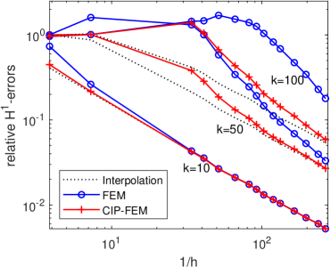
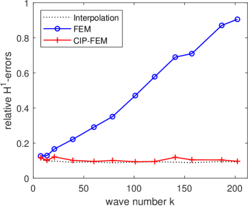
Fig. 5.1: The relative $H^{1}$-errors of the FE interpolation, the FE solution, and the CIP-FE solution.

5.2 Optical bistability

Optical bistability (see e.g. [4]) refers to the situation in which two different output intensities are possible for a given input intensity. It can be used as a switch in optical communication and in optical computing. We consider the NLH with $k=k_{0}=5.4$ in $\Omega_{0}^{c}$ and $k=k_{1}=3.5k_{0}$ in $\Omega_{0}$ (cf. [36, 37]). Set $h=10^{-2}$ and Kerr constant $\varepsilon=10^{-12}$, the incident wave $u_{\rm inc}=Ie^{{\rm\mathbf{i}}k_{0}x}$ and source term $f_{0}=0$, that is

$$f=\begin{cases}(k_{1}^{2}-k_{0}^{2})u_{\rm inc},&\text{in }\Omega_{0},\\ 0,&\text{otherwise}.\end{cases}$$

In this example, we set $\sigma_{0}=10$ and $L=1/4$ to reduce the computational area. Figure 5.2 plots the energy norm of the scattered field computed by the Newton’s method (4.33) versus that of the incident wave $u_{\rm inc}$. A reference incident wave $u_{\rm inc}^{0}=I_{0}e^{{\rm\mathbf{i}}k_{0}x}$ with $I_{0}=10^{5}$ is introduced for enhancing the nonlinear effect. Obviously, the larger the amplitude $I$, the stronger the intensity of the incident wave. The energy of the scattered field jumps to the upper branch from the lower branch as the intensity of the incident wave increases to $I\approx 264651$, and falls down from the upper branch to the lower branch as the intensity decreases to $I\approx 241294$. As shown in the figure, for $241294<I<264651$, the NLH has three different solutions, where the two solutions in the upper and lower branches are presumably stable, and the solution in the middle branch is unstable. This phenomenon corresponds to the optical bistability. For $I=255000$, the electric field patterns of these three solutions corresponding to the three circled points in Figure 5.2 are shown in Figure 5.3. As expected, the nonlinear phenomenon of optical bistability has been successfully simulated.

Finally, we compare the convergence rates of all the three methods (4.33)–(4.35) by solving the solution in the lower branch at $I=263000$ with the same initial values of zero. We use the solution computed by the Newton’s method (4.33) with a small tolerance $\mbox{tol}=10^{-13}$ (see (5.2)) as the “exact” CIP-FE solution $u_{h}$. The relative error and convergence order are defined by

$$e_{h}^{l}:=\frac{\left\|{\hskip-2.7pt}\left|u_{h}^{l}-u_{h}\right|{\hskip-2.7pt}\right\|}{\left\|{\hskip-2.7pt}\left|u_{h}\right|{\hskip-2.7pt}\right\|}\quad\mbox{and}\quad\mbox{order}:=\frac{\log e_{h}^{l+1}-\log e_{h}^{l}}{\log e_{h}^{l}-\log e_{h}^{l-1}},\quad l\geq 1.$$

The numerical results are listed in Table 5.1, which shows, as expected, that the Newton’s method converges quadratically while the other two methods converge linearly. There is no doubt, the Newton’s method converges much faster.

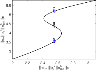
Fig. 5.2: X-axis: incident wave; Y-axis: scattered field. $I$ is $200000:310000$.

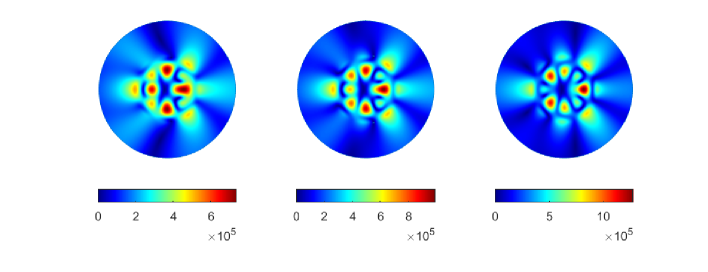
Fig. 5.3: Scattered field patterns of the three solutions marked as the points A, B, and C in Figure 5.2.

step		1	2	3	4	5	6	82	120
Newton	error	7.48e-2	2.85e-3	4.65e-3	1.40e-4	1.27e-7	9.36e-14
	order	-	0.37	1.88	1.93	2.00	2.02
modified Newton	error	4.11e-2	2.91e-2	2.05e-2	1.53e-2	1.12e-2	8.45e-3	9.10e-12
	order	-	0.11	1.01	0.84	1.07	0.91	1.00
frozen-nonlinearity	error	1.72e-1	1.19e-1	8.53e-2	6.34e-2	4.84e-2	3.76e-2	1.35e-8	9.22e-12
	order	-	0.21	0.90	0.89	0.91	0.93	1.00	1.00

Table 5.1: Relative errors and convergence orders of the iterative methods.

Appendix: A discrete stability estimate

Lemma A.1.

Given complex-valued functions $p,\,q\in L^{\infty}(\mathcal{D})$, and $\tilde{g}\in L^{2}(\mathcal{D})$, consider $\tilde{w}\in H_{0}^{1}(\mathcal{D})$ solving

(A.1) $$-\nabla\cdot(A\nabla\tilde{w})+p\tilde{w}+\overline{q\tilde{w}}=\tilde{g}$$

in the weak sense. Suppose there exists a positive constant $\tilde{c}_{0}$ such that the following stability estimate holds:

(A.2) $$\left\|\tilde{w}\right\|_{0}\leq\tilde{c}_{0}\left\|\tilde{g}\right\|_{0}.$$

Let $w_{h}\in V_{h}$ be the finite element solution to

(A.3) $$(A\nabla w_{h},\nabla v_{h})+(pw_{h},v_{h})+(q\overline{w_{h}},v_{h})=(g,v_{h})\quad\forall\,v_{h}\in V_{h}.$$

Then the FE solution satisfies the discrete stability estimates

(A.4) $$\left\|w_{h}\right\|_{0}\lesssim\tilde{c}_{0}\left\|g\right\|_{0}\quad\text{and}\quad\left\|\nabla w_{h}\right\|_{0}\lesssim\big{(}\left\|p\right\|_{L^{\infty}(\mathcal{D})}+\left\|q\right\|_{L^{\infty}(\mathcal{D})}+\tilde{c}_{0}^{-1}\big{)}^{\frac{1}{2}}\tilde{c}_{0}\left\|g\right\|_{0},$$

under the condition that the following quantity is sufficiently small:

(A.5) $$\big{(}1+(\left\|p\right\|_{L^{\infty}(\mathcal{D})}+\left\|q\right\|_{L^{\infty}(\mathcal{D})})\tilde{c}_{0}\big{)}\max\big{\{}\left\|p\right\|_{L^{\infty}(\mathcal{D})}+\left\|q\right\|_{L^{\infty}(\mathcal{D})},\tilde{c}_{0}^{-1}\big{\}}h^{2}\,.$$

Proof.

First, applying [21, Theorem 4.5] and using (A.2), we obtain the following regularity estimate:

$$\left\|\tilde{w}\right\|_{2,\Omega\cup\hat{\Omega}}\lesssim\left\|\tilde{g}-p\tilde{w}-\overline{q\tilde{w}}\right\|_{0}\lesssim\big{(}1+\big{(}\left\|p\right\|_{L^{\infty}(\mathcal{D})}+\left\|q\right\|_{L^{\infty}(\mathcal{D})}\big{)}\tilde{c}_{0}\big{)}\left\|\tilde{g}\right\|,$$

that is, there exists a positive constant $\tilde{c}_{2}\eqsim 1+\big{(}\left\|p\right\|_{L^{\infty}(\mathcal{D})}+\left\|q\right\|_{L^{\infty}(\mathcal{D})}\big{)}\tilde{c}_{0}$ such that

(A.6) $$\left\|\tilde{w}\right\|_{2,\Omega\cup\hat{\Omega}}\leq\tilde{c}_{2}\left\|\tilde{g}\right\|.$$

We use the convention $v=v_{r}+{\rm\mathbf{i}}v_{i}$ for all complex-valued functions, where $v_{r}$ and $v_{i}$ are both real-valued. Choosing $v_{h}:\mathcal{D}\to\mathbb{R}$ be any real function in (A.3) and taking the real and imaginary parts, we get

(A.7) $$(A_{r}\nabla w_{hr}-A_{i}\nabla w_{hi},\nabla v_{h})+(p_{r}w_{hr}-p_{i}w_{hi}+q_{r}w_{hr}+q_{i}w_{hi},v_{h}) =(g_{r},v_{h}),$$

(A.8) $$(A_{i}\nabla w_{hr}+A_{r}\nabla w_{hi},\nabla v_{h})+(p_{i}w_{hr}+p_{r}w_{hi}+q_{i}w_{hr}-q_{r}w_{hi},v_{h}) =(g_{i},v_{h}).$$

Let $z\in H_{0}^{1}(\mathcal{D})$ solve the dual problem $-\nabla\cdot(\overline{A}\nabla z)+\overline{p}z+q\overline{z}=w_{h}$ in $\mathcal{D}$, which can be rewritten as

(A.9) $$-\nabla\cdot(A_{r}\nabla z_{r})-\nabla\cdot(A_{i}\nabla z_{i})+(p_{r}z_{r}+p_{i}z_{i})+(q_{r}z_{r}+q_{i}z_{i}) =w_{hr},$$

(A.10) $$\nabla\cdot(A_{i}\nabla z_{r})-\nabla\cdot(A_{r}\nabla z_{i})+(p_{r}z_{i}-p_{i}z_{r})+(q_{i}z_{r}-q_{r}z_{i}) =w_{hi}.$$

Testing (A.9) and (A.10) by $w_{hr}$ and $w_{hi}$, respectively, and using (A.7)–(A.8) and the fact that $A$ is symmetric,

$$\left\|w_{h}\right\|_{0}^{2}= \;(A_{r}\nabla z_{r}+A_{i}\nabla z_{i},\nabla w_{hr})+(p_{r}z_{r}+p_{i}z_{i}+q_{r}z_{r}+q_{i}z_{i},w_{hr})$$

$$\;-(A_{i}\nabla z_{r}-A_{r}\nabla z_{i},\nabla w_{hi})+(p_{r}z_{i}-p_{i}z_{r}+q_{i}z_{r}-q_{r}z_{i},w_{hi})$$

$$= \;(A_{r}\nabla w_{hr}-A_{i}\nabla w_{hi},\nabla z_{r})+(p_{r}w_{hr}-p_{i}w_{hi}+q_{r}w_{hr}+q_{i}w_{hi},z_{r})$$

$$\;+(A_{i}\nabla w_{hr}+A_{r}\nabla w_{hi},\nabla z_{i})+(p_{i}w_{hr}+p_{r}w_{hi}+q_{i}w_{hr}-q_{r}w_{hi},z_{i})$$

$$= \;(A_{r}\nabla w_{hr}-A_{i}\nabla w_{hi},\nabla(z_{r}-(P_{h}z)_{r}))+(p_{r}w_{hr}-p_{i}w_{hi}+q_{r}w_{hr}+q_{i}w_{hi},z_{r}-(P_{h}z)_{r})$$

$$\;+(A_{i}\nabla w_{hr}+A_{r}\nabla w_{hi},\nabla(z_{i}-(P_{h}z)_{i}))+(p_{i}w_{hr}+p_{r}w_{hi}+q_{i}w_{hr}-q_{r}w_{hi},z_{i}-(P_{h}z)_{i})$$

$$\;+(g_{r},(P_{h}z)_{r}-z_{r})+(g_{r},z_{r})+(g_{i},(P_{h}z)_{i}-z_{i})+(g_{i},z_{i})$$

$$= \;(p_{r}w_{hr}-p_{i}w_{hi}+q_{r}w_{hr}+q_{i}w_{hi},z_{r}-(P_{h}z)_{r})+(p_{i}w_{hr}+p_{r}w_{hi}+q_{i}w_{hr}-q_{r}w_{hi},z_{i}-(P_{h}z)_{i})$$

$$\;+(g_{r},(P_{h}z)_{r}-z_{r})+(g_{r},z_{r})+(g_{i},(P_{h}z)_{i}-z_{i})+(g_{i},z_{i}),$$

where $P_{h}$ is the elliptic projection defined by (4.2) and we used $(A\nabla w_{h},\nabla(z-P_{h}z))=0$ to derive the last equality. Noting that $\overline{z}\in H_{0}^{1}(\mathcal{D})$ is the solution to (A.1) with $\tilde{g}=\overline{w_{h}}$, we deduce from (A.2) and (A.6) that

$$\left\|z\right\|_{0}\leq\tilde{c}_{0}\left\|w_{h}\right\|_{0}\quad\text{and}\quad\left\|z\right\|_{2,\Omega\cup\hat{\Omega}}\leq\tilde{c}_{2}\left\|w_{h}\right\|_{0}.$$

Therefore, the error estimate (4.3) yields

$$\left\|w_{h}\right\|_{0}^{2}\leq \;C_{\mathcal{E}}\tilde{c}_{2}h^{2}\big{(}(\left\|p\right\|_{L^{\infty}(\mathcal{D})}+\left\|q\right\|_{L^{\infty}(\mathcal{D})})\left\|w_{h}\right\|_{0}^{2}+\left\|g\right\|_{0}\left\|w_{h}\right\|_{0}\big{)}+\tilde{c}_{0}\left\|g\right\|_{0}\left\|w_{h}\right\|_{0},$$

where $C_{\mathcal{E}}$ is the invisible constant in (4.3). Letting

$$h_{0}^{2}=\min\big{\{}\big{(}2C_{\mathcal{E}}\tilde{c}_{2}(\left\|p\right\|_{L^{\infty}(\mathcal{D})}+\left\|q\right\|_{L^{\infty}(\mathcal{D})})\big{)}^{-1},(2C_{\mathcal{E}}\tilde{c}_{2})^{-1}\tilde{c}_{0}\big{\}},$$

we readily get the first estimate in (A.4) for $0<h\leq h_{0}$.

On the other hand, letting $v_{h}=w_{h}$ in (A.3) and using the derivations of (2.11)–(2.12) give

$$\left\|\nabla w_{h}\right\|_{0}^{2} \lesssim\Re(A\nabla w_{h},\nabla w_{h})\lesssim\big{(}\left\|p\right\|_{L^{\infty}(\mathcal{D})}+\left\|q\right\|_{L^{\infty}(\mathcal{D})}\big{)}\left\|w_{h}\right\|^{2}_{0}+\left\|g\right\|_{0}\left\|w_{h}\right\|_{0}$$

$$\lesssim\big{(}\left\|p\right\|_{L^{\infty}(\mathcal{D})}+\left\|q\right\|_{L^{\infty}(\mathcal{D})}+\tilde{c}_{0}^{-1}\big{)}\tilde{c}_{0}^{2}\left\|g\right\|_{0}^{2}.$$

Hence, (A.4) follows and the proof of this lemma is completed. ∎

References

- [1] I. Babuška and S. A. Sauter. Is the pollution effect of the FEM avoidable for the Helmholtz equation considering high wave numbers? SIAM Rev., 42(3):451–484, 2000.
- [2] G. Bao and H. Wu. Convergence analysis of the perfectly matched layer problems for time-harmonic Maxwell’s equations. SIAM J. Numer. Anal., 43(5):2121–2143, 2005.
- [3] J. P. Bérenger. A perfectly matched layer for the absorption of electromagnetic waves. J. Comput. Phys., 114(2):185–200, 1994.
- [4] R. Boyd. Nonlinear Optics. Academic, New York, 3rd edition, 2008.
- [5] J. H. Bramble and J. E. Pasciak. Analysis of a finite PML approximation for the three dimensional time-harmonic Maxwell and acoustic scattering problems. Math. Comp., 76(258):597–614, 2007.
- [6] S. C. Brenner and L. R. Scott. The Mathematical Theory of Finite Element Methods. Springer, 3rd edition, 2008.
- [7] T. Chaumont-Frelet, D. Gallistl, S. Nicaise, and J. Tomezyk. Wavenumber-explicit convergence analysis for finite element discretizations of time-harmonic wave propagation problems with perfectly matched layers. Commun. Math. Sci., 20(1):1–52, 2022.
- [8] Z. Chen and X. Liu. An adaptive perfectly matched layer technique for time-harmonic scattering problems. SIAM J. Numer. Anal., 43(2):645–671, 2005.
- [9] Z. Chen and H. Wu. An adaptive finite element method with perfectly matched absorbing layers for the wave scattering by periodic structures. SIAM J. Numer. Anal., 41(3):799–826, 2003.
- [10] W. Chew, J. Jin, and E. Michielssen. Complex coordinate stretching as a generalized absorbing boundary condition. Microw. Opt. Technol. Lett., 15(6):363–369, 1997.
- [11] P. G. Ciarlet. The Finite Element Method for Elliptic problems. North Holland, New York, 1978.
- [12] F. Collino and P. Monk. The Perfectly Matched Layer in Curvilinear Coordinates. SIAM J. Sci. Comput., 19(6):2061–2090, 1998.
- [13] J. Douglas and T. Dupont. Interior penalty procedures for elliptic and parabolic Galerkin methods. Lecture Notes in Phys., 58:207–216, 1976.
- [14] Y. Du and H. Wu. Preasymptotic error analysis of higher order FEM and CIP-FEM for Helmholtz equation with high wave number. SIAM J. Numer. Anal., 53(2):782–804, 2015.
- [15] L. C. Evans. Partial Differential Equations. Graduate Studies in Mathematics, 2nd edition, 2010.
- [16] X. Feng and H. Wu. Discontinuous Galerkin methods for the Helmholtz equation with large wave numbers. SIAM J. Numer. Anal., 47(4):2872–2896, 2009.
- [17] G. Fibich and B. Ilan. Vectorial and random effects in self-focusing and in multiple filamentation. Physica D, 157(1):112–146, 2001.
- [18] D. Gilbarg and N. S. Trudinger. Elliptic Partial Differential Equations of Second Order. Springer, Berlin, 2001.
- [19] C. J. Gittelson, R. Hiptmair, and I. Perugia. Plane wave discontinuous Galerkin methods: Analysis of the h-version. ESAIM Math. Model. Numer. Anal., 43(2):297–331, 2009.
- [20] C. Han. Dispersion analysis of the IPFEM for the Helmholtz equation with high wave number on equilateral triangular meshes. Master’s thesis, Nanjing University, 2012.
- [21] J. Huang and J. Zou. Uniform a priori estimates for elliptic and static Maxwell interface problems. Discrete Contin. Dyn. Syst.-Ser. B, 7(1):145, 2007.
- [22] F. Ihlenburg and I. Babuška. Finite element solution of the Helmholtz equation with high wave number. I. The -version of the FEM. Comput. Math. Appl., 30(9):9–37, 1995.
- [23] F. Ihlenburg and I. Babuška. Finite element solution of the Helmholtz equation with high wave number. II. The - version of the FEM. SIAM J. Numer. Anal., 34(1):315–358, 1997.
- [24] M. Lassas and E. Somersalo. On the existence and convergence of the solution of PML equations. Computing, 60(3):229–241, 1998.
- [25] M. Lenoir. Optimal isoparametric finite elements and error estimates for domains involving curved boundaries. SIAM J. Numer. Anal., 23(3):562–580, 1986.
- [26] Y. Li and H. Wu. FEM and CIP-FEM for Helmholtz equation with high wave number and perfectly matched layer truncation. SIAM J. Numer. Anal., 57(1):96–126, 2019.
- [27] W. C. H. McLean. Strongly elliptic systems and boundary integral equations. Cambridge University Press, 2000.
- [28] J. M. Melenk and S. A. Sauter. Convergence analysis for finite element discretizations of the Helmholtz equation with Dirichlet-to-Neumann boundary conditions. Math. Comp., 79(272):1871–1914, 2010.
- [29] J. M. Melenk and S.A. Sauter. Wavenumber explicit convergence analysis for Galerkin discretizations of the Helmholtz equation. SIAM J. Numer. Anal., 49(3):1210–1243, 2011.
- [30] J. C. Nédélec. Acoustic and electromagnetic equations. Springer, 2001.
- [31] L. Nirenberg. On Elliptic Partial Differential Equations. Ann. Scuola Norm. Sup. Pisa, 13(2):115–162, 1959.
- [32] F. W. J. Olver, D. W. Lozier, R. F. Boisvert, and C. W. Clark. NIST Handbook of Mathematical Functions. Cambridge University Press, New York, 2010 (see also http://dlmf.nist.gov).
- [33] A. H. Schatz and L. B. Wahlbin. Interior maximum norm estimates for finite element methods. Math. Comp., 31(138):414–442, 1977.
- [34] G. N. Watson. A Treatise on the Theory of Bessel Functions (Second Edition). Cambridge University Press, London, 1944.
- [35] H. Wu. Pre-asymptotic error analysis of CIP-FEM and FEM for the Helmholtz equation with high wave number. Part I: linear version. IMA J. Numer. Anal., 34(3):1266–1288, 2013.
- [36] H. Wu and J. Zou. Finite element method and its analysis for a nonlinear Helmholtz equation with high wave numbers. SIAM J. Numer. Anal., 56(3):1338–1359, 2018.
- [37] L. Yuan and Y. Lu. Robust iterative method for nonlinear Helmholtz equation. J. Comput. Phys., 343:1–9, 2017.
- [38] L. Zhu and H. Wu. Preasymptotic error analysis of CIP-FEM and FEM for Helmholtz equation with high wave number. Part II: -version. SIAM J. Numer. Anal., 51(3):1828–1852, 2013.