Deep Squared Euclidean Approximation to the Levenshtein Distance
for DNA Storage

Abstract

Storing information in DNA molecules is of great interest because of its advantages in longevity, high storage density, and low maintenance cost. A key step in the DNA storage pipeline is to efficiently cluster the retrieved DNA sequences according to their similarities. Levenshtein distance is the most suitable metric on the similarity between two DNA sequences, but it is inferior in terms of computational complexity and less compatible with mature clustering algorithms. In this work, we propose a novel deep squared Euclidean embedding for DNA sequences using Siamese neural network, squared Euclidean embedding, and chi-squared regression. The Levenshtein distance is approximated by the squared Euclidean distance between the embedding vectors, which is fast calculated and clustering algorithm friendly. The proposed approach is analyzed theoretically and experimentally. The results show that the proposed embedding is efficient and robust.

1 Introduction

With the increasing demand for storing information, scientists have been focusing on finding advanced storage media. DNA molecules, which carry most of the genetic information in vivo, have been tried as a new storage medium (Church et al., 2012; Goldman et al., 2013; Grass et al., 2015; Erlich & Zielinski, 2017; Organick et al., 2018; Dong et al., 2020; Chen et al., 2021). Studies have shown that the DNA storage has high storage density, low maintenance cost, and fast parallel replication (Ping et al., 2019; Dong et al., 2020).

A typical pipeline for storing information in synthetic DNA molecules includes the following steps (Dong et al., 2020). The binary data are firstly encoded as strings on the alphabet $\{\mathrm{A,C,G,T}\}$. Such strings are called references and usually have a fixed length in range $100-200$ nucleotides, which is limited by the biochemical techniques used to manipulate long DNA sequences. In the next step, the DNA molecules used as storage media are synthesized according to the references. These molecules are amplified and carefully preserved to increase the chances of future retrieval of the original information. To retrieve the stored information, the DNA molecules are sequenced into a bucket of strings, which are called the reads, on four bases $\{\mathrm{A,C,G,T}\}$. Due to the aforementioned amplification procedure, the set of reads usually includes several copies of each reference at the same time. Also, the biochemical procedures on DNA molecules are not fully reliable, hence the reads can contain errors such as base insertions, deletions or substitutions (Blawat et al., 2016). Finally, the references are recovered from the reads and decoded to retrieve the original binary data.

A straightforward way to recover references from the reads is to cluster the noisy reads by the Levenshtein distance (Levenshtein, 1966), and select one reference from each cluster. The Levenshtein distance between two strings, also known as the edit distance, is the minimum number of insertions, deletions, or substitutions required to modify one string to the other. Three issues arise when the size of stored information grows. First, the number of reads increases linearly with the amount of information stored, which leads to a squared increase in the computational complexity of a plain clustering algorithm (Rashtchian et al., 2017). Second, the Levenshtein distance is not easy to calculate. It is shown that the Levenshtein distance cannot be computed in $O(n^{2-\epsilon}),\forall\epsilon>0$, unless the strong exponential time hypothesis is false (Masek & Paterson, 1980; Backurs & Indyk, 2015). Third, most mature clustering algorithms are based on $\ell_{p}$ distance (Hartigan & Wong, 1979); these algorithms may fail or need to be adapted for Levenshtein distance. These three issues render the mission of clustering a large number of reads by plain algorithms impossible within reasonable time. Researchers have tried to address the challenge of clustering a huge amount of reads. For example, to cluster billions of the reads efficiently, Rashtchian et al. (Rashtchian et al., 2017) proposed a distributed, agglomerative clustering algorithm, based on the fact that clusters of the reads from a DNA storage pipeline are well-separated in Levenshtein distance. In their work, tools like the $q$-gram distance (Ukkonen, 1992) and locality sensitive hashing (LSH) (Har-Peled et al., 2012) were used for approximating the Levenshtein distance.

In this paper, the embedding of DNA sequences is investigated to approximate the Levenshtein distance. The basic idea is to map each DNA sequence to its embedding vector, and use the easy-calculated distance between the embedding vectors to approximate the Levenshtein distance between DNA sequences. With the embedding of DNA sequences, the task of clustering the huge number of reads in the DNA storage pipeline can be simplified by the following two aspects. First, the similarity between two DNA sequences can be computed more efficiently, because the computational complexity of the common distances, for example the $\ell_{p}$ distances, is $O(n)$, while the complexity of the Levenshtein distance is at least $O(n^{2-\epsilon})$. Second, numerous efficient clustering algorithms can be introduced into the DNA storage pipeline without much effort, as most of the mature clustering algorithms take $\ell_{p}$ distances as preferred distance measure.

Several existing works have attempted to map the Levenshtein distance to the easily calculated approximations (Hanada et al., 2017). In (Charikar & Krauthgamer, 2006; Ostrovsky & Rabani, 2007; Andoni et al., 2009), the Levenshtein distance on permutations or $\{0,1\}$-words was embedded into $\ell_{p}$ with low distortion. In (Chakraborty et al., 2016), the CGK-embedding was proposed, which is a randomized injective embedding of the Levenshtein distance into the Hamming distance; the application of this algorithm includes (Zhang & Zhang, 2017). The $q$-gram-based methods record the frequency distribution of the $q$-grams in strings and use it to approximate the Levenshtein distance, which include (Ukkonen, 1992; Bar-Yossef et al., 2004; Sokolov, 2007). Without the Levenshtein distance, more works on string similarity join have been proposed (Wang et al., 2014; Yu et al., 2016); most of these works are based on LSH, to name a few, (Buhler, 2001; Datar et al., 2004; Rasheed et al., ; Yuan et al., 2014).

Artificial neural networks (LeCun et al., 2015) were also utilized to provide sequence embeddings to compute approximations of the Levenshtein distance. Deep methods are often data-driven and have shown powerful feature extraction capabilities (LeCun et al., 2015). Therefore, it is assumed that deep learning-based approaches are more flexible and perform better in metric embedding on data with underlying structure or distribution. In (Zhang et al., 2020), the gated recurrent unit (GRU) (Cho et al., 2014), which is a famous variation of the recurrent neural network (RNN) (Rumelhart et al., 1985), was considered as a embedding function. The GRU was trained with a three-phased procedure and the triplet loss (Schroff et al., 2015) was engaged for similarity capturing. In (Dai et al., 2020), the researchers proved one-hot embedding and max-pooling preserve a bound on Levenshtein distance, and applied convolutional neural network (CNN) (Krizhevsky et al., 2012) for a convolutional embedding (CNN-ED). The authors also engaged the triplet loss to train their model. In (Corso et al., 2021), the authors reformulated existing approaches and explored related tasks, such as hierarchical clustering and multiple sequence alignment, with their NeuroSEED.

Considering that the exact Levenshtein distance costs at least $O(n^{2-\epsilon})$ in complexity, the following statement is straightforward.

Proposition 1.1.

If have no restrictions on the sequences, we can not find a deep learning-based sequence embedding that gives the Levenshtein distance by a conventional distance of complexity $O(n)$.

Although it is impossible to calculate the exact Levenshtein distance between arbitrary sequences by deep embedding, data-driven models can still be applied if the data show some “good” characteristics. In this paper, we use deep embedding to calculate the Levenshtein distance on a unique real-world dataset formed by the sequences from DNA storage experiments. The engaged dataset has specific underlying structures and distributions, from which we expect it to enable an efficient data-driven deep embedding. Features of the dataset are summarized as follows:

• The reads use fixed and finite alphabet $\{\mathrm{A,C,G,T}\}$ or $\{\mathrm{A,C,G,T,N}\}$, where the $\mathrm{N}$ represents failed bases in sequencing. Also, the length distribution of the reads is centered around the length of the references.

• The distributions of base insertions, deletions and substitutions are stable between two reads of the same cluster. In the study of (Blawat et al., 2016), it was shown that the error rates range from $0.1\%$ to $1\%$. In practice, two reads of about $150$ nucleotides from the same cluster have little chance of having a Levenshtein distance greater than $30$.

• The two reads from different clusters are completely unrelated to each other, which is ensured by the separated references from the DNA storage pipeline.

With regard to these features of the DNA sequences and the characteristics of deep embedding networks, we establish the deep squared Euclidean embedding (DSEE) method to approximate the Levenshtein distance by squared Euclidean distance on the dataset of DNA sequences. The proposed DSEE includes the following three main techniques.

• Instead of the triplet loss used in the related works (Dai et al., 2020; Zhang et al., 2020), the simple strategy of Siamese neural network (Bromley et al., 1993) is used to optimize the parameters of the embedding network. This simple setting helps us focus on the embedding of the Levenshtein distance.

• Instead of the $\ell_{p}$ distances, the squared Euclidean distance between the embedding vectors is used to approximate the Levenshtein distance between the original sequences. This enables us to mathematically interpret the Levenshtein distance from a completely new viewpoint. We establish the connection between the Levenshtein distance and the degree of freedom of the embeddings for the first time.

• Instead of regressions that uses mean squared error or mean absolute error as the optimization target, we propose the chi-squared regression, which uses a loss function that simulates the relative entropy from the chi-squared distribution. This loss function is skewed around the ground truth Levenshtein distance, and coincides with the theoretical distribution of the approximate distance in a more reasonable way.

With the squared Euclidean embedding and the chi-squared regression, our work reveals the critical part of a neural network-based embedding of Levenshtein distance for the first time. To the best of our knowledge, these techniques are introduced and analyzed both theoretically and experimentally for the first time in related fields.

The remainder of this paper is structured as follows. In Section 2, we provide some preliminaries on the focused embedding task. In Section 3, the proposed DSEE is introduced in detail. In Section 4, the experiments and ablation study are conducted. Some concluding remarks are presented in Section 5.

2 Notation, Dataset, and Metrics on Performance

2.1 Notations and Problem Statement

Given two reads $\bm{s},\bm{t}$ on the alphabet $\{\mathrm{A,C,G,T,N}\}$, where the $\mathrm{N}$ represents the bases that failed in sequencing, the Levenshtein distance $d_{L}(\bm{s},\bm{t})$ is the minimum number of insertions, deletions and substitutions required to convert $\bm{s}$ to $\bm{t}$. By its definition, the Levenshtein distance is symmetric on $\bm{s},\bm{t}$, i.e. $d_{L}(\bm{s},\bm{t})=d_{L}(\bm{t},\bm{s})$.

Let $\bm{u},\bm{v}$ be two vectors from the $n$-dimensional real space $\mathbb{R}^{n}$, the squared Euclidean distance is the square of the Euclidean distance ($\ell_{2}$ distance) between $\bm{u}$ and $\bm{v}$, which is

$$d_{\ell_{2}^{2}}=\sum_{i=1}^{n}(u_{i}-v_{i})^{2}.$$ (1)

It must be noticed that the triangle inequality does not hold for the squared Euclidean distance, hence the squared Euclidean distance does not form a metric space in mathematics. For convenience, we will still use the word “distance” for all the distance-like definitions, no matter they are real distances or not.

For a deep model that accepts only vectors, matrices, or tensors as its input data, we use the one-hot encoding to convert the DNA sequences into matrices. This was proved to be efficient in similar tasks (Dai et al., 2020). In the rest of this paper, the sequence $\bm{s}$ and its one-hot embedding $\mathrm{onehot}(\bm{s})$ will not be distinguished and the same notation $\bm{s}$ will be used.

As stated in the Section 1, the main task of this paper is to find a method to convert the reads into embedding vectors and to approximate the Levenshtein distance using the squared Euclidean distance between the embedding vectors. Mathematically, it can be interpreted as finding a function $f$ that maps the reads $\bm{s},\bm{t}$ to the embedding vectors $\bm{u}=f(\bm{s}),\bm{v}=f(\bm{t})$, such that the approximation error $|d_{L}(\bm{s},\bm{t})-d_{\ell_{2}^{2}}(\bm{u},\bm{v})|$ is small.

2.2 Dataset

The public data from the DNA-Fountain (Erlich & Zielinski, 2017), a well-known DNA storage study, is used for training and testing. It offers both the references and reads from their DNA storage pipeline. Each of the references has fixed length $152$ nucleotides, while the lengths of the reads are variable, for insertions or deletions of bases may occur in the biochemical procedure. In order to construct the training and testing sets, the DNA-Fountain data is divided into two parts according to a partition on the reference set. Each part of the data contains its selected references and the reads originate from those references. It is worth noting that the partition of the data keeps the training and testing sets disjoint.

Take the construction of the training set as an example. The training set is a collection of tuples $((\bm{s},\bm{t}),d)$, where the $(\bm{s},\bm{t})$ is a pair of DNA sequences and $d$ is the Levenshtein distance between them $d=d_{L}(\bm{s},\bm{t})$. Recall that the purpose of approximating Levenshtein distances is to cluster DNA sequences, the proposed embedding method should emphasize the separation of small and large distances. In view of this, the training set collects both homologous pairs and non-homologous pairs, where the sequences of homologous pair are generated from the same reference and have a small Levenshtein distance, while the sequences of non-homologous pair are completely independent and have a large Levenshtein distance. The ratio of homologous pairs to non-homologous pairs is set to $1:1$. Since a cluster of reads usually includes the identical copies of its source reference, the reference-read pairs are engaged as the homologous pairs in practice. For example, given a reference $\bm{r}^{i}$ and its reads $\{\bm{s}^{i}_{j}\}_{j}$, the homologous pairs are $\{(\bm{r}^{i},\bm{s}^{i}_{j})\}_{j}$ and the training set uses $((\bm{r}^{i},\bm{s}^{i}_{j}),d_{L}(\bm{r}^{i},\bm{s}^{i}_{j}))$ as its homologous samples. It is worth noting that, for any non-generative embedding method, the embedding vectors are the same for different runs on the same string. Therefore, pairs of identical sequences with Levenshtein distance $0$ are trival and should be screened out from the training set. As for the non-homologous pairs, a random selection of two reads $(\bm{s}^{i_{1}}_{j_{1}},\bm{s}^{i_{2}}_{j_{2}})$ from different references $\bm{r}^{i_{1}},\bm{r}^{i_{2}}\,(i_{1}\neq i_{2})$ will satisfy the requirement, and the training set uses the $((\bm{s}^{i_{1}}_{j_{1}},\bm{s}^{i_{2}}_{j_{2}}),d_{L}(\bm{s}^{i_{1}}_{j_{1}},\bm{s}^{i_{2}}_{j_{2}}))$ as its non-homologous samples. Finally, the training set is composed of samples $(\bm{s},\bm{t},d_{L}(\bm{s},\bm{t}))$ that include the homologous pairs and non-homologous pairs described above.

Considering the differences in the read lengths, all the sequences are padded with $0$ at the end to achieve a fixed length of $160$ nucleotides. In practice, homologous pairs with large distances occur at much lower rates than pairs with small distances, therefore, the samples are balanced by duplicating according to their Levenshtein distances.

2.3 Metrics on Performance

A common metric used in regression tasks is the approximation error ($\mathrm{AE}$). Given two sequences $\bm{s},\bm{t}$, let $\bm{u},\bm{v}$ be the two embedding vectors of these two sequences, respectively. In this paper, the mean absolute error (MAE) is engaged as the approximation error,

$$\mathrm{AE}=\mathrm{MAE}=\frac{1}{\#\mathrm{Te}}\sum_{(\bm{s},\bm{t})\in\mathrm{Te}}|d_{L}(\bm{s},\bm{t})-\hat{d}(\bm{u},\bm{v})|,$$ (2)

where the $\mathrm{Te}$ is for the testing set, and the $\hat{d}(u,v)$ is the approximate distance between embedding vectors $\bm{u},\bm{v}$.

In the specific task of this paper, the AE on the non-homologous pairs is less important than the AE on the homologous pairs. It is natural that the approximate distances are desired to be as accurate as possible on the homologous pairs. However, as stated in Proposition 1.1, a global accurate approximation is impossible. A careful dipiction on the Levenshtein distance between non-homologous sequences, which is the Levenshtein distance from random sequence to random sequence, is complex and meaningless. In view of this, a biased AE on the testing set is also considered to be an important metric on the performance of the method. Let $\mathrm{Te}_{h}$ be the collection of homologous pairs from the testing set $\mathrm{Te}$, the mean absolute error on $\mathrm{Te}_{h}$ ($\mathrm{MAE}_{h}$) is engaged as the biased approximation error ($\mathrm{AE}_{h}$),

$$\mathrm{AE}_{h}=\mathrm{MAE}_{h}=\frac{1}{\#\mathrm{Te}_{h}}\sum_{(\bm{s},\bm{t})\in\mathrm{Te}_{h}}|d_{L}(\bm{s},\bm{t})-\hat{d}(\bm{u},\bm{v})|,$$ (3)

where the $\mathrm{AE}_{h}$ only takes the homologous pairs into account.

One of the motivations of the proposed method is to use approximate distances to quickly determine whether two read have the same reference as a source. In the definition of the metric $\mathrm{AE}_{h}$, the approximation error on non-homologous pairs is dropped, but the proposed model should still have the ability to separate non-homologous and homologous pairs. To evaluate this ability, the metrics of classification tasks can be used. Given a threshold $K$, the testing samples can be divided into two groups by the approximate distance, which are

$$\hat{d}(\bm{u},\bm{v})\geq K$$ (4)

for the predicted non-homologous pairs and

$$\hat{d}(\bm{u},\bm{v})<K$$ (5)

for the predicted homologous pairs. Compare the predicted classification results with the ground truth partition of testing samples into homologous and non-homologous, the overall accuracy ($\mathrm{OA}$) from classification tasks is used to evaluate separation ability of the proposed methods.

3 Method

A typical deep model is a composite function of elementary neural network layers, which includes CNN, fully connected layer, etc.. It has been proved to be efficient in various tasks, including feature extraction and embedding (LeCun et al., 2015). In the proposed DSEE, the deep model is engaged as the embedding network to transform the DNA sequences into their embedding vectors. In detail, the embedding network is trained as a part of the Siamese neural network; the squared Euclidean distance is used as the embedding distance; and the model is trained by the chi-squared regression.

3.1 Siamese Neural Network

Siamese neural network is firstly introduced in (Bromley et al., 1993) for signature verification. It takes two inputs by two identical networks which share parameters, and gives the similarity on the inputs by comparing the outputs of the networks.

In DSEE, a Siamese structure is used for training the embedding model. Let $(\bm{s},\bm{t},d)$ be a sample from the training set, and $f(\cdot;\theta)$ be the embedding network, the Siamese neural network transforms the inputs by the procedure shown in Figure 1. The two DNA sequences $\bm{s},\bm{t}$ are firstly mapped to their respective embedding vectors ${\bm{u}}=f(\bm{s};\theta),{\bm{v}}=f(\bm{t};\theta)$ via two branches of the Siamese structure. Each branch of the Siamese network is fulfilled by a complete embedding network $f(\cdot;\theta)$; and the two branches of the embedding networks share the same weight $\theta$. Between the two embedding vectors ${\bm{u}},{\bm{v}}$, the approximate distance is calculated by $\hat{d}=d_{\ell_{2}^{2}}({\bm{u}},{\bm{v}})$, where $d_{\ell_{2}^{2}}(\cdot,\cdot)$ is the function of squared Euclidean distance, and the $\hat{d}$ is the approximation of the Levenshtein distance between the DNA sequences $\bm{s},\bm{t}$.

To learn a optimized $\hat{\theta}$, which enables the embedding network $f(\cdot;\hat{\theta})$, a cost or loss function $\mathcal{L}(\bm{d},\hat{\bm{d}};\theta)$ is defined by the ground truth Levenshtein distances $\bm{d}$ and the approxiamte distances $\bm{\hat{d}}$ on all the samples of the training set. With the loss function, finding optimized $\hat{\theta}$ can be mathematically interpreted as an optimization problem,

$$\hat{\theta}=\mathop{\arg\min}_{\theta}\mathcal{L}(\bm{d},\hat{\bm{d}};\theta).$$ (6)

Gradient-based optimization methods are usually used to find a local minima of $\mathcal{L}(\bm{d},\hat{\bm{d}};\theta)$. Variations of gradient-based methods include the stochastic gradient descent (SGD) (Robbins & Monro, 1951) optimizer, Adam optimizer (Kingma & Ba, 2015), etc..

Figure 1: Siamese neural network. The two DNA sequences $\bm{s},\bm{t}$ are mapped to respective embedding vectors $\bm{u},\bm{v}$ via two branches which share the same parameters. The approximate distance is calculated by the squared Euclidean distance between $\bm{u}$ and $\bm{v}$.

3.2 Embedding Space and Chi-Squared Regression

As mentioned above, the Levenshtein distance has been approximated by the $\ell_{1}$ distance, the Euclidean distance ($\ell_{2}$ distance), the Hamming distance, etc. (Charikar & Krauthgamer, 2006; Ostrovsky & Rabani, 2007; Andoni et al., 2009; Chakraborty et al., 2016; Zhang & Zhang, 2017). In this paper, to ensure that gradient-based optimization is applicable, the differentiable distances, i.e. the $\ell_{1}$ distance and $\ell_{2}$ distance, are considered as alternative approximations of the Levenshtein distance. While in the proposed DSEE, the squared Euclidean distance is applied as the approximation of Levenshtein distance. Although the squared Euclidean distance does not form a metric space, we still find it experimentally and theoretically superior to the $\ell_{1}$ and $\ell_{2}$ distances (see Section 4, Appendix C and Appendix D).

Let’s make some assumptions or restrictions before further analysis. First, given a sequence $\bm{s}$, we assume that each element $u_{i}$ of the embedding vector $\bm{u}=f(\bm{s})$ follows a standard normal distribution $N(0,1)$. If the embedding network $f(\cdot)$ uses a batch normalization layer before its output, the mean value and standard deviation of $u_{i}$ are approximately equal to $0$ and $1$ respectively. As the normal distribution is the most common type, we expect the distribution of $u_{i}$ to be close to normal in practice. Second, if we have trained a good embedding network $f(\cdot)$, the elements $u_{i}$ and $u_{j}$ are expected to be independent of each other if $i\neq j$. This is partly because that the independent embedding elements can hold more information about the original sequence. Third, given another sequence $\bm{t}$ that is non-homologous to the sequence $\bm{s}$, the embedding vector $\bm{v}=f(\bm{t})$ is independent to the embedding vector $\bm{u}$ of sequence $\bm{s}$. In addition, the expected distance between the independent embedding vectors $\bm{u}$ and $\bm{v}$ should meet the mean value of the Levenshtein distance between two non-homologous sequences. To verify whether these assumptions hold in practice, we analyze the distributions and independence of the embedding elements in Appendix D. The results show that the normality assumption is maintained in practice, and that the proposed method helps to improve the independence between the embedding elements.

The average Levenshtein distance between two non-homologous sequences on the DNA-Fountain data is about $80$, and we use this number $n=80$ as the dimension of the embedding vectors. This setting implies that each position of the two independent embedding vectors contributes $1$ to the approximate distance. In addition, we also believe that $n=80$ is not too large to cost too much computational complexity, nor too small to degrade the performance of the method. In order to satisfy the third restriction mentioned above, we need to rescale the embedding vector before computing the approximate distance. The rescaling factor for squared Euclidean distance is

$$r_{\ell_{2}^{2}}=\frac{\sqrt{2}}{2}.$$ (7)

For convenience, from now on, the symbols $\bm{u},\bm{v}$ are used to denote the scaled embedding vectors, for example,

$$\bm{u}=r_{\ell_{2}^{2}}f(\bm{s})=\frac{\sqrt{2}}{2}f(\bm{s}).$$ (8)

By rescaling, the vector elements $u_{i}$,$v_{i}$ follow the distribution $N(0,1/2)$, hence the $u_{i}-v_{i}$ follows the standard normal distribution $N(0,1)$ when $\bm{u}$ and $\bm{v}$ are independent. Recall that the squared Euclidean distance is defined as

$$d_{\ell_{2}^{2}}(\bm{u},\bm{v})=\sum_{i=1}^{n}(u_{i}-v_{i})^{2}.$$ (9)

The squared Euclidean distance between two independent embedding vectors follows the chi-squared distribution $\chi^{2}(n)$ with the embedding dimension $n$ as the degree of freedom. As mentioned above, the embedding dimension $n$ is set to $n=80$ to equal the average Levenshtein distance of two non-homologous sequences. The expected distance between two independent embedding vectors is

$$E(d_{\ell_{2}^{2}}(\bm{u},\bm{v}))=80,\quad d_{\ell_{2}^{2}}(\bm{u},\bm{v})\sim\chi^{2}(80),$$ (10)

which coincides with the average Levenshtein distance between two non-homologous sequences.

To train deep models for approximation, existing works used the mean squared error, the mean absolute error, or their variations as the loss functions on the approximate distance $\hat{d}$ and the Levenshtein distance $d$. In the gradient descent algorithms, these loss functions and their gradients with respect to the predicted distance $\hat{d}$ are symmetric about the ground truth distance $d$. For example, the mean squared error on $\hat{d}$ and $d$ is

$$\mathrm{MSE}(\hat{d},d)=(\hat{d}-d)^{2},$$ (11)

and the partial derivative with respect to $\hat{d}$ is $2(\hat{d}-d)$, which are symmetric about $d$. However, the distributions of predicted distance $\hat{d}$, the ground truth distance $d$, and especially the difference between these two distances $\hat{d}-d$ are skewed rather than symmetric. The skewed distributions are more pronounced when the ground truth distance is small. For example, a predicted distance $\hat{d}=2.5$ with positive deviation of $1.5$ on ground truth distance $d=1$ is reasonable, but in no case should the method predict a distance as $\hat{d}=-0.5$ with negative deviation $-1.5$ on the same ground truth distance.

To tackle this issue, we introduce the chi-squared regression for training the embedding network. Instead of optimizing an approximate error between predicted distance $\hat{d}$ and ground truth distance $d$, the chi-squared regression interprets the Levensthein distance $d$ as the degree of freedom of $\bm{u}-\bm{v}$ and uses a loss function that simulates the relative entropy (also called Kullback–Leibler divergence (Kullback & Leibler, 1951)) to chi-squared distribution $\chi^{2}(d)$.

Recall that the squared Euclidean distance between two independent embedding vectors follows the $\chi^{2}(n)$ distribution with the degree of freedom equal to the embedding dimension. For two dependent embedding vectors, the chi-squared distribution is also applicable for the distribution of the squared Euclidean distance by the following steps. In this paper, we call a multivariable $\bm{x}=(x_{1},\ldots,x_{n})$ to have a degree of freedom $d$, iff there exists an orthogonal matrix $\bm{P}$ and a multivariable $\bm{y}$ such that

$$\bm{x}=\bm{y}\bm{P}=(y_{1},\ldots,y_{d},0,\ldots,0)\bm{P},$$ (12)

where the $y_{i}$s are i.i.d. and follow $N(0,1)$. If the difference between two embedding vectors $\bm{u},\bm{v}$ has a degree of freedom $d$, which is

$$\bm{u}-\bm{v}=\bm{y}\bm{P}=(y_{1},\ldots,y_{d},0,\ldots,0)\bm{P},$$ (13)

the squared Euclidean distance between them is calculated as

$$d_{\ell_{2}^{2}}(\bm{u},\bm{v}) =\sum_{i=1}^{n}(u_{i}-v_{i})^{2}=(\bm{u}-\bm{v})(\bm{u}-\bm{v})^{T}$$

$$=\bm{y}\bm{P}\bm{P}^{T}\bm{y}^{T}=\bm{y}\bm{y}^{T}$$

$$=\sum_{i=1}^{d}y_{i}^{2},$$ (14)

and follows the chi-squared distribution $\chi^{2}(d)$ with degree of freedom $d$. A step further, the expected value of the squared Eulidean distance between $\bm{u}$ and $\bm{v}$ is the degree of freedom $d$ of their difference $\bm{u}-\bm{v}$. In view of this, it is a reasonable idea to make connections from the Levenshtein distance between the sequences $\bm{s},\bm{t}$ to the degree of freedom of the difference $\bm{u}-\bm{v}$ between their embedding vectors. The smaller the Levenshtein distance between the sequences $\bm{s}$ and $\bm{t}$ is, the more related their embedding vectors $\bm{u}$ and $\bm{v}$ are, and the less free variables $y_{i}$s are needed to support the difference $\bm{u}-\bm{v}$. To be precise, if the Levenshtein distance between two sequences $\bm{s}$ and $\bm{t}$ is $d$, we expect that the difference $\bm{u}-\bm{v}$ between their embedding vectors has a degree of freedom $d$. By this, the squared Euclidean distance $d_{\ell_{2}^{2}}(\bm{u},\bm{v})$ follows the $\chi^{2}(d)$ and its expected value equals the degree of freedom and equals the Levenshtein distance between $\bm{s}$ and $\bm{t}$.

In order to define the loss function between predicted distance $\hat{d}$ to the distribution $\chi^{2}(d)$, the relative entropy is used. Mathematically, the relative entropy of distrubtion $P$ from $Q$ is defined as

$$\mathrm{KLD}(P||Q)=\int_{-\infty}^{\infty}p(x)\log\frac{p(x)}{q(x)}\mathrm{d}x.$$ (15)

Let $P$ be the distribution of the predicted distance $\hat{d}$ and $Q_{d}=\chi^{2}(d)$ be the chi squared distribution with degree of freedom $d$,

$$\mathrm{KLD}(P||Q_{d})=\mathbb{E}_{\hat{d}\sim P}[\log p(\hat{d})]-\mathbb{E}_{\hat{d}\sim P}[\log q_{d}(\hat{d})].$$ (16)

For the first term of Equation 16 is not accessable, we use the second term as the optimization target, which is

$$\mathrm{RE}\chi^{2}(\hat{d},d) =-\log{q_{d}(\hat{d})}$$

$$=\frac{d}{2}+\log\Gamma\left(\frac{d}{2}\right)-\left(\frac{d}{2}-1\right)\log\hat{d}$$

$$+\frac{\hat{d}}{2}\log\mathrm{e},$$ (17)

where the $\Gamma$ is the Gamma function,the $\mathrm{e}$ is the Euler’s number, and the $\log$ uses $2$ as the base. It is worthy to note that the Section 3.2 can also be interpreted as the cross-entropy between the distribution of $\hat{d}$ and the chi squared distribution, or a loss of negative log-likelihood.

In summary, the proposed DSEE mainly consists of the following parts: a deep model $f(\cdot;\theta)$ for mapping the sequences to their embedding vectors; a Siamese network for calculating the approximations of the Levenshtein distance by the squared Euclidean distance; and the RE$\chi^{2}$ loss function for penalizing the difference between the approximate and the ground truth distances. In the training phase, the parameters $\theta$ are optimized to $\hat{\theta}$ subject to minimizing the relative entropy loss RE$\chi^{2}$, while in the testing phase, the trained deep model $f(\cdot;\hat{\theta})$ is used to output the embedding vectors of sequences, and the squared Euclidean distance between the embedding vectors are used as the approximations of the Levenshtein distance.

4 Experiments and Analysis

The proposed method includes the following variables: the embedding network $f(\cdot;\theta)$; the embedding space of the Levenshtein distance; and the loss function to be optimized. To find suitable network structures for the embedding network $f(\cdot;\theta)$, several mainstream structures, the CNN-ED-5, the CNN-ED-10, the RNN, and the GRU, are applied in the experiments. To show the advantages of the proposed squared Euclidean embedding, the experiments on the $\ell_{1}$ embedding and the $\ell_{2}$ embedding of the Levenshtein distance are conducted. Finally, to illustrate the advantages of the proposed chi-square regression, we conduct comparative experiments using the mean squared error and mean absolute error as loss functions.

To obtain a comprehensive view on how these three variables interact with each other and affect the performance of the proposed method, all combinations of these experimental setups are explored. The results are reported in Table 1. In this table, the column headers indicate the engaged structures of the embedding network and the loss functions used in the training phase, for example, the “CNN-ED-5: RE$\chi^{2}$” means the CNN-ED-5 structure and the RE$\chi^{2}$ loss. The row headers indicate the metrics used to evaluate the testing performance of the methods and the embedding spaces of the features, for example, the “$\mathrm{AE}_{h}$: $\ell_{2}$” means the $\mathrm{AE}_{h}$ metric predifined in Section 2.3 and the $\ell_{2}$ embedding of the sequences. The results in Table 1 are reported in the format “$\mathrm{mean}\pm\mathrm{std}$” of the mean value and the standard deviation over $5$ runs of the experiments. It is worth noting that the RE$\chi^{2}$ loss is incompatible with the $\ell_{1}$ and $\ell_{2}$ embeddings of the sequences, and we make the relevant numbers italicized in Table 1. We have also marked the “good” results in boldface, which are the $\mathrm{AE}_{h}$ less than $1.00$ and the $\mathrm{OA}$ greater than $99.90\%$.

Table 1: Results of the experiments. The column headers indicate the engaged structures of the embedding network and the loss functions used in the training phase, while the row headers indicate the metrics used to evaluate the testing performance and the embedding spaces of the features. The results are reported in the format “$\mathrm{mean}\pm\mathrm{std}$” of the mean value and the standard deviation over $5$ runs of the experiments. The italicized numbers are the results obtained by applying RE$\chi^{2}$ loss on the $\ell_{1}$ and $\ell_{2}$ embeddings, where the RE$\chi^{2}$ loss is incompatible with this embedding spaces. The boldface numbers are the “good” results of $\mathrm{AE}_{h}$ less than $1.00$ and the $\mathrm{OA}$ greater than $99.90\%$.

Metric	Embed	CNN-ED-5			CNN-ED-10
		MSE	MAE	RE$\chi^{2}$	MSE	MAE	RE$\chi^{2}$
	$\ell_{1}$	4.74 $\pm$ 0.03	3.57 $\pm$ 0.18	5.66 $\pm$ 0.15	4.60 $\pm$ 0.13	3.70 $\pm$ 0.16	5.26 $\pm$ 0.04
	$\ell_{2}$	6.23 $\pm$ 0.01	3.73 $\pm$ 0.11	6.02 $\pm$ 0.42	5.93 $\pm$ 0.07	3.56 $\pm$ 0.06	5.00 $\pm$ 0.06
$\mathrm{AE}$	$\ell_{2}^{2}$	4.20 $\pm$ 0.06	4.12 $\pm$ 0.02	4.67 $\pm$ 0.09	4.11 $\pm$ 0.01	4.12 $\pm$ 0.08	4.53 $\pm$ 0.03
	$\ell_{1}$	3.50 $\pm$ 0.02	2.50 $\pm$ 0.15	1.89 $\pm$ 0.05	3.44 $\pm$ 0.04	2.71 $\pm$ 0.19	1.96 $\pm$ 0.01
	$\ell_{2}$	5.99 $\pm$ 0.01	2.69 $\pm$ 0.08	2.59 $\pm$ 0.03	5.88 $\pm$ 0.02	2.69 $\pm$ 0.14	2.77 $\pm$ 0.05
$\mathrm{AE}_{h}$	$\ell_{2}^{2}$	0.90 $\pm$ 0.05	0.96 $\pm$ 0.09	0.90 $\pm$ 0.00	1.11 $\pm$ 0.02	1.56 $\pm$ 0.15	0.91 $\pm$ 0.01
	$\ell_{1}$	99.98 $\pm$ 0.00	96.57 $\pm$ 0.30	99.42 $\pm$ 0.11	99.98 $\pm$ 0.01	96.59 $\pm$ 0.27	99.27 $\pm$ 0.04
	$\ell_{2}$	99.85 $\pm$ 0.01	96.40 $\pm$ 0.26	98.34 $\pm$ 0.09	99.66 $\pm$ 0.06	96.81 $\pm$ 0.09	98.14 $\pm$ 0.02
$\mathrm{OA}$	$\ell_{2}^{2}$	99.98 $\pm$ 0.01	99.85 $\pm$ 0.08	99.98 $\pm$ 0.00	99.91 $\pm$ 0.00	99.06 $\pm$ 0.16	99.98 $\pm$ 0.01

Metric	Embed	RNN			GRU
		MSE	MAE	RE$\chi^{2}$	MSE	MAE	RE$\chi^{2}$
	$\ell_{1}$	5.25 $\pm$ 0.05	4.32 $\pm$ 0.43	5.89 $\pm$ 0.18	4.61 $\pm$ 0.14	3.45 $\pm$ 0.26	5.36 $\pm$ 0.06
	$\ell_{2}$	7.15 $\pm$ 0.08	5.11 $\pm$ 0.44	6.71 $\pm$ 0.33	7.52 $\pm$ 0.15	3.89 $\pm$ 0.15	5.32 $\pm$ 0.05
$\mathrm{AE}$	$\ell_{2}^{2}$	4.31 $\pm$ 0.01	4.36 $\pm$ 0.06	5.41 $\pm$ 0.02	3.98 $\pm$ 0.02	4.05 $\pm$ 0.02	5.51 $\pm$ 0.05
	$\ell_{1}$	4.06 $\pm$ 0.05	3.25 $\pm$ 0.28	2.25 $\pm$ 0.03	3.55 $\pm$ 0.09	2.48 $\pm$ 0.27	2.09 $\pm$ 0.05
	$\ell_{2}$	6.49 $\pm$ 0.15	3.56 $\pm$ 0.26	3.15 $\pm$ 0.14	6.40 $\pm$ 0.04	2.75 $\pm$ 0.09	2.73 $\pm$ 0.02
$\mathrm{AE}_{h}$	$\ell_{2}^{2}$	1.03 $\pm$ 0.02	1.14 $\pm$ 0.24	0.91 $\pm$ 0.01	0.73 $\pm$ 0.03	0.67 $\pm$ 0.02	0.88 $\pm$ 0.00
	$\ell_{1}$	99.96 $\pm$ 0.01	96.51 $\pm$ 0.42	99.15 $\pm$ 0.13	99.98 $\pm$ 0.00	96.72 $\pm$ 0.25	99.40 $\pm$ 0.14
	$\ell_{2}$	99.77 $\pm$ 0.02	96.10 $\pm$ 0.87	98.23 $\pm$ 0.13	99.88 $\pm$ 0.01	96.25 $\pm$ 0.26	98.21 $\pm$ 0.02
$\mathrm{OA}$	$\ell_{2}^{2}$	99.96 $\pm$ 0.00	99.77 $\pm$ 0.18	99.94 $\pm$ 0.00	100.00$\pm$ 0.00	99.99 $\pm$ 0.00	99.97 $\pm$ 0.00

As stated in Section 2.3, the metric $\mathrm{AE}$ presents the global approximation error for all the homologous and non-homologous sequence pairs. A small $\mathrm{AE}$ indicates that the model is well trained and performs well. However, a precise approximation of the Levenshtein distance for non-homologous pair is less of our interest, hence under the premise that $\mathrm{AE}$ is small, the $\mathrm{AE}_{h}$ is a more important metric to evaluate the testing performance of the models. As illustrated in Table 1, all the experiments show small $\mathrm{AE}$, in view of this, the $\mathrm{AE}_{h}$ and the $\mathrm{OA}$ will be discussed mainly in further analysis.

The squared Euclidean embedding takes the lead by a large margin. Let us fix the structure of embedding network and loss function, and compare the embedding spaces. The squared Euclidean embedding is several times superior to the $\ell_{1}$ embedding in metric $\mathrm{AE}_{h}$ over all the combinations of embedding networks and loss functions. $\mathrm{OA}$ of squared Euclidean embedding is also higher than $\mathrm{OA}$ of $\ell_{1}$ embedding in most cases. Meanwhile, the $\ell_{2}$ embedding performs the worst among three embedding spaces. Briefly, the three embeddings are ranked as $\ell_{2}^{2}>\ell_{1}>\ell_{2}$. We provide a preliminary analysis of these results in Appendix C.

The proposed chi-squared regression also shows good performance. When the squared Euclidean embedding is used, applying the RE$\chi^{2}$ loss improves the performance of the networks CNN-ED-10 and RNN in metrics $\mathrm{AE}_{h}$ and $\mathrm{OA}$ by a large margin, while on the networks CNN-ED-5 and GRU, the RE$\chi^{2}$ loss also has comparable performance to MAE and MSE losses. As mentioned above, the RE$\chi^{2}$ loss is incompatible with the $\ell_{1}$ and $\ell_{2}$ embeddings under the assumptions in Section 3.2. However, brutely applying the RE$\chi^{2}$ loss on the $\ell_{1}$ and $\ell_{2}$ embeddings still shows performance better than or equal to the MSE and MAE losses. We conjecture that the powerful fitting ability of neural networks overcomes the inability of the $\ell_{1}$ and $\ell_{2}$ embeddings to conduct the chi-squared distribution $\chi^{2}(d)$.

As illustrated in Table 1, different choices of the embedding network $f(\cdot;\theta)$ have similar performance for most combinations of embedding spaces and loss functions. The only exception occurs on squared Euclidean embedding, to be precise, GRU outperforms the other three embedding networks in metric $\mathrm{AE}_{h}$, no matter which loss function is engaged. Because GRU is the most modern and complex one among four models, it was believed to have better performance globally. However, experiments have shown that only the squared Euclidean embedding enables the GRU. We may infer that the application of the squared Euclidean embedding not only helps to improve the performance, but also helps to discover the potential of complex embedding networks. It is also worth noting that, no matter which model is used, the combination of squared Euclidean embedding and the RE$\chi^{2}$ loss always has a stable and excellent performance.

We leave the details of the experiments to the Appendices, including the rescaling factors for the $\ell_{1}$ and $\ell_{2}$ embeddings Appendix A and the setups for applied embedding networks Appendix B.

5 Conclusion

Fast approximation of the Levenshtein distance is demanded by a lot applications. In this paper, raised from DNA storage researches, the deep squared Euclidean embedding (DSEE) of DNA sequences was proposed to approximate the Levenshtein distance. The proposed method consists of three main components, namely, the Siamese neural network, the squared Euclidean embedding, and the chi-squared regression. It is innovative in applying the squared Euclidean embedding to approximate the Levenshtein distance, interpreting the Levenshtein distance between the sequences as the degree of freedom of their embeddings, and introducing the relative entropy to $\chi^{2}$ distribution as the loss function. The advantages of the proposed DSEE were theoretically analyzed under concise and reasonable assumptions. We also conducted comprehensive experiments and ablation studies. The experimental results echoed the theoretical analysis and showed that the proposed DSEE is powerful in approximating the Levenshtein distance.

Appendix A Rescaling factors for $\ell_{1}$ and $\ell_{2}$ embeddings

The $\ell_{1}$ and $\ell_{2}$ distances between the embedding vectors are considered as alternative approximations of the Levenshtein distance between the original sequences. To satisfy the restriction that the approximate distance between two independent embedding vectors should equal to the average Levenshtein distance between two non-homologous sequences, the $\ell_{1}$ and $\ell_{2}$ embeddings also need to be rescaled.

The rescaling factor for $\ell_{1}$ embedding vectors is

$$r_{\ell_{1}}=\frac{\sqrt{\pi}}{2}.$$ (18)

Given two independent embedding vectors $\bm{u}$ and $\bm{v}$, the $\ell_{1}$ distance between them is

$$d_{\ell_{1}}(\bm{u},\bm{v})=\sum_{i=1}^{n}|u_{i}-v_{i}|.$$ (19)

By rescaling, each element of the vectors $\bm{u}$ and $\bm{v}$ follows the normal distribution $N(0,\pi/4)$ independently. Therefore, the $|u_{i}-v_{i}|$ in Equation 19 follows the half-normal distribution $HN(\sqrt{\pi/2})$, and the expected value of $|u_{i}-v_{i}|$ is $E(|u_{i}-v_{i}|)=1$. The expected value of $d_{\ell_{1}}(\bm{u},\bm{v})$ in Equation 19 is easily computed as the dimension of the embedding vector

$$E(d_{\ell_{1}}(\bm{u},\bm{v}))=n=80,$$ (20)

which is also the average Levenshtein distance between two non-homologous sequences. It is worth noting that the distribution of $d_{\ell_{1}}(\bm{u},\bm{v})$ is not easy to depict, and the relative entropy to these family of distributions is difficult to calculate.

The rescaling factor for $\ell_{2}$ embedding vectors is

$$r_{\ell_{2}}=\frac{n\Gamma(n/2)}{2\Gamma((n+1)/2)}.$$ (21)

The $\ell_{2}$ distance between two independent embedding vectors $\bm{u}$ and $\bm{v}$ is calculated by

$$d_{\ell_{2}}(\bm{u},\bm{v})=\left(\sum_{i=1}^{n}(u_{i}-v_{i})^{2}\right)^{\frac{1}{2}}.$$ (22)

In view of the independence of the vector elements of $\bm{u}$ and $\bm{v}$, the $u_{i}-v_{i}$ follows the normal distribution, which is

$$\frac{u_{i}-v_{i}}{\sqrt{2}r_{\ell_{2}}}\sim N(0,1).$$ (23)

Hence, the rescaled $\ell_{2}$ distance between $\bm{u}$ and $\bm{v}$

$$\frac{d_{\ell_{2}}(\bm{u},\bm{v})}{\sqrt{2}r_{\ell_{2}}}=\left(\sum_{i=1}^{n}\left(\frac{u_{i}-v_{i}}{\sqrt{2}r_{\ell_{2}}}\right)^{2}\right)^{\frac{1}{2}},$$ (24)

follows the chi distribution $\chi(n)$ with degree $n$ of freedom. By the formula of expected value of chi distribution, the expected value of the $\ell_{2}$ distance is

$$E(d_{\ell_{2}}(\bm{u},\bm{v})) =\sqrt{2}r_{\ell_{2}}E\left(\frac{d_{\ell_{2}}(\bm{u},\bm{v})}{\sqrt{2}r_{\ell_{2}}}\right)$$

$$=\sqrt{2}\frac{n\Gamma(n/2)}{2\Gamma((n+1/2))}\cdot\sqrt{2}\frac{\Gamma((n+1)/2)}{\Gamma(n/2)}$$

$$=n,$$ (25)

where the $n=80$ is the preset dimension of the embedding vector and the average Levenshtein distance between two non-homologous sequences. Similar to the $\ell_{1}$ embedding, the $\ell_{2}$ embedding is also incompatible with the relative entropy. Given a chi distribution $\chi(k)$, the expected value is

$$E(x)=\sqrt{2}\frac{\Gamma((k+1)/2)}{\Gamma(k/2)},\quad x\sim\chi(k),$$ (26)

which does not equal the parameter $k$ of the chi distribution. If we apply the ground truth Levenshtein distance $d$ as the degree of freedom of the chi distribution and force the predicted $\ell_{2}$ distance $\hat{d}$ to obey $\chi(d)$, the expected value of $\hat{d}$ does not equal to the ground truth $d$. In view of this, the relative entropy to chi distribution is defined meaningless.

Appendix B Details on the embedding networks

In the experiments, four structures of the embedding networks are used, namely the CNN-ED-5, the CNN-ED-10, the RNN, and the GRU.

The CNN-ED-5 and CNN-ED-10 were proposed in (Dai et al., 2020). These two CNNs have similar structure by stacking layers of CNNs, activations, and average poolings. Taking the CNN-ED-5 as an example, the model stacks the following layers in five times, which are the $1$D-CNN (output channels: $64$, kernel size: $3$, stride: $1$, and padding size: $1$), the average pooling (kernel size: $2$), and the activation of ReLU. After these CNNs, two cascaded fully connected layers transform the features into a dimension of $n=80$, and a batch normalization is engaged to force the output to follow the $N(0,1)$. The CNN-ED-10 doubles the $1$D-CNN layers in CNN-ED-5, while the other parts of the structure remain the same. The model RNN is a stacked RNN of two recurrent units and bidirectional. The size of its hidden features is $64$ and the activation is $\mathrm{tanh}$. After the recurrent units, the model of RNN uses the same top of the fully connected layers and batch normalization with CNN-ED-X. The model GRU totally follows the same structure of model RNN, but it uses the GRU as the recurrent units. The parameters of its recurrent units are also the same with the model RNN.

Appendix C Why $\ell_{2}^{2}>\ell_{1}>\ell_{2}$?

The chi-squared regression is based on the straightforward assumption that the degree of freedom of the difference between the embedding vectors is consistent with the Levenshtein distance. To be precise, let $\bm{s},\bm{t}$ be two random sequences with Levenshtein distance $d$, and $\bm{u},\bm{v}$ be their respective embedding vectors, there exists an orthogonal matrix $\bm{P}$ such that

$$\bm{u}-\bm{v} =\bm{y}\bm{P}$$

$$=(y_{1},y_{2},\ldots,y_{d},0,\ldots,0)\bm{P},$$ (27)

where the $y_{i}$ are random variables that follow the standard normal distribution $N(0,1)$ independently, and the $d$ is the Levenshtein distance $d_{L}(\bm{s},\bm{t})$ between $\bm{s}$ and $\bm{t}$.

Under this assumption, we demonstrate that the expected value of $\ell_{2}^{2}$ distance between two embedding vectors $\bm{u},\bm{v}$ matches the degree of freedom $d$ of $\bm{u}-\bm{v}$, which is also the Levenshtein distance $d$ between sequences $\bm{s}$ and $\bm{t}$. But the expected values of $\ell_{1}$ and $\ell_{2}$ distances are not consistent with the degree of freedom of $\bm{u}-\bm{v}$. This suggests that the $\ell_{2}^{2}$ distance is preferred over the $\ell_{1}$ and $\ell_{2}$ distances. For convenience, we use the notation $\bm{x}=\bm{u}-\bm{v}$ in the following text.

By Equation 27, the squared Euclidean distance is calculated as

$$d_{\ell_{2}^{2}}(\bm{u},\bm{v}) =\bm{x}\bm{x}^{T}=\bm{y}\bm{P}\bm{P}^{T}\bm{y}^{T}=\bm{y}\bm{y}^{T}$$

$$=\sum_{i=1}^{d}y_{i}^{2},$$ (28)

and follows the chi-squared distribution $\chi^{2}(d)$ with degree $d$ of freedom. The $\ell_{2}$ distance is the square root of the squared Euclidean distance, so it follows the chi distribution $\chi(d)$ with degree $d$ of freedom. As for the $\ell_{1}$ distance, we know that if the orthogonal matrix $\bm{P}$ is a signed permutation matrix, i.e. orthogonal matrix in $\{0,1,-1\}$, the $\ell_{1}$ distance

$$d_{\ell_{1}}(\bm{u},\bm{v})=\sum_{i=1}^{n}|x_{i}|=\sum_{i=1}^{d}|y_{i}|$$ (29)

is the summation of independent half-normal distributions $HN(1)$ in $d$ times. However, when $\bm{P}$ is an arbitrary orthogonal matrix, the distribution followed by the $\ell_{1}$ distance is difficult to compute. We use the notation $Q(d,\bm{P})$ to denote the unknown distribution of $\ell_{1}$ distance in the following text.

The expected value of the squared Euclidean distance is

$$E(d_{\ell_{2}^{2}})=d,\,d_{\ell_{2}^{2}}\sim\chi^{2}(d),$$ (30)

and the expected value of the $\ell_{2}$ distance is

$$E(d_{\ell_{2}})=\frac{\sqrt{2}\Gamma((d+1)/2)}{\Gamma(d/2)},\,d_{\ell_{2}}\sim\chi(d),$$ (31)

while the expected value of the $\ell_{1}$ distance is complex and left to the Monte Carlo simulation. It is easy to figure out that the expected value of the $\ell_{2}$ distance in Equation 31 is not equal to the degree of freedom $d$. In Figure 2, we plot the average approximate distances from Monte Carlo simulations respect to different degrees of freedom. Although we have rescaled the $\bm{x}$ so that the average approximate distance at $d=80$ is equal to $d$, the average $\ell_{1}$ and $\ell_{2}$ distances are still not equal to $d$ when $d\neq 80$, because of the non-linear relationship between their expected values and $d$. In this view, the squared Euclidean distance is superior to the $\ell_{1}$ and $\ell_{2}$ distances under the above assumption.

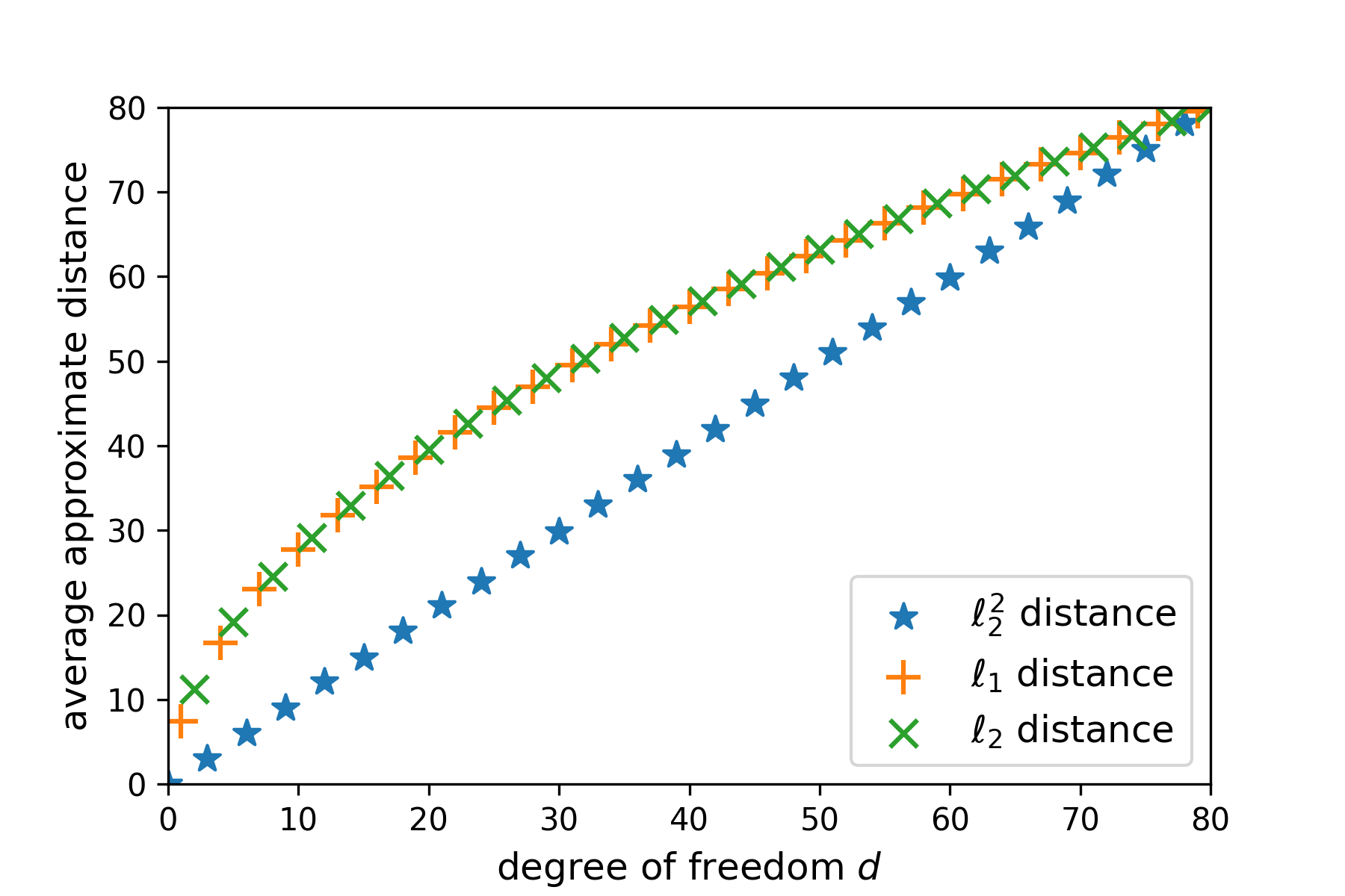
Figure 2: The average approximate distances with respect to the degree of freedom, from Monte Carlo simulations. The average squared Euclidean distance is linear to the degree of freedom, while the average $\ell_{1}$ and $\ell_{2}$ distances are not.

From Figure 2, it is straightforward to infer that the $\ell_{1}$ distance should perform as poorly as the $\ell_{2}$ distance. However, the experimental results in Table 1 show not only that the $\ell_{2}^{2}$ is the best among three, but also that the $\ell_{1}$ distance performs better than $\ell_{2}$ distance. A restriction on the orthogonal matrix $\bm{P}$ may answer this question. Recall that the distribution $Q(d,\bm{P})$ of the $\ell_{1}$ distance is related to both the orthogonal matrix $\bm{P}$ and the degree of freedom $d$. When the orthogonal matrix $\bm{P}$ is restricted to a signed permutation matrix, the distribution $Q(d,\bm{P})$ is a summation of the half-normal distributions $HN(1)$, and the expected value of the $\ell_{1}$ distance becomes linear with the degree $d$. The Monte Carlo simulation results are plotted in Figure 3 to illustrate the relationship between the average distances and the orthogonal matrix $\bm{P}$. From this figure, it can be confirmed that the $\ell_{1}$ distance has the potential to return an expected value equal to the degree of freedom. We speculate that the neural networks in the experiments of $\ell_{1}$ embedding learned that the latent matrix $\bm{P}$ obeys some restrictions, such as $\bm{P}$ as the signed permutation matrix, and lead to better performance compare to the $\ell_{2}$ distance.

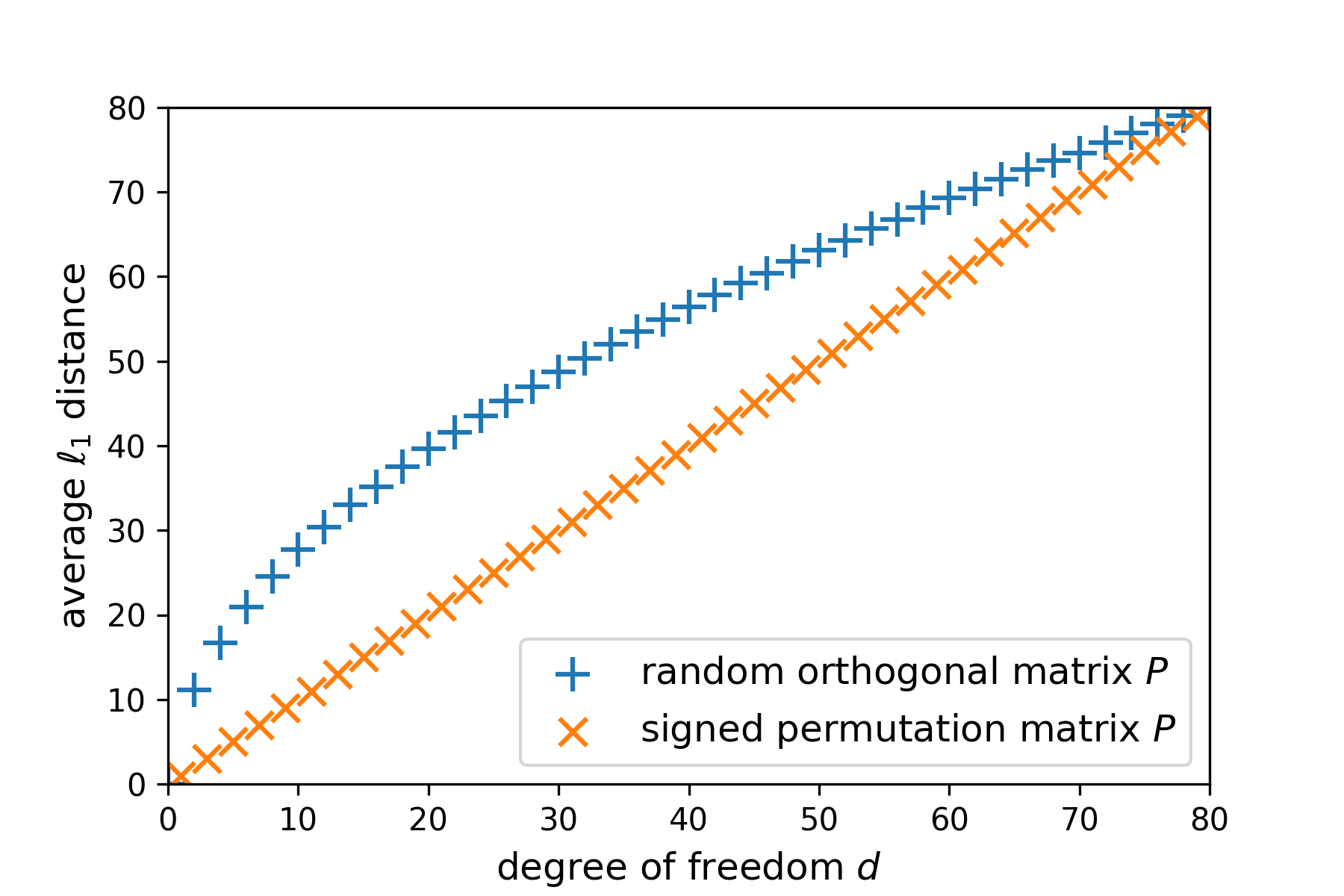
Figure 3: The average $\ell_{1}$ distances with respect to the degree of freedom under different choices of orthogonal matrix $\bm{P}$, from Monte Carlo simulations. The average $\ell_{1}$ distances with a signed permutation matrix $\bm{P}$ is linear to the degree of freedom, while the average $\ell_{1}$ distance with random orthogonal matrix $\bm{P}$ is not.

In summary, the theoretical results suggest that applying the squared Euclidean distance outperforms both $\ell_{1}$ and $\ell_{2}$ distances, and the $\ell_{1}$ distance is better than the $\ell_{2}$ distance. This is consistent with the experimental results in Table 1.

Appendix D Do these assumptions hold?

In Section 3.2, the following two of the three assumptions about the embedding vectors are mostly concerned in practice.

• The element $u_{i}$ of the embedding vector $\bm{u}$ is a random variable with a standard normal distribution $N(0,1)$.

• The elements $u_{i},u_{j}$ of the embedding vector $\bm{u}$ are expected to be independent of each other if $i\neq j$.

As mentioned in Section 3.2, the batch normalization is applied to the embedding vectors. The $\mathrm{BatchNorm}$ layer maintains the embedding element $u_{i}$ with $\mathrm{mean}\approx 0,\mathrm{std}\approx 1$ by updating the mean and variance per training batch with a momentum term. If the testing sample uses the same distribution as the training sample, the testing distribution for $u_{i}$ will also have $\mathrm{mean}\approx 0,\mathrm{std}\approx 1$. Since the normal distribution is the most common type, we speculate that the distribution of $u_{i}$ is close to the standard normal distribution $N(0,1)$ and no additional regularization is required. To verify our conjecture, we plot the distributions of the first $20$ elements of the embedding vector $\bm{u}$ from the testing phase in Figure 4. One could see that the distribution of each $u_{i}$ is close to $N(0,1)$, which suggests that the first assumption is reasonable and fits well with the real-world data.

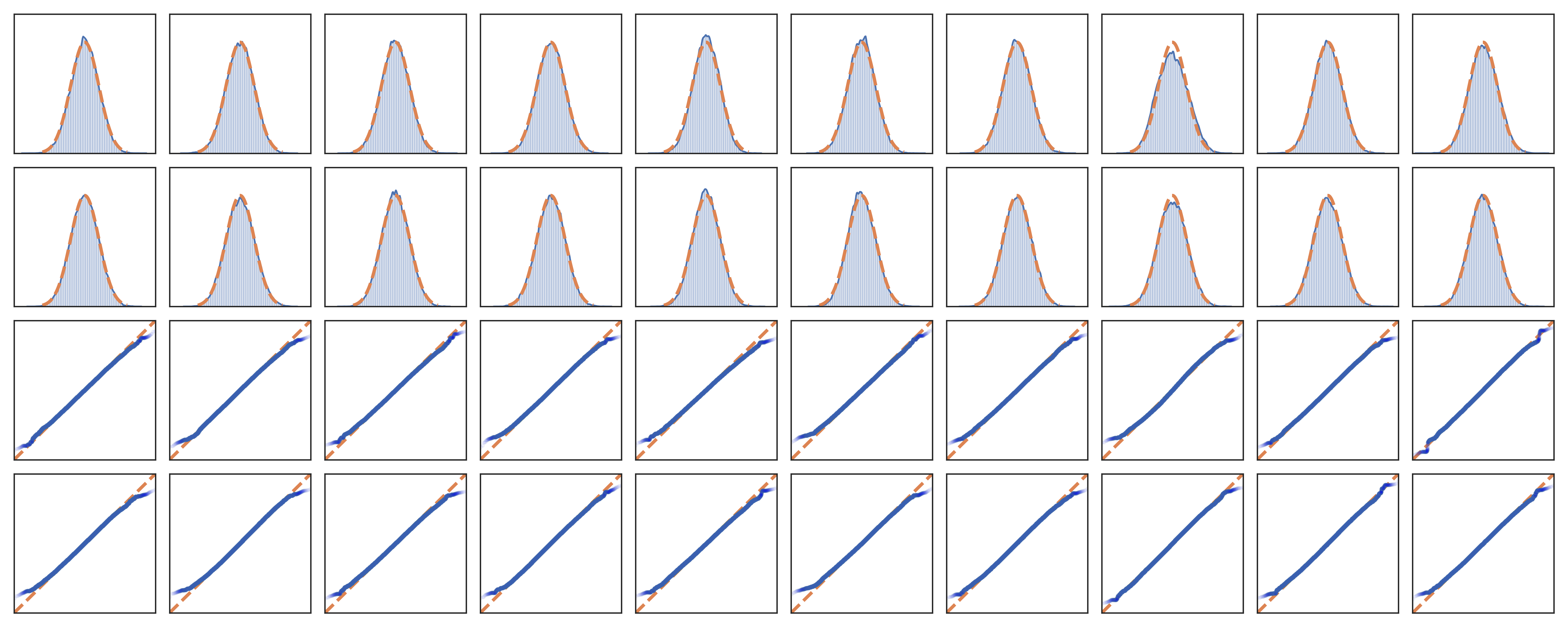
Figure 4: Distributions of the first $20$ elements of testing embedding vectors compared to $N(0,1)$. The upper subfigures are the estimated PDFs of the distributions of $u_{i}$s. The lower subfigures are the QQ plots of the $u_{i}$s. The orange dashed curves and lines are the PDF of $N(0,1)$ and the reference line to $N(0,1)$, respectively.

The elements of the embeddings are produced by the same neural network. It is straightforward to suspect that the different embedding elements $u_{i}$ and $u_{j}$ are not independent in practice. However, as analyzed below, the proposed approach declines the dependence between the embedding elements and upholds the assumption that $u_{i}$ and $u_{j}$ are independent if $i\neq j$. Let $\bm{u},\bm{v}$ be the rescaled embeddings of a pair of non-homologous sequences $\bm{s},\bm{t}$, respectively. By the proposed squared Euclidean embedding and RE$\chi^{2}$ loss, the degree of freedom with the difference between the embedding vectors $\bm{u}-\bm{v}$ is encouraged to meet $d_{L}(\bm{s},\bm{t})$, which is the ground truth Levenshtein distance between $\bm{s},\bm{t}$. In view of this, the degrees of freedom with the non-homologous $\bm{u}-\bm{v}$ are approximately equal to the average Levenshtein distance between non-homologous pairs and equal to the embedding dimension, suggesting that the embedding elements tend to be independent of each other. To show the independence of the embedding elements experimentally, we plot the heatmap of the Pearson correlation coefficient (PCC) between $u_{i}$ and $u_{j}$ from the testing phase of the proposed method (CNN-ED-5: $\ell_{2}^{2}$: RE$\chi^{2}$) in the left subfigure of Figure 5. This heatmap shows that most PCCs ($i\neq j$) have absolute values less than $0.2$, indicating that $u_{i}$ and $u_{j}$ are weakly or not correlated. To illustrate the effectiveness of the proposed method, the heatmap from the comparative/ablation experiment (CNN-ED-5: $\ell_{2}$: MSE) is plotted in the middle subfigure of Figure 5. We also plot the histograms of the PCCs from the proposed method and the ablation study in the right subfigure of Figure 5. From these heatmaps and histograms, we find that the independence decreases in the absence of the squared Euclidean embedding and RE$\chi^{2}$ loss. This partly confirms our analysis that the proposed approach reduces the dependence between the different embedding elements.

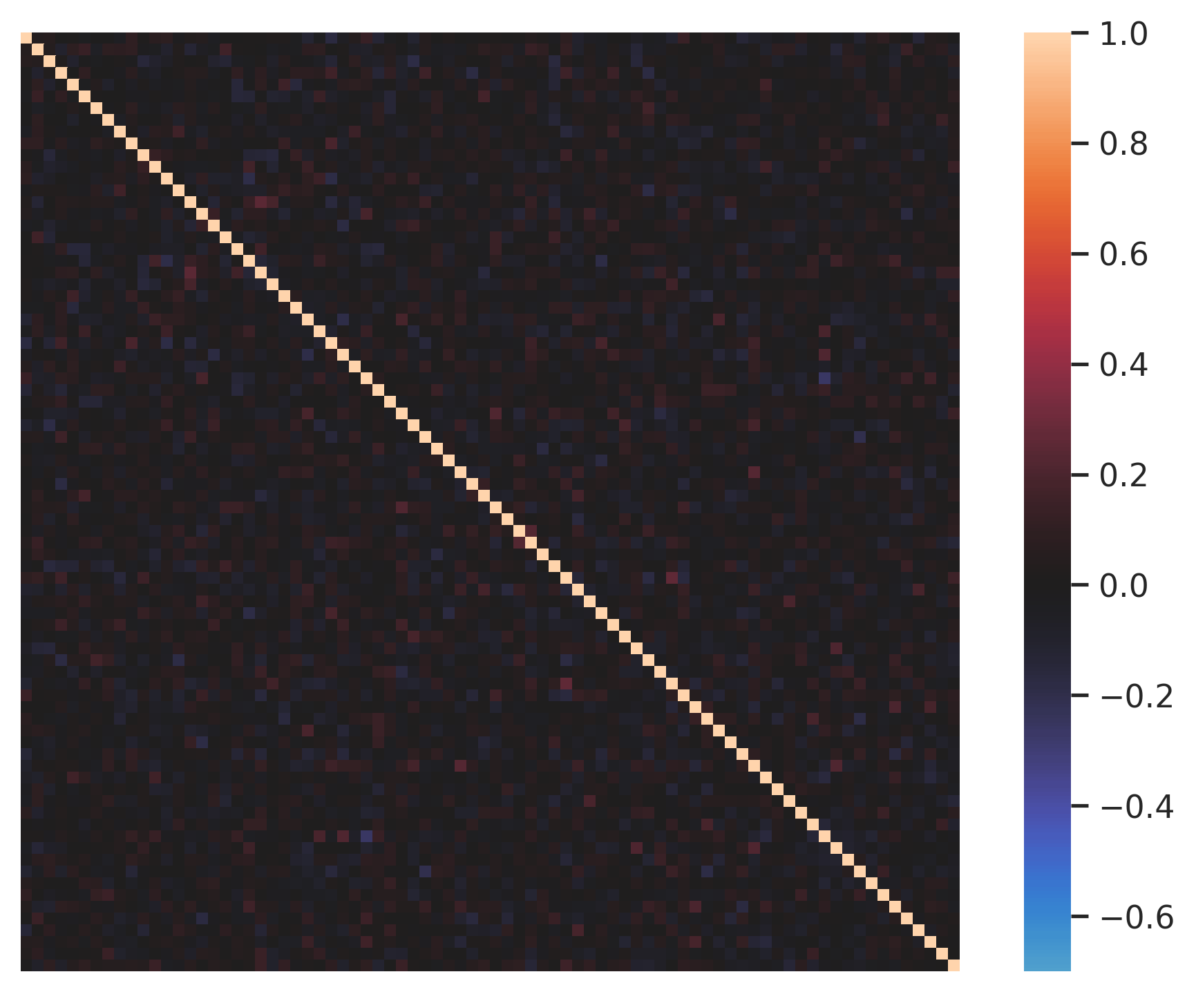
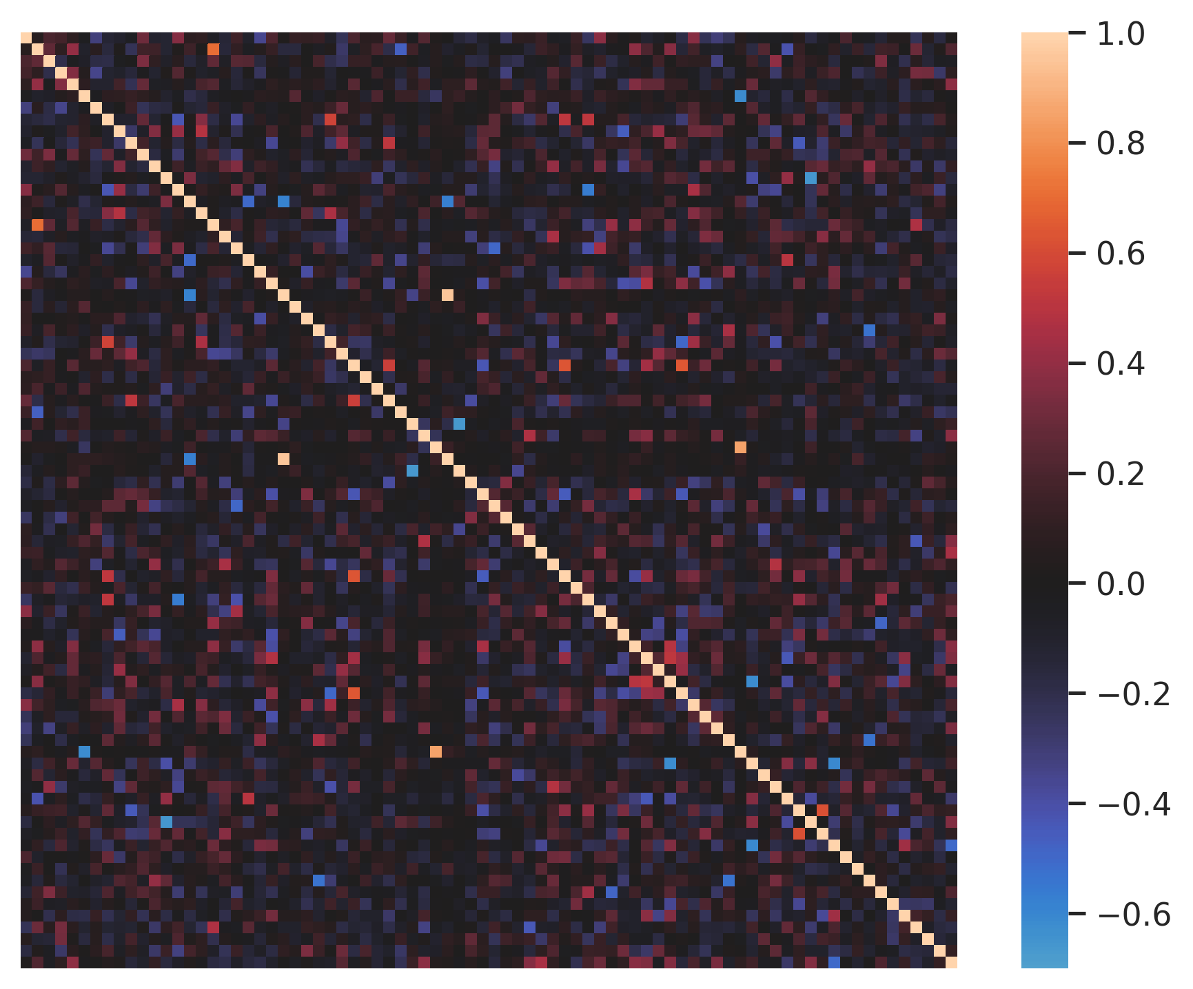
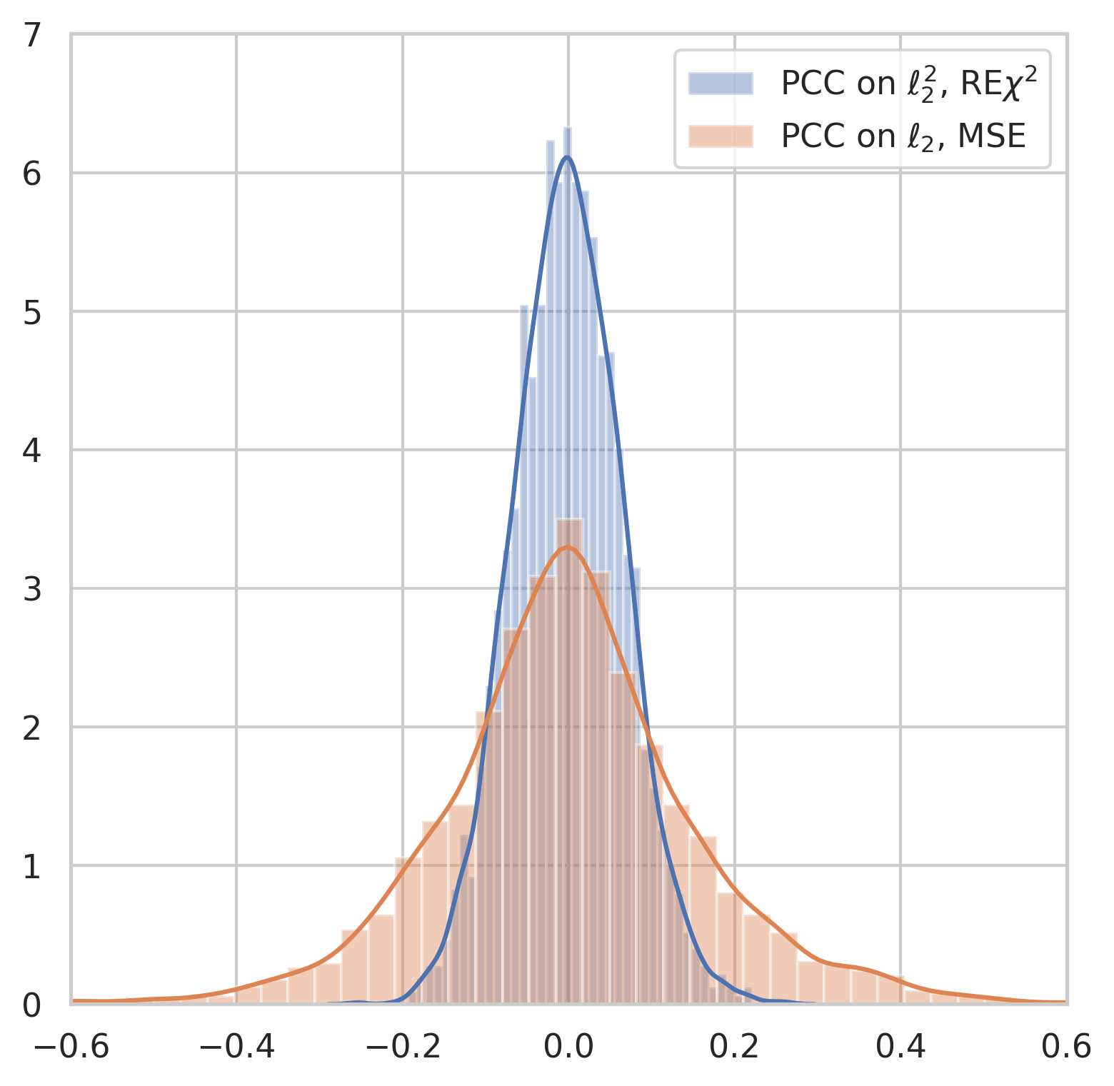
Figure 5: Heatmaps and distributions of the PCCs between different elements of embedding vectors. The left subfigure is the heatmap for the proposed method (CNN-ED-5: $\ell_{2}^{2}$: RE$\chi^{2}$). The middle subfigure is the heatmap for the comparative/ablation experiment (CNN-ED-5: $\ell_{2}$: MSE). The right subfigure is for the histograms of the PCCs for the two models (diagonal $1$s are omitted).

References

- Andoni et al. (2009) Andoni, A., Indyk, P., and Krauthgamer, R. Overcoming the non-embeddability barrier: Algorithms for product metrics. In Proceedings of the Twentieth Annual ACM-SIAM Symposium on Discrete Algorithms, pp. 865–874. SIAM, 2009.
- Backurs & Indyk (2015) Backurs, A. and Indyk, P. Edit Distance Cannot Be Computed in Strongly Subquadratic Time (Unless SETH is False). In Proceedings of the Forty-Seventh Annual ACM Symposium on Theory of Computing, STOC ’15, pp. 51–58, New York, NY, USA, 2015. Association for Computing Machinery. ISBN 9781450335362.
- Bar-Yossef et al. (2004) Bar-Yossef, Z., Jayram, T., Krauthgamer, R., and Kumar, R. Approximating edit distance efficiently. In 45th Annual IEEE Symposium on Foundations of Computer Science, pp. 550–559, 2004. doi: 10.1109/FOCS.2004.14.
- Blawat et al. (2016) Blawat, M., Gaedke, K., Hütter, I., Chen, X.-M., Turczyk, B., Inverso, S., Pruitt, B. W., and Church, G. M. Forward error correction for DNA data storage. Procedia Computer Science, 80:1011 – 1022, 2016. ISSN 1877-0509. International Conference on Computational Science 2016, ICCS 2016, 6-8 June 2016, San Diego, California, USA.
- Bromley et al. (1993) Bromley, J., Guyon, I., LeCun, Y., Säckinger, E., and Shah, R. Signature Verification Using a ”Siamese” Time Delay Neural Network. In Proceedings of the 6th International Conference on Neural Information Processing Systems, NIPS’93, pp. 737–744, San Francisco, CA, USA, 1993. Morgan Kaufmann Publishers Inc.
- Buhler (2001) Buhler, J. Efficient large-scale sequence comparison by locality-sensitive hashing . Bioinformatics, 17(5):419–428, 05 2001. ISSN 1367-4803. doi: 10.1093/bioinformatics/17.5.419.
- Chakraborty et al. (2016) Chakraborty, D., Goldenberg, E., and Koucký, M. Streaming algorithms for embedding and computing edit distance in the low distance regime. In Proceedings of the Forty-Eighth Annual ACM Symposium on Theory of Computing, STOC ’16, pp. 712–725, New York, NY, USA, 2016. Association for Computing Machinery. ISBN 9781450341325. doi: 10.1145/2897518.2897577.
- Charikar & Krauthgamer (2006) Charikar, M. and Krauthgamer, R. Embedding the ulam metric into . Theory of Computing, 2(11):207–224, 2006. doi: 10.4086/toc.2006.v002a011.
- Chen et al. (2021) Chen, W., Han, M., Zhou, J., Ge, Q., Wang, P., Zhang, X., Zhu, S., Song, L., and Yuan, Y. An artificial chromosome for data storage. National Science Review, 8(5), 02 2021. ISSN 2095-5138. doi: 10.1093/nsr/nwab028.
- Cho et al. (2014) Cho, K., van Merrienboer, B., Gülçehre, Ç., Bahdanau, D., Bougares, F., Schwenk, H., and Bengio, Y. Learning phrase representations using RNN encoder-decoder for statistical machine translation. In Moschitti, A., Pang, B., and Daelemans, W. (eds.), Proceedings of the 2014 Conference on Empirical Methods in Natural Language Processing, EMNLP 2014, pp. 1724–1734. ACL, 2014.
- Church et al. (2012) Church, G. M., Gao, Y., and Kosuri, S. Next-generation digital information storage in DNA. Science, 337(6102):1628–1628, 2012.
- Corso et al. (2021) Corso, G., Ying, Z., Pándy, M., Veličković, P., Leskovec, J., and Liò, P. Neural distance embeddings for biological sequences. In Ranzato, M., Beygelzimer, A., Dauphin, Y., Liang, P., and Vaughan, J. W. (eds.), Advances in Neural Information Processing Systems, volume 34, pp. 18539–18551. Curran Associates, Inc., 2021.
- Dai et al. (2020) Dai, X., Yan, X., Zhou, K., Wang, Y., Yang, H., and Cheng, J. Convolutional embedding for edit distance. In Proceedings of the 43rd International ACM SIGIR conference on research and development in Information Retrieval, SIGIR 2020, Virtual Event, China, July 25-30, 2020, pp. 599–608. ACM, 2020. doi: 10.1145/3397271.3401045.
- Datar et al. (2004) Datar, M., Immorlica, N., Indyk, P., and Mirrokni, V. S. Locality-sensitive hashing scheme based on p-stable distributions. In Proceedings of the Twentieth Annual Symposium on Computational Geometry, SCG ’04, pp. 253–262, New York, NY, USA, 2004. Association for Computing Machinery. ISBN 1581138857. doi: 10.1145/997817.997857.
- Dong et al. (2020) Dong, Y., Sun, F., Ping, Z., Ouyang, Q., and Qian, L. DNA storage: research landscape and future prospects. National Science Review, 7(6):1092–1107, 01 2020. ISSN 2095-5138. doi: 10.1093/nsr/nwaa007.
- Erlich & Zielinski (2017) Erlich, Y. and Zielinski, D. DNA Fountain enables a robust and efficient storage architecture. Science, 355(6328):950–954, 2017.
- Goldman et al. (2013) Goldman, N., Bertone, P., Chen, S., Dessimoz, C., LeProust, E. M., Sipos, B., and Birney, E. Towards practical, high-capacity, low-maintenance information storage in synthesized DNA. Nature, 494(7435):77–80, 2013. doi: 10.1038/nature11875.
- Grass et al. (2015) Grass, R. N., Heckel, R., Puddu, M., Paunescu, D., and Stark, W. J. Robust chemical preservation of digital information on DNA in silica with error-correcting codes. Angewandte Chemie International Edition, 54(8):2552–2555, 2015. doi: 10.1002/anie.201411378.
- Hanada et al. (2017) Hanada, H., Kudo, M., and Nakamura, A. On practical accuracy of edit distance approximation algorithms. arXiv preprint arXiv:1701.06134, 2017.
- Har-Peled et al. (2012) Har-Peled, S., Indyk, P., and Motwani, R. Approximate nearest neighbor: Towards removing the curse of dimensionality. Theory of Computing, 8(14):321–350, 2012. doi: 10.4086/toc.2012.v008a014.
- Hartigan & Wong (1979) Hartigan, J. A. and Wong, M. A. Algorithm as 136: A k-means clustering algorithm. Journal of the Royal Statistical Society. Series C (Applied Statistics), 28(1):100–108, 1979. ISSN 00359254, 14679876.
- Kingma & Ba (2015) Kingma, D. P. and Ba, J. Adam: A method for stochastic optimization. In Bengio, Y. and LeCun, Y. (eds.), 3rd International Conference on Learning Representations, ICLR 2015, San Diego, CA, USA, May 7-9, 2015, Conference Track Proceedings, 2015.
- Krizhevsky et al. (2012) Krizhevsky, A., Sutskever, I., and Hinton, G. E. Imagenet classification with deep convolutional neural networks. In Pereira, F., Burges, C. J. C., Bottou, L., and Weinberger, K. Q. (eds.), Advances in Neural Information Processing Systems 25, pp. 1097–1105. Curran Associates, Inc., 2012.
- Kullback & Leibler (1951) Kullback, S. and Leibler, R. A. On information and sufficiency. The Annals of Mathematical Statistics, 22(1):79–86, 1951. ISSN 00034851.
- LeCun et al. (2015) LeCun, Y., Bengio, Y., and Hinton, G. Deep learning. Nature, 521(7553):436–444, 2015. doi: 10.1038/nature14539.
- Levenshtein (1966) Levenshtein, V. I. Binary codes capable of correcting deletions, insertions, and reversals. In Soviet physics doklady, volume 10, pp. 707–710, 1966.
- Masek & Paterson (1980) Masek, W. J. and Paterson, M. S. A faster algorithm computing string edit distances. Journal of Computer and System Sciences, 20(1):18–31, 1980. ISSN 0022-0000. doi: https://doi.org/10.1016/0022-0000(80)90002-1.
- Organick et al. (2018) Organick, L., Ang, S. D., Chen, Y.-J., Lopez, R., Yekhanin, S., Makarychev, K., Racz, M. Z., Kamath, G., Gopalan, P., Nguyen, B., et al. Random access in large-scale DNA data storage. Nature biotechnology, 36(3):242–248, 2018.
- Ostrovsky & Rabani (2007) Ostrovsky, R. and Rabani, Y. Low distortion embeddings for edit distance. J. ACM, 54(5):23–es, October 2007. ISSN 0004-5411. doi: 10.1145/1284320.1284322.
- Ping et al. (2019) Ping, Z., Ma, D., Huang, X., Chen, S., Liu, L., Guo, F., Zhu, S. J., and Shen, Y. Carbon-based archiving: current progress and future prospects of DNA-based data storage. GigaScience, 8(6), 06 2019. ISSN 2047-217X. doi: 10.1093/gigascience/giz075. giz075.
- (31) Rasheed, Z., Rangwala, H., and Barbará, D. Efficient clustering of metagenomic sequences using locality sensitive hashing. In Proceedings of the 2012 SIAM International Conference on Data Mining (SDM), pp. 1023–1034. doi: 10.1137/1.9781611972825.88.
- Rashtchian et al. (2017) Rashtchian, C., Makarychev, K., Racz, M., Ang, S., Jevdjic, D., Yekhanin, S., Ceze, L., and Strauss, K. Clustering Billions of Reads for DNA Data Storage. In Guyon, I., Luxburg, U. V., Bengio, S., Wallach, H., Fergus, R., Vishwanathan, S., and Garnett, R. (eds.), Advances in Neural Information Processing Systems, volume 30. Curran Associates, Inc., 2017.
- Robbins & Monro (1951) Robbins, H. and Monro, S. A stochastic approximation method. The Annals of Mathematical Statistics, 22(3):400–407, 1951. ISSN 00034851.
- Rumelhart et al. (1985) Rumelhart, D. E., Hinton, G. E., and Williams, R. J. Learning internal representations by error propagation. Technical report, California Univ San Diego La Jolla Inst for Cognitive Science, 1985.
- Schroff et al. (2015) Schroff, F., Kalenichenko, D., and Philbin, J. Facenet: A unified embedding for face recognition and clustering. In Proceedings of the IEEE Conference on Computer Vision and Pattern Recognition (CVPR), June 2015.
- Sokolov (2007) Sokolov, A. Vector representations for efficient comparison and search for similar strings. Cybernetics and Systems Analysis, 43(4):484–498, 2007.
- Ukkonen (1992) Ukkonen, E. Approximate string-matching with q-grams and maximal matches. Theoretical Computer Science, 92(1):191–211, 1992. ISSN 0304-3975. doi: https://doi.org/10.1016/0304-3975(92)90143-4.
- Wang et al. (2014) Wang, J., Shen, H. T., Song, J., and Ji, J. Hashing for similarity search: A survey. arXiv preprint arXiv:1408.2927, 2014.
- Yu et al. (2016) Yu, M., Li, G., Deng, D., and Feng, J. String similarity search and join: a survey. Frontiers of Computer Science, 10(3):399–417, 2016.
- Yuan et al. (2014) Yuan, P., Sha, C., and Sun, Y. Hashed-join: Approximate string similarity join with hashing. In Han, W.-S., Lee, M. L., Muliantara, A., Sanjaya, N. A., Thalheim, B., and Zhou, S. (eds.), Database Systems for Advanced Applications, pp. 217–229, Berlin, Heidelberg, 2014. Springer Berlin Heidelberg. ISBN 978-3-662-43984-5.
- Zhang & Zhang (2017) Zhang, H. and Zhang, Q. Embedjoin: Efficient edit similarity joins via embeddings. In Proceedings of the 23rd ACM SIGKDD International Conference on Knowledge Discovery and Data Mining, KDD ’17, pp. 585–594, New York, NY, USA, 2017. Association for Computing Machinery. ISBN 9781450348874. doi: 10.1145/3097983.3098003.
- Zhang et al. (2020) Zhang, X., Yuan, Y., and Indyk, P. Neural embeddings for nearest neighbor search under edit distance, 2020.