Hercules: Boosting the Performance of Privacy-preserving Federated Learning

Abstract

In this paper, we address the problem of privacy-preserving federated neural network training with $N$ users. We present Hercules, an efficient and high-precision training framework that can tolerate collusion of up to $N-1$ users. Hercules follows the POSEIDON framework proposed by Sav et al. (NDSS’21), but makes a qualitative leap in performance with the following contributions: (i) we design a novel parallel homomorphic computation method for matrix operations, which enables fast Single Instruction and Multiple Data (SIMD) operations over ciphertexts. For the multiplication of two $h\times h$ dimensional matrices, our method reduces the computation complexity from $O(h^{3})$ to $O(h)$. This greatly improves the training efficiency of the neural network since the ciphertext computation is dominated by the convolution operations; (ii) we present an efficient approximation on the sign function based on the composite polynomial approximation. It is used to approximate non-polynomial functions (i.e., ReLU and max), with the optimal asymptotic complexity. Extensive experiments on various benchmark datasets (BCW, ESR, CREDIT, MNIST, SVHN, CIFAR-10 and CIFAR-100) show that compared with POSEIDON, Hercules obtains up to $4\%$ increase in model accuracy, and up to $60\times$ reduction in the computation and communication cost.

1 Introduction

As a promising neural network training mechanism, Federated Learning (FL) has been highly sought after with some attractive features including amortized overhead and mitigation of privacy threats. However, the conventional FL setup has some inherent privacy issues [1, 2]. Consider a scenario where a company (referred to as the cloud server) pays multiple users and requires them to train a target neural network model collaboratively. Although each user is only required to upload the intermediate data (e.g., gradients) instead of the original training data to the server during the training process, a large amount of sensitive information can still be leaked implicitly from these intermediate values. Previous works have demonstrated many powerful attacks to achieve this, such as attribute inference attacks and gradient reconstruction attacks [3, 4, 5]. On the other hand, the target model is locally distributed to each user according to the FL protocol, which ignores the model privacy and may be impractical in real-world scenarios. Actually, to protect the model privacy, the server must keep users ignorant of the details of the model parameters throughout the training process.

1.1 Related Works

Extensive works have been proposed to mitigate the above privacy threats. In general, existing privacy-preserving deep learning solutions mainly rely on the following two lines of technologies: Differential Privacy (DP) [6, 7] and crypto-based multiparty secure computing (MPC) [8, 9, 10, 11, 12]. Each one has merits and demerits depending on the scenario to which it is applied.

Differential Privacy. DP is usually applied in the training phase [6, 7]. To ensure the indistinguishability between individual samples while maintaining high training accuracy, each user is required to add noise to the gradient or local parameters that meets the preset privacy budget. Abadi et al. [6] propose the first differentially private stochastic gradient descent (SGD) algorithm. They carefully implement gradient clipping, hyperparameter tuning, and moment accountant to obtain a tight estimate of overall privacy loss, both asymptotically and empirically. Yu et al. [7] design a new DP-SGD, which employs a new primitive called zero concentrated differential privacy (zCDP) for privacy accounting, to achieve a rigorous estimation of the privacy loss. In recent years, many variants of the above works have been designed and applied to specific scenarios [13, 14, 15, 16]. Most of them follow the principle that the minimum accumulated noise is added to the gradient or local parameters while meeting the preset privacy budget.

DP is cost-effective because each user is only required to add noise that obeys a specific distribution during training. However, it is forced to make a trade-off between training accuracy and privacy, i.e., a strong privacy protection level can be reached at the cost of certain model accuracy drop [17, 18]. This goes against the motivation of this paper, as our goal is to design a highly secure FL training framework without compromising the model accuracy.

Crypto-based multiparty secure computing. The implementation of this strategy mainly relies on two general techniques, secret sharing [19] and homomorphic encryption (HE) [11]. MPC enables the calculation of arbitrary functions collaboratively by multiple parties without revealing the secret input of each party. To support privacy-preserving neural network training, most existing works [19, 20, 8, 9, 10] rely on splitting the training task into two or more servers, who are usually assumed to be non-colluding. Then, state-of-the-art secret sharing methods, including arithmetic sharing [19], boolean sharing [8], and Yao’s garbled circuit [21] are carefully integrated to efficiently implement various mathematical operations under the ciphertext. Mohassel et al. [20] propose SecureML, the first privacy-preserving machine learning framework for generalized linear model regression and neural network training. It lands on the setting of two non-colluding servers, where users securely outsource local data to them. Then, several types of secret sharing methods are mixed and used to complete complex ciphertext operations. Other works, e.g., ABY³ [8], QUOTIENT[9], BLAZE [22], Trident[23], are also exclusively based on the MPC protocol between multiple non-colluding servers (or a minority of malicious servers) to achieve fast model training and prediction.

It is cost-effective to outsource the training task among multiple users to several non-colluding servers, avoiding the high communication overhead across large-scale users. However, it may be impractical in real scenarios where the setting of multiple servers is not available. Especially in FL scenarios, users are more inclined to keep their datasets locally rather than uploading data to untrusted servers. To alleviate this problem, several works [11, 12, 2, 24] propose to use multi-party homomorphic encryption (a.k.a. threshold homomorphic encryption, as a variant of the standard HE), as the underlying technology to support direct interactions among multiple data owners for distributed learning. For example, Zheng et al. [11] present Helen, a secure distributed learning approach for linear models, where the threshold Paillier scheme [25] is used to protect users’ local data. Froelicher et al. [24] reduce the computation overhead of Helen by using the packed plaintext encoding with the SIMD technology [2]. Sav et al. propose POSEIDON [12], the first distributed training framework with multi-party homomorphic encryption. It relies on the multiparty version of the CKKS (MCKKS) cryptosystem [26] to encrypt users’ local data. Compared with the standard CKKS, the secret key of MCKKS is securely shared with multiple entities. As a result, each entity still performs the function evaluation under the same public key. However, the decryption of the result requires the participation of all entities. Besides, non-polynomial functions are approximated as polynomial functions to be efficiently executed by CKKS.

1.2 Technical Challenges

In this paper, we follow the specifications of POSEIDON to design our FL training framework, because such a technical architecture enables the users’ data to be kept locally without incurring additional servers. However, there are still several critical issues that have not been solved well. (1) Computation overhead is the main obstacle hindering the development of HE. It usually requires more computing resources to perform the same machine learning tasks compared to outsourcing-based solutions [8, 9, 10]. Although there are some optimization methods such as parameter quantization and model compression [9, 27], they inevitably degrade the model accuracy. Recently, Zhang et al. [28] design GALA, which employs a novel coding technique for matrix-vector multiplication. In this way, multiple plaintexts are packed into one ciphertext to perform efficient homomorphic SIMD operations without reducing the calculation accuracy. However, GALA is specifically designed for the MPC protocol that uses a mixture of HE and garbled circuits, and its effectiveness is highly dependent on the assistance of the inherent secret sharing strategy. Therefore, it is necessary to design a computation optimization method that is completely suitable for HE, without sacrificing the calculation accuracy. (2) There is a lack of satisfactory approximation mechanisms for non-polynomial functions in HE. HE basically supports homomorphic addition and multiplication. For non-polynomial functions, especially ReLU, one of the most popular activation functions in hidden layers, we need to approximate them to polynomials for ciphertext evaluation. The common polynomial approximation method, such as the minimax method, aims to find the approximate polynomial with the smallest degree on the objective function under the condition of a given error bound. However, the computation complexity of evaluating these polynomials is enormous, making it quite inefficient to obtain the fitting function with high-precision [29, 30]. Recently, Lu et al. [31] propose PEGASUS, which can efficiently switch back and forth between a packed CKKS ciphertext and FHEW ciphertext [32] without decryption, allowing us to evaluate both polynomial and non-polynomial functions on encrypted data. However, its performance is still far from practical.

1.3 Our Contributions

As discussed above, the HE-based FL is more in line with the needs of most real-world applications, compared to other methods. However, it suffers from computing bottlenecks and poor compatibility with non-polynomial functions. To mitigate these limitations, we present Hercules, an efficient, privacy-preserving and high-precision framework for FL. Hercules follows the tone of the state-of-the-art work POSEIDON [12], but makes a qualitative leap in performance. Specifically, we first devise a new method for parallel homomorphic computation of matrix, which supports fast homomorphic SIMD operations, including addition, multiplication, and transposition. Then, instead of fitting the replacement function of ReLU for training in POSEIDON, we design an efficient method based on the composite polynomial approximation. In short, the contributions of Hercules are summarized as follows:

• We design a new method to execute matrix operations in parallel, which can pack multiple plaintexts into a ciphertext to achieve fast homomorphic SIMD operations (Section 3). Our key insight is to minimize the number of plaintext slots that need to be rotated in matrix multiplication through customized permutations. Compared with existing works [12, 33], our solution reduces the computation complexity from $O(h^{3})$ to $O(h)$ for the multiplication of any two $h\times h$ matrices. It greatly improves the neural network training efficiency since the ciphertext computation is dominated by the convolution operations. We describe the detail of efficiently executing matrix transposition on packed ciphertexts, and packing multiple matrices into one ciphertext, yielding better-amortized performance.

• We present an efficient approximation on the sign function based on the composite polynomial approximation, with optimal asymptotic complexity (Section 4). The core of our solution is to carefully construct a polynomial $g$ with a constant degree, and then make the composite polynomial $g\circ g\circ g\circ\cdots\circ g$ infinitely close to the sign function, as the number of $g$ increases. In this way, our new algorithm only requires $\Theta(\log(1/\delta))+\Theta(\log\sigma)$ computation complexity to obtain an approximate sign function result of $m\in[-1,-\delta]\cup[\delta,1]$ within $2^{-\sigma}$ error. For example, for an encrypted 20-bit integer $m$, we can obtain the result of the sign function within $2^{-20}$ error with an amortized running time of 20.05 milliseconds, which is $33\times$ faster than the state-of-the-art work [34].

• We show that Hercules provides semantic security in the FL scenario consisting of $N$ users and a parameter server, and tolerates collusion among up to $N-1$ passive users (Section 5). This is mainly inherited from the property of the MCKKS.

• We conduct extensive experiments on various benchmark datasets (BCW, ESR, CREDIT, MNIST, SVHN, CIFAR-10 and CIFAR-100) to demonstrate the superiority of Hercules in terms of classification accuracy, and overhead of computation and communication (Section 6). Specifically, compared with POSEIDON, we obtain up to $4\%$ increase in model accuracy, and up to $60\times$ reduction in the computation and communication cost.

Roadmap: In Section 2, we review some basic concepts used in this paper, and introduce the scenarios and threat models. In Sections 3 to 5, we give the details of Hercules. Performance evaluation is presented in 6. Section 7 concludes the paper.

2 Preliminaries

2.1 Neural Network Training

A neural network usually consists of an input layer, one or more hidden layers, and an output layer, where hidden layers include convolutional layers, pooling layers, activation function layers, and fully connected layers. The connections between neurons in adjacent layers are parameterized by ${\omega}$ (i.e., model parameters), and each neuron is associated with an element-wise activation function $\varphi$ (such as sigmoid, ReLU, and softmax). Given the training sample set $({x},{y})\in D$, training a neural network of $\mathbb{L}$ layers is generally divided into two phases: feedforward and backpropagation. Specifically, at the $k$-th iteration, the weights between layers $j$ and $j+1$ are denoted as a matrix ${\omega}_{j}^{k}$; matrix $M_{j}$ represents the activation of neurons in the $j$-th layer. Then the input ${x}$ is sequentially propagated to each layer with operations of linear transformation (i.e, $E_{j}^{k}={\omega}_{j}^{k}\times M_{j-1}^{k}$) and non-linear transformation (i.e., $M_{j}^{k}=\varphi(E_{j}^{k})$) to obtain the final classification result ${\bar{y}}=M_{\mathbb{L}}^{k}$. With the loss function ${L}$ which is usually set as ${L}$=$||{y}-\bar{{y}}||_{2}$, the mini-batch based Stochastic Gradient Descent (SGD) algorithm [12] is exploited to optimize the parameter ${\omega}$. The parameter update rule is ${\omega}_{j}^{k+1}={\omega}_{j}^{k}-\frac{\eta}{\mathcal{B}}\bigtriangledown{\omega}_{j}^{k}$, where $\eta$ and $\mathcal{B}$ indicate the learning rate and the random batch size of input samples, and $\bigtriangledown{\omega}_{j}^{k}=\frac{\partial L}{\partial{\omega}_{j}^{k}}$. Since the transposition of matrices/vectors is involved in the backpropagation, we use $V^{T}$ to represent the transposition of variable $V$. The feedforward and backpropagation steps are performed iteratively until the neural network meets the given convergence constraint. The detailed implementation is shown in Algorithm 1.

Algorithm 1 Mini-batch based SGD algorithm

0:  ${\omega}_{1}^{k},{\omega}_{2}^{k},\cdots,{\omega}_{\mathbb{L}}^{k}$.

0:  ${\omega}_{1}^{k+1},{\omega}_{2}^{k+1},\cdots,{\omega}_{\mathbb{L}}^{k+1}$.

1:  for $t=1$ to $\mathcal{B}$ do

2:     $M_{0}=X[t]$         $\rhd$ feedforward

3:     for $j=1$ to $\mathbb{L}$ do

4:        $E_{j}^{k}={\omega}_{j}^{k}\times M_{j-1}^{k}$

5:        $M_{j}^{k}=\varphi(E_{j}^{k})$

6:     end for

7:     $L_{\mathbb{L}}^{k}=||y[t]-M_{\mathbb{L}}^{k}||_{2}$    $\rhd$ backpropagation

8:     $L_{\mathbb{L}}^{k}=\varphi^{\prime}(E_{\mathbb{L}}^{k})\odot L_{\mathbb{L}}^{k}$

9:     $\bigtriangledown{\omega}_{\mathbb{L}}^{k}+=(M_{\mathbb{L}-1}^{k})^{T}\times L_{\mathbb{L}}^{k}$

10:     for $j=\mathbb{L}-1$ to $1$ do

11:        $L_{j}^{k}=L_{j+1}^{k}\times(\omega_{j+1}^{k})^{T}$

12:        $L_{j}^{k}=\varphi^{\prime}(E_{j}^{k})\odot L_{j}^{k}$

13:        $\bigtriangledown{\omega}_{j}^{k}+=(M_{j-1}^{k})^{T}\times L_{j}^{k}$

14:     end for

15:  end for

16:  for $j=1$ to $\mathbb{L}$ do

17:     ${\omega}_{j}^{k+1}={\omega}_{j}^{k}-\frac{\eta}{\mathcal{B}}\bigtriangledown{\omega}_{j}^{k}$

18:  end for

2.2 Multiparty Version of CKKS

Hercules relies on the multiparty version of Cheon-Kim-Kim-Song (MCKKS) [12] fully homomorphic encryption to protect users’ data as well as the model’s parameter privacy. Compared with the standard CKKS, the secret key of MCKKS is securely shared with all entities. As a result, each entity still performs ciphertext evaluation under the same public key, while the decryption of the result requires the participation of all entities. As shown in [12], MCKKS has several attractive properties: (i) it is naturally suitable for floating-point arithmetic circuits, which facilitates the implementation of machine learning; (ii) it flexibly supports collaborative computing among multiple users without revealing the respective share of the secret key; (iii) it supports the function of key-switch, making it possible to convert a ciphertext encrypted under a public key into a ciphertext under another public key without decryption. Such a property facilitates the decryption of ciphertexts collaboratively. We provide a short description of MCKKS and list all the functions required by Hercules in Figure 1. Informally, given a cyclotomic polynomial ring with a dimension of $\mathcal{N}$, the plaintext and ciphertext space of MCKKS is defined as $R_{Q_{\mathcal{L}}}=\mathbb{Z}_{Q_{\mathcal{L}}}[X]/(X^{\mathcal{N}}+1)$, where $Q_{\mathcal{L}}=\prod_{0}^{\mathcal{L}}q_{i}$, and each $q_{i}$ is a unique prime. $Q_{\mathcal{L}}$ is the ciphertext module under the initial level $\mathcal{L}$. In CKKS, a plaintext vector with up to $\mathcal{N}/2$ values can be encoded into a ciphertext. As shown in Figure 1, given a plaintext $m\in R_{Q_{\mathcal{L}}}$ (or a plaintext vector $\mathbf{m}=(m_{1},\cdots,m_{n})\in R_{Q_{\mathcal{L}}}^{n}$, with $n\leq\mathcal{N}/2$) with its encoded (packed) plaintext $\hat{m}$, the corresponding ciphertext is denoted as $[\mathbf{c}]_{pk}=(c_{1},c_{2})\in R_{Q_{\mathcal{L}}}^{2}$. Besides, we use symbols $\mathcal{L}_{\mathbf{c}_{pk}}$, $\Delta_{\mathbf{c}_{pk}}$, $\mathcal{L}$, $\Delta$ to indicate the current level of $[\mathbf{c}]_{pk}$, the current scale of $\mathbf{c}$, the initial level, and the initial scale of a fresh ciphertext, respectively. All functions named starting with $\mathbf{D}$ (except for $\mathbf{Dcd}(\cdot)$) in Figure 1 need to be executed cooperatively by all the users, while the rest operations can be executed locally by each user with the public key. For more details about MCKKS, please refer to literature [12, 24, 1].

1) $\mathbf{SecKeyGen}(1^{\lambda})$: Given a security parameter $\lambda$, output a secret key $sk_{i}$ for each user $i\in[N]$, where $[N]$ is the shorthand $\{1,2,\cdots N\}$ and $\sum_{i=1}^{i=N}sk_{i}=sk$. 2) $\mathbf{DKeyGen}(\{sk_{i}\})$: Given the set of secret keys $\{sk_{i}\}$, $i\in[N]$, output the collective public key $pk$. 3) $\mathbf{Ecd}(\cdot)$: Given a plaintext $m$ (or a plaintext vector $\mathbf{m}$ whose dimension does not exceed $\mathcal{N}/2$), output the encoded (packed) plaintext $\hat{m}\in R_{Q_{\mathcal{L}}}$, with scale $\Delta$. 4) $\mathbf{Dcd}(\hat{m})$: Given an encoded (packed) plaintext $\hat{m}\in R_{Q_{\mathcal{L}_{m}}}$ with scale $\Delta_{m}$, output the decoding of $m$ (or the plaintext vector $\mathbf{m}$). 5) $\mathbf{Enc}(pk,\hat{m})$: Given the collective public key $pk$, and an encoded (packed) plaintext $\hat{m}\in R_{Q_{\mathcal{L}}}$, output the ciphertext $\mathbf{[c]}_{pk}\in R_{Q_{\mathcal{L}}}^{2}$ with scale $\Delta$. 6) $\mathbf{DDec}(\mathbf{[c]}_{pk},\{sk_{i}\})$: Given a ciphertext $\mathbf{[c]}_{pk}\in R_{Q_{\mathcal{L}_{\mathbf{c}}}}^{2}$ with scale $\Delta_{\mathbf{c}_{pk}}$, and the set of secret keys $\{sk_{i}\}$, $i\in[1,N]$, output the plaintext $p\in R_{Q_{\mathcal{L}_{\mathbf{c}}}}$ with scale $\Delta_{\mathbf{c}_{pk}}$. 7) $\mathbf{Add}(\mathbf{[c]}_{pk},\mathbf{[c^{\prime}]}_{pk})$: Given two ciphertexts $\mathbf{[c]}_{pk}$ and $\mathbf{[c^{\prime}]}_{pk}$ encrypted with the same public key $pk$, output $[\mathbf{c}+\mathbf{c^{\prime}}]_{pk}$ with level $\min(\mathcal{L}_{\mathbf{c}_{pk}},\mathcal{L}_{\mathbf{c}^{\prime}_{pk}})$ and scale $\max(\Delta_{\mathbf{c}_{pk}},\Delta_{\mathbf{c}^{\prime}_{pk}})$. 8) $\mathbf{Sub}(\mathbf{[c]}_{pk},\mathbf{[c^{\prime}]}_{pk})$: Given two ciphertexts $\mathbf{[c]}_{pk}$ and $\mathbf{[c^{\prime}]}_{pk}$, output $[\mathbf{c}-\mathbf{c}^{\prime}]_{pk}$ with level $\min(\mathcal{L}_{\mathbf{c}_{pk}},\mathcal{L}_{\mathbf{c}^{\prime}_{pk}})$ and scale $\max(\Delta_{\mathbf{c}_{pk}},\Delta_{\mathbf{c}^{\prime}_{pk}})$. 9) $\mathbf{Mul}_{pt}([\mathbf{c}]_{pk},\hat{m})$: Given a ciphertext $[\mathbf{c}]_{pk}$ and an encoded (packed) plaintext $\hat{m}$, output $[\mathbf{c}m]_{pk}$ with level $\min(\mathcal{L}_{\mathbf{c}_{pk}},\mathcal{L}_{\mathbf{c}^{\prime}_{pk}})$ and scale $\Delta_{\mathbf{c}_{pk}}\times\Delta_{m}$. 10) $\mathbf{Mul}_{ct}([\mathbf{c}]_{pk},[\mathbf{c}^{\prime}]_{pk})$: Given two ciphertexts $[\mathbf{c}]_{pk}$ and $[\mathbf{c}^{\prime}]_{pk}$, output $[\mathbf{c}\mathbf{c}^{\prime}]_{pk}$ with level $\min(\mathcal{L}_{\mathbf{c}_{pk}},\mathcal{L}_{\mathbf{c}^{\prime}_{pk}})$ and scale $\Delta_{\mathbf{c}_{pk}}\times\Delta_{\mathbf{c}^{\prime}_{pk}}$. 11) $\mathbf{Rot}([\mathbf{c}]_{pk},k)$: Given a ciphertexts $[\mathbf{c}]_{pk}$, homomorphically rotate $[\mathbf{c}]_{pk}$ to the right ($k>0$) or to the left ($k<0$) by $k$ times. 12) $\mathbf{RS}([\mathbf{c}]_{pk})$: Given a ciphertexts $[\mathbf{c}]_{pk}$, output $[\mathbf{c}]_{pk}$ with scale $\Delta_{\mathbf{c}}/q_{\Delta_{\mathbf{c}}}$ and level $\mathcal{L}_{\mathbf{c}}-1$. 13) $\mathbf{DKeySwitch}([\mathbf{c}]_{pk},pk^{\prime},\{sk_{i}\})$: Given a ciphertexts $[\mathbf{c}]_{pk}$, another public key $pk^{\prime}$, and the set of secret keys $\{sk_{i}\}$, $i\in[N]$, output $[\mathbf{c}]_{pk^{\prime}}$. 14) $\mathbf{DBootstrap}([\mathbf{c}]_{pk},\mathcal{L}_{\mathbf{c}_{pk}},\Delta_{\mathbf{c}_{pk}},\{sk_{i}\})$: Given a ciphertexts $[\mathbf{c}]_{pk}$ with level $\mathcal{L}_{\mathbf{c}_{pk}}$ and scale $\Delta_{\mathbf{c}_{pk}}$, and the set of secret keys $\{sk_{i}\}$, $i\in[N]$, output $[\mathbf{c}]_{pk}$ with initial $\mathcal{L}$ and scale $\Delta$.

Fig. 1: Cryptographic operations of MCKKS

2.3 Threat Model and Privacy Requirements

We consider a FL scenario composed of a parameter server and $N$ users for training a neural network model collaboratively. Specifically, the server (also the model owner) first initializes the target model $\mathcal{M}$ and broadcasts the encrypted model $[\mathbf{M}]_{pk}=\mathbf{Enc}(pk,\mathcal{M})$ (i.e., encrypting all the model parameters) to all the users. Then, each user $P_{i}$ with a dataset $\{x,y\}\in D_{i}$ trains $[\mathbf{M}]_{pk}$ locally using the mini-batch SGD algorithm and then sends the encrypted local gradients to the server. After receiving the gradients from all the users, the server homomorphically aggregates them and broadcasts back the global model parameters. All the participants perform the above process iteratively until the model converges. Since the final trained model is encrypted with the public key $pk$, for the accessibility of the server to the plaintext model, we rely on the function $\mathbf{DKeySwitch}$ (Figure 1), which enables the conversion of $[\mathbf{M}]_{pk}$ under the public key $pk$ into $[\mathbf{M}]_{pk^{\prime}}$ under the server’s public key $pk^{\prime}$ without decryption (refer to Section 5 for more details). As a result, the server obtains the plaintext model by decrypting $[\mathbf{M}]_{pk^{\prime}}$ with its secret key.

In Hercules, we consider a passive-adversary model with collusion of up to $N-1$ users. Concretely, the server and each user abide by the agreement and perform the training procedure honestly. However, there are two ways of colluding in Hercules by sharing their own inputs, outputs and observations during the training process for different purposes: (i) collusion among up to $N-1$ users to derive the training data of other users or the model parameters of the server; (ii) collusion among the server and no more than $N-1$ users to infer the training data of other users. Given such a threat model, in the training phase, the privacy requirements of Hercules are defined as below:

• Data privacy: No participant (including the server) should learn more information about the input data (e.g., local datasets, intermediate values, local gradients) of other honest users, except for the information that can be inferred from its own inputs and outputs.

• Model privacy: No user should learn more information about the parameters of the model, except for information that can be inferred from its own inputs and outputs.

In Section 5, we will provide (sketch) proofs of these privacy requirements with the real/ideal simulation formalism [35].

3 Parallelized Matrix Homomorphic Operations

Hercules essentially exploits MCCK as the underlying architecture to implement privacy-preserving federated neural network training. Since the vast majority of the computation of a neural network consists of convolutions (equivalent to matrix operation), Hercules is required to handle this type of operation homomorphically very frequently. In this section, we describe our optimization method to perform homomorphic matrix operations in a parallelized manner, thereby substantially improving the computation performance of HE.

3.1 Overview

At a high level, operations between two matrices, including multiplication and transposition, can be decomposed into a series of combinations of linear transformations. To handle homomorphic matrix operations in an SIMD manner, a straightforward way is to directly perform the relevant linear operations under the packed ciphertext (Section 3.2). However, it is computationally intensive and requires $O(h^{3})$ computation complexity for the multiplication of two $h\times h$-dimensional matrices (Section 3.3). Existing state-of-the-art methods [33] propose to transform the multiplication of two $h\times h$-dimensional matrices into inner products between multiple vectors. It can reduce the complexity from $O(h^{3})$ to $O(h^{2})$, however, yielding $h$ ciphertexts to represent a matrix (Section 3.6). Compared to existing efforts, our method only needs $O(h)$ complexity and derives one ciphertext. Our key insight is to first formalize the linear transformations corresponding to matrix operations, and then tweak them to minimize redundant operations in the execution process. In the following we present the technical details of our method. To facilitate understanding, Figure 2 also provides an intuitive example, where the detailed steps of the multiplication of two $3\times 3$-dimensional matrices are described for comprehensibility.

3.2 Preliminary Knowledge

We first introduce some useful symbols and concepts. Specifically, all the vectors in this section refer to row vectors, and are represented in bold (e.g., $\mathbf{a}$). As shown in Figure 1, given a plaintext vector $\mathbf{m}=(m_{1},\cdots,m_{n})\in R_{Q_{\mathcal{L}}}^{n}$, with $n\leq\mathcal{N}/2$, CKKS enables to encode the plaintext vector $\mathbf{m}$ into an encoded plaintext $\hat{m}\in R_{Q_{\mathcal{L}}}$, where each $m_{i}$, $i\in[n]$ has a unique position called a plaintext slot in the encoded $\hat{m}$. Then, $\hat{m}$ is encrypted as a ciphertext $[\mathbf{c}]_{pk}$. Hence, performing arithmetic operations (including addition and multiplication) on $[\mathbf{c}]_{pk}$ is equivalent to doing the same operation on every plaintext slot at once.

The ciphertext packing technology is capable of packing multiple plaintexts into one ciphertext and realizing the homomorphic SIMD operation, thereby effectively reducing the space and time complexity of encryption/calculation of a single ciphertext. However, it is incapable of handling the arithmetic circuits when some inputs are in different plaintext slots. To combat that, CKKS provides a rotation function $\mathbf{Rot}([\mathbf{c}]_{pk},k)$. Given a ciphertext $[\mathbf{c}]_{pk}$ of a plaintext vector $\mathbf{m}=(m_{1},\cdots,m_{n})\in R_{Q_{\mathcal{L}}}^{n}$, $\mathbf{Rot}([\mathbf{c}]_{pk},k)$ transforms $[\mathbf{c}]_{pk}$ into an encryption of $\mathbf{R}(\mathbf{m},k):=(m_{k},\cdots,m_{n-1},$$m_{0},\cdots,m_{k-1})$. $k$ can be either positive or negative and we have a rotation by $\mathbf{R}(\mathbf{m},k)=\mathbf{R}(\mathbf{m},n-k)$.

Based on the above explanation, we adopt a method proposed by Shai et al. [36], which supports arbitrary linear transformations for encrypted vectors. Specifically, an arbitrary linear transformation $\mathcal{T}:R^{n}\rightarrow R^{n}$ on the plaintext vector can be expressed as $\mathcal{T}:\mathbf{m}\rightarrow U\cdot\mathbf{m}$ using some matrix $U\in R^{n\times n}$. This process can be implemented in ciphertext by the rotation function $\mathbf{Rot}$ and constant multiplication operation $\mathbf{Mul}_{pt}$. Concretely, for $0\leq k<n$, a $k$-th diagonal vector $U$ is defined as $\mathbf{u}_{k}=(U_{0,k},U_{1,k+1},\cdots,U_{n-k-1,n-1},U_{n-k,0},\cdots,U_{n-1,k-1})\in R^{n}$. Consequently, we have

$$\begin{split}U\cdot\mathbf{m}=\sum_{0\leq k<n}\mathbf{u}_{k}\odot\mathbf{R}(\mathbf{m},k).\end{split}$$ (1)

Hence, given the matrix $U$, and a ciphertext $[\mathbf{c}]_{pk}$ of the vector $\mathbf{m}$, Algorithm 2 shows the details of computing encrypted $U\cdot\mathbf{m}$. We observe that Algorithm 2 requires $n$ additions, constant multiplications and rotations. Because the rotation operation is much more intensive than the other two operations, the computation complexity of Algorithm 2 is usually regarded as asymptotically $O(n)$ rotations.

Algorithm 2 Homomorphic linear transformation

0:  HE-LinTrans $([\mathbf{c}]_{pk},U)$

1:  $[\mathbf{c}^{\prime}]_{pk}\leftarrow\mathbf{Mul}_{pt}([\mathbf{c}]_{pk},\mathbf{u}_{0})$

2:  for $k=1$ to $n-1$ do

3:     $[\mathbf{c}^{\prime}]_{pk}\leftarrow\mathbf{Add}([\mathbf{c}^{\prime}]_{pk},\mathbf{Mul}_{pt}(\mathbf{Rot}([\mathbf{c}]_{pk},k),\mathbf{u}_{k}))$

4:  end for

5:  return $[\mathbf{c}^{\prime}]_{pk}$

In the following, we first describe how to express the multiplication between two matrices by permutation. Then, we introduce an encoding method that converts a matrix into a vector. Based on this, we describe the details of matrix multiplication on packed ciphertexts.

3.3 Permutation for Matrix Multiplication

Given a $(h\times h)$-dimensional matrix $A=(A_{i,j})_{0\leq i,j<h}$, we describe four permutation operations ($\mu$, $\zeta$, $\phi$, $\pi$) on it. For simplicity, we use $\mathbb{Z}\cap[0,h)$ to denote the representative of $\mathbb{Z}_{h}$, $[i]_{h}$ indicates the reduction of an integer $i$ modulo $h$ into that interval. Below all indexes are integers modulo $h$.

We first define four permutation operations as below.

• $\mu(A)_{i,j}=A_{i,i+j}$; $\zeta(A)_{i,j}=A_{i+j,j}$;

• $\phi(A)_{i,j}=A_{i,j+1}$; $\pi(A)_{i,j}=A_{i+1,j}$.

We can see that $\phi$ and $\pi$ are actually shifts of the columns and rows of the matrix, respectively. Given two $(h\times h)$-dimensional square matrices $A$ and $B$, the multiplication of $A$ and $B$ can be parsed as

$$\begin{split}A\cdot B=\sum_{k=0}^{h-1}(\phi^{k}\circ\mu(A))\odot(\pi^{k}\circ\zeta(B)).\end{split}$$ (2)

The correctness of Eq.(2) is shown as follows by calculating the components of the matrix index $(i,j)$.

$$\begin{split}\sum_{k=0}^{h-1}(\phi^{k}\circ\mu(A))_{i,j}\cdot(\pi^{k}\circ\zeta(B))_{i,j}&=\sum_{k=0}^{h-1}\mu(A)_{i,j+k}\cdot\zeta(B)_{i+k,j}\\ &=\sum_{k=0}^{h-1}A_{i,i+j+k}\cdot B_{i+j+k,j}\\ &=\sum_{k=0}^{h-1}A_{i,k}\cdot B_{k,j}=(A\cdot B)_{i,j}.\end{split}$$ (3)

Note that while a single $\mu(A)_{i,j+k}\cdot\zeta(B)_{i+k,j}=A_{i,i+j+k}\cdot B_{i+j+k,j}$ is not equal to $A_{i,k}\cdot B_{k,j}$, it is easy to deduce that $\sum_{k=0}^{h-1}A_{i,i+j+k}\cdot B_{i+j+k,j}=\sum_{k=0}^{h-1}A_{i,k}\cdot B_{k,j}=(A\cdot B)_{i,j}$. To be precise, given $i$ and $j$, $\sum_{k=0}^{h-1}A_{i,i+j+k}\cdot B_{i+j+k,j}=\sum_{t=(i+j)}^{h-1+i+j}A_{i,t}\cdot B_{t,j}$, where we set $t=i+j+k$. Then, we have $\sum_{t=(i+j)}^{h-1+i+j}A_{i,t}\cdot B_{t,j}=\sum_{t=0}^{h-1}A_{i,t}\cdot B_{t,j}$ since all the indexes are considered as integers modulo $h$. Therefore, $\sum_{t=0}^{h-1}A_{i,t}\cdot B_{t,j}=\sum_{k=0}^{h-1}A_{i,k}\cdot B_{k,j}$.

We observe that Eq.(2) consists of permutation and multiplication of element components between matrix entries. Intuitively, we can evaluate it using the operations (shown in Algorithm 2) provided by CKKS for packed ciphertexts. However, since the matrix representation $U$ usually has $n=h^{2}$ nonzero diagonal vectors, if we directly use Algorithm 2 to evaluate $A\mapsto\phi^{k}\circ\mu(A)$ and $B\mapsto\pi^{k}\circ\zeta(B)$ for $1\leq k<h$, each of them requires rotations with the complexity of $O(h^{2})$. As a result, the total complexity is $O(h^{3})$. To alleviate this, we design a new method to substantively improve its efficiency.

3.4 Matrix Encoding

We introduce an encoding method that converts a matrix into a vector. Given a vector $\mathbf{a}=(a_{k})_{0\leq k<n}$, where $n=h^{2}$, the encoding map $\iota:R^{n}\rightarrow R^{h\times h}$ is shown as below.

$$\begin{split}\iota:\mathbf{a}\mapsto A=(a_{h\cdot i+j})_{0\leq i,j<h}.\end{split}$$ (4)

This encoding method makes the vector $\mathbf{a}$ essentially an ordered concatenation of the rows of the matrix $A$. As a result, $\iota(\cdot)$ is isomorphic of addition, which means that matrix addition operations are equivalent to the same operations between the corresponding original vectors. Therefore, the matrix addition can be calculated homomorphically in the SIMD environment. The constant multiplication operations can also be performed homomorphically. In this paper, we use $\iota(\cdot)$ to identify two spaces $R^{n}$ and $R^{h\times h}$. For example, we say that a ciphertext is the encryption of $A$ if $\mathbf{a}=\iota^{-1}(A)$.

3.5 Tweaks of Permutation

From the definition of matrix encoding, permutation on an $(h\times h)$-dimensional matrix can be regarded as a linear transformation $\mathcal{T}:R^{n}\rightarrow R^{n}$, where $n=h^{2}$. In general, its matrix representation $U\in\{0,1\}^{n\times n}\subset R^{n\times n}$ has $n$ nonzero diagonal vectors. Therefore, as presented in Sections 3.2 and  3.3, if we directly use Algorithm 2 to evaluate $A\mapsto\phi^{k}\circ\mu(A)$ and $B\mapsto\pi^{k}\circ\zeta(B)$ for $1\leq k<h$, each of them requires rotations with the complexity of $O(h^{2})$. The total complexity will be $O(h^{3})$. To alleviate this, based on Eq.(2) and our matrix encoding map, we provide a tweak method for matrix permutation to reduce the complexity from $O(h^{3})$ to $O(h)$. Specifically, for four permutation operations ($\mu$, $\zeta$, $\phi$, and $\pi$) on the matrix, we use $U^{\mu}$, $U^{\zeta}$, $V$ and $P$ to indicate the matrix representations corresponding to these permutations, respectively. $U^{\mu}$, $U^{\zeta}$ for permutations $\mu$ and $\zeta$ can be parsed as below (readers can refer to the example in Figure 2 for ease of understanding).

$$U_{h\cdot i+j,t}^{\mu}=\left\{\begin{aligned} &1\quad\mathsf{if}\;t=h\cdot i+[i+j]_{h};\\ &0\quad\mathsf{otherwise};\\ \end{aligned}\right.$$ (5)

$$U_{h\cdot i+j,t}^{\zeta}=\left\{\begin{aligned} &1\quad\mathsf{if}\;t=h\cdot[i+j]_{h}+j,\\ &0\quad\mathsf{otherwise};\\ \end{aligned}\right.$$ (6)

where $0\leq i,j<h$ and $0\leq t<h^{2}$. Similarly, for $1\leq k<h$, the matrix representations of $\phi^{k}$ and $\pi^{k}$ (i.e., $V^{k}$ and $P^{k}$) can be denoted as below.

$$V_{h\cdot i+j,t}^{k}=\left\{\begin{aligned} &1\quad\mathsf{if}\;t=h\cdot i+[j+k]_{h};\\ &0\quad\mathsf{otherwise};\\ \end{aligned}\right.$$ (7)

$$P_{h\cdot i+j,t}^{k}=\left\{\begin{aligned} &1\quad\mathsf{if}\;t=h\cdot[i+k]_{h}+j;\\ &0\quad\mathsf{otherwise};\\ \end{aligned}\right.$$ (8)

where $0\leq i,j<h$ and $0\leq t<h^{2}$. Reviewing Eq.(1), we use the diagonal decomposition of matrix representation to perform multiplication with encrypted vectors. Hence, we can count the number of nonzero diagonal vectors in $U^{\mu}$, $U^{\zeta}$, $V$, and $P$ to evaluate the complexity. For simplicity, we use $\mathbf{u}_{t}$ to represent the $t$-th diagonal vector of a matrix $U$, and identify $\mathbf{u}_{h^{2}-t}$ with $\mathbf{u}_{-t}$. For matrix $U^{\mu}$, we can observe that it has exactly $(2h-1)$ nonzero diagonal vectors, denoted by $\mathbf{u}_{k}^{\mu}$ for $k\in\mathbb{Z}\cap(-h,h)$. There are $h$ nonzero diagonal vectors in $U^{\zeta}$, because each $t$-th diagonal vector in $U^{\zeta}$ is nonzero if and only if $t$ is divisible by the integer $h$. For each matrix $V^{k}$, $1\leq k<h$, it has only two nonzero diagonal vectors $\mathbf{v}_{k}$ and $\mathbf{v}_{k-h}$. Similarly, for each matrix $P^{k}$, it has only one nonzero diagonal vector $\mathbf{p}_{h\cdot k}$. Therefore, we only need rotation operations of $O(h)$ complexity to perform permutation ${\mu}$ and ${\zeta}$, and $O(1)$ complexity for both $\phi^{k}$ and $\pi^{k}$ where $1\leq k<h$.

Setup: Given two ciphertexts $[\mathbf{A}]_{pk}$ and $[\mathbf{B}]_{pk}$ that are the encryption forms of two $(3\times 3)$-dimensional matrix matrices $A$ and $B$ (shown below), respectively, we now describe how to efficiently evaluate their homomorphic matrix multiplication. $\centering{\begin{matrix}A=\begin{bmatrix}a_{0}&a_{1}&a_{2}\\ a_{3}&a_{4}&a_{5}\\ a_{6}&a_{7}&a_{8}\end{bmatrix};&B=\begin{bmatrix}b_{0}&b_{1}&b_{2}\\ b_{3}&b_{4}&b_{5}\\ b_{6}&b_{7}&b_{8}\end{bmatrix}\end{matrix}}\@add@centering$, where the vector representations of $A$ and $B$ are $\mathbf{a}=[a_{0},a_{1},a_{2},a_{3},a_{4},a_{5},a_{6},a_{7},a_{8}]$ and $\mathbf{b}=[b_{0},b_{1},b_{2},b_{3},b_{4},b_{5},b_{6},b_{7},b_{8}]$, respectively.

Step 1-1: From $A$ and $B$, we first compute $U^{\mu}$, $U^{\zeta}$, $V=\{V^{1},V^{2}\}$ and $P=\{P^{1},P^{2}\}$ based on Eqn.(5)-(8) as follows.

Uμ=[1 0 0000000 0 1 0000000 0 0 1000000 0 0 0010000 0 0 0001000 0 0 0100000 0 0 0000001 0 0 0000100 0 0 0000010 ]; Uζ=[1 0 0000000 0 0 0010000 0 0 0000001 0 0 0100000 0 0 0000010 0 0 1000000 0 0 0000100 0 1 0000000 0 0 0001000 ]; V1=[0 1 0000000 0 0 1000000 1 0 0000000 0 0 0010000 0 0 0001000 0 0 0100000 0 0 0000010 0 0 0000001 0 0 0000100 ] V2=[0 0 1000000 1 0 0000000 0 1 0000000 0 0 0001000 0 0 0100000 0 0 0010000 0 0 0000001 0 0 0000100 0 0 0000010 ]; P1=[0 0 0100000 0 0 0010000 0 0 0001000 0 0 0000100 0 0 0000010 0 0 0000001 1 0 0000000 0 1 0000000 0 0 1000000 ]; P2=[0 0 0000100 0 0 0000010 0 0 0000001 1 0 0000000 0 1 0000000 0 0 1000000 0 0 0100000 0 0 0010000 0 0 0001000 ] We securely compute $U^{\mu}\cdot\mathbf{a}$. Based on Eqn.(9), we have $\centering{\begin{matrix}U^{\mu}\cdot\mathbf{a}=[a_{0},a_{1},a_{2},a_{4},a_{5},a_{3},a_{8},a_{6},a_{7}]\overset{\iota(\mathbf{a})}{=}\begin{bmatrix}a_{0}&a_{1}&a_{2}\\ a_{4}&a_{5}&a_{3}\\ a_{8}&a_{6}&a_{7}\end{bmatrix}\end{matrix}}\@add@centering$, where $U^{\mu}$ has exactly $(2\times 3-1)=5$ nonzero diagonal vectors (based on Eqn.(10) and (11)) , denoted by $\mathbf{u}_{k}^{\mu}$ for $k\in\mathbb{Z}\cap(-3,3)$. Specifically, $\mathbf{u}_{-2}^{\mu}=[0,0,0,0,0,1,0,0,0]$, $\mathbf{u}_{-1}^{\mu}=[0,0,0,0,0,0,0,1,1]$, $\mathbf{u}_{0}^{\mu}=[1,1,1,0,0,0,0,0,0]$, $\mathbf{u}_{1}^{\mu}=[0,0,0,1,1,0,0,0,0]$, and $\mathbf{u}_{2}^{\mu}=[0,0,0,0,0,0,1,0,0]$. Then, we can get the ciphertext of $U^{\mu}\cdot\mathbf{a}$, denoted by $[\mathbf{A}^{(0)}]_{pk}$, based on Eqn.(12).

Step 1-2: We securely compute $U^{\zeta}\cdot\mathbf{b}$. Based on Eqn.(13), we have $\centering{\begin{matrix}U^{\zeta}\cdot\mathbf{b}=[b_{0},b_{4},b_{8},b_{3},b_{7},b_{2},b_{6},b_{1},b_{5}]\overset{\iota(\mathbf{b})}{=}\begin{bmatrix}b_{0}&b_{4}&b_{8}\\ b_{3}&b_{7}&b_{2}\\ b_{6}&b_{1}&b_{5}\end{bmatrix}\end{matrix}}\@add@centering$, where $U^{\zeta}$ has exactly $h=3$ nonzero diagonal vectors, denoted by $\mathbf{u}_{3\cdot k}^{\zeta}$, for $0\leq k<3$. Specifically, $\mathbf{u}_{0}^{\zeta}=[1,0,0,1,0,0,1,0,0]$, $\mathbf{u}_{3}^{\zeta}=[0,1,0,0,1,0,0,1,0]$, $\mathbf{u}_{6}^{\zeta}=[0,0,1,0,0,1,0,0,1]$. Then, we can get the ciphertext of $U^{\zeta}\cdot\mathbf{b}$, denoted by $[\mathbf{B}^{(0)}]_{pk}$, based on Eqn.(14).

Step 2: This step is used to securely perform column and row shifting operations on $\mu(A)$ and $\zeta(B)$ respectively. Specifically, for each column shifting matrix $V^{k}$, $1\leq k<3$, it has two nonzero diagonal vectors $\mathbf{v}_{k}$ and $\mathbf{v}_{k-h}$ (based on Eqn.(15) and (16)). Hence, the nonzero diagonal vectors in $V^{1}$ are $\mathbf{v}_{1}=[1,1,0,1,1,0,1,1,0]$ and $\mathbf{v}_{-2}=[0,0,1,0,0,1,0,0,1]$, and the nonzero diagonal vectors in $V^{2}$ are $\mathbf{v}_{2}=[1,0,0,1,0,0,1,0,0]$ and $\mathbf{v}_{-1}=[0,1,1,0,1,1,0,1,1]$. Similarly, for each row shifting matrix $P^{k}$, it has only one nonzero diagonal vector $\mathbf{p}_{3\cdot k}$. Then the nonzero diagonal vector in $P^{1}$ is $\mathbf{p}_{3}=[1,1,1,1,1,1,1,1,1]$ and the nonzero diagonal vector in $P^{2}$ are $\mathbf{p}_{6}=[1,1,1,1,1,1,1,1,1]$. Based on this, we can obtain the ciphertexts $[\mathbf{A}^{(1)}]_{pk}$, $[\mathbf{A}^{(2)}]_{pk}$, $[\mathbf{B}^{(1)}]_{pk}$, and $[\mathbf{B}^{(2)}]_{pk}$ of the matrix $\phi^{1}\circ\mu(A)$, $\phi^{2}\circ\mu(A)$, $\pi^{1}\circ\zeta(B)$, and $\pi^{2}\circ\zeta(B)$, respectively, where ϕ1∘μ(A)=[a1a2a0a5a3a4a6a7a8]; ϕ2∘μ(A) =[a2a0a1a3a4a5a7a8a6]; π1∘ζ(B)=[b3b7b2b6b1b5b0b4b8]; π2∘ζ(B)=[b6b1b5b0b4b8b3b7b2]

Step 3: For $0\leq k<3$, we compute the element-wise multiplication between $[\mathbf{A}^{(k)}]_{pk}$ and $[\mathbf{B}^{(k)}]_{pk}$. Then, $[\mathbf{AB}]_{pk}$ is obtained as below.

[a0a1a2a3a4a5a6a7a8]⋅[b0b1b2b3b4b5b6b7b8]= [a0a1a2a4a5a3a8a6a7]⊙[b0b4b8b3b7b2b6b1b5]+[a1a2a0a5a3a4a6a7a8]⊙[b3b7b2b6b1b5b0b4b8]+[a2a0a1a3a4a5a7a8a6]⊙[b6b1b5b0b4b8b3b7b2]

Fig. 2: Homomorphic multiplication of two $3\times 3$-dimensional matrices

3.6 Homomorphic Matrix Multiplication

Given two ciphertexts $[\mathbf{A}]_{pk}$ and $[\mathbf{B}]_{pk}$ that are the encryption forms of two $(h\times h)$-dimensional matrix matrices $A$ and $B$, respectively, we now describe how to efficiently evaluate homomorphic matrix multiplication between them.

Step 1-1: We perform a linear transformation on the ciphertext $[\mathbf{A}]_{pk}$ under the guidance of permutation $U^{\mu}$ (Step 1-1 in Figure 2). As described above, $U^{\mu}$ has exactly $(2h-1)$ nonzero diagonal vectors, denoted by $\mathbf{u}_{k}^{\mu}$ for $k\in\mathbb{Z}\cap(-h,h)$. Then such a linear transformation can be denoted as

$$\begin{split}U^{\mu}\cdot\mathbf{a}=\sum_{-h<k<h}(\mathbf{u}_{k}^{\mu}\odot\mathbf{R}(\mathbf{a},k)),\end{split}$$ (9)

where $\mathbf{a}=\iota^{-1}(A)\in R^{n}$ is the vector representation of $A$. If $k\geq 0$, the $k$-th diagonal vector can be computed as

$$\mathbf{u}_{k}^{\mu}[t]=\left\{\begin{aligned} &1\quad\mathsf{if}\;0\leq t-h\cdot k<(h-k);\\ &0\quad\mathsf{otherwise},\\ \end{aligned}\right.$$ (10)

where $\mathbf{u}_{k}^{\mu}[t]$ represents the $t$-th component of $\mathbf{u}_{k}^{\mu}$. Similarly, if $k<0$, $\mathbf{u}_{k}^{\mu}$ is computed as

$$\mathbf{u}_{k}^{\mu}[t]=\left\{\begin{aligned} &1\quad\mathsf{if}\;-k\leq t-(h+k)\cdot h<h;\\ &0\quad\mathsf{otherwise},\\ \end{aligned}\right.$$ (11)

As a result, Eq.(9) can be securely computed as

$$\begin{split}\sum_{-h<k<h}\mathbf{Mul}_{pt}(\mathbf{Rot}([\mathbf{A}]_{pk},k),\mathbf{u}_{k}^{\mu}),\end{split}$$ (12)

where we get the ciphertext of $U^{\mu}\cdot\mathbf{a}$, denoted as $[\mathbf{A}^{(0)}]_{pk}$. We observe that the computation cost is about $2h$ rotations, constant multiplications and additions.

Step 1-2: This step is to perform the linear transformation on the ciphertext $[\mathbf{B}]_{pk}$ under the guidance of permutation $U^{\zeta}$ (Step 1-2 in Figure 2). Since $U^{\zeta}$ has $h$ nonzero diagonal vectors, this process can be denoted as

$$\begin{split}U^{\zeta}\cdot\mathbf{b}=\sum_{0\leq k<h}(\mathbf{u}_{h\cdot k}^{\zeta}\odot\mathbf{R}(\mathbf{b},h\cdot k)),\end{split}$$ (13)

where $\mathbf{b}=\iota^{-1}(B)\in R^{n}$, $\mathbf{u}_{h\cdot k}^{\zeta}$ is the $(h\cdot k)$-th diagonal vector of the matrix $U^{\zeta}$. We observe that for any $0\leq k<h$, $\mathbf{u}_{h\cdot k}^{\zeta}$ is a non-zero vector because its $(k+h\cdot i)$-th element is non-zero for $0\leq i<h$, and zero for all other entries. Therefore, Eq.(13) can be securely computed as

$$\begin{split}\sum_{0\leq k<h}\mathbf{Mul}_{pt}(\mathbf{Rot}([\mathbf{B}]_{pk},h\cdot k),\mathbf{u}_{h\cdot k}^{\zeta}),\end{split}$$ (14)

where we get the ciphertext of $U^{\zeta}\cdot\mathbf{b}$, denoted as $[\mathbf{B}^{(0)}]_{pk}$. We observe that the computation cost is about $h$ rotations, constant multiplications and additions.

Step 2: This step is used to securely perform column and row shifting operations on $\mu(A)$ and $\zeta(B)$ respectively (Step 2 in Figure 2). Specifically, for each column shifting matrix $V^{k}$, $1\leq k<h$, it has only two nonzero diagonal vectors $\mathbf{v}_{k}$ and $\mathbf{v}_{k-h}$, which are computed as

$$\mathbf{v}_{k}[t]=\left\{\begin{aligned} &1\quad\mathsf{if}\;0\leq[t]_{h}<(h-k);\\ &0\quad\mathsf{otherwise},\\ \end{aligned}\right.$$ (15)

$$\mathbf{v}_{k-h}[t]=\left\{\begin{aligned} &1\quad\mathsf{if}\;(h-k)\leq[t]_{h}<h;\\ &0\quad\mathsf{otherwise}.\\ \end{aligned}\right.$$ (16)

By adding two ciphertexts $\mathbf{Mul}_{pt}(\mathbf{Rot}([\mathbf{A}^{(0)}]_{pk},k),\mathbf{v}_{k})$ and $\mathbf{Mul}_{pt}(\mathbf{Rot}([\mathbf{A}^{(0)}]_{pk},k-h),\mathbf{v}_{k-h})$, we can obtain the ciphertext $[\mathbf{A}^{(k)}]_{pk}$ of the matrix $\phi^{k}\circ\mu(A)$. Similarly, for each row shifting matrix $P^{k}$, it has only one nonzero diagonal vector $\mathbf{p}_{h\cdot k}$. Then the encryption of $\pi^{k}\circ\zeta(B)$ can be computed as $[\mathbf{B}^{(k)}]_{pk}\leftarrow\mathbf{Rot}([\mathbf{B}^{(0)}]_{pk},h\cdot k)$. The computation cost of this process is about $3h$ rotations, $2h$ constant multiplications and $d$ additions.

Step 3: For $0\leq k<h$, we now compute the element-wise multiplication of $[\mathbf{A}^{(k)}]_{pk}$ and $[\mathbf{B}^{(k)}]_{pk}$ (Step 3 in Figure 2). Then, the ciphertext $[\mathbf{AB}]_{pk}$ of the product of $A$ and $B$ is finally obtained. The computation cost of this process is $h$ homomorphic multiplications and additions. In summary, the entire process of performing homomorphic matrix multiplication is described in Algorithm 3.

Algorithm 3 Homomorphic matrix multiplication

0:  HE-MatMult $([\mathbf{A}]_{pk},[\mathbf{B}]_{pk})$

1:  $[\mathbf{A}^{(0)}]_{pk}\leftarrow$ HE-LinTrans $([\mathbf{A}]_{pk},U^{\mu})$

2:  $[\mathbf{B}^{(0)}]_{pk}\leftarrow$ HE-LinTrans $([\mathbf{B}]_{pk},U^{\zeta})$

3:  for  $k=1$ to $h-1$ do

4:     $[\mathbf{A}^{(k)}]_{pk}\leftarrow$ HE-LinTrans $([\mathbf{A}^{(0)}]_{pk},V^{k})$

5:     $[\mathbf{B}^{(k)}]_{pk}\leftarrow$ HE-LinTrans $([\mathbf{B}^{(0)}]_{pk},P^{k})$

6:  end for

7:  $[\mathbf{AB}]_{pk}\leftarrow\mathbf{Mul}_{ct}([\mathbf{A}^{(0)}]_{pk},[\mathbf{B}^{(0)}]_{pk})$

8:  for $k=1$ to $h-1$ do

9:     $[\mathbf{AB}]_{pk}\leftarrow\mathbf{Add}([\mathbf{AB}]_{pk},\mathbf{Mul}_{ct}([\mathbf{A}^{(k)}]_{pk},[\mathbf{B}^{(k)}]_{pk}))$

10:  end for

11:  return $[\mathbf{AB}]_{pk}$

Remark 3.1: In general, the above homomorphic matrix multiplication requires a total of $5h$ additions, $5h$ constant multiplications and $6h$ rotations. We can further reduce the computation complexity by using the baby-step/giant-step algorithm [37, 38] (See Appendix B for technical details). This algorithm can be exploited to reduce the complexity of Steps 1-1 and 1-2. As a result, Table I summarizes the computation complexity required for each step in Algorithm 3.

TABLE I: Complexity of algorithm 3

Step	$Add$	$mul_{pt}$	$Rot$	$mul_{ct}$
1-1	$2h$	$2h$	$3\sqrt{h}$	-
1-2	$h$	$h$	$2\sqrt{h}$	-
2	$2h$	$h$	$3h$	-
3	$h$	-	$-$	$h$
Total	$6h$	$4h$	$3h+5\sqrt{h}$	$h$

Remark 3.2: As described before, the multiplication of $A$ and $B$ is parsed as $A\cdot B=\sum_{k=0}^{h-1}(\phi^{k}\circ\mu(A))\odot(\pi^{k}\circ\zeta(B))$. A simple way to calculate the product is to directly use Algorithm 2: we can evaluate $A\mapsto\phi^{k}\circ\mu(A)$ and $B\mapsto\pi^{k}\circ\zeta(B)$ for $1\leq k<h$. However, each of them requires $O(h^{2})$ homomorphic rotation operations, which results in a total complexity of $O(h^{3})$ [39]. Halevi et al. [33] introduce a matrix encoding method based on diagonal decomposition. This method maps each diagonal vector into a separate ciphertext by arranging the matrix diagonally. As a result, it requires $h$ ciphertexts to represent a matrix, and each ciphertext is required to perform matrix-vector multiplication with the complexity of $O(h)$ rotations, resulting in a total computation complexity of $O(h^{2})$. Compared with these schemes, our strategy only needs a total computation complexity of $O(h)$ rotations to complete the homomorphic multiplication for two $(h\times h)$-dimensional matrices. We note that POSEIDON [12] also proposes an “alternating packing (AP) approach” to achieve matrix multiplication with a complexity approximated as $\max_{i\in[\mathbb{L}]}(\omega_{i}\times\log(h\times\omega_{i}))$, where $\omega_{i}$ denotes the number of weights between layers $i$ and $i+1$. However, the implementation of this method requires to generate a large number of copies of each element in the matrix (depending on the number of neurons in the neural network layer where the matrix is located), resulting in poor parallel computing performance (see Section 6 for more experimental comparison).

Remark 3.3: We also give the methods of how to perform matrix transposition, rectangular matrix multiplication (i.e., calculating general matrix forms such as $R^{t\times h}\times R^{h\times h}\rightarrow R^{t\times h}$ or $R^{h\times h}\times R^{h\times t}\rightarrow R^{h\times t}$) and parallel matrix operations (using the idleness of the plaintext slots) under packed ciphertext. They follow the similar idea of the above homomorphic matrix multiplication. Readers can refer to Appendix C, D and E for more technical details.

4 Approximation for Sign Function

In this section, we describe how to efficiently estimate the sign function, and then use the estimated function to approximate the formulas commonly used in neural network training, including ReLU and max functions.

4.1 Notations

We first introduce some useful symbols. Specifically, all logarithms are base $2$ unless otherwise stated. $\mathbb{Z}$ and $\mathbb{R}$ represent the integer and real number fields, respectively. For a finite set $M$, we use $U(M)$ to represent the uniform distribution on $M$. Given a function $g$ defined in the real number field $\mathbb{R}$, and a compact set $I\subset\mathbb{R}$, we say that the infinity norm of $g$ on the set $I$ is defined as $||g||_{\infty,I}:=\max_{m\in I}|g(m)|$, where $|g(m)|$ means the absolute value of $g(m)$. we use $g^{(k)}:=g\circ g\circ g\circ\cdots\circ g$ to indicate the $k$-times composition of $g$. Besides, the sign function is defined as below.

$$sgn(m)=\left\{\begin{aligned} &1\quad\mathsf{if}\;m>0;\\ &0\quad\mathsf{if}\;m=0;\\ -&1\quad\mathsf{if}\;m<0.\\ \end{aligned}\right.$$

Note that $sgn(m)$ is a discontinuous function at the zero point, so the closeness of $g(m)$ and $sgn(m)$ should be carefully considered in the interval near the zero point. That is, we do not consider the small interval $(-\delta,\delta)$ near the zero point when measuring the difference between $g(m)$ and $sgn(m)$. We will prove that for some $k_{d}>0$, the infinity norm of $g_{d}^{(k)}(m)-sgn(m)$ is small than $2^{-\sigma}$ over $[-1,-\delta]\cup[\delta,1]$ if $k>k_{d}$, where the definition of $g_{d}(m)$ will be explained later.

Given $\sigma>0$ and $0<\delta<1$, we define a function $g_{d}^{(k)}(m)$ that is $(\sigma,\delta)$-close to $sgn(m)$ on $[-1,1]$ if it satisfies

$$\begin{split}||g_{d}^{(k)}(m)-sgn(m)||_{\infty,[-1,-\delta]\cup[\delta,1]}\leq 2^{-\sigma}.\end{split}$$ (17)

Similar to the previous work [34], we assume that the input is limited to a bounded interval $[0,1]$, since for any $m\in[a_{1},a_{2}]$, where $a_{2}>a_{1}$, we can scale it down to $[0,1]$ by mapping $m\mapsto(m-a_{1})/(a_{2}-a_{1})$. Hence, for simplicity, the domain of $sgn(m)$ we consider in this part is $[-1,1]$.

4.2 Composite Polynomial Approximation

As mentioned before, we use a composite function to approximate the sign function. This is advantageous, because a composite polynomial function $G$, namely $G=g\circ g\cdots\circ g$, can be calculated with the complexity of $O(\log(deg(G)))$, while the computation complexity of calculating any polynomial $G$ is at least $\Theta(\sqrt{deg(G)})$ [40], where $deg(G)$ indicates the degree of $G$. To achieve this, our goal is to find such a $k$ that $g^{(k)}$ is close enough to $sgn(x)$ in the interval $[-1,-\delta]\cup[\delta,1]$.

Our construction of such a function $g$ comes from the following key observations: for any $m_{0}\in[-1,1]$, let $m_{i}$ be the $i$-th composite value of $g^{(i)}(m_{0})$. Then, we can easily estimate the behavior of $m_{i}$ through the graph of $g$. Based on this, we ensure that as $i$ increases, $m_{i}$ should be close to 1 when $m_{0}\in(0,1]$, and close to $-1$ when $m_{0}\in[-1,0)$. Besides, we formally identify three properties of $g$ as follow. First, $g$ should be an odd function so as to be consistent with the sign function. Second, $g(1)=1$ and $g(-1)=-1$. This setting makes $g^{(k)}(m)$ point-wise converge to $sgn(m)$, whose value is $\pm 1$ for all $x\neq 0$. In other words, for some $m\in[-1,1]$, $g^{(k)}(m)$ converges to a value $y$ when increasing with the value of $k$, which means $g(y)=g(\lim_{k\rightarrow\infty}g^{(k)}(m))=\lim_{k\rightarrow\infty}g^{(k)}(m)=y$. Last, to accelerate the convergence of $g^{(k)}$ to the sign function, a satisfactory $g$ should be more concave in the interval $[0,1]$ and more convex in the interval $[-1,0]$. Moreover, the derivative $g^{\prime}$ of $g$ should have multiple roots at $1$ and $-1$ so as to increase the convexity. These properties are summarized as follows:
Core Properties of $g$:
Prop. I  $g(-m)=-g(m)$               (Origin Symmetry)
Prop. II  $g(1)=1,g(-1)=-1$     (Convergence to $\pm 1$)
Prop. III  $g^{\prime}(m)=p(1-m)^{d}(1+m)^{d}$    for some $p>0$

(Fast convergence)

Given a fixed $d\geq 1$, a polynomial $g$ of degree $(2d+1)$ that satisfies the above three properties can be uniquely determined. We denote this polynomial as $g_{d}$, where the constant $p$ is indicated as $p_{d}$. Then, based on Prop. I and III, we have $g_{d}(m)=p_{d}\int_{0}^{m}(1-t^{2})^{d}dt$, where the constant $p_{d}$ is also determined by Prop. II. To solve this integral formula $g_{d}(m)$, a common method is to transform the $(1-t^{2})$ part of the integral formula with Trigonometric Substitutions, a typical technique which can convert formula $\int(1-t^{2})^{d}dt$ to $\int(\cos t)^{3d}dt$. As a result, given the following identity

$$\begin{split}\int_{0}^{m}\cos^{n}tdt=\frac{1}{n}\cos^{n-1}m\cdot\sin m+\frac{n-1}{n}\int_{0}^{m}\cos^{n-2}tdt.\end{split}$$

which holds for any $n\geq 1$, we have

$$g_{d}(m)=\sum_{i=0}^{i=d}\frac{1}{4^{i}}\cdot\begin{pmatrix}2i\\ i\end{pmatrix}\cdot m(1-m^{2})^{i}.$$

Therefore, we can compute $g_{n}$ as follows

• $g_{1}(m)=-\frac{1}{2}m^{3}+\frac{3}{2}m$.

• $g_{2}(m)=\frac{3}{8}m^{5}-\frac{10}{8}m^{3}+\frac{15}{8}m$.

• $g_{3}(m)=-\frac{5}{16}m^{7}+\frac{21}{16}m^{5}-\frac{35}{16}m^{3}+\frac{35}{16}m$.

• $g_{4}(m)=\frac{35}{128}m^{9}-\frac{180}{128}m^{7}+\frac{378}{128}m^{5}-\frac{420}{128}m^{3}+\frac{315}{128}m$.

Since $\begin{pmatrix}2i\\ i\end{pmatrix}=2\cdot\begin{pmatrix}2i-1\\ i-1\end{pmatrix}$ is divisible by 2 for $i\geq 1$, each coefficient of $g_{d}$ can be represented as $n/2^{2d-1}$ for $n\in\mathbb{Z}$, which can be inferred by simply using Binomial Theorem for the coefficients in $g_{d}(m)$.
Size of constant $p_{d}$: The constant $p_{d}$ is crucial for $g_{d}^{(k)}$ to converge to the sign function. Informally, since the coefficient term of $m$ is exactly $p_{d}$, we can regard $g_{d}(m)$ as $g_{d}(m)\simeq p_{d}\cdot m$ for small $m$. Further we have $1-g_{d}(m)\simeq 1-p_{d}\cdot m\simeq(1-m)^{p_{d}}$. For simplicity, we can obtain $p_{d}$ as follows:

$$\sum_{i=0}^{i=d}\frac{1}{4^{i}}\cdot\begin{pmatrix}2i\\ i\end{pmatrix},$$

which can be simplified with Lemma 4.1.

Lemma 4.1.

It holds that $p_{d}=\sum_{i=0}^{i=d}\frac{1}{4^{i}}\cdot\begin{pmatrix}2i\\ i\end{pmatrix}=\frac{2d+1}{4^{d}}\begin{pmatrix}2d\\ d\end{pmatrix}$.

Proof.

Please refer to Appendix F. ∎

4.3 Analysis on the Convergence of $g_{d}^{(k)}$

We now analyze the convergence of $g_{d}^{(k)}$ to the sign function as $k$ increases. To be precise, we provide a lower bound on $k$, under which $g_{d}^{(k)}$ is $(\sigma,\delta)$-close to the sign function. To accomplish this, we first give two lower bounds about $1-g_{d}(m)$ as shown below.

Lemma 4.2.

It holds that $0\leq 1-g_{d}(m)\leq(1-m)^{p_{d}}$ for $m\in[0,1]$.

Lemma 4.3.

It holds that $0\leq 1-g_{d}(m)\leq 2^{d}\cdot(1-m)^{d+1}$ for $m\in[0,1]$, where the value of $m$ is close to 1.

Proof.

Please refer to Appendix G and H. ∎

Theorem 4.4.

If $k\geq\frac{1}{\log p_{d}}\cdot\log(1/\delta)+\frac{1}{\log(d+1)}\cdot\log(\sigma-1)+O(1)$, then $g_{d}^{(k)}(m)$ is an $(\sigma,\delta)$-close polynomial to $sgn(x)$ over $[-1,1]$.

Proof.

Here we only consider the case where the input of $g_{d}^{(k)}$ is non-negative, since $g_{d}^{(k)}$ is an odd function. We use Lemma  4.2 and Lemma  4.3 to analyze the lower bound of $k$ when $g_{d}^{(k)}$ converges to $(\sigma,\delta)$-close polynomial to $sgn(x)$. Note that when the value of $m$ is close to $0$, Lemma  4.2 is tighter than Lemma  4.3 but vice verse when the value of $x$ is close to 1. To obtain a tight lower bound on $k$, we decompose the proof into the following two steps, each of which applies Lemma  4.2 and 4.3, separately.

Step 1. We consider the case $m\in[\delta,1]$ instead of $[-1,-\delta]\cup[\delta,1]$, since $g_{d}^{(k)}$ is an odd function. Let $k_{\delta}=\lceil\frac{1}{\log(p_{d})}\cdot\log(\log(\frac{1}{\gamma})/\delta)\rceil$ for some constant $0<\gamma<1$. Then, with Lemma 4.2, we have the following inequality for $m\in[\delta,1]$.

$$\begin{split}1-g_{d}^{k_{\delta}}(m)&\leq(1-m)^{p_{d}^{k_{\delta}}}\leq(1-\delta)^{\log(\frac{1}{\gamma}/\delta)}<(\frac{1}{e})^{\log(\frac{1}{\gamma})}<\gamma,\end{split}$$

where $e$ indicates the Euler’s constant.

Step 2. Let $k_{\sigma}=\lceil\frac{1}{\log(d+1)}\cdot\log((\sigma-1/\log(\frac{1}{2\gamma})))\rceil$. With Lemma 4.3, we have the following inequality for $m\in[\delta,1]$.

$$\begin{split}2\cdot(1-g_{d}^{(k_{\delta}+k_{\sigma})}(m))&\leq(2\cdot(1-g_{d}^{k_{\delta}}(m)))^{(d+1)^{k_{\sigma}}}\\ &\leq(2\gamma)^{(d+1)^{k_{\sigma}}}\leq(2\gamma)^{{\sigma-1}/\log(\frac{1}{2\gamma})}\\ &=2^{-\sigma+1}.\end{split}$$

Therefore, $1-g_{d}^{(k)}(m)\leq 2^{-\sigma}$ for $m\in[\delta,1]$, if $k\geq k_{\delta}+k_{\sigma}$.
∎

Comparisons with existing works. We compare the computation complexity of our method with existing approximation methods for the sign function, including the traditional Minmax based polynomial approximation method [41] and the latest work [34]. The results are shown in Table II. Paterson et al.[40] have proven that when the input is within the interval $[-1,1]$, the minimum degree of a $(\sigma,\delta)$-polynomial function to approximate a sign function is $\Theta(\sigma/\delta)$. This means at least multiplications with the complexity of $\Theta(\log(1/\delta))+\Theta(\log\sigma)$ are required to complete the approximation of the sign function. Hence, our method achieves an optimality in asymptotic computation complexity. Other works, like [34] as one of the most advanced solutions for approximating the sign function, only achieve quasi-optimal computation complexity (see TABLE VI in APPENDIX I for more experimental comparisons).

TABLE II: Complexity of Each Approximation Method

Parameter	MinMax Approx.[41]	[34]	Ours
$\log(\frac{1}{\delta})=\Theta(1)$	$\Theta(\sqrt{\sigma})$	$\Theta(\log^{2}\sigma)$	${\Theta(\log\sigma)}$
$\log(\frac{1}{\delta})=\Theta(\sigma)$	$\Theta(\sqrt{\sigma}\cdot 2^{\frac{\sigma}{2}})$	$\Theta(\sigma\cdot\log\sigma)$	${\Theta(\sigma)}$
$\log(\frac{1}{\delta})=2^{\sigma}$	$\Theta(\sqrt{\sigma}\cdot 2^{2^{\sigma-1}})$	$\Theta(\sigma\cdot 2^{\sigma})$	${\Theta(2^{\sigma})}$

4.4 Application to Max and Relu Functions

Given two variables $a$ and $b$, the max function can be expressed as $\max(a,b)=\frac{a+b}{2}+\frac{|a-b|}{2}$. The ReLu function $f(x)=\max(0,x)$ can be considered as a special case of the max function. Specifically, since $|m|=m\cdot sgn(m)$, as long as we give the approximate polynomial about $|m|$, we can directly get the approximate max function. Therefore, $\max(a,b)$ can be evaluated by computing $\frac{a+b}{2}+\frac{a-b}{2}\cdot g_{d}^{(k)}(a-b)$. The detailed algorithm is shown in Algorithm 4. We also provide the convergence rate to approximate the absolute function $|m|$ with $m\cdot g_{d}^{(k)}(m)$ (See Theorem 4.5).

Algorithm 4 Approximation of the maximum function

0:  AppMax $(a,b,d,k)$

1:  $m\leftarrow a-b$, $y\leftarrow\frac{a+b}{2}$

2:  for $k=1$ to $k=n-1$ do

3:     $m\leftarrow g_{d}(m)$

4:  end for

5:  $y\leftarrow y+\frac{a-b}{2}\cdot m$

6:  return $y$

Theorem 4.5.

If $k\geq\frac{1}{\log p_{d}}\cdot\log(\sigma-1)$, then the error of $m\cdot g_{d}^{(k)}(m)$ compared with $|m|$ over $[-1,1]$ is bounded by $2^{\sigma}$.

Proof.

This proof can be easily evolved from Theorem 4.4. We omit it for brevity.

∎

5 Implementation of Hercules

We now describe the technical details of implementing Hercules, which provides privacy-preserving federated neural network training. In particular, model parameters and users’ data are encrypted throughout the execution process. To achieve this, Hercules exploits the MCKKS as the underlying framework and relies on the packed ciphertext technology to accelerate calculations. Besides, approximation methods based on composite polynomials are used to approximate ReLU and max functions, which facilitate the compatibility of HE with complex operations.

From a high-level view, the implementation of Hercules is composed of three phases: Prepare, Local Training, and Aggregation. As shown in Algorithm 5, we use $[\cdot]_{pk}$ to denote the encrypted value and ${{\omega}_{j,i}^{k}}$ to represent the weight matrix of the $j$-th layer generated by $P_{i}$ at the $k$-th iteration. The global weight matrix is denoted as ${{\omega}_{j}^{k}}$ without index $i$. Similarly, the local gradients computed by user $P_{i}$ for each layer $j$ at the $k$-th iteration is denoted as ${\bigtriangledown{\omega}_{j,i}^{k}}$.

Algorithm 5 High-level of federated neural network training

0:  $\{x,y\}\in D_{i}\subseteq D$, for $i\in\{1,\cdots,N\}$

0:  Encrypted ${\omega}_{1}^{H},{\omega}_{2}^{H},\cdots,{\omega}_{\mathbb{L}}^{H}$ Prepare:

1:  The cloud server $\mathcal{C}$ and every user ${P}_{i}$ agree on the parameters $\mathbb{L}$, $h_{1},\cdots,h_{\mathbb{L}}$, $\eta$, $\varphi(\cdot)$, $H$ and $\mathcal{B}$. The cloud server $\mathcal{C}$ generates its secret key and public key $\{sk^{\prime},pk^{\prime}\}\leftarrow\mathbf{SecKeyGen}(1^{\lambda})$.

2:  Each user ${P}_{i}$ generates $sk_{i}\leftarrow\mathbf{SecKeyGen}(1^{\lambda})$.

3:  All users collectively generate $pk\leftarrow\mathbf{DKeyGen}(\{sk_{i}\})$.

4:  Each user encodes its input as $\hat{X_{i}}$, $\hat{Y_{i}}$.

5:  The cloud server $\mathcal{C}$ initializes ${[\mathbf{\omega}_{1}^{0}}]_{pk},[\mathbf{{\omega}_{2}^{0}}]_{pk},\cdots,[\mathbf{{\omega}_{\mathbb{L}}^{0}}]_{pk}$. Then, $\mathcal{C}$ broadcasts them to all users. Local Training:

6:  for $k=0$ to $k=H-1$ do

7:     Each user ${P}_{i}$ computes $[\mathbf{\bigtriangledown{\omega}_{1,i}^{k}}]_{pk},\cdots,[\mathbf{\bigtriangledown{\omega}_{\mathbb{L},i}^{k}}]_{pk}$ and sends them to the cloud server. Aggregation:

8:     for $j=1$ to $j=\mathbb{L}$ do

9:        $\mathcal{C}$ computes $[\mathbf{{\bigtriangledown\omega}_{j}^{k}}]_{pk}=[\sum_{i=1}^{N}\mathbf{\bigtriangledown{\omega}_{j,i}^{k}}]_{pk}$.

10:        $\mathcal{C}$ computes $[\mathbf{{\omega}_{j}^{k+1}}]_{pk}=[\mathbf{{\omega}_{j}^{k}}-\frac{\eta}{\mathcal{B}\times N}\mathbf{\bigtriangledown{\omega}_{j}^{k}}]_{pk}$ and broadcasts them to all users.

11:     end for

12:  end for

1. Prepare: The cloud server $\mathcal{C}$ needs to agree with all users on the training hyperparameters, including the number $\mathbb{L}$ of layers in the model, the number $h_{j}$ of neurons in each hidden layer $j$, $j\in[\mathbb{L}]$, the learning rate $\eta$, the number $H$ of global iterations, the number $\mathcal{B}$ of local batches, the activation function $\varphi(\cdot)$ and its approximation. Then, $\mathcal{C}$ generates its own key pair $\{sk^{\prime},pk^{\prime}\}$, and each user ${P}_{i}$ generates $sk_{i}$ for $i\in[N]$. Besides, all users collectively generate $pk$. Finally, $\mathcal{C}$ initializes ${[\mathbf{\omega}_{1}^{0}}]_{pk},[\mathbf{{\omega}_{2}^{0}}]_{pk},\cdots,[\mathbf{{\omega}_{\mathbb{L}}^{0}}]_{pk}$, and broadcasts them to all users.

2. Local Training: Each user ${P}_{i}$ executes the mini-batch based SGD algorithm locally and obtains the encrypted local gradients $[\mathbf{\bigtriangledown{\omega}_{1,i}^{k}}]_{pk},\cdots,[\mathbf{\bigtriangledown{\omega}_{\mathbb{L},i}^{k}}]_{pk}$, where $P_{i}$ is required to execute the forward and backward passes for $\mathcal{B}$ times to compute and aggregate the local gradients. Then, ${P}_{i}$ sends these local gradients to the cloud server $\mathcal{C}$.

3. Aggregation: After receiving all the local gradients from users, $\mathcal{C}$ updates the global model parameters by computing the averaged aggregated gradients. In our system, training is stopped once the number of iterations reaches $H$. Therefore, after the last iteration, all users need to perform an additional ciphertext conversion operation, i.e., the $\mathbf{DKeySwitch}$ function (shown in Figure 1), which enables to convert model $\mathbf{M}$ encrypted under the public key $pk$ into $[\mathbf{M}]_{pk^{\prime}}$ under the cloud server’s public key $pk^{\prime}$ without decryption, so that $\mathcal{C}$ can access the final model parameters.

Figure 5 in Appendix J presents the details of Hercules implementation, which essentially executes Algorithm 1 under the ciphertext. This helps readers understand how the functions in MCKKS as well as our new matrix parallel multiplication technology are used in FL.

Security of Hercules: We demonstrate that Hercules realizes the data and model privacy protection defined in Section 2.3, even under the collusion of up to $N-1$ users. This is inherited from the property of MCKKS [1]. We give the following Theorem 5.1 and provide the security proof (sketch). The core of our proof is that for any adversary, when only the input and output of passive malicious users in Hercules are provided, there exists a simulator with Probabilistic Polynomial Time computation ability, which can simulate the view of the adversary and make the adversary unable to distinguish the real view from the simulated one.

Theorem 5.1.

Hercules realizes the privacy protection of data and model parameters during the FL process, as long as its underlying MCKKS cryptosystem is secure.

Proof (Sketch).

Hercules inherits the security attributes of the MCKKS cryptosystem proposed by Mouchet et al. [1]. Compared with the standard CKKS, the multiparty version constructs additional distributed cryptographic functions including $\mathbf{DKeyGen}(\cdot)$, $\mathbf{DDec}(\cdot)$, $\mathbf{DKeySwitch}(\cdot)$ and $\mathbf{DBootstrap}(\cdot)$. All of them have been proven secure against a passive-adversary model with up to $N-1$ colluding parties, under the assumption of the underlying NP hard problem (i.e., RLWE problem[42] ). Here we give a sketch of the proof with the simulation paradigm of the real/ideal world. Let us assume that a real-world simulator $\mathcal{S}$ simulates a computationally bounded adversary composed of $N-1$ users colluding with each other. Therefore, $\mathcal{S}$ can access all the inputs and outputs of these $N-1$ users. As mentioned earlier, the MCKKS guarantees the indistinguishability of plaintext under chosen plaintext attacks (i.e., CPA-Secure) even if collusion of $N-1$ users. This stems from the fact that the secret key used for encryption must be recovered with the participation of all users. Therefore, $\mathcal{S}$ can simulate the data sent by honest users by replacing the original plaintext with random messages. Then these random messages are encrypted and sent to the corresponding adversary. Due to the security of CKKS, the simulated view is indistinguishable from the real view to the adversary. Analogously, the same argument proves that Hercules protects the privacy of the training model, because all model parameters are encrypted with CKKS, and the intermediate and final weights are always in ciphertext during the training process. ∎

6 Performance Evaluation

We experimentally evaluate the performance of Hercules in terms of classification accuracy, computation communication and storage overhead. We compare Hercules with POSEIDON [12], which is consistent with our scenario and is also bulit on MCCKS.

6.1 Experimental Configurations

We implement the multi-party cryptography operations on the Lattigo lattice-based library [43], which provides an optimized version of the MCKKS cryptosystem. All the experiments are performed on 10 Linux servers, each of which is equipped with Intel Xeon E5-2699v3 CPUs, 36 threads on 18 cores and 189 GB RAM. We make use of Onet [44] and build a distributed system where the parties communicate over TCP with secure channels (TLS). We instantiate Hercules with the number of users as $N=10$ and $N=50$, respectively. For parameter settings, the dimension of the cyclotomic polynomial ring in CKKS is set as $\mathcal{N}=2^{13}$ for the datasets with the dimension of input $h<32$ or $32\times 32$ images, and $2^{14}$ for those with inputs $h>32$. The number of initial levels $\mathcal{L}=6$. We exploit $g_{4}(m)$ described in Section 4.2 as the basic of compound polynomial to approximate the ReLU and max functions, where we require $\sigma=20$, $\delta=2^{-20}$. For other continuous activation functions, such as sigmoid, we use the traditional MinMax strategy to approximate it, since it has been proven that a small degree polynomial can fit a non-polynomial continuous function well within a small bounded error.

Consistent with POSEIDON [12], we choose 7 public datasets (i.e., BCW [45], MNIST [46], ESR [47], CREDIT [48], SVHN [49], CIFAR-10, and CIFAR-100 [50]) in our experiments, and design 5 different neural network architectures trained on the corresponding datasets (See Appendices K and L for more details of the datasets and models used in our experiments. Note that we train two models, CIFAR-10-N1 and CIFAR-10-N2, over the CIFAR-10 dataset for comparison).

6.2 Model Accuracy

We first discuss the model accuracy on different datasets when the number of users is 10 and 50 respectively. We choose the following three baselines for comparison. (1) Distributed: distributed training in plaintext, which is in the plaintext form corresponding to Hercules. The datasets are evenly distributed to all users to perform FL in a plaintext environment. (2) Local: local training in plaintext, i.e., each user only trains the model on the local dataset. (3) POSEIDON [12]. We reproduce the exact algorithm designed in [12].

TABLE III: Model accuracy and training Cost with $N=10$ users

Dataset	Accuracy				Training time (s)				Communication cost (GB)
	Distributed	Local	POSEIDON	Hercules	POSEIDON		Hercules		POSEIDON	Hercules
					One-GI	Total	One-GI	Total
BCW	97.8%	93.9%	96.1%	97.7%	0.40	39.92	0.11	11.09	0.59	0.59
ESR	93.6%	90.1%	90.2%	93.3%	0.92	553.44	0.29	172.95	562.51	3.52
CREDIT	81.6%	79.6%	80.2%	81.4%	0.33	163.07	0.13	62.73	7.32	2.93
MNIST	92.1%	87.8%	88.7%	91.8%	44.67	4467.25	1.54	1540.43	703.13	17.58

All the baselines are trained on the same network architecture and learning hyperparameters. The learning rate is adaptive to different schemes to obtain the best training accuracy.

As shown in Tables III and IV, we can obtain the following two observations. (1) Compared with local training, FL improves the accuracy of model training, especially with the participation of large-scale users. This is drawn from the comparison between the second and fourth columns of Table IV. The reason is obvious: the participation of large-scale users has enriched the volume of training samples, and a more accurate model can be derived from such a fertile composite dataset. (2) Compared with distributed training, Hercules has negligible loss in accuracy (less than $0.3\%$) and is obviously better than POSEIDON ($1\%$ to $4\%$ improvement). In POSEIDON, the non-continuous activation function (i.e, ReLU) is converted into a low-degree polynomial using a traditional approximation method based on the least square method. This is computationally efficient but inevitably brings a non-negligible precision loss. However, given a small error bound, our approximation based on the composite polynomial can approximate non-continuous functions with high-degree polynomials, but only requires the computation complexity of $O(\log(degG))$, where $degG$ is the degree of the composite polynomial. Therefore, the accuracy loss caused by the conversion of the activation function is very slight in Hercules.

Note that the model accuracy can be further improved by increasing the number of iterations, but we use the same number of iterations for the convenience of comparison. To achieve the expected training accuracy, model training over CIFAR-100 usually requires a special network architecture (such as ResNet) and layers (batch normalization) due to the diversity of its labels. For the training simplicity, we choose a relatively simple network architecture, which is also the main reason for the relatively low training accuracy under CIFAR-10 and CIFAR-100. We leave the model training of more complex architectures and tasks as future work (See Appendix M).

6.3 Computation Overhead

TABLE IV: Model accuracy and training cost with $N=50$ users

Dataset	Accuracy				Training time (hrs)				Communication cost (GB)
	Distributed	Local	POSEIDON	Hercules	POSEIDON		Hercules		POSEIDON	Hercules
					One-GI	Total	One-GI	Total
SVHN	68.4%	35.1%	67.5%	68.2%	0.0013	24.15	0.0005	8.78	12656.25	474.61
CIFAR-10-N1	54.6%	26.8%	51.8%	54.3%	0.005	126.26	0.0016	40.73	61523.44	2050.78
CIFAR-10-N2	63.6%	28.0%	60.1%	63.1%	0.0059	98.32	0.002	33.33	59062.5	1968.75
CIFAR-100	43.6%	8.2%	40.1%	43.4%	0.0069	363.11	0.0024	126.52	246796.88	8226.56

• Note that Hercules and POSEIDON produce a relatively high total communication overhead compared to Table III, which stems from the use of a larger number of global iterations over the above datasets (See Appendix L for hyperparameter settings).

We further discuss the performance of Hercules in terms of computation overhead. As shown in Tables III and IV, when the number of users is 10, the training time of Hercules over BCW, ESR and CREDIT is less than 3 minutes, and the training time over MNIST is also less than 30 minutes. For $N=50$, to train specific model architectures over SVHN, CIFAR-10-N1, CIFAR-10-N2 and CIFAR-100, the total cost of Hercules is $8.78$ hours, $40.73$ hours, $33.3$ hours and $126.52$ hours, respectively. We also give the running time of one global iteration (One-GI), which can be used to estimate the time required to train these architectures under a larger number of global iterations. Obviously, for the same model architecture and number of iterations, the execution time of Hercules is far less than that of POSEIDON. This stems from the fast SIMD operation under our new matrix multiplication coding method (See Appendix N for the comparison of the microbenchmark costs of Hercules and POSEIDON under various functionalities). Specifically, POSEIDON designs AP to achieve fast SIMD calculations. AP combines row-based and column-based packing, which means that the rows or columns of the matrix are vectorized and packed into a ciphertext. For the multiplication of two $(h\times h)$-dimensional matrices, the complexity of the homomorphic rotation operations required by AP is $\max_{i\in[\mathbb{L}]}(\omega_{i}\times\log(h\times\omega_{i}))$, where $\omega_{i}$ denotes the number of weights between layers $i$ and $i+1$. For example, given $h=64$, $\max_{i\in[\mathbb{L}]}\omega_{i}=64$, AP roughly needs $768$ homomorphic rotation operations to realize the multiplication calculation of two $(64\times 64)$-dimensional matrices. For Hercules, as shown in Table I, the complexity required for the matrix multiplication is only $3\times 64+5\sqrt{64}=232$, which is roughly one third of the overhead required by POSEIDON. Moreover, by comparing the complexity, we can infer that the homomorphic multiplication of the matrices in Hercules is only linearly related to the dimension of the matrix, and is independent of the number of neurons in each layer of the model. On the contrary, the complexity of AP increases linearly with $\max_{i\in[\mathbb{L}]}\omega_{i}$. This implies that Hercules is more suitable for complex network architectures than POSEIDON.

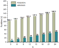
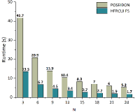
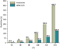
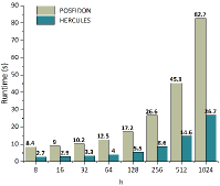
Figure 3: Running time of one training epoch. (a) Increase the number of users $N$ when the number of samples for each user is $|D_{i}|=200$. (b) Increase the number of users $N$ when the total sample size is $|D|=2000$. (c) Increase the total sample size $|D|$ when $N=10$. (d) Increase the sample dimension when $N=10$ and $|D|=200\times N$.

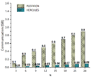
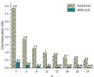
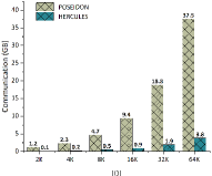
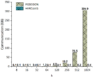
Figure 4: Evaluation of communication overhead for one training epoch. (a) Increase the number of users $N$ when given $|D_{i}|=200$ for each user $i$. (b) Increase the number of users $N$ when the total sample size $|D|=2000$. (c) Increase the total sample size $|D|$ when given $N=10$. (d) Increase the dimension of a single sample when given $N=10$ and $|D|=200\times N$.

We further analyze the scalability of Hercules and POSEIDON in terms of the number of users $N$, the number of samples $|D|$, and the number of dimensions $h$ for one sample. Here we use a two-layer architecture with 64 neurons in each layer. The local batch size for each user is 10. Figure 3 shows the experimental results, where we record the execution time of one training epoch, i.e., all the data of each user are processed once. Specifically, Figure 3 shows the execution time as the number of users grows, where we fix the number of samples held by each user as 200, and the dimension of each sample as 64. We can observe that the execution time of Hercules and POSEIDON shows a slight linear increase with the increase of the number of users. This stems from the fact that most of the operations performed by each user are concentrated locally except for the distributed bootstrapping procedure. Obviously, the percentage of $\mathbf{DBootstrap}$ operations over the total operations under ciphertext training is relatively small. We further fix the total number of samples in the system as 2000, and calculate the execution time of each user as the number of users increases. As shown in Figure 3, this causes a linear decrease in execution time since the increase in user data reduces the sample volume held by each user. Given the fixed number of users $N=10$ and $h=64$, Figure 3 shows that the execution time of each user increases linearly as $|D|$ increases. It is obvious that the increase in $|D|$ implies an increase in the number of samples in each user. Figure 3 also shows similar results under different sample dimensions.

In general, Hercules and POSEIDON show similar relationships in terms of computation cost under different hyper-parameters. However, we can observe that the running time of Hercules is far less than that of POSEIDON, due to the superiority of our new matrix multiplication method.

6.4 Communication Overhead

Tables III and IV show the total communication overhead required by Hercules and POSEIDON over different datasets. We can observe that during the training process, the ciphertext data that each user needs to exchange with other parties in Hercules are much smaller than that of POSEIDON. This also stems from the superiority of the new matrix multiplication method we design. Specifically, In POSEIDON, AP is used for matrix multiplication to achieve fast SIMD operations. However, as shown in the fourth row of Protocol 3 in [12], this method requires multiple copies and zero padding operations for each row or column of the input matrix, depending on the number of neurons in each hidden layer, the absolute value of the difference between the row or column dimension of the matrix and the number of neurons in the corresponding hidden layer. In fact, AP is an encoding method that trades redundancy in storage for computation acceleration. On the contrary, our method does not require additional element copy except for a small amount of zero padding in the initial stage to facilitate calculations. Therefore, Hercules obviously exhibits smaller communication overhead. For example, given the MNIST dataset, a 3-layer fully connected model with 64 neurons per layer, the communication overhead of each user in POSEIDON is about 703(GB) to complete 1000 global iterations, while Hercules only needs 17.58(GB) per user.

We also analyze the scalability of Hercules and POSEIDON in terms of the number of users $N$, the number of samples $|D|$, and the sample dimension $h$. Here we use a two-layer model architecture with 64 neurons in each layer. The local batch size for each user is 10. Figure 4 shows the experimental results. Similar to the results for computation cost comparison, we can observe that Hercules exhibits better scalability compared to POSEIDON under different hyper-parameters. In addition, we also show the storage overhead advantage of Hercules compared to POSEIDON, and discuss the performance of Hercules compared with other advanced MPC-based solutions. More details can be found in Table IX and Table VII in Appendix.

7 Conclusion

In this paper, we propose Hercules for privacy-preserving FL. We design a novel matrix coding technique to accelerate the training performance under ciphertext. Then, we use a novel approximation strategy to improve the compatibility of Hercules for processing non-polynomial functions. Experiments on benchmark datasets demonstrate the superiority of Hercules compared with existing works. In the future, we will focus on designing more efficient optimization strategies to further reduce the computation overhead of Hercules, to make it more suitable for practical applications.

Appendix

Appendix A Security Extensions

A.1 Active Adversaries

In Hercules, we consider a passive-adversary model with collusion of up to $N-1$ users. However, our work can also be extended to models in the presence of active adversaries. This can be achieved through verifiable computing techniques including zero-knowledge proofs (ZKF) [51] and redundant computation [11]. An intuitive idea is to use ZKF to ensure the format correctness of the ciphertext sent by the adversary, and use redundant calculations such as SPDZ [52] to verify the integrity of each party’s calculation results. This would come at the cost of an increase in the computation complexity, that will be analyzed as future work.

A.2 Out-of-the-Scope Attacks

The goal of Hercules is to protect the privacy of users’ local data and model parameters. However, there are still some attacks that can be launched from the prediction results of the model, e.g., membership inference [53], model inversion [54], or model stealing [55]. These attacks can be mitigated by complementary countermeasures that are also easily integrated into Hercules. For example, to defense the membership inference attack, on can add a carefully crafted noise vector to a confidence score vector to turn it into an adversarial example that misleads the attacker’s classifier [56]. We can also limit the number of prediction queries for the queriers, thereby reducing the risk of adversaries launching model stealing attacks [55]. We leave the combination of HE-based methods with existing defenses against various types of attacks as future works.

Appendix B The Baby-Step/giant-Step Algorithm Used in Algorithm 3

Given an integer $k\in(-h,h)$, we can rewrite $k=\sqrt{h}\cdot i+j$ where $-\sqrt{h}<i<\sqrt{h}$ and $0\leq j<\sqrt{h}$. Therefore, Eq.(9) can be parsed as

$$\begin{split}U^{\mu}\cdot\mathbf{a}&=\sum_{-\sqrt{h}<i<\sqrt{h},0\leq j<\sqrt{h}}(\mathbf{u}_{\sqrt{h}\cdot i+j}^{\mu}\odot\mathbf{R}(\mathbf{a},\sqrt{h}\cdot i+j))\\ &=\sum_{-\sqrt{h}<i<\sqrt{h}}\mathbf{R}(\sum_{0\leq j<\sqrt{h}}\mathbf{a}_{i,j},\sqrt{h}\cdot i)\end{split}$$

where $\mathbf{a}_{i,j}=\mathbf{R}(\mathbf{u}^{\mu}_{\sqrt{h}\cdot i+j},-\sqrt{h}\cdot i)\odot\mathbf{R}(\mathbf{a},j)$. Based on this, we can first compute $\mathbf{R}(\mathbf{a},j)$ for $0\leq j<\sqrt{h}$, and then use them to compute the encryption of $\mathbf{a}_{i,j}$. In general, Step 1-1 requires homomorphic operations of $2h$ additions, $2h$ constant multiplications, and $3\sqrt{h}$ rotations. Similarly, Step 1-2 can be completed by $h$ additions, $h$ constant multiplications, and $2\sqrt{h}$ rotations.

The number of constant multiplications required in Step 2 can also be reduced by exploiting two-input multiplexers. We can observe that

$$\begin{split}&\mathbf{Mul}_{pt}(\mathbf{Rot}([\mathbf{A}^{(0)}]_{pk},k-h),\mathbf{v}_{k-h})\\ &=\mathbf{Rot}(\mathbf{Mul}_{pt}([\mathbf{A}^{(0)}]_{pk},\mathbf{R}(\mathbf{v}_{k-h},h-k)),k-h)\\ &=\mathbf{Rot}([\mathbf{A}^{(0)}]_{pk}-\mathbf{Mul}_{pt}([\mathbf{A}^{(0)}]_{pk},\mathbf{R}(\mathbf{v}_{k},-k)),k-h)\end{split}$$

Then, we can first compute $\mathbf{Mul}_{pt}([\mathbf{A}^{(0)}]_{pk},\mathbf{R}(\mathbf{v}_{k},-k))$ for each $1\leq k<h$. Based on the fact that

$$\begin{split}\mathbf{Mul}_{pt}(\mathbf{Rot}([\mathbf{A}^{(0)}]_{pk},k),\mathbf{v}_{k})=\mathbf{Rot}(\mathbf{Mul}_{pt}([\mathbf{A}^{(0)}]_{pk},\mathbf{R}(\mathbf{v}_{k},-k)),k)\end{split}$$

we can get the ciphertext $[\mathbf{A}^{(k)}]_{pk}$ with addition and rotation operations.

Appendix C Matrix Transposition on Packed Ciphertexts

In this section, we introduce how to homomorphically transpose a matrix under the packed ciphertext. Let $\mathbf{a}=\iota^{-1}(A)\in R^{n}$ indicate the vector representation of a matrix $A$, $U^{T}$ is defined as the matrix representation of the transpose map $A\mapsto A^{T}$ on $R^{h\times h}\cong R^{n}$. Then, for $0\leq i,j<h$, each element in $U^{T}$ can be expressed as

$${U}_{h\cdot i+j,k}^{T}=\left\{\begin{aligned} &1\quad\mathsf{if}\;k=h\cdot j+i;\\ &0\quad\mathsf{otherwise}.\\ \end{aligned}\right.$$

Hence, the $k$-th diagonal vector of $U^{T}$ is nonzero if and only if $k=(h-1)\cdot i$ for some $i\in\mathbb{Z}\cap(-h,h)$. As a result, $U^{T}$ has a total of $(2h-1)$ nonzero diagonal vectors as a sparse matrix. Therefore, linear transformation for matrix transpose can be expressed as

$$\begin{split}U^{T}\cdot\mathbf{a}=\sum_{-h<i<h}(\mathbf{t}_{(h-1)\cdot i}\odot\mathbf{R}(\mathbf{a},(h-1)\cdot i))\end{split}$$ (18)

where we use $\mathbf{t}_{(h-1)\cdot i}$ to represent the nonzero diagonal vector of $U^{T}$. When $i\geq 0$, the $t$-th component of the vector $\mathbf{t}_{(h-1)\cdot i}$ is computed by

$$\mathbf{t}_{(h-1)\cdot i}[t]=\left\{\begin{aligned} &1\quad\mathsf{if}\;t-i=(h+1)\cdot j,0\leq j<h-i;\\ &0\quad\mathsf{otherwise}.\\ \end{aligned}\right.$$

If $i\leq 0$, we have

$$\mathbf{t}_{(h-1)\cdot i}[t]=\left\{\begin{aligned} &1\quad\mathsf{if}\;t+i=(h+1)\cdot j,0\leq j<h+i;\\ &0\quad\mathsf{otherwise}.\\ \end{aligned}\right.$$

In general, the computation cost required for matrix transposition is about $2h$ rotations, which can be further reduced to $3\sqrt{h}$ by the previously described baby-step/giant-step method.

Appendix D Rectangular Matrix Multiplication on Packed Ciphertexts

We extend the homomorphic multiplication between square matrices to general rectangular matrices, such as $R^{t\times h}\times R^{h\times h}\rightarrow R^{t\times h}$ or $R^{h\times h}\times R^{h\times t}\rightarrow R^{h\times t}$. Without loss of generality, we consider $t<h$. For a $(h_{1}\times h)$-dimensional matrix $A_{1}$ and a $(h_{2}\times h)$-dimensional matrix $A_{2}$, we use $(A_{1};A_{2})$ to represent the $(h_{1}+h_{2})\times h$ matrix which is obtained by concatenating $A_{1}$ and $A_{2}$ in a vertical direction. Similarly, $(A_{1}|A_{2})$ indicates the matrix concatenated in a horizontal direction if matrices $A_{1}$ and $A_{2}$ have the same number of rows.

A naive solution to perform multiplication between rectangular matrices is to convert any matrix into a square matrix through zero padding, and then use Algorithm 3 to implement the multiplication between square matrices homomorphically. This leads to a rotation with a complexity of $O(h)$. We provide an improved method through insight into the property of matrix permutation.
Refined Rectangular Matrix Multiplication. Given a $t\times h$ matrix $A$ and an $h\times h$ matrix $B$ with $t$ divide $h$, we introduce a new symbol $C_{t_{1}:t_{2}}$, which is denoted the $(t_{2}-t_{1})\times h$ submatrix of $C$ formed by extracting from $t_{1}$-th row to the $(t_{2}-1)$-th row of $C$. As a result, the product of $AB$ can be expressed as below.

$$\begin{split}A\cdot B&=\sum_{k=0}^{h-1}(\phi^{k}\circ\mu(A))\odot\left((\pi^{k}\circ\zeta(B))_{0:t}\right)\\ &=\sum_{0\leq i<t}\sum_{0\leq j<h/t}(\phi^{j\cdot t+i}\circ\mu(A))\odot\left((\pi^{j\cdot t+i}\circ\zeta(B))_{0:t}\right)\end{split}$$ (19)

Our key observation is the following lemma, which provides us with ideas for designing fast rectangular matrix multiplication.

Lemma D.1.

Permutation $\phi$ and $\mu$ are commutative. For $k>0$, we have $\phi^{k}\circ\mu=\mu\circ\phi^{k}$. Also, $\pi^{k}\circ\zeta=\zeta\circ\pi^{k}$ for $k>0$.

Based on Lemma D.1, we define an $h\times h$-dimensional matrix $\tilde{A}$, which contains $h/t$ copies of $A$ from the vertical direction (i.e., $\tilde{A}=(A;\cdots;A)$). It means that

$$\begin{split}(\phi^{i}\circ\mu(\tilde{A}))_{j\cdot t:(j+1)\cdot t}&=(\phi^{i}\circ\mu(\tilde{A})_{j\cdot t:(j+1)\cdot t})\\ &=\phi^{i}\circ\mu\circ\phi^{j\cdot t}(A)\\ &=\phi^{j\cdot t+i}\circ\mu(A)\end{split}$$ (20)

Then, we can further compute

$$\begin{split}(\pi^{i}\circ\zeta({B}))_{j\cdot t:(j+1)\cdot t}=(\pi^{j\cdot t+i}\circ\zeta(B))_{0:t}\end{split}$$ (21)

As a result, the matrix product $AB$ can be rewritten as below.

$$\begin{split}A\cdot B=\sum_{0\leq j<h/t}\left(\sum_{0\leq i<t}(\phi^{i}\circ\mu(\tilde{A}))\odot(\pi^{i}\circ\zeta({B}))\right)_{j\cdot t:(j+1)\cdot t}\end{split}$$

Homomorphic Rectangular Matrix Multiplication. Given two ciphertexts $[\mathbf{\tilde{A}}]_{pk}$ and $[\mathbf{{B}}]_{pk}$, we can first compute $\mu{(\tilde{A})}$ and $\zeta({B})$ utilizing the baay-step/giant-step approach. Then, $\sum_{0\leq i<t}(\phi^{i}\circ\mu(\tilde{A}))\odot(\pi^{i}\circ\zeta({B}))$ can be securely computed in a similar way to Algorithm 3. Finally, we get the encryption of ${A}B$ by performing aggregation and rotations operations. The details are shown in Algorithm V.

Algorithm 6 Homomorphic Rectangular Matrix Multiplication

0:  HE-RMatMult $([\mathbf{\tilde{A}}]_{pk},[\mathbf{B}]_{pk})$

1:  $[\mathbf{A}^{(0)}]_{pk}\leftarrow$ HE-LinTrans $([\mathbf{\tilde{A}}]_{pk},U^{\mu})$

2:  $[\mathbf{B}^{(0)}]_{pk}\leftarrow$ HE-LinTrans $([\mathbf{A}]_{pk},U^{\zeta})$

3:  for $k=1$ to $t-1$ do

4:     $[\mathbf{A}^{(k)}]_{pk}\leftarrow$ HE-LinTrans $([\mathbf{A}^{(0)}]_{pk},V^{k})$

5:     $[\mathbf{B}^{(k)}]_{pk}\leftarrow$ HE-LinTrans $([\mathbf{B}^{(0)}]_{pk},P^{k})$

6:  end for

7:  $[\mathbf{\tilde{A}B}]_{pk}\leftarrow\mathbf{Mul}_{ct}([\mathbf{A}^{(0)}]_{pk},[\mathbf{B}^{(0)}]_{pk})$

8:  for $k=1$ to $t-1$ do

9:     $[\mathbf{\tilde{A}B}]_{pk}\leftarrow\mathbf{Add}([\mathbf{\tilde{A}B}]_{pk},\mathbf{Mul}_{ct}([\mathbf{A}^{(k)}]_{pk},[\mathbf{B}^{(k)}]_{pk}))$

10:  end for

11:  $[\mathbf{AB}]_{pk}\leftarrow[\mathbf{\tilde{A}B}]_{pk}$

12:  for $k=0$ to $\log(h/t)-1$ do

13:     $[\mathbf{AB}]_{pk}\leftarrow\mathbf{Add}([\mathbf{{A}B}]_{pk},\mathbf{Rot}([\mathbf{{A}B}]_{pk},t\cdot h\cdot 2^{k}))$

14:  end for

15:  return $[\mathbf{AB}]_{pk}$

TABLE V: Complexity of Algorithm 6

Step	$Add$	$mul_{pt}$	$Rot$	$mul_{ct}$
1	$3h$	$3h$	$5\sqrt{h}$	-
2	$t$	$2t$	$3t$	-
3	$t$	-	-	$t$
4	$\log(h/t)$	-	$\log(h/t)$	-
Total	$3h+2t$	$4h$	$3h+5\sqrt{h}$	$t$

Table V presents the total complexity of Algorithm 6. We observe that compared with Algorithm 3, it reduces the complexity of the rotation operations of steps 2 and 3 to $O(t)$, although additional operation is required for step 4. Moreover, the final result $[\mathbf{AB}]_{pk}$ is a ciphertext of a $h\times h$-dimensional matrix containing $(h/t)$ copies of the expected matrix product $AB$ in a vertical direction. Hence, the resulting ciphertext remains the format as a rectangular matrix, and it can be further performed matrix calculations without additional overhead.

Appendix E Parallel Matrix Computation

The above matrix operations are all performed in the message space $R^{n}$, where we assume that $n=h^{2}$. Actually, most HE schemes have a lot of plaintext slots (up to thousands) compared to the dimension of the matrix in deep learning, that is, usually $n\gg h^{2}$. Hence, most plaintext slots will be wasted if a ciphertext is only used to store a matrix. We provide a method of encrypting multiple matrices into a ciphertext, so as to realize parallel matrix calculation in a SIMD manner. Specifically, we assume that $n$ is divisible by $h$ and let $\beta=n/h^{2}$. Then the encoding map described in above for singe matrix will be modified as $\iota_{\beta}:R^{n}\rightarrow(R^{h\times h})^{\beta}$. For an input vector $\mathbf{a}=(a_{t})_{0\leq t<n}$, $\iota_{\beta}$ is defined as below.

$$\begin{split}\iota_{\beta}:\mathbf{a}\mapsto\left(A_{k}=(a_{\beta(h\cdot i+j)+k})\right)_{0\leq k<\beta}.\end{split}$$ (22)

The components of $\mathbf{a}$ with indexes congruent to $k$ modulo $\beta$ are corresponding to the $k$-th matrix $A_{k}$. We observe that for an integer $0\leq t<h^{2}$, the rotation operation $\mathbf{R}(\mathbf{a},\beta t)$ represents the matrix-wise rotation by $\beta$ positions. This can be naturally extended to other operations including scalar linear conversion and matrix multiplication. For example, when a single ciphertext is embedded in $\beta$ ($h\times h$)-dimensional matrices, we can immediately perform matrix multiplication between $\beta$ pairs matrices by using the previously described algorithm on two ciphertexts. This total computation complexity is consistent with Algorithm 3, but results in a less amortized computation complexity of $O(h/\beta)$ for each matrix.

Appendix F Proof of Lemma  4.1

Proof (Sketch).

We use induction to prove it. First, it is true for n=1. Assume that $p_{d}=\frac{2d+1}{4^{d}}\begin{pmatrix}2d\\ d\end{pmatrix}$ for some $d\leq 1$, Hence, we have

$$\begin{split}p_{d+1}&=p_{d}+\frac{1}{4^{d+1}}\begin{pmatrix}2d+2\\ d+1\end{pmatrix}\\ &=\frac{1}{4^{d+1}}\left(\frac{2(2d+2)!}{(d+1)!d!}+\frac{(2d+2)!}{(d+1)!(d+1)!}\right)\\ &=\frac{2d+3}{4^{d+1}}\begin{pmatrix}2d+2\\ d+1\end{pmatrix}\end{split}$$

Hence, the lemma is proved by induction. ∎

Appendix G Proof of Lemma  4.2

Proof (Sketch).

Obviously, $g_{d}(m)\leq g_{d}(1)=1$ for $m\in[0,1]$. We define $G(m)=(1-m)^{p_{d}}-(1-g_{d}(m))$, and then we prove that $G(m)\geq 0$ for $m\in[0,1]$ by showing
1. $G(0)=G(1)=0$.
2. there exists $m_{0}\in(0,1)$ s.t. $G(m_{0})>0$.
3. there exists a unique $y_{0}\in(0,1)$ s.t. $G^{\prime}(y_{0})=0$.

We first explain that the above three conditions are derived from $G(m)\geq 0$. Specifically, if there is a point $m\in(0,1)$ such that $G(m_{1})<0$, then according to the continuity of $G$, there is a root $m_{2}$ of the function $G$ between $m_{0}$ and $m_{1}$. From the mean value theorem, it is obvious that there exist $y_{1}\in(0,m_{2})$ and $y_{2}\in(x_{2},1)$ satisfying $G^{\prime}(y_{1})=G^{\prime}(y_{2})=0$, which contradicts the third condition. We begin to prove these three conditions. The first one is trivial. For the second condition, we observe that $G(0)=0$, $G^{\prime}(0)=0$ and $G^{\prime\prime}(0)>0$. We can infer that $G^{\prime}(m)>0$ for $m\in(0,\epsilon)$ for some $\epsilon>0$, based on the continuity of $G^{\prime\prime}$. Further, since $G(0)=0$, we have $G(m)>0$ for $m\in(0,\epsilon)$ which implies the second condition.

To prove uniqueness, let $G^{\prime}(m)=p_{d}(1-m^{2})^{d}-p_{d}(1-m)^{p_{d}-1}=0$. Then we have $(1-m)^{d-p_{d}+1}\cdot(1+m)^{d}=1$ for $m\in(0,1)$. Logarithmically, it holds that

$$\begin{split}\frac{\log(1+m)}{\log(1-m)}=-\frac{d-p_{d}+1}{d}\end{split}$$

Since $\frac{\log(1+m)}{\log(1-m)}$ is a strictly increasing function, this is the unique $y_{0}\in(0,1)$ that satisfies $G^{\prime}(y_{0})=0$. ∎

Appendix H Proof of Lemma  4.3

Proof (Sketch).

Let $y=1-m$, and define

$$\begin{split}H(y)=\frac{p_{d}\cdot 2^{d}}{d+1}\cdot y^{d+1}-(1-g_{d}(1-y))\end{split}$$

Then $H(y)^{\prime}=p_{d}\cdot 2^{d}\cdot y^{d}-g_{d}^{\prime}(1-y)=p_{d}\cdot 2^{d}\cdot y^{d}-p_{d}\cdot y^{d}(2-y)^{d}\geq 0$ for $y\in[0,1]$. Based on $H(0)=0$, it holds that $H(y)\geq 0$. Hence, for $m\in[0,1]$, we have

$$\begin{split}1-g_{d}(m)\leq\frac{p_{d}\cdot 2^{n}}{d+1}\cdot(1-m)^{d+1}\leq 2^{d}\cdot(1-m)^{d+1}\end{split}$$

∎

Appendix I Experimental comparisons with work [34]

TABLE VI: Comparisons with work [34]

$\sigma$	Work [34]	Ours
$8$	$208$ s ($50.78$ ms)	$21$ s ($5.12$ ms)
$10$	$307$ s ($74.9$ ms)	$27$ s ($6.59$ ms)
$12$	$532$ s ($129.8$ ms)	$37$ s ($9.03$ ms)
$14$	$823$ s ($200.9$ ms)	$51$ s ($12.45$ ms)
$16$	$1392$ s ($339.8$ ms)	$70$ s ($17.08$ ms)
$18$	$1930$ s ($471.11$ ms)	$76$ s ($18.5$ ms)
$20$	$2740$ s ($668.9$ ms)	$84$ s ($20.05$ ms)

TABLE VI shows the running times of work [34] and our method for approximation of the sign function, where $\delta$ is used to represent the error bound, i.e., $2^{-\sigma}$ means that the value error of the original function and the approximated function is small than $2^{-\sigma}$, $\mathcal{N}=2^{14}$ and $Q_{\mathcal{L}}=2^{2250}$. We observe that the running time of our method is much smaller than that of [34]. For example, the amortized running time of [34] to obtain the approximate result of sign function within $2^{-20}$ errors is 668.9 milliseconds (amortized running time), while the running time of our method is only 20.05 milliseconds, which is $33$ times faster than [34].

Appendix J Details Implementation of Hercules

Figure 5 presents the details of implementing Hercules, which essentially executes Algorithm 1 under the ciphertext. Note that we assume that all matrices involved in training have the same dimensions for simplicity. In actual implementation, the user can adaptively select the dimension so as to use Algorithm  3 or 6 to obtain the ciphertext result. $\mathbf{RS}(\cdot)$ is used to resulting ciphertext after each multiplication. This means that for the ciphertext with an initial layer number of $\mathcal{L}$, the maximum depth of $\mathcal{L}$ ciphertext multiplication can be evaluated. In practical applications, assuming $Q_{\mathcal{L}}/\Delta=r$, the ciphertext can be rescaled after $r$ multiplications instead of after each multiplication. On the other hand, Figure 5 only requires each user to perform the distributed bootstrapping function (i.e., $\mathbf{DBootstrap}$) when calculating the activation function, because this process usually requires more circuit depth. Similarly, in practice, users can adaptively execute $\mathbf{DBootstrap}$ as long as the depth of the circuit is about to be exhausted.

Implementation of Hercules

• Prepare: - This process is exactly the same as described in Algorithm 5. For $k=0$ to $k=H-1$, $\mathcal{C}$ and all users perform the following operations in concert. • Feedforward: - Each user ${P}_{i}$ computes $\hat{X_{i}}$, $\hat{Y_{i}}$ by the function $\mathbf{Ecd}(\cdot)$ and encrypts them as $[\mathbf{X_{i}}]_{pk}$ and $[\mathbf{Y_{i}}]_{pk}$. For $j=1$ to $j=\mathbb{L}$, each user ${P}_{i}$ performs following operations. - Compute $[\mathbf{E_{j,i}^{k}}]_{pk}=$HE-MatMult $(\mathbf{[\omega_{j}^{k}}]_{pk},[\mathbf{M_{j-1,i}^{k}}]_{pk})$, where $E_{j,i}^{k}={\omega}_{j}^{k}\times M_{j-1,i}^{k}$, $\mathbf{RS}([\mathbf{E_{j,i}^{k}}]_{pk})$. - Compute $[\mathbf{M_{j,i}^{k}}]_{pk}$, where $M_{j,i}^{k}={\varphi(E_{j,i}^{k})}$, $\mathbf{RS}([\mathbf{M_{j,i}^{k}}]_{pk})$. $\varphi(\cdot)$ is approximated as a polynomial in advance. - All users collaboratively compute $\mathbf{DBootstrap}([\mathbf{M_{j,i}^{k}}]_{pk},\mathcal{L}_{[\mathbf{M_{j,i}^{k}}]_{pk}},\Delta_{[\mathbf{M_{j,i}^{k}}]_{pk}},\{sk_{i}\})$. • Backpropagation: - Each $P_{i}$ computes $[\mathbf{L_{\mathbb{L},i}^{k}}^{\prime}]_{pk}=\mathbf{Sub}([\mathbf{Y_{i}}]_{pk},\mathbf{[M_{\mathbb{L},i}^{k}}]_{pk})$, $[\mathbf{L_{\mathbb{L},i}^{k}}]_{pk}=\mathbf{Mul}_{ct}([L_{\mathbb{L},i}^{k}]_{pk},[L_{\mathbb{L},i}^{k}]_{pk})$, where $L_{\mathbb{L}}^{k}=||y[t]-M_{\mathbb{L}}^{k}||_{2}$. - Each $P_{i}$ computes $[\mathbf{L_{\mathbb{L},i}^{k}}]_{pk}$ with basic SIMD operations, where $L_{\mathbb{L}}^{k}=\varphi^{\prime}(E_{\mathbb{L}}^{k})\odot L_{\mathbb{L}}^{k}$. Then, computes $\mathbf{RS}([\mathbf{L_{\mathbb{L},i}^{k}}]_{pk})$. - Each $P_{i}$ computes $[\mathbf{(M_{\mathbb{L}-1,i}^{k})}^{T}]_{pk}=\texttt{HE-LinTrans}({\mathbf{[M_{\mathbb{L}-1,i}^{k}]}_{pk}},U^{(\mathbb{L}-1)})$, where $U^{(\mathbb{L}-1)}$ is the permutation representation matrix of ${(\mathbf{M_{\mathbb{L}-1,i}^{k})}}^{T}$. - Each $P_{i}$ computes $[\bigtriangledown\mathbf{{\omega}_{\mathbb{L},i}^{k}}^{\prime}]_{pk}=$HE-MatMult $([\mathbf{(M_{\mathbb{L}-1,i}^{k})}^{T}]_{pk},[\mathbf{{L}_{\mathbb{L},i}^{k}}]_{pk})$. Then, computes $\mathbf{RS}([\bigtriangledown\mathbf{{\omega}_{\mathbb{L},i}^{k}}^{\prime}]_{pk})$. - Each $P_{i}$ computes $[\bigtriangledown\mathbf{{\omega}_{\mathbb{L},i}^{k}}]_{pk}=\mathbf{Add}([\bigtriangledown\mathbf{{\omega}_{\mathbb{L},i}^{k}}^{\prime}]_{pk},\mathbf{[\bigtriangledown\mathbf{{\omega}_{\mathbb{L},i}^{k}}]}_{pk})$, and $\mathbf{RS}([\bigtriangledown\mathbf{{\omega}_{\mathbb{L},i}^{k}}]_{pk})$, where $\bigtriangledown{\omega}_{\mathbb{L},i}^{k}=\bigtriangledown{{\omega}_{\mathbb{L},i}^{k}}+{(M_{\mathbb{L}-1,i}^{k})}^{T}\times{L_{\mathbb{L},i}^{k}}$. For $j=\mathbb{L}-1$ to $j=1$, each user ${P}_{i}$ performs following operations. - Compute $[\mathbf{\omega_{j+1,i}^{k})}^{T}]_{pk}=\texttt{HE-LinTrans}([\mathbf{\omega_{j+1,i}^{k})}]_{pk},U^{(\mathbb{L}-1)})$, where $U^{(j+1)})$ is the permutation representation matrix of $(\omega_{j+1,i}^{k})^{T}$. - Compute $[\mathbf{L_{j}^{k}}]_{pk}=$HE-MatMult $([\mathbf{L_{j+1}^{k}}]_{pk},[\mathbf{\omega_{j+1,i}^{k}}^{T}]_{pk})$.Then, computes $\mathbf{RS}([\mathbf{L_{j}^{k}}]_{pk})$, where $L_{j}^{k}=L_{j+1}^{k}\times(\omega_{j+1}^{k})^{T}$. - Compute $[\mathbf{L_{j,i}^{k}}]_{pk}$ with basic SIMD operations, where $L_{j,i}^{k}=\varphi^{\prime}(E_{l,i}^{k})\odot L_{j,i}^{k}$. Then, computes $\mathbf{RS}([\mathbf{L_{j,i}^{k}}]_{pk})$. - Compute $[\bigtriangledown\mathbf{{\omega}_{j,i}^{k}}^{\prime}]_{pk}=$HE-MatMult $([\mathbf{(M_{j-1,i}^{k})}^{T}]_{pk},[\mathbf{L}_{j,i}^{k}]_{pk})$. Then, computes $\mathbf{RS}([\bigtriangledown\mathbf{{\omega}_{j,i}^{k}}^{\prime}]_{pk})$. - Compute $[\bigtriangledown\mathbf{{\omega}_{j,i}^{k}}]_{pk}=\mathbf{Add}([\bigtriangledown\mathbf{{\omega}_{j,i}^{k}}^{\prime}]_{pk},\mathbf{[\bigtriangledown\mathbf{{\omega}_{j,i}^{k}}]}_{pk})$, and $\mathbf{RS}([\bigtriangledown\mathbf{{\omega}_{j,i}^{k}}]_{pk})$, where $\bigtriangledown{\omega}_{j,i}^{k}=\bigtriangledown{{\omega}_{j,i}^{k}}+{(M_{j-1,i}^{k})}^{T}\times{L_{j,i}^{k}}$. • Aggregation: For $j=1$ to $j=\mathbb{L}$, the cloud server $\mathcal{C}$ performs following operations. - Compute $[\mathbf{{\bigtriangledown\omega}_{j}^{k}}]_{pk}=[\sum_{i=1}^{N}\mathbf{\bigtriangledown{\omega}_{j,i}^{k}}]_{pk}$ with the basic $\mathbf{Add}$ function. - Compute $[\mathbf{{\omega}_{j}^{k+1}}^{\prime}]_{pk}=\mathbf{Mul}_{pt}([\mathbf{\bigtriangledown{\omega}_{j}^{k}}]_{pk},\frac{\eta}{\mathcal{B}\times N})$. - Compute $[\mathbf{{\omega}_{j}^{k+1}}]_{pk}=\mathbf{Sub}([\mathbf{{\omega}_{j}^{k}}]_{pk},[\mathbf{{\omega}_{j}^{k+1}}^{\prime}]_{pk})$ and broadcasts them to all users, where ${\omega}_{j}^{k+1}={\omega}_{j}^{k}-\frac{\eta}{\mathcal{B}\times N}\bigtriangledown{\omega}_{j}^{k}$.

Fig. 5: Detailed description of Hercules

Appendix K Datasets Used in Experiments

Consistent with POSEIDON [12], we choose the following public datasets in our experiments.

• The Breast Cancer Wisconsin dataset (BCW) [45], which has a total of $|D|=699$ samples, and the dimension of each sample is $h=9$, with $\omega_{\mathbb{L}}=2$, where $\omega_{\mathbb{L}}$ represents the number of labels (also the number of neurons in the last layer of the neural network (NN)).

• MNIST dataset [46] with $|D|=70,000$, $h=28\times 28$, and $\omega_{\mathbb{L}}=10$.

• The Epileptic seizure recognition (ESR) dataset [47] with $|D|=11,500$, $h=179$, and $\omega_{\mathbb{L}}=2$.

• The default of credit card clients (CREDIT) [48] with $|D|=30,000$, $h=23$, and $\omega_{\mathbb{L}}=2$.

• The street view house numbers (SVHN) dataset [49] with colored images (3 channels), with $|D|=600,000$, $h=3\times 32\times 32$, and $\omega_{\mathbb{L}}=10$.

• CIFAR-10 and CIFAR-100 with $|D|=60,500$, $h=3\times 32\times 32$, $\omega_{\mathbb{L}}=10$, and $\omega_{\mathbb{L}}=100$, respectively.

We convert SVHN to gray-scale to reduce the number of channels. In addition, we make the dimension of each weight matrix to the nearest power of 2 by padding zeros. As a result, we actually train the NN on the CREDIT, ESR, and MNIST datasets with the feature dimensions of 32, 256, 1024, respectively. Since SVHN is grayed out, the dimension of its features already meets the power of 2. On the other hand, we generate synthetic data to evaluate the scalability of the system, where we record the system performance under different features or the number of samples. For simplicity, we uniformly and randomly distribute all the above datasets to users. Note that the distribution of data among different users may affect the accuracy of the model, but this is orthogonal to the focus of this paper. Since Hercules is designed for general federated learning scenario, all existing processing strategies for data distribution can be seamlessly integrated into Hercules.

TABLE VII: Comparison with existing MPC-based works

	ABY2.0	Trident	SWIFT	CRYPTFLOW	XONN	BLAZE	ABY3	SecureML	GALA	Hercules
	[19]	[23]	[57]	[21]	[58]	[22]	[8]	[20]	[28]
MPC Setup	2PC	4PC	3/4PC	3PC	2PC	3PC	3PC	2PC	2PC	N-party
Inference	✓	✓	✓	✓	✓	✓	✓	✓	✓	✓*
Training	✓	✓	✓	✗	✗	✗	✓	✓	✗	✓
Adversarial model	1 P	1 A/P	2 A/P	2 P	1P	1A	1 A/P	1P	1P	N-1P
Collusion	✗	✗	2	✗	✗	✗	✗	✗	✗	N-1
Techniques	GC, SS	GC, SS	SS	GC, SS	GC, SS	GC, SS	GC, SS	GC, SS	GC, HE	HE
Linear operation	✓	✓	✓	✓	✓	✓	✓	✓	✓	✓
Conv. operation	✓	✓	✓	✓	✓	✗	✓	✓	✓	✓
Pooling operation	✓	✓	✓	✓	✓	✗	✓	✓	✓	✓

• 2PC represents the secure multi-party computing protocol between the two parties, and the rest can be deduced by analogy. A/P means active or passive adversary. ✓* indicates that Hercules also supports N-party distributed inference, because inference can be seen as a sub-process of training.

Appendix L Neural Network Structure

We use the following NN structures to train specific datasets.

• We train a 2-layer fully connected NN with BCW, ESR and CREDIT data sets, where each layer contains $64$ neurons. Similarly, the same structure was used to test the cost of Hercules on the synthetic dataset.

• We train a three-layer fully connected NN with 64 neurons in each layer for the MNIST and SVHN datasets.

• We train two models for CIFAR-10 dataset. Specifically, (i) a CNN structure contains $2$ convolutional layers (CV), an average pooling layer, a max pooling layer with kernel size of $2\times 2$, and two fully connected layer (FC) which contains $128$ and $10$ neurons, respectively. We called this structure as CIFAR-10-N1. (ii) a CNN structure contains $4$ CV with kernel size of $3\times 4$, an average pooling layer and a max pooling layer with kernel size of $2\times 2$, and 2 FC which contain $128$ and $10$ neurons, respectively. We called this structure as CIFAR-10-N2.

• For CIFAR-100, we train a CNN structure consisting of $6$ CV with kernel size of $3\times 4$, an average pooling layer and a max pooling layer with kernel size of $2\times 2$, and 2 FC which contain $128$ neurons for each layer.

We changed the number of filters from 3 to 16 for all CV layers. The number of global iterations used to train the above models is 100; 500; 600; 1000; 18,000; 16,800; 25,000 and 54,000 for BCW, CREDIT, ESR, MNIST, SVHN, CIFAR-10-N2, CIFAR-10-N1, and CIFAR-100, respectively. The local batch size of each user is set to 10, thus the global batch size is 100 for 10 users, and 500 for 50 users.

Appendix M Learning Extensions

M.1 Asynchronous distributed learning with uneven data distribution

In Hercules, we rely on all users online to complete the global update of the gradient under the ciphertext. However, Hercules also supports asynchronous neural network learning, which can be realized by the server only receiving data from users within a certain threshold time. In this case, the training of the neural network mainly benefits from the local data of users with good network status. Noted that the smooth execution of the distributed bootstrapping operation $\mathbf{DBootstrap}$ requires the participation of all users. This operation instead of being done in a centralized manner usually requires more computation and communication overhead.

In Hercules, we evenly distribute the data to each user for the simplicity of the experiment. In fact, the uneven distribution of users’ data and asynchronous gradient descent will inevitably affect the accuracy of the model. How to deal with these problems has been extensively studied [59, 60], which are orthogonal to this work. Note that our privacy protection method is independent of the distribution of user data and the way of gradient update. Hence, all existing works can be seamlessly integrated into Hercules.

M.2 Training on Other Neural Networks

In this work, we focus on deploying Hercules on MLPs and CNNs, and demonstrate the performance of our packing scheme and function approximation method under these NNs. For other structures, such as long short-term memory (LSTM)[61], recurrent neural network (RNN)[62] and residual neural network (ResNet) [63], Hercules needs to modify the local gradient update process according to their forward and backward pass operations. For example, ResNet has skip connections to skip certain layers, so after skipping a layer, the shape of the encrypted ciphertext should be aligned according to the weight matrix to be multiplied. This can be ensured by using the rotation function of CKKS (rearrange the slots of the ciphertext). We believe that these modifications are not significant. Although POSEIDON is tailored for MLPs and CNNs, in essence, Hercules can be used to quickly calculate any mathematical operation under ciphertext, which constitutes the main body of other neural network structures.

Appendix N Microbenchmarks of Hercules and POSEIDON

TABLE VIII: Microbenchmarks of Hercules and POSEIDON

Functionality	Execution time (s)	Comm. (MB)
Approx_Sigmoid	0.017 — 0.017	–
Appro_ReLu	0.01 — 0.09	–
Appro_Softmax	0.07 — 0.07	–
Average-pooling	0.034—0.034	–
Max-pooling	5.73—1.91	23.5—6.9
DBootstrap	0.09 — 0.09	4.5 — 1.5
FC layer	0.097 — 0.0015	–
FC layer-backprop	0.14 — 0.002	–
CV layer	0.04 — 0.0006	–
CV layer-backprop	0.06 — 0.0009	–
DKeySwitch	0.06 — 0.06	22.14 — 22.14

We present the microbenchmark cost of Hercules and POSEIDON in performing different functions. As shown in Table VIII, the bold font represents the overhead of Hercules. For experimental configurations, We consider the number of users $N=10$, the dimension of each sample is $h=32$, the number of neurons in each layer is 64 or with kernel size $3\times 3$, and the dimension of cyclotomic polynomial ring used in CKKS is set $\mathcal{N}=2^{13}$. All the costs represent the processing of 1 sample per party.

We record the computation and communication costs (in an amortized way) of calculating FC, CV, FC backpropagation, CV backpropagation, and different activation functions in Hercules and POSEIDON. For the activation functions sigmoid and sofmax, Hercules and POSEIDON exhibit the same overhead because they both use the same function approximation method. For ReLU, since Hercules uses a 20 bit-precision composite polynomial to fit the original function, while POSEIDON simply uses a polynomial with a degree of 3 to approximate the original ReLU (using the least squares method), it makes the cost of Hercules larger than POSEIDON but derives a higher approximation accuracy. Note that given the same error bound, the time required to calculate the polynomial generated by the least square method under ciphertext is much longer than ours. For max pooling, POSEIDON replaces it with Chebyshev function interpolation, thereby obtaining a polynomial of degree 31 with a precision of 7 bits. Experimental results show that our 7-bit precision composite polynomial is much less expensive than POSEIDON. This is mainly due to the characteristics of composite polynomials. As discussed before, a composite function with degree of $deg(G)$ can be calculated with a complexity of $O(\log(deg(G)))$, while the computation complexity of calculating any function $G$ is at least $\Theta(\sqrt{deg(G)})$.

The operations in FC, CV and their backpropagation are mainly composed of matrix multiplication. As shown in Table VIII, Hercules is far superior to POSEIDON in terms of calculating homomorphic matrix multiplication. Specifically, POSEIDON adopts AP to achieve fast SIMD calculations. For the multiplication of two $h\times h$-dimensional matrices, the complexity of the homomorphic rotation operation required by AP is $\max_{i\in[\mathbb{L}]}(\omega_{i}\times\log(h\times\omega_{i}))$. For Hercules, as shown in Table I, the complexity required for the matrix multiplication is only $3h+5\sqrt{h}$. Moreover, AP requires multiple copies and zero padding operations for each row or column of the input matrix, (depending on the number of neurons in each hidden layer, and the absolute value of the difference between the row or column dimension of the matrix and the corresponding hidden layer neuron. On the contrary, our method does not require additional element copying except for a small amount of zero padding in the initial stage to facilitate calculations. Therefore, Hercules obviously exhibits lower communication overhead.

Appendix O Storage Overhead

TABLE IX: Comparison of storage cost

Datasets	Storage cost (GB)
	Hercules	POSEIDON
BCW	$0.0012$	0.095
ESR	$0.184$	$11.778$
CREDIT	$0.061$	$3.948$
MNIST	$4.906$	$314.025$
SVHN	$54.9$	$3515.6$
CIFAR-10	$16.47$	$2109.37$
CIFAR-100	$16.47$	$2109.37$

As shown in TABLE IX, we also count the storage overhead required for training each scheme on different datasets, where the storage overhead is mainly dominated by the size of the ciphertext that each user needs to save locally. We observe that the storage overhead required by Hercules on each dataset is much lower than that of POSEIDON. Since POSEIDON designs a alternating packing (AP) method to pack ciphertext in the encryption process, this leads to multiple copies and zero padding operations for each ciphertext, depending on the number of neurons in each hidden layer. On the contrary, our method does not require additional element copying except for a small amount of zero padding in the initial stage to facilitate calculations.

Appendix P Comparison with Other Prior Works

Beyond the HE-based schemes, a wealth of MPC solutions based on interaction between multiple servers have been proposed to design privacy-preserving neural network training and prediction frameworks. These solutions may be not practical in the real-world setting without multiple servers. Nevertheless, we still make a rough comparison between these works and Hercules to demonstrate the merits and demerits of each scheme. As shown in Table VII in the Appendix, MPC protocol with multiple servers relies on splitting the training task into two or more servers, where the servers are usually assumed to be non-colluding. Then, the state-of-the-art secret sharing methods, including arithmetic sharing [19], boolean sharing [8], and Yao’s garbled circuit [21] are carefully integrated to efficiently implement various mathematical operations under the ciphertext. It is computationally cost-effective, avoiding the high communication overhead among large-scale users. For example, given the MNIST dataset, we roughly compare the computational cost of Hercules, ABY³ [8], and XONN [58] in training the same network architecture. Here we use a three-layer architecture with 128 neurons in each layer. The number of users in Hercules is set to 3 and the global training epoch is set to 15. Experimental results show that Hercules requires a total of 24.3 hours to train such a model, while ABY³ and XONN need 1.02 and 0.58 hours, respectively. We remind that Hercules is operated in a different scenario (FL) and threat model from those MPC-based schemes. It supports more participants with collusion, and the cost only grows linearly with the number of users. In contrast, those MPC-based solutions require to outsource training tasks among limited computing servers, which may be impractical in some scenarios.

References

- [1] C. Mouchet, J. Troncoso-Pastoriza, J.-P. Bossuat, and J.-P. Hubaux, “Multiparty homomorphic encryption from ring-learning-with-errors,” Tech. Rep. 4, 2021.
- [2] H. Chen, W. Dai, M. Kim, and Y. Song, “Efficient multi-key homomorphic encryption with packed ciphertexts with application to oblivious neural network inference,” in Proceedings of ACM SIGSAC Conference on Computer and Communications Security (CCS), 2019, pp. 395–412.
- [3] J. Geiping, H. Bauermeister, H. Dröge, and M. Moeller, “Inverting gradients–how easy is it to break privacy in federated learning?” arXiv preprint arXiv:2003.14053, 2020.
- [4] L. Zhu and S. Han, “Deep leakage from gradients,” in Federated learning. Springer, 2020, pp. 17–31.
- [5] D. Chen, N. Yu, Y. Zhang, and M. Fritz, “Gan-leaks: A taxonomy of membership inference attacks against generative models,” in Proceedings of the ACM SIGSAC conference on computer and communications security (CCS), 2020, pp. 343–362.
- [6] M. Abadi, A. Chu, I. Goodfellow, H. B. McMahan, I. Mironov, K. Talwar, and L. Zhang, “Deep learning with differential privacy,” in Proceedings of ACM SIGSAC conference on computer and communications security (CCS), 2016, pp. 308–318.
- [7] L. Yu, L. Liu, C. Pu, M. E. Gursoy, and S. Truex, “Differentially private model publishing for deep learning,” in IEEE Symposium on Security and Privacy (S&P), 2019, pp. 332–349.
- [8] P. Mohassel and P. Rindal, “: A mixed protocol framework for machine learning,” in Proceedings of ACM SIGSAC Conference on Computer and Communications Security (CCS), 2018, pp. 35–52.
- [9] N. Agrawal, A. Shahin Shamsabadi, M. J. Kusner, and A. Gascón, “Quotient: two-party secure neural network training and prediction,” in Proceedings of ACM SIGSAC Conference on Computer and Communications Security (CCS), 2019, pp. 1231–1247.
- [10] D. Rathee, M. Rathee, N. Kumar, N. Chandran, D. Gupta, A. Rastogi, and R. Sharma, “Cryptflow2: Practical 2-party secure inference,” in Proceedings of ACM SIGSAC Conference on Computer and Communications Security (CCS), 2020, pp. 325–342.
- [11] W. Zheng, R. A. Popa, J. E. Gonzalez, and I. Stoica, “Helen: Maliciously secure coopetitive learning for linear models,” in IEEE Symposium on Security and Privacy (S&P). IEEE, 2019, pp. 724–738.
- [12] S. Sav, A. Pyrgelis, J. R. Troncoso-Pastoriza, D. Froelicher, J.-P. Bossuat, J. S. Sousa, and J.-P. Hubaux, “Poseidon: Privacy-preserving federated neural network learning,” Network and Distributed Systems Security Symposium (NDSS), 2021.
- [13] K. Wei, J. Li, M. Ding, C. Ma, H. H. Yang, F. Farokhi, S. Jin, T. Q. Quek, and H. V. Poor, “Federated learning with differential privacy: Algorithms and performance analysis,” IEEE Transactions on Information Forensics and Security (TIFS), vol. 15, pp. 3454–3469, 2020.
- [14] N. Wu, F. Farokhi, D. Smith, and M. A. Kaafar, “The value of collaboration in convex machine learning with differential privacy,” in IEEE Symposium on Security and Privacy (S&P), 2020, pp. 304–317.
- [15] E. Bagdasaryan, O. Poursaeed, and V. Shmatikov, “Differential privacy has disparate impact on model accuracy,” Advances in Neural Information Processing Systems (NeurIPS), vol. 32, pp. 15 479–15 488, 2019.
- [16] D. Wang and J. Xu, “On sparse linear regression in the local differential privacy model,” in International Conference on Machine Learning (ICML), 2019, pp. 6628–6637.
- [17] B. Jayaraman and D. Evans, “Evaluating differentially private machine learning in practice,” in USENIX Security Symposium, 2019, pp. 1895–1912.
- [18] B. Hitaj, G. Ateniese, and F. Perez-Cruz, “Deep models under the gan: information leakage from collaborative deep learning,” in Proceedings of ACM SIGSAC Conference on Computer and Communications Security (CCS), 2017, pp. 603–618.
- [19] A. Patra, T. Schneider, A. Suresh, and H. Yalame, “ABY2.0: Improved mixed-protocol secure two-party computation,” in USENIX Security Symposium, 2021.
- [20] P. Mohassel and Y. Zhang, “Secureml: A system for scalable privacy-preserving machine learning,” in IEEE Symposium on Security and Privacy (S&P), 2017, pp. 19–38.
- [21] N. Kumar, M. Rathee, N. Chandran, D. Gupta, A. Rastogi, and R. Sharma, “Cryptflow: Secure tensorflow inference,” in IEEE Symposium on Security and Privacy (S&P), 2020, pp. 336–353.
- [22] A. Patra and A. Suresh, “Blaze: Blazing fast privacy-preserving machine learning,” in Network and Distributed Systems Security Symposium (NDSS), 2020.
- [23] R. Rachuri and A. Suresh, “Trident: Efficient 4pc framework for privacy preserving machine learning,” in Network and Distributed Systems Security Symposium (NDSS), 2020.
- [24] D. Froelicher, J. R. Troncoso-Pastoriza, A. Pyrgelis, S. Sav, J. S. Sousa, J.-P. Bossuat, and J.-P. Hubaux, “Scalable privacy-preserving distributed learning,” Privacy Enhancing Technologies Symposium (PETS), 2020.
- [25] S. D. Galbraith, “Elliptic curve paillier schemes,” Journal of Cryptology, vol. 15, no. 2, pp. 129–138, 2002.
- [26] J. H. Cheon, A. Kim, M. Kim, and Y. Song, “Homomorphic encryption for arithmetic of approximate numbers,” in International Conference on the Theory and Application of Cryptology and Information Security (ASIACRYPT). Springer, 2017, pp. 409–437.
- [27] C. Zhang, S. Li, J. Xia, W. Wang, F. Yan, and Y. Liu, “Batchcrypt: Efficient homomorphic encryption for cross-silo federated learning,” in USENIX Annual Technical Conference (USENIX ATC), 2020, pp. 493–506.
- [28] Q. Zhang, C. Xin, and H. Wu, “Gala: Greedy computation for linear algebra in privacy-preserved neural networks,” Network and Distributed Systems Security Symposium (NDSS), 2021.
- [29] I. Iliashenko and V. Zucca, “Faster homomorphic comparison operations for bgv and bfv.” Privacy Enhancing Technologies Symposium (PETS), vol. 2021, no. 3, pp. 246–264, 2021.
- [30] J. H. Cheon, D. Kim, and D. Kim, “Efficient homomorphic comparison methods with optimal complexity,” in International Conference on the Theory and Application of Cryptology and Information Security (ASIACRYPT). Springer, 2020, pp. 221–256.
- [31] W.-j. Lu, Z. Huang, C. Hong, Y. Ma, and H. Qu, “Pegasus: Bridging polynomial and non-polynomial evaluations in homomorphic encryption.” IIEEE Symposium on Security and Privacy (S&P), 2021.
- [32] L. Ducas and D. Micciancio, “Fhew: bootstrapping homomorphic encryption in less than a second,” in Annual International Conference on the Theory and Applications of Cryptographic Techniques (EUROCRYPT). Springer, 2015, pp. 617–640.
- [33] S. Halevi and V. Shoup, “Bootstrapping for helib,” in Annual International conference on the theory and applications of cryptographic techniques (EUROCRYPT). Springer, 2015, pp. 641–670.
- [34] J. H. Cheon, D. Kim, D. Kim, H. H. Lee, and K. Lee, “Numerical method for comparison on homomorphically encrypted numbers,” in International Conference on the Theory and Application of Cryptology and Information Security (ASIACRYPT). Springer, 2019, pp. 415–445.
- [35] R. Canetti, A. Jain, and A. Scafuro, “Practical uc security with a global random oracle,” in Proceedings of ACM SIGSAC Conference on Computer and Communications Security (CCS), 2014, pp. 597–608.
- [36] S. Halevi and V. Shoup, “Algorithms in helib,” in Annual Cryptology Conference(CRYPTO). Springer, 2014, pp. 554–571.
- [37] J. S. Coron, D. Lefranc, and G. Poupard, “A new baby-step giant-step algorithm and some applications to cryptanalysis,” in International Workshop on Cryptographic Hardware and Embedded Systems (CHES). Springer, 2005, pp. 47–60.
- [38] X. Jiang, M. Kim, K. Lauter, and Y. Song, “Secure outsourced matrix computation and application to neural networks,” in Proceedings of the ACM SIGSAC Conference on Computer and Communications Security (CCS), 2018, pp. 1209–1222.
- [39] R. Gilad-Bachrach, N. Dowlin, K. Laine, K. Lauter, M. Naehrig, and J. Wernsing, “Cryptonets: Applying neural networks to encrypted data with high throughput and accuracy,” in International conference on machine learning (ICML). PMLR, 2016, pp. 201–210.
- [40] M. S. Paterson and L. J. Stockmeyer, “On the number of nonscalar multiplications necessary to evaluate polynomials,” SIAM Journal on Computing, vol. 2, no. 1, pp. 60–66, 1973.
- [41] A. Eremenko and P. Yuditskii, “Uniform approximation of sgn x by polynomials and entire functions,” Journal d’Analyse Mathématique, vol. 101, no. 1, pp. 313–324, 2007.
- [42] M. Rosca, D. Stehlé, and A. Wallet, “On the ring-lwe and polynomial-lwe problems,” in Annual International Conference on the Theory and Applications of Cryptographic Techniques (EUROCRYPT). Springer, 2018, pp. 146–173.
- [43] “Lattigo v2.1.1,” Online: http://github.com/ldsec/lattigo, Dec. 2020, ePFL-LDS.
- [44] “Cothority network library,” Online: https://github.com/dedis/onet, Dec. 2021, ePFL-EFPL.
- [45] D. Lavanya and D. K. U. Rani, “Analysis of feature selection with classification: Breast cancer datasets,” Indian Journal of Computer Science and Engineering (IJCSE), vol. 2, no. 5, pp. 756–763, 2011.
- [46] L. Deng, “The mnist database of handwritten digit images for machine learning research [best of the web],” IEEE Signal Processing Magazine, vol. 29, no. 6, pp. 141–142, 2012.
- [47] “Epileptic seizure recognition dataset,” https://archive.ics.uci.edu/ml/datasets/Epileptic+Seizure+Recognition.
- [48] “the default of credit card clients,” https://archive.ics.uci.edu/ml/datasets/default+of+credit+card+clients.
- [49] “the street view house numbers (svhn) dataset,” http://ufldl.stanford.edu/housenumbers/.
- [50] “Cifar-10 and cifar-100 dataset,” https://www.cs.toronto.edu/ kriz/cifar.html.
- [51] C. Weng, K. Yang, X. Xie, J. Katz, and X. Wang, “Mystique: Efficient conversions for zero-knowledge proofs with applications to machine learning,” in USENIX Security Symposium, 2021, pp. 501–518.
- [52] M. Keller, “Mp-spdz: A versatile framework for multi-party computation,” in Proceedings of the ACM SIGSAC Conference on Computer and Communications Security (CCS), 2020, pp. 1575–1590.
- [53] R. Shokri, M. Stronati, C. Song, and V. Shmatikov, “Membership inference attacks against machine learning models,” in 2017 IEEE Symposium on Security and Privacy (S&P). IEEE, 2017, pp. 3–18.
- [54] Y. Zhang, R. Jia, H. Pei, W. Wang, B. Li, and D. Song, “The secret revealer: Generative model-inversion attacks against deep neural networks,” in Proceedings of the IEEE/CVF Conference on Computer Vision and Pattern Recognition (CVPR), 2020, pp. 253–261.
- [55] M. Juuti, S. Szyller, S. Marchal, and N. Asokan, “Prada: protecting against dnn model stealing attacks,” in IEEE European Symposium on Security and Privacy (EuroS&P). IEEE, 2019, pp. 512–527.
- [56] J. Jia, A. Salem, M. Backes, Y. Zhang, and N. Z. Gong, “Memguard: Defending against black-box membership inference attacks via adversarial examples,” in Proceedings of the ACM SIGSAC conference on computer and communications security (CCS), 2019, pp. 259–274.
- [57] N. Koti, M. Pancholi, A. Patra, and A. Suresh, “Swift: Super-fast and robust privacy-preserving machine learning,” in USENIX Security Symposium, 2021.
- [58] M. S. Riazi, M. Samragh, H. Chen, K. Laine, K. Lauter, and F. Koushanfar, “Xonn: Xnor-based oblivious deep neural network inference,” in USENIX Security Symposium, 2019, pp. 1501–1518.
- [59] H. Tang, X. Lian, M. Yan, C. Zhang, and J. Liu, “: Decentralized training over decentralized data,” in International Conference on Machine Learning (ICML). PMLR, 2018, pp. 4848–4856.
- [60] H. Tang, C. Yu, X. Lian, T. Zhang, and J. Liu, “Doublesqueeze: Parallel stochastic gradient descent with double-pass error-compensated compression,” in International Conference on Machine Learning (ICML). PMLR, 2019, pp. 6155–6165.
- [61] I. M. Baytas, C. Xiao, X. Zhang, F. Wang, A. K. Jain, and J. Zhou, “Patient subtyping via time-aware lstm networks,” in Proceedings of ACM SIGKDD international conference on knowledge discovery and data mining (SIGKDD), 2017, pp. 65–74.
- [62] S. Li, W. Li, C. Cook, C. Zhu, and Y. Gao, “Independently recurrent neural network (indrnn): Building a longer and deeper rnn,” in Proceedings of the IEEE conference on computer vision and pattern recognition (CVPR), 2018, pp. 5457–5466.
- [63] R. Fablet, S. Ouala, and C. Herzet, “Bilinear residual neural network for the identification and forecasting of dynamical systems,” arXiv preprint arXiv:1712.07003, 2017.