Quantifying the effects of dissipation and temperature on dynamics of a superconducting qubit-cavity system

Abstract

The superconducting circuits involving Josephson junction offer macroscopic quantum two-level system (qubit) which are coupled to cavity resonators and are operated via microwave signals. In this work, we study the dynamics of superconducting qubits coupled to a cavity with including dissipation in a subkelvin temperature domain. In the first step, a classical Finite Element Method is used to simulate the cavities and basic circuit elements to model Josephson junctions. Then the quantization of the circuit is done to obtain the full Hamiltonian of the system using energy partition ratios of the junctions. Once the parameters of Hamiltonian are obtained, the dynamics is studied via Lindblad equation for an open quantum system using a realistic set of dissipative parameters and include temperature effects. Finally, we get frequency spectra and/or dynamics of the system with time which have quantum imprints. Such devices work at tens of milli Kelvins and we search for a set of parameters which could enable to observe quantum behaviour at temperatures as high as 1 K.

1 Introduction

Quantum technologies exploit the properties of quantum phenomena, such as superposition and entanglement Dowling_2003 ; nielsen_chuang_2010 . Quantum computers, quantum communications and quantum sensors are some of the fast-developing areas involving quantum technologies Ladd2010 ; Degen2017 . A classical bit can take two states; 0 and 1 but a quantum bit (qubit) can be described as a superposition of two basis states $\ket{0}$ and $\ket{1}$. While $N$ classical bits represent one of the $2^{N}$ possible states, $N$ quantum bits can represent all of the $2^{N}$ possible states and one can operate on all states simultaneously. The basic building block of a quantum computer is a macroscopic quantum two-level system (qubit). To have a quantum computer, one should be able to create and manipulate the quantum states, measure the quantum state and build a multiqubit entangled system. A qubit can be formed using superconducting circuits involving Josephson junction Nakamura1999 ; Koch2007 ; Girvin_2009 ; Blais_2007 ; martinis2020 ; Krantz_2019 . The qubits are coupled to cavity resonators which could be 3-dimensional or planar Naghiloo_2019 . The quantum states are manipulated using microwave signals via cavity resonator.

The design of a superconducting quantum device involves three steps, first, a classical Finite Element Method is used to simulate the cavities and basic circuit elements to model Josephson junctions. Then the quantization of the circuit is done to obtain the full Hamiltonian of the system using energy partition ratios (EPR) of the junctions Minev_2019 . In the third step, a quantum mechanical equation such as Lindblad equation Manzano_2020 is solved to obtain the energy levels and probabilities of qubit states. We consider 3-dimensional cavities both rectangular and cylindrical which are coupled to qubit. The parameters of Hamiltonian of the system such as qubit cavity coupling are obtained using EPR method Minev_2019 . An open quantum system formalism is implemented to study the effect of dissipation and finite temperature on frequency and time spectra.

In this work, we give all ingredients required to calculate the dynamics of qubit coupled with a cavity. Section 2 gives basic formalism for superconducting LC circuit, section 3 describes Josephson junction and construction of transmon. Two types of resonators are discussed in section 4. Section 5 describes how the parameters of Hamiltonian for a qubit-cavity system can be obtained using EPR method. Section 6 describes Lindblad equation, entanglement and treatment of dissipation and thermal effect. Section 7 gives the effect of bath temperature on vacuum Rabi oscillations. Section 8 describes how a qubit is driven using microwave signals. Section 9 gives the measurement of frequency shift. Summary is given in section 10.

2 Superconducting circuits

Quantum mechanics is usually invoked when dealing with atomic or microscopic world. Superconducting circuits can offer macroscopic quantum systems, the parameters of which are not God-given constants but can be tailored by the design of the system. The most basic component is a superconducting LC circuit which works as a quantum harmonic oscillator. The Hamiltonian of the LC circuit is given by Krantz_2019

$$H =\frac{1}{2}C\,V^{2}+\frac{1}{2}L\,I^{2}$$ (1)

$$={1\over 2C}Q^{2}+{1\over 2L}\Phi^{2},$$

where $Q$ and $\Phi$ are charge and flux, respectively which can be converted to dimension less quantities using charge quantum $e$ and flux quantum $\Phi_{0}=\hbar/(2e)$ as

$$n=\frac{Q}{2e},\,\,\,\phi=\frac{\Phi}{\Phi_{0}}.$$ (2)

In terms of $n$ and $\phi$ the Hamiltonian can be written as

$$H =4E_{C}\,n^{2}+\frac{1}{2}E_{L}\,\phi^{2}.$$ (3)

Here, $E_{C}=e^{2}/(2C)$ is charging energy per electron and $E_{L}=\Phi_{0}^{2}/L$ is inductive energy. The Hamiltonian operator can be obtained in terms of Ladder operators as nielsen_chuang_2010

$$\hat{H} = 4E_{C}\,\hat{n}^{2}+\frac{1}{2}E_{L}\hat{\phi}^{2}$$ (4)

$$= \hbar\sqrt{8E_{C}E_{L}}\left(\hat{a}^{\dagger}\hat{a}+\frac{1}{2}\right).$$ (5)

The ladder operators are defined by

$$\hat{\phi} =\sqrt{\xi}\,(\hat{a}+\hat{a}^{\dagger}),\,\,\,\,\,\hat{n} =\frac{i}{2\sqrt{\xi}}\,(\hat{a}-\hat{a}^{\dagger}),\,\,\,\,\,\xi\,\,=\sqrt{2E_{C}/E_{L}}.$$ (6)

The energy levels of harmonic oscillator are obtained by solving the Schrodinger equation and are given by $E_{n}=\hbar\omega_{r}\left(n+\frac{1}{2}\right),\,\,\,\,\,n=0,1,2,.....$, $\omega_{r}/2\pi=\sqrt{8E_{L}E_{C}}/h$.

3 Transmon

A Josephson junction is the basic element used in superconducting qubits. The inductance of the Josephson junction is variable and it is shunted by a large capacitance $C_{s}$ to make transmon with the total capacitance given by $C=C_{j}+C_{s}$ where $C_{j}$ is the junction capacitanceKoch2007 . The Josephson relations are given by Krantz_2019

$$I = I_{C}\,\sin\phi,\,\,\,\,\,\,({\rm linear\,\,case}\,\,\ I=\Phi/L)$$

$$V = \Phi_{0}\,\dot{\phi}.$$ (7)

Josephson inductance is given by

$$L=\frac{V}{\dot{I}}=\frac{\Phi_{0}}{I_{C}}\frac{1}{\cos\phi}.$$ (8)

Here, $I_{C}$ is the critical current. The energy stored in the junction (Josephson energy) is

$$E(t)=-E_{J}\cos\phi.$$ (9)

Here $E_{J}=I_{C}\Phi_{0}$ and $E_{C}=e^{2}/2C$. The transmon Hamiltonian can be written as

$$H=4E_{C}n^{2}-E_{J}\cos\phi.$$ (10)

To have an idea of typical values, for $C=0.1$ pF, $I_{C}=55$ nA, we get $E_{C}/2\pi$ = 223 MHz and $E_{J}/2\pi$ = 27.31 GHz. The Transmon Hamiltonian can be expanded as Didier_2018

$$H = 4E_{C}\,n^{2}+\frac{1}{2}E_{J}\hat{\phi}^{2}-\frac{1}{4!}E_{J}\hat{\phi}^{4},+\frac{1}{6!}E_{J}\hat{\phi}^{6}-.......,$$ (11)

where

$$\hat{\phi}= \sqrt{\xi}\,(\hat{a}+\hat{a}^{\dagger}),\,\,\,\,\,\,\xi=\sqrt{\frac{2E_{C}}{E_{J}}}.$$ (12)

It requires operator expansion for each term in the power of $\hat{\phi}$ for $E_{J}>>E_{C}$ (Transmon limit). The energy levels of transmon are not equidistant. The difference between the first two energy levels is $\omega_{q}=E_{1}-E_{0}$ and the anharmonicity is defined as $\alpha=(E_{1}-E_{0})-(E_{2}-E_{1})$. The frequency of the driving microwave signal should be equal to $\omega_{q}$ and the width should be less than $\alpha$. Table 1 gives transmon parameters, $\omega_{q}=2\pi\,\sqrt{8\,E_{C}E_{J}}$ and $\alpha$ for $E_{J}=27.31$ GHz and $E_{J}/E_{C}=122.47$ for 3 orders of perturbation theory.

Table 1: Transmon parameters, $\omega_{q}=2\pi\,\sqrt{8\,E_{C}E_{J}}$ and $\alpha$ for $E_{J}=27.31$ GHz and $E_{J}/E_{C}=122.47$.

Order	$\omega_{q}/2\pi$ (GHz)	$\alpha/2\pi$ (MHz)
0	6.982	0.0
1	6.759	223.1
2	6.752	239.1

For a more elaborate design numerical simulations are performed. One can obtain zero point fluctuations $\sqrt{\xi}$ from Energy Participation Ratio (EPR) method as Minev_2019 ,

$$\xi_{mJ}=p_{mJ}\,{\frac{\hbar\omega_{m}}{2E_{J}}},$$ (13)

where $p_{mJ}$ is the Energy Participation Ratio defined as the ratio of inductive energy stored in junction $J$ to the inductive energy stored in the mode $m$.

The critical current in the Josephson junction is given by ambegaokar1963

$$I_{C}=\frac{\pi\Delta(0)}{2eR_{n}}.$$

Here, $\Delta(0)$ is the superconducting gap at zero temperature and is $\sim 170\,\mu$eV for Aluminum. $R_{n}$ is the resistance of the oxide layer which depends on the junction area and thickness of the layer. Its value is obtained as $4.87\,k\Omega$ using $I_{C}=55$ nA for Al₂O₃ layer with resistivity $\rho_{Al2O3}=10^{11}\Omega\,m$. Making a Josephson junction requires a capability of few tens of nanometer pattern size and variable angle electron beam evaporation is needed. For a capacitor with pads 400 $\mu$m $\times$ 600 $\mu$m with a gap of 200 $\mu$m, the capacitance is calculated as $C=0.0866$ pF.

The superconducting qubits are operated in milli Kelvin range since the energy gap ($\sim\mu$eV) between qubit levels has to be smaller than the thermal excitation. The probability of gaining or losing a photon from a thermal bath is given by

$$F=e^{-\hbar\omega/kT},\,\,\,\,\,\,\,\,P_{ex}=\frac{F}{1+F}.$$ (14)

Figure 1 shows the Boltzmann factor $F$ and occupation probability $P_{ex}$ of excited state as a function of temperature for two values of difference of energy levels between the two states of a qubit. These correspond to typical frequencies involving superconducting qubits. The quantum devices operate at tens of millikelvins which can go up to 100-200 millikelvins with small noise.

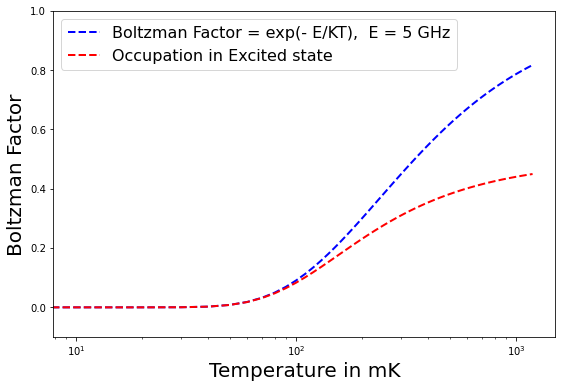
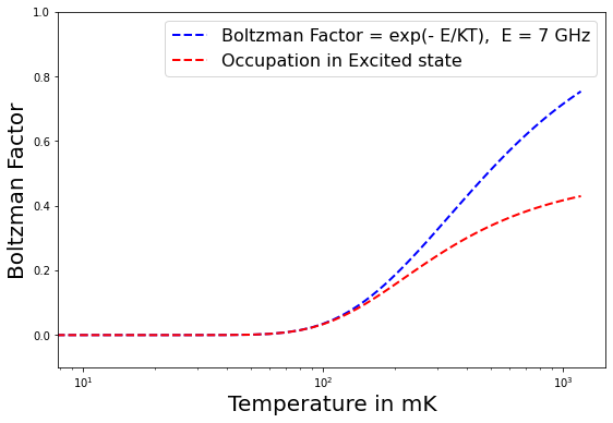
Figure 1: The Boltzmann factor and occupation probability of excited state as a function of temperature for two values of difference of energy levels between two states.

The main components of a quantum device are qubits coupled to a resonator which is driven by microwaves.

4 The resonator

The first step of design is a classical simulation of the resonator and transmon model. Many kinds of resonators can be considered Reagor_2016 . We consider a rectangular resonator with dimensions 36 mm $\times$ 6 mm $\times$ 22 mm. Aluminium EC grade (99.7%) with surface roughness, 0.5 microns is used in the simulation. The frequency is given by

$$f={\omega_{r}\over 2\pi}\,=\,{c\over 2}\,\sqrt{\left({n_{x}\over L_{x}}\right)^{2}+\left({n_{y}\over L_{y}}\right)^{2}+\left({n_{z}\over L_{z}}\right)^{2}}.$$ (15)

TE₁₁₀ mode is 8 GHz and the finite element (FE) simulation gives 7.75 GHz with a quality factor of 4268. For Al 6061 (97.9% purity) the quality factor is reduced. A transmon can be modeled as a lumped element with large capacitive pads on a silicon substrate. The junction is modeled as a rectangular sheet (200 $\mu$m $\times$ 50 $\mu$m) with a polyline with the current flow direction. An inductance is assigned to the junction.

We also use a $\lambda/4$ type of resonator. Height of stub is taken as 8 mm with inner radius 1 mm. Height of cylinder is taken as 30 mm with a radius 7 mm. One can obtain a rough estimate by $f={c/4L}$. The FE simulations give 7.6 GHz with $Q$ factor as 2909.

Dissipation ($\kappa$) in resonators is inversely related to Quality Factor $Q=\omega/\kappa$. Dissipation for a rectangular cavity depends on three factors;

• Dielectric loss which is due to oxide layer with thickness $t$.

• Conductor loss which depends on surface penetration depth ($\lambda$).

• Seam loss which is due to seam location. The seam loss is zero if the seam is exactly at the middle. It depends on machining tolerance $\delta x_{0}$.

Dissipation for $\lambda/4$ cavity depends on

• Conductor loss: $1/Q_{C}=\frac{2\sqrt{\pi\,f\mu\sigma}\,\ln(b/a)}{{1\over a}+{1\over b}}$,
  $a$ is the radius of the inner cylinder and $b$ is the radius of the outer cylinder, $\mu$ is the permeability and $\sigma$ is the conductivity of the conductor.

• Dielectric loss: $1/Q_{d}=1/\tan(\delta)$.

5 Quantum simulation

After the classical simulation of resonator and transmon, the electromagnetic circuit is then quantized and Hamiltonian parameters are obtained using Energy Partition Ratio method.

Hamiltonian for a single qubit-cavity system is given by Jaynes_1963 ; Shore_1993

$$H = H_{r}+H_{q}+H_{int}$$ (16)

$$= \omega_{r}\hat{a}^{\dagger}\hat{a}-\frac{1}{2}\omega_{q}\sigma_{z}+g\,(\hat{a}\sigma_{+}+\hat{a}^{\dagger}\sigma_{-}).$$

where $\omega_{q}$ is qubit frequency and $\omega_{r}$ is cavity frequency and $g$ is the coupling strength between them. This Hamiltonian can be solved in two modes. The polariton mode where $\triangle=\omega_{q}-\omega_{r}\simeq 0$ and dispersive mode, where $\chi=g^{2}/\triangle<<1$.

Hamiltonian for Qubit-Cavity system in dispersive limit is given by schuster2007 ; Boissonneault_2009

$$H = \omega_{r}\hat{a}^{\dagger}\hat{a}-\frac{1}{2}(\omega_{q}-\alpha/2)\sigma_{z}+\chi(\hat{a}^{\dagger}\hat{a}+1/2)\sigma_{z}.$$ (17)

Here $\alpha$ is self kerr and $\chi=g^{2}/\triangle$ is cross kerr.

The Hamiltonian for two coupled qubits is given by

$$H=-\frac{1}{2}\omega_{1}\sigma_{z1}-\frac{1}{2}\omega_{2}\sigma_{z2}+g\,\sigma_{y1}\sigma_{y2}.$$ (18)

Here $\omega_{1}$ and $\omega_{2}$ are the frequencies of the two transmons and $g$ is the coupling strength between them. The parameters of the Hamiltonian are obtained by pyEPR simulation Minev_2019 . The zero point fluctuations $\sqrt{\xi_{mJ}}$ are related to the $p_{mJ}$ which is the Energy Participation Ratio defined as Minev_2019

$$p_{mJ}=\frac{{\rm Inductive\,\,energy\,\,stored\,\,in\,\,junction\,\,}J}{{\rm Inductive\,\,energy\,\,stored\,\,in\,\,the\,\,mode\,\,}m}.$$ (19)

Figure 2 shows pyEPR simulations of a qubit coupled to a rectangular cavity giving modal frequencies (MHz), Anharmonicity $\alpha$ (MHz) and cross-kerr frequency $\chi$ (MHz) as a function of different values of $L$. For input parameter $L_{J}=6$ nH, $E_{J}=27.31$ GHz, the EPR value is 0.8 and $\omega_{r}/2\pi=$ 7.577 GHz, $\omega_{q}/2\pi=$ 6.794 GHz, $\alpha/2\pi=$ 190 MHz, $\chi/2\pi=$ 34.4 MHz which gives $g/2\pi=\sqrt{\chi\triangle}=$ 181 GHz.

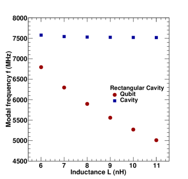
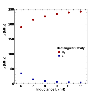
Figure 2: pyEPR simulations of a qubit coupled to a rectangular cavity showing modal frequencies (MHz), Anharmonicity $\alpha$ (MHz) and cross-kerr frequency $\chi$ (MHz) as a function of different values of $L$.

Figure 3 shows the pyEPR simulations of a qubit coupled to a rectangular cavity giving modal frequencies (MHz), Anharmonicity $\alpha$ (MHz) and cross-kerr frequency $\chi$ (MHz) as a function of different values of $L$. For input parameter $L_{J}=6$ nH, $E_{J}=27.31$ GHz, the EPR value is 0.76 and $\omega_{r}/2\pi=7.481$ GHz, $\omega_{q}/2\pi=6.229$ GHz, $\alpha/2\pi=162$ MHz, $\chi/2\pi=23.2$ MHz which gives $g/2\pi=\sqrt{\chi\triangle}=178$ MHz.

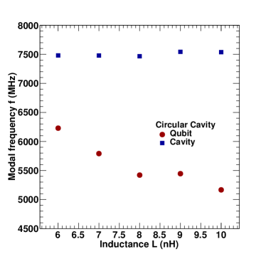
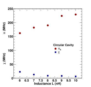
Figure 3: pyEPR simulations of a qubit coupled to a rectangular cavity showing modal frequencies (MHz), Anharmonicity $\alpha$ (MHz) and cross-kerr frequency $\chi$ (MHz) as a function of different values of $L$.

Figure 4 shows pyEPR simulations of 2 coupled qubits giving modal frequencies, anharmonicities ($\alpha_{0}$, $\alpha_{1}$) and cross-kerr frequency $\chi$. The variations correspond to the inductance of first junction as 6 nH and different values of inductance of the second junction. Table 2 shows the results of pyEPR simulation of two junctions with inductances 6 and 8 nH coupled to a rectangular cavity.

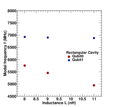
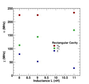
Figure 4: pyEPR simulations of 2 coupled qubits showing modal frequencies (MHz), anharmonicities (MHz) and cross-kerr frequencies (MHz). The variations correspond to the inductance of first junction as 6 nH and different values of inductance of the second junction.

Table 2: The results of pyEPR simulation for a rectangular cavity coupled to two Josephson junctions for input inductance 6 and 8 nH.

Mode	$\omega_{q}/2\pi$	$\alpha$	$\chi_{01}/2\pi$	$g/2\pi=\sqrt{\chi_{01}\triangle}$
0	6.926 GHz	225 MHz	79.8 MHz	306 MHz
1	5.755 GHz	113 MHz	79.8 MHz	306 MHz

6 Evolution of the open quantum system

In the previous section, we got a quantitative idea about the Hamiltonian parameters like frequencies, self-kerr, and cross-kerrs for our design. Once Hamiltonian parameters are obtained for the circuit, the energy levels of the system can be calculated. The dynamics of the system can be obtained using Lindblad master equation Manzano_2020 . This yields frequency spectrum, time spectrum, entanglement measures and calibration of microwave pulses. The time evolution of the density matrix is given by Lindblad equation as follows

$${\partial\over\partial t}\rho=-{i\over\hbar}[\hat{H}(t),\rho(t)]+\sum_{n}\frac{1}{2}\left[2L_{n}\rho(t)L_{n}^{+}-\rho(t)L_{n}^{+}L_{n}-L_{n}^{+}L_{n}\rho(t)\right].$$ (20)

Here, $\rho=\ket{\Psi}\bra{\Psi}$ is the density matrix and $L_{n}=\sqrt{\gamma_{n}}A_{n}$ are collapse or jump operators.

Von Neumann entropy which is an extension of Gibbs entropy $S=k\ln Z$ is given by

$$S=-\sum_{i}\|c_{i}\|^{2}\,\ln\|c_{i}\|^{2}=-Tr(\rho\ln\rho).$$ (21)

If $\ket{\Psi_{AB}}=\ket{\Psi_{A}}\ket{\Psi_{B}}$ is a separable state then entropy is zero. Then the reduced density matrix $\rho_{A}=Tr_{B}(\ket{\Psi_{AB}}\bra{\Psi_{AB}})=\ket{\Psi_{A}}\bra{\Psi_{A}}$ is a pure state. The entanglement is characterized by non-zero entropy.

The qubit can relax in two ways; longitudinal and transverse relaxation. The longitudinal relaxation is actually energy decay and can be expressed as jump operators for resonator gaining or losing a photon from a bath statistical2008

$$L_{\uparrow}=\sqrt{\kappa_{\uparrow}}\,\hat{a}^{\dagger},\,\,\,\,\,\,\,\,L_{\downarrow}=\sqrt{\kappa_{\downarrow}}\,\hat{a}.$$ (22)

The ratio of excitation and relaxation rates can be obtained in terms of Boltzmann factor

$$\frac{\kappa_{\uparrow}}{\kappa_{\downarrow}}=e^{-\hbar\omega/kT}.$$ (23)

Both the rates can be obtained in terms of single dissipation rate $\kappa_{1}$ and thermal occupancy $n_{th}$ as

$$\kappa_{\downarrow}=(1+n_{th})\kappa_{1},\,\,\,\,\,\kappa_{\uparrow}=n_{th}\kappa_{1},$$ (24)

where

$$n_{th}=\frac{1}{e^{\hbar\omega/kT}-1}.$$ (25)

Similarly, for the qubit

$$L_{q}=\sqrt{\Gamma_{1}}\,\sigma^{-}.$$ (26)

Decoherence or pure phase decay arises due to frequency change. The resonant frequency can be modified due to the scattering process of bath quantum and the jump operator can be modeled as statistical2008

$$L_{c\phi}=\sqrt{\kappa_{\phi}}\,\hat{a}^{\dagger}\hat{a}.$$ (27)

For the qubit,

$$L_{q\phi}=\sqrt{\Gamma_{\phi}}\,\sigma^{+}\sigma^{-}.$$ (28)

The transverse relaxation includes longitudinal relaxation and pure dephasing and are given for the resonator and the qubit as

$$\kappa_{2} = \kappa_{1}/2+\kappa_{\phi}\equiv\kappa,$$

$$\Gamma_{2} = \Gamma_{1}/2+\Gamma_{\phi}\equiv\Gamma.$$ (29)

The dissipation in the cavity varies as a function of temperature. Figure 5 shows the ratio of quality factor of aluminum cavity with the quality factor at 200 mK as a function of temperature Reagor_2013 .

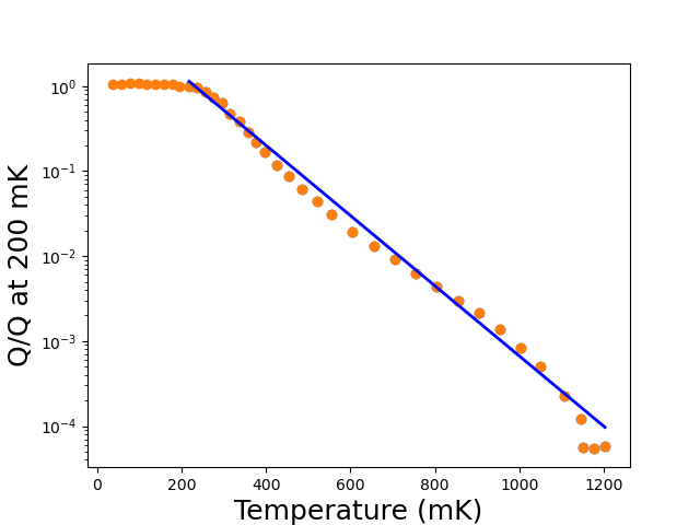
Figure 5: The ratio of quality factor of aluminium cavity with the quality factor at 200 mK as a function of temperature Reagor_2013 along with an exponential function.

The quality factor has been fitted by an exponential function

$$Q/Q_{200mK} = 9.06\,\exp(-T/105)\,\,\,(T\,{\rm in\,mK}).$$ (30)

From this, we can get the quality factor at 1 K as follows

$$Q_{1000mK} = 0.00015\times Q_{200mK}$$ (31)

$$= 0.00015\times(7\times 10^{7})=10500.$$

This corresponds to longitudinal dissipation in cavity as $\kappa_{1}/(2\pi)=\nu/Q=0.5$ MHz. Assuming pure dephasing rate as 0.25 MHz the transverse relaxation $\kappa_{2}/(2\pi)=\nu/(2Q)=0.25$ MHz + 0.25 MHz. The dissipations in superconducting qubits are of the order of $\Gamma/2\pi$ = $0.01$ MHz Reagor_2016 .

Figure 6 shows entropy for two qubits entanglement as a function of coupling strength for $\kappa/2\pi=10^{-5}$ MHz (cavity), $\Gamma/2\pi=10^{-5}$ MHz and Temperature at 200 mK. Table 2 shows that the coupling between the two qubits obtained is 306 MHz which corresponds to entropy 0.85 in Fig. 6 showing a high degree of entanglement.

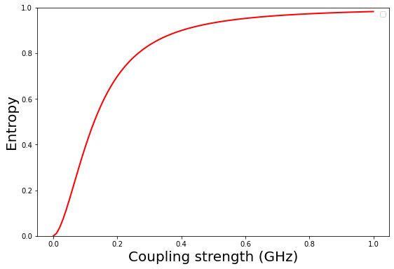
Figure 6: Entropy for two qubits entanglement as a function of coupling strength for $\kappa/2\pi=10^{-5}$ MHz (cavity), $\Gamma/2\pi=10^{-5}$ MHz and Temperature at 200 mK.

7 Rabi Oscillation

In this section, we present the results of the Rabi oscillation Wallraff2004 in a qubit-cavity system calculated using Lindablad equations with a set of realistic parameters. Rabi oscillations for a qubit-cavity system for parameters $\omega_{r}/2\pi$ = 7 GHz, $\omega_{q}/2\pi$ = 7 GHz, coupling $g$ = 200 MHz, $\kappa/2\pi$ = $10^{-5}$ MHz (cavity), $\Gamma/2\pi$ = $0.01$ MHz and $T$ = 200 mK are given in Fig. 7. Here we start with 5 photons in the cavity and one photon is exchanged between the qubit and cavity. It shows that the Rabi oscillations can be very well observed at 200 mK.

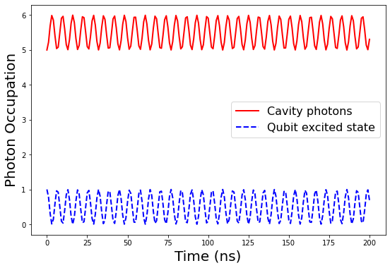
Figure 7: Rabi oscillations for a system for parameters $\omega_{r}/2\pi$ = 7 GHz, $\omega_{q}/2\pi$ = 7 GHz, coupling $g$ = 200 MHz, $\kappa/2\pi$ = $10^{-5}$ MHz (cavity), $\Gamma/2\pi$ = $0.01$ MHz and $T$ = 200 mK.

Rabi oscillations for a qubit-cavity system for parameters $\omega_{r}/2\pi$ = 7 GHz, $\omega_{q}/2\pi$ = 7 GHz, coupling $g$ = 200 MHz, $\kappa/2\pi$ = 0.5 MHz (cavity), $\Gamma/2\pi$ = $0.01$ MHz and $T$ = 200 mK are given in Fig. 8. Here we have increased the dissipation in the cavity corresponding to $\kappa/2\pi$ = 0.5 MHz which has made the oscillations die down within 100 ns.

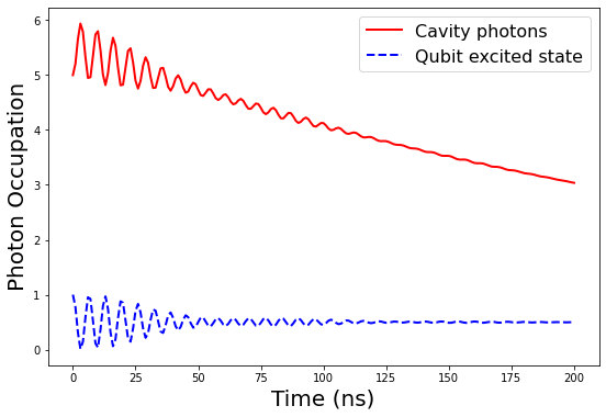
Figure 8: Rabi oscillations for a system for parameters $\omega_{r}/2\pi$ = 7 GHz, $\omega_{q}/2\pi$ = 7 GHz, coupling $g$ = 200 MHz, $\kappa/2\pi$ = 0.5 MHz (cavity) and $\Gamma/2\pi$ = $0.01$ MHz and $T$ = 200 mK.

Rabi oscillations for a system for parameters $\omega_{r}/2\pi$ = 7 GHz, $\omega_{q}/2\pi$ = 7 GHz, coupling $g$ = 200 MHz, $\kappa/2\pi$ = 0.5 MHz (cavity), $\Gamma/2\pi$ = $0.01$ MHz and $T$ = 1 K are given in Fig. 9. Here we have added dissipation in the cavity corresponding to $\kappa/2\pi$ = 0.5 MHz and also increased the temperature to 1 K which has made the oscillations die down within 30 ns.

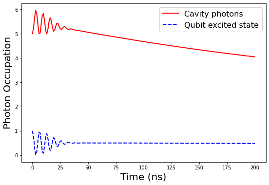
Figure 9: Rabi oscillations for a system for parameters $\omega_{r}/2\pi$ = 7 GHz, $\omega_{q}/2\pi$ = 7 GHz, coupling $g$ = 200 MHz, $\kappa/2\pi$ = 0.5 MHz (cavity), $\Gamma/2\pi$ = $0.01$ MHz and $T$ = 1 K.

8 Driven qubit

Hamiltonian for a qubit driven by a microwave signal is Naghiloo_2019

$$H=-{1\over 2}\omega_{q}\,\sigma_{z}+\Omega\,V_{d}(t)\sigma_{y}.$$ (32)

Applying $V_{d}(t)=V_{0}\cos(\omega_{d}t)$ and defining $g=\Omega V_{0}$ MHz we obtain

$$\hat{H}=-\frac{1}{2}w_{q}\sigma_{z}+g\,\cos(\omega_{d}t)\sigma_{y}.$$

The probability of qubit being in an excited state is obtained as

$$P_{e}(t)={g^{2}\over\Omega_{R}^{2}}\,\sin^{2}\left(\Omega_{R}t\over 2\right).$$

Here, $\Omega_{R}=\sqrt{g^{2}+(\omega_{q}-\omega_{d})^{2}}$. Figure 10 shows the Rabi oscillations driven by a microwave signal with coupling strength $g\sim 500$ MHz for $\omega_{q}=\omega_{d}$ .

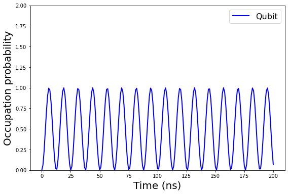
Figure 10: Rabi oscillations driven by a microwave signal with coupling strength $g\sim 500$ MHz for $\omega_{q}=\omega_{d}$.

Figure 11 shows a setup with a microwave (MW) drive mixed with an envelope function $S(t)$ generated using Arbitrary Wave Generator (AWG) and given to qubit. The resultant drive voltage is

$$V_{d}(t)=S(t)\,V_{0}\,\sin(\omega_{d}t+\phi).$$ (33)

Figure 12 shows a microwave pulse ($f=\omega_{d}/2\pi$=1 GHz for demonstration) with a sine envelope function with a frequency 10 MHz. The envelope function $S(t)=\sin(\omega_{e}t)$ with $\omega_{e}=10$ MHz is used in the calculations.

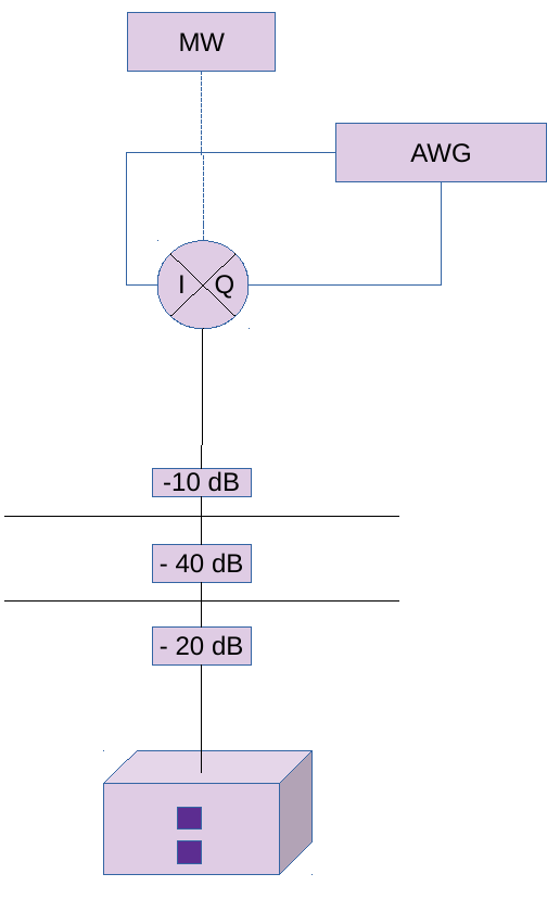
Figure 11: A setup with microwave drive mixed with an envelope function and given to qubit.

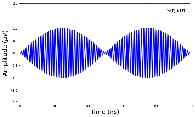
Figure 12: The microwave pulse with a sine envelope function with frequency 10 MHz.

The qubit can be manipulated using microwave pulses. The time duration of pulse for qubit rotation $\Theta$ can be obtained by solving

$$\Theta(t)=-g\int_{0}^{t}S(t^{\prime})dt^{\prime}.$$ (34)

Figure 13 shows the $\pi$ pulse (duration $t=17.6$ ns) which can be used for reversing the state of the qubit and $\pi/2$ pulse ($t=21.4$ ns) is used to put it in a superposition state.

Figure 13: The $\pi$ pulse (duration $t=17.6$ ns) which can be used for reversing the state of the qubit and $\pi/2$ pulse ($t=21.4$ ns) is used to put it in a superposition state.

9 Measurement of frequency shift

Figure 14 shows an experimental setup for frequency sweep. Here a signal from Vector Network Analyser (VNA) is sent to qubit and frequency sweep is done. The transmitted signal (S21) is measured via the 2nd port.

Figure 14: An experimental setup for frequency sweep.

Figure 15 shows the frequency shift of the cavity due to qubit for $\triangle=$ 1 GHz, $\chi/2\pi=$ 6 MHz and temperature = 200 mK. Left figure is for $\kappa/2\pi=$ 0.1 MHz and the right figure is for $\kappa/2\pi=$ 0.5 MHz. It is observed that the width of the lines is increased but they are well separated and will give the measure of qubit frequency.

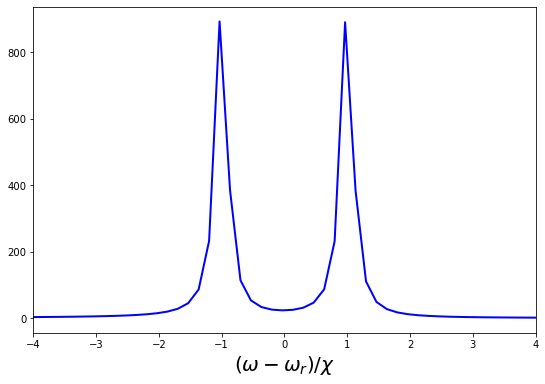
Figure 15: Frequency shift of the cavity due to qubit for $\triangle=$ 1 GHz, $\chi/2\pi=$ 6 MHz and temperature = 200 mK. Left figure is for $\kappa/2\pi=$ 0.1 MHz and the right figure is for $\kappa/2\pi=$ 0.5 MHz.

Figure 16 shows the frequency shift of the cavity due to qubit for $\triangle=$ 1 GHz, $\chi/2\pi=$ 6 MHz and temperature = 1000 mK. Left figure is for $\kappa/2\pi=$ 0.5 MHz and right figure is for $\kappa/2\pi=$ 1 MHz. It is observed that the width of the lines is increased but the difference can still be measured. For dissipation beyond $\kappa/2\pi>$ 1 MHz, the two lines merge. We can conclude that it is still possible to measure the frequency shift if the quality of the resonator is good.

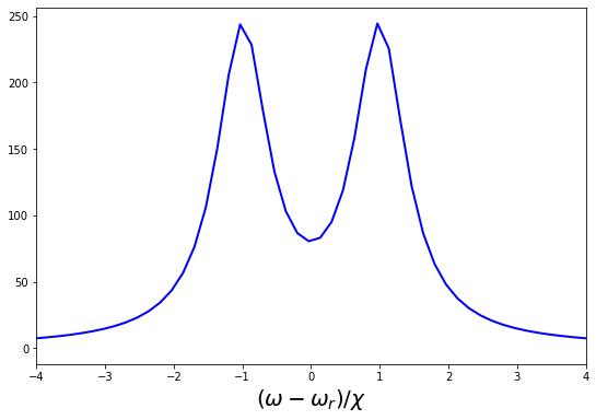
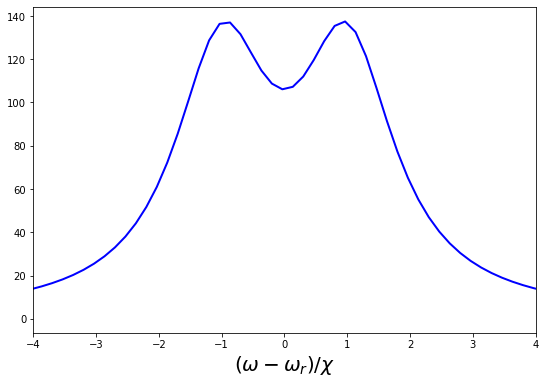
Figure 16: Frequency shift of the cavity due to qubit for $\triangle=$ 1 GHz, $\chi/2\pi=$ 6 MHz and temperature = 1000 mK. Left figure is for $\kappa/2\pi=$ 0.5 MHz and right figure is for $\kappa/2\pi=$ 1 MHz.

10 Summary

We presented a study of the dynamics of superconducting qubits coupled with cavity by including dissipation in sub kelvin temperature range. All the steps starting with a classical simulation, EPR method and Lindblad equation have been described. Once we have the parameters of Hamiltonian we can solve a quantum mechanical equation. An open quantum system formalism is implemented to study the effect of dissipation and finite temperature on the dynamics. Calculations are performed using a realistic set of dissipative parameters and include temperatures up to 1 K. Finally, we get frequency spectra and/or dynamics of the system with time with quantum effects. Such devices work at tens of milli Kelvins and quantum effects diminish as we move to higher temperatures. We find a set of parameters for which one can observe quantum behaviour up to 1 K for a resonator with a fairly good quality factor.

Data Availability Statement

The datasets generated during and/or analysed during the current study are available from the corresponding author on reasonable request.

References

- (1) J. P. Dowling, G. Milburn, Quantum technology: the second quantum revolution, Phil. Trans. R. Soc. A. 361 (2003) 1655.
- (2) M. A. Nielsen, I. L. Chuang, Quantum Computation and Quantum Information: 10th Anniversary Edition, Cambridge University Press, 2010.
- (3) T. Ladd, F. Jelezko, R. Laflamme, et al., Quantum computers, Nature 464 (2010) 45–53.
- (4) C. L. Degen, F. Reinhard, P. Cappellaro, Quantum sensing, Rev. Mod. Phys. 89 (2017) 035002.
- (5) Y. Nakamura, Y. A. Pashkin, J. S. Tsai, Coherent control of macroscopic quantum states in a single-cooper-pair box, Nature 398 (6730) (1999) 786–788.
- (6) J. Koch, T. M. Yu, J. Gambetta, A. A. Houck, D. I. Schuster, J. Majer, A. Blais, M. H. Devoret, S. M. Girvin, R. J. Schoelkopf, Charge-insensitive qubit design derived from the cooper pair box, Physical Review A 76 (4) (2007) 042319.
- (7) S. M. Girvin, M. H. Devoret, R. J. Schoelkopf, Circuit QED and engineering charge-based superconducting qubits, Physica Scripta T137 (2009) 014012.
- (8) A. Blais, J. Gambetta, A. Wallraff, D. I. Schuster, S. M. Girvin, M. H. Devoret, R. J. Schoelkopf, Quantum-information processing with circuit quantum electrodynamics, Physical Review A 75 (3) (2007) 032329.
- (9) J. M. Martinis, M. Devoret, J. Clarke, Quantum josephson junction circuits and the dawn of artificial atoms, Nat. Phys. 16 (2020) 234–237.
- (10) P. Krantz, M. Kjaergaard, F. Yan, T. P. Orlando, S. Gustavsson, W. D. Oliver, A quantum engineer's guide to superconducting qubits, Applied Physics Reviews 6 (2) (2019) 021318.
- (11) M. Naghiloo, Introduction to experimental quantum measurement with superconducting qubits, arXiv:1904.09291.
- (12) Z. K. Minev, S. O. Mundhada, S. Shankar, P. Reinhold, R. Gutiérrez-Jáuregui, R. J. Schoelkopf, M. Mirrahimi, H. J. Carmichael, M. H. Devoret, To catch and reverse a quantum jump mid-flight, Nature 570 (7760) (2019) 200–204.
- (13) D. Manzano, A short introduction to the lindblad master equation, AIP Advances 10 (2) (2020) 025106.
- (14) N. Didier, E. A. Sete, M. P. da Silva, C. Rigetti, Analytical modeling of parametrically modulated transmon qubits, Phys. Rev. A 97 (2) (2018) 022330.
- (15) V. Ambegaokar, A. Baratoff, Phys. Rev. Lett. 11 (1963) 104.
- (16) M. Reagor, W. Pfaff, C. Axline, R. W. Heeres, N. Ofek, K. Sliwa, E. Holland, C. Wang, J. Blumoff, K. Chou, M. J. Hatridge, L. Frunzio, M. H. Devoret, L. Jiang, R. J. Schoelkopf, Quantum memory with millisecond coherence in circuit QED, Physical Review B 94 (1) (2016) 014506.
- (17) E. Jaynes, F. Cummings, Comparison of quantum and semiclassical radiation theories with application to the beam maser, Proceedings of the IEEE 51 (1) (1963) 89–109.
- (18) B. Shore, P. Knight, The jaynes-cummings model, Journal of Modern Optics 40 (7) (1993) 1195–1238.
- (19) D. Schuster, A. Houck, J. Schreier, et al., Resolving photon number states in a superconducting circuit, Nature 445 (2007) 515–518.
- (20) M. Boissonneault, J. M. Gambetta, A. Blais, Dispersive regime of circuit QED: Photon-dependent qubit dephasing and relaxation rates, Physical Review A 79 (1) (2009) 013819.
- (21) H. J. Carmichael, Statistical Methods in Quantum Optics 2: Non-Classical Fields, Springer, 2008.
- (22) M. Reagor, H. Paik, G. Catelani, L. Sun, C. Axline, E. Holland, I. M. Pop, N. A. Masluk, T. Brecht, L. Frunzio, M. H. Devoret, L. Glazman, R. J. Schoelkopf, Reaching 10 ms single photon lifetimes for superconducting aluminum cavities, Applied Physics Letters 102 (19) (2013) 192604.
- (23) A. Wallraff, D. I. Schuster, A. Blais, L. Frunzio, R. S. Huang, J. Majer, S. Kumar, S. M. Girvin, R. J. Schoelkopf, Strong coupling of a single photon to a superconducting qubit using circuit quantum electrodynamics, Nature 431 (7005) (2004) 162–167. arXiv:cond-mat/0407325.