TNT: Vision Transformer for Turbulence Simulations

Abstract

Turbulence is notoriously difficult to model due to its multi-scale nature and sensitivity to small perturbations. Classical solvers of turbulence simulation generally operate on finer grids and are computationally inefficient. In this paper, we propose the Turbulence Neural Transformer (TNT), which is a learned simulator based on the transformer architecture, to predict turbulent dynamics on coarsened grids. TNT extends the positional embeddings of vanilla transformers to a spatiotemporal setting to learn the representation in the 3D time-series domain, and applies Temporal Mutual Self-Attention (TMSA), which captures adjacent dependencies, to extract deep and dynamic features. TNT is capable of generating comparatively long-range predictions stably and accurately, and we show that TNT outperforms the state-of-the-art U-net simulator on several metrics. We also test the model performance with different components removed and evaluate robustness to different initial conditions. Although more experiments are needed, we conclude that TNT has great potential to outperform existing solvers and generalize to additional simulation datasets.

1 Introduction

Many areas of the science and engineering rely heavily on turbulent dynamics. Turbulent flow simulations are widely employed in a variety of fields such as aerospace (Mishra et al., 2019), weather (Mirocha et al., 2014), combustion (Pitsch, 2006), and medicine (Ha et al., 2017). Due to the complexity of temporal and spatial scales and the chaotic nature of turbulence (Berera & Ho, 2018; Duraisamy et al., 2019), in which tiny perturbations in initial conditions can result in huge changes in outcomes, turbulence prediction is a difficult task despite its extensive uses.

In recent decades, numerical solvers for simulating large and complicated turbulent dynamics have been developed (Kim & Menon, 1999; Kang et al., 2011). However, these solvers rely heavily on massive computational resources and high spatial and temporal resolutions. More recently, solvers based on learned Machine Learning (ML) models have emerged, including Graph Neural Networks (GNN) (Sanchez-Gonzalez et al., 2020; Li et al., 2020b; Pfaff et al., 2020) and Convolutional Neural Networks (CNN) (Pathak et al., 2020; Stachenfeld et al., 2021; Li et al., 2020a; Wang et al., 2020). ML methods are feasible and promising ways to build more connections between existing simulation results with real-world data and to automatically identify dependencies which are not explained by current physics and mathematical equations (Beck & Kurz, 2021).

Our contribution is to introduce the Turbulence Neural Transformer (TNT) to learn turbulent dynamics on coarse grids based on the attention mechanism as introduced in the Transformer model (Vaswani et al., 2017). TNT uses the Temporal Mutual Self Attention (TMSA) block (Liang et al., 2022) to extract dependencies from an input window and generate rolling predictions with an encoder-decoder Transformer. It does not require any domain-specific expertise and is capable of producing more consistent and accurate predictions than the compared benchmark across relatively long and unevenly sampled temporal ranges.

2 Related work

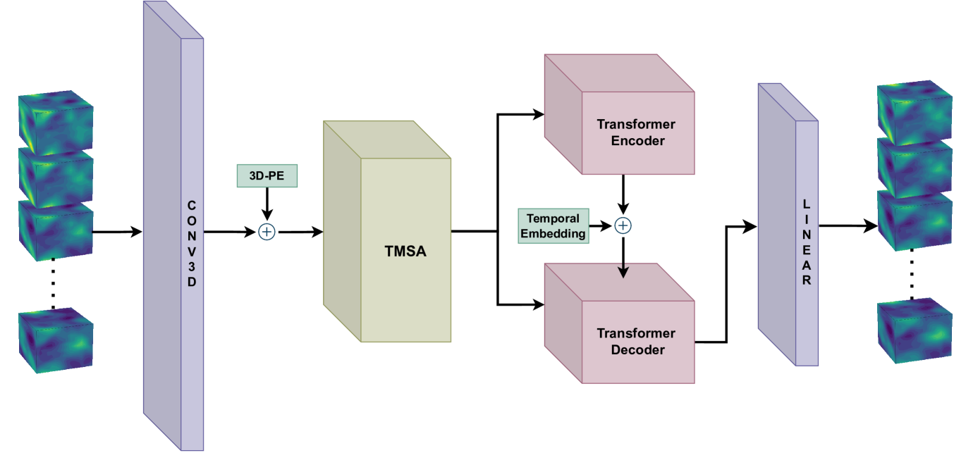
Figure 1: Framework of proposed Turbulence Neural Transformer (TNT) model. It takes a window of $16^{3}$ CompDecay-3D volumes as inputs and outputs a same-sized shifted window as predictions. TMSA and 3D-PE incorporate spatial information and temporal information is infused with temporal embedding.

Transformer networks (Vaswani et al., 2017) have been the state-of-the-art model for the majority NLP tasks since their introduction, along with other subsequent models based on the attention mechanism, such as BERT (Devlin et al., 2018) and RoBERTa (Liu et al., 2019). Recent studies have demonstrated the immense potential of using attention for multiple tasks in Computer Vision (CV) including object recognition in images (Dosovitskiy et al., 2020; Liu et al., 2021) and video restoration (Liang et al., 2022; Kim et al., 2018).

There are several previous studies on learned ML simulators for turbulence dynamics. Li et al. (2020a) built an efficient Fourier Neural Operator to solve PDEs including Navier-Stokes. Wang et al. (2020) employed learnt spectral filters and U-net to construct a Turbulence-Flow Net for turbulent predictions. Stachenfeld et al. (2021) implemented a general-purposed Dilated ResNet architecture to learn turbulent dynamics in a supervised setting without integrating specific domain knowledge. Our work is greatly inspired by studies of Dosovitskiy et al. (2020), Liang et al. (2022), and Stachenfeld et al. (2021). We take advantage of the recent advancements using Transformers in CV and apply those to modeling turbulence.

3 Data

Given a temporally unevenly sampled dataset $X\in\mathbb{R}^{N\times H\times W\times D\times C}$, where $N$ is the total number of 3-dimensional volumes ordered as a temporal sequence, $H,W,D$ are the grid size on the three spatial axes, and $C$ is the number of features. Denote $X_{i}$ as the $i$th volume, $\tau_{i}$ as the timestamp of $i$th volume, $\Delta\tau_{i}$ as the interval between the $\tau_{i}$ and $\tau_{i+1}$, and $x,y,z$ as the spatial coordinates each ranging from $0$ to the size of the corresponding spatial axes.

Data in this study are obtained from Athena++ (Stone et al., 2020), a state-of-the-art tool for astrophysical simulations. Specifically, we examine the 3D Compressible Decaying Turbulence (CompDecay-3D) with unevenly spaced temporal axis where $\tau$ ranges from $0$ to $1$. There are a total of 160 simulated volumes with grid size $16^{3}$. At each grid point, there are five features, namely gas density $\rho$, velocity vectors on the three spatial axes $v_{x},v_{y},v_{z}$, and gas pressure $P$. The goal is to predict the changes in densities $\Delta\rho_{i}$ between the current and the next volume given a current volume $X_{i}$ and a sequence of future timestamps $[\tau_{i+1},\tau_{i+2},\dots]$, with $\upsilon_{x},\upsilon_{y},\upsilon_{z},P$ as auxiliary features. There are two main challenges associated with CompDecay-3D. First, turbulence is a multi-scale physics phenomenon that necessitates extensive multi-scale computations. Given the coarse setting, it is particularly difficult because there is less available information from which the model may learn. Second, the time increment $\Delta t$ varies during the simulation, ranging from $4.3$ to $9.3$ milliseconds at roughly increasing temporal intervals throughout the simulation. Because of this inconsistency, the correlation between timestamps and turbulence dynamics needs to be adequately characterized.

4 Model

TNT is an attention-based model that learns the mapping $\boldsymbol{{\mathchoice{\raisebox{0.0pt}{$\displaystyle\chi$}}{\raisebox{0.0pt}{$\textstyle\chi$}}{\raisebox{0.0pt}{$\scriptstyle\chi$}}{\raisebox{0.0pt}{$\scriptscriptstyle\chi$}}}}\xrightarrow{}\boldsymbol{{\mathchoice{\raisebox{0.0pt}{$\displaystyle\chi$}}{\raisebox{0.0pt}{$\textstyle\chi$}}{\raisebox{0.0pt}{$\scriptstyle\chi$}}{\raisebox{0.0pt}{$\scriptscriptstyle\chi$}}}}$ where $\boldsymbol{{\mathchoice{\raisebox{0.0pt}{$\displaystyle\chi$}}{\raisebox{0.0pt}{$\textstyle\chi$}}{\raisebox{0.0pt}{$\scriptstyle\chi$}}{\raisebox{0.0pt}{$\scriptscriptstyle\chi$}}}}\subseteq\mathbb{R}^{5}$ and $X\in\boldsymbol{{\mathchoice{\raisebox{0.0pt}{$\displaystyle\chi$}}{\raisebox{0.0pt}{$\textstyle\chi$}}{\raisebox{0.0pt}{$\scriptstyle\chi$}}{\raisebox{0.0pt}{$\scriptscriptstyle\chi$}}}}$. Specifically, it takes a temporal window of volumes $[X_{i},X_{i+1},\dots,X_{i+w}]$ as inputs and output a shifted window of volumes $[\tilde{X}_{i+1},\tilde{X}_{i+2},\dots,\tilde{X}_{i+w+1}]$ as predictions, where $w$ is the window size. Figure 1 illustrates the architecture of TNT.

4.1 3D Positional Encoding

With a simple modification to the position encoding technique proposed in the transformer paper (Vaswani et al., 2017), we develop a 3D positional embedding (3D-PE). Three sets of 1D positional encodings are made separately on three spatial axes, each having one-third of the latent dimension size $d$. The final 3D-PE is constructed by concatenating three 1D encodings. Each grid point within the same volume receiving a unique encoding, whereas grid points with identical spatial coordinates at different timestamps receive identical encodings.

4.2 Temporal Embedding

Due to the unevenness on the temporal axis, instead of using fixed representations such as from a Fourier transformation of time values, we adopt a temporal embedding method named Time2Vec (Kazemi et al., 2019) that uses learned representations as the embedding values. For a given scalar of time $\tau$ , Time2Vec of $\tau$, denoted as $\vec{t2v}(\tau)$, is a vector of size k + 1 defined as follows:

$$\vec{t2v}(\tau)[i]=\begin{cases}\omega_{i}\tau+\varphi_{i}&\textbf{if $i=0$}\\ \digamma(\omega_{i}\tau+\varphi_{i})&\textbf{if $1\leq i\leq k$}\end{cases}$$ (1)

where $\vec{t2v}(\tau)[i]$is the ith element of $\vec{t2v}(\tau)$, $\digamma$ is a sine activation function, and $\omega$ is and $\varphi$ is are learnable parameters indicating correspondingly frequency and phase-shift.

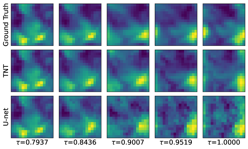
Figure 2: Visualization on predictions of U-net and TNT vs ground truth at five different timestamps from the beginning, $\tau=0.7937$, to the end, $\tau=1.0$, of the testing set. Each slice is taken at the middle of the volume across the third spatial axis $z$.

4.3 TMSA

Temporal Mutual Self-Attention is a feature alignment technique originally proposed, in Video Restoration Transformer (VRT)(Liang et al., 2022) paper, to extract interactions between adjacent frames in a video.

We modified the TMSA to make it compatible with 3D input and the periodic boundary condition when input windows are shifted. Each layer in the 3D-TMSA block takes a window of volumes and partitions it into non-overlapping two-volumes windows which are further partitioned into pairs of smaller patches. Following the same idea as in VRT, we apply 3D-TMSA on each pair of patches and shift the entire window of volumes on the three spatial axes and the temporal axis. As a result, the output of the 3D-TMSA block provides information on both temporal and spatial interaction within an input window of volumes.

4.4 Transformer

We follow the same architecture of the vanilla Transformer (Vaswani et al., 2017) with minor modifications. Transformer’s input volumes are partitioned into patches in the same manner as TMSA. Input to the decoder is a right-shifted window of the encoder’s input along the temporal axis with the last volume filled with zeros. The Transformer’s output is then fed into a simple linear layer that generates predictions.

4.5 Boundary condition

Due to the periodic boundary condition in the dataset, all the methods used in this study have been specifically configured or modified to capture the correlations across the boundaries.

5 Experiments

5.1 Benchmark

We compare TNT’s performance with a 3D version of U-net (Ronneberger et al., 2015) where code is modified from ELEKTRONN team’s GitHub (Kornfeld et al., 2018). U-net has been a popular benchmark and shown competitive performance in numerous previous works (Stachenfeld et al., 2021; Li et al., 2020a; Pathak et al., 2020). Our implementation of U-net closely follows that in Stachenfeld et al. (2021) on choices of parameters and addition of training noise.

5.2 Evaluation Metrics

In this specific task, the criterion of the model performance is its ability to stably predict the turbulence density over time. Therefore, we selected Root Mean Squared Error (RMSE), Mean Absolute Error (MAE), R-Squared ($\text{R}^{2}$), and Explained Variance (EV) as our evaluation metrics. Detailed description and mathematical defination are in Appendix C. A better performance is indicated by smaller RMSE & MAE and larger $\text{R}^{2}$ & EV.

5.3 Training and fine-tuning

We split the CompDecay-3D dataset into training (60%), validation (20%), and testing (20%) sets chronologically on the temporal axis. Predictions are made in a rolling manner where previous predictions are used in generating subsequent ones and each rollout step consist of prediction on the entire $16^{3}$ volume. For parameter optimization, we employ a mean average error loss and an early stopping to prevent overfitting. We use 4 RTX8000 GPUs for all fine-tuning. The best set of hyperparameters is selected based on performance on the validation split. During inference, training is conducted on the combined training and validation sets using the chosen hyperparameters to generate predictions on the testing set.

6 Results

We plot the progression of different metrics vs. number of rollout steps for both U-net and our proposed model TNT in Figure 3. As a result of rolling prediction, errors from previous predictions are carried over to subsequent ones. As observed in the plots, both models show the accumulation of errors with longer rollout steps. Throughout the inference phases, TNT outperforms U-net with smaller initial errors and slower degradation in performance. As illustrated in Figure 2, TNT generates stable and accurate predictions after 30 rollout steps, whereas U-net’s predictions are noisy and less accurate. It is also observed in Table 1 that TNT performs better in all metrics with improvements of 35% in RMSE, 35% in MSE, 48% in $\text{R}^{2}$, and 52% in EV. TNT can effectively capture the multi-scaled dependencies in CompDecay-3D whereas U-net fails to generate predictions with longer rollout steps. Ablation studies and results on all features can be found in the Appendix A and B.

Table 1: Performance of TNT and U-net on the testing data

Model	RMSE	MAE	$\text{R}^{2}$	EV
TNT	0.0782	0.0561	0.8080	0.8239
U-net	0.1208	0.0864	0.5401	0.5410

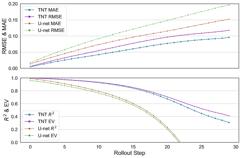
Figure 3: Comparison of performance between our proposed model TNT and U-net vs. number of rollout steps. TNT shows higher performance in all four evaluated metrics.

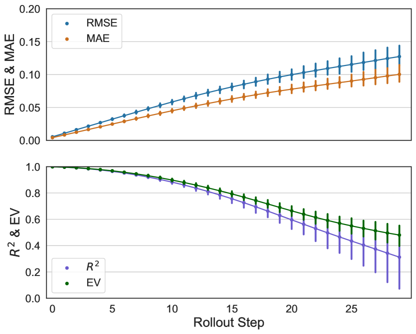
Figure 4: Generalization on 10 additional initial conditions. TNT is simply re-trained without further fine-tuning. No significant difference in performance from the primary result is observed acorss different initial conditions.

6.1 Generalization on different initial conditions

We also conduct experiments with ten distinct initial conditions, as slight variations in initial conditions can result in drastically different outcomes. Without further fine-tuning, we simply re-train the model with the same set of hyperparameters using the combined training and validation sets described in Section 5.3. Figure 4 shows the line plot with error bars for all ten trails. There is no large deviance from the performance observed in Figure 3. Since the exact same tuned parameters are used throughout all experiments, there is sufficient evidence to support our claim that TNT, with simple re-training, can generalize to all potential simulations in CompDecay-3D.

7 Conclusions

Turbulence prediction is a difficult task due to the complexities of temporal and spatial scales. We conduct experiments on predicting features in CompDecay-3D with 11 different initial conditions on coarse grids of $16^{3}$. Our proposed model, TNT, shows significantly lower RMSE and MAE and higher $\text{R}^{2}$ and EV than a U-net. Although TNT is robust to initial conditions in CompDecay-3D, additional experiments are needed to demonstrate its ability on generalizing to larger grid resolutions and longer rollout steps. We further show the importance of major components in our architecture in ablation studies in Appendix A, where significant drops in performance are observed with each component removed. The experimental results suggest that using attention to describe chaotic and complex simulations is feasible and effective. The two attention-based layers, TMSA and Transformer, can aid in the capture of spatial dependencies, while temporal embedding aids in the capture of temporal dependencies in rollout. Our proposed model shows great potential in generalizing well to a larger variety of simulations for which additional experiments are required.

Appendix A Ablation Studies

We inspect the performances of the model when a certain component is removed. Specifically, one of Transformer’s encoder, TMSA, and temporal embedding is deactivated while other parts of the architecture remain unchanged. We perform separate fine-tuning procedures, as described in Section 5.3, for each of the ’new’ architecture. Table A1 summarizes performances of this ablation study. We observe significant decrease in all four metrics when any of the three components is removed. Without temporal embedding, the model may lose important information on the temporal scale and unable to generate accurate predictions in longer rollout steps. This is further confirmed by the trend shown in Figure A.1 with progressive increases in RMSE and decreaess in $\text{R}^{2}$ throughout the inference. In the absence of TMSA, dependencies between volumes at different temporal and spatial scales may be largely lost, resulting in a immediate performance reduction, as seen in Figure A.1. The removal of the Transformer encoder appears to fall between the prior two cases where portions of spatial and temporal information are lost. We conclude that every layer in our proposed architecture is necessary and functions as expected in capturing the dependencies in and between temporal and spatial scales.

Table A1: Ablation studies on Transformer Encoder, TMSA, and temporal embedding

Model	RMSE	MAE	$\text{R}^{2}$	EV
TNT	0.0782	0.0561	0.8080	0.8239
$\times$ Encoder	0.1396	0.0998	0.3894	0.4066
$\times$ Tmsa	0.1371	0.1006	0.4073	0.4115
$\times$ Temporal Embedding	0.1572	0.1195	0.2253	0.6056

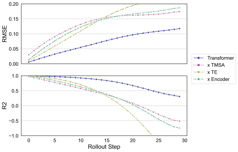
Figure A.1: Ablation studies on Transformer Encoder, TMSA, and temporal embedding. RMSE and $\text{R}^{2}$ drop when any component is removed from the architecture.

Appendix B Predictions on all features

We further provide visual results in Figure B.1. It shows slice plots on predictions of all five features at the end (step 30) of the rollout. It is clear that TNT stays robust even at long-range rolling prediction.

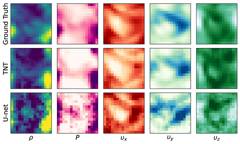
Figure B.1: Visualization of predictions on all features at 30th rollout step of TNT and U-net vs ground truth. Each slice is taken at the middle of the volume across the third spatial axis $z$.

Appendix C Definition of Evaluation Metrics

Denote $y$ to be the target variable we want to predict with size $n$, and $\hat{y}$ to be the model predictions. Suppose $\hat{y_{i}}$ is the $i$-th prediction with $y_{i}$ the corresponding ground truth, then the evaluation metrics Root Mean Squared Error (RMSE), Mean Absolute Error (MAE), R-Squared ($\text{R}^{2}$), and Explained Variance (EV) are defined as follows:

• $\text{RMSE}(y,\hat{y})=\sqrt{\frac{1}{n}\sum_{i=0}^{n-1}(y_{i}-\hat{y}_{i})^{2}}$

• $\text{MAE}(y,\hat{y})=\frac{1}{n}\sum_{i=0}^{n-1}\left|y_{i}-\hat{y}_{i}\right|$

• $\text{R}^{2}(y,\hat{y})=1-\frac{\sum_{i=1}^{n}(y_{i}-\hat{y}_{i})^{2}}{\sum_{i=1}^{n}(y_{i}-\bar{y})^{2}}$, where $\bar{y}=\frac{1}{n}\sum_{i=1}^{n}y_{i}$

• $\text{EV}(y,\hat{y})=1-\frac{Var\{y-\hat{y}\}}{Var\{y\}}$

RMSE calculates the expected value of the root of the squared loss or $l2$-norm loss, while MAE calculates the expected value of the absolute error loss or $l1$-norm loss. $\text{R}^{2}$ and EV represents the proportion of variance that has been explained by the model, and provides an indication of how well unseen samples are likely to be predicted by the model.

References

- Beck & Kurz (2021) Beck, A. and Kurz, M. A perspective on machine learning methods in turbulence modeling. GAMM-Mitteilungen, 44(1):e202100002, 2021.
- Berera & Ho (2018) Berera, A. and Ho, R. D. Chaotic properties of a turbulent isotropic fluid. Physical review letters, 120(2):024101, 2018.
- Devlin et al. (2018) Devlin, J., Chang, M.-W., Lee, K., and Toutanova, K. Bert: Pre-training of deep bidirectional transformers for language understanding. arXiv preprint arXiv:1810.04805, 2018.
- Dosovitskiy et al. (2020) Dosovitskiy, A., Beyer, L., Kolesnikov, A., Weissenborn, D., Zhai, X., Unterthiner, T., Dehghani, M., Minderer, M., Heigold, G., Gelly, S., et al. An image is worth 16x16 words: Transformers for image recognition at scale. arXiv preprint arXiv:2010.11929, 2020.
- Duraisamy et al. (2019) Duraisamy, K., Iaccarino, G., and Xiao, H. Turbulence modeling in the age of data. Annual Review of Fluid Mechanics, 51:357–377, 2019.
- Ha et al. (2017) Ha, H., Lantz, J., Ziegler, M., Casas, B., Karlsson, M., Dyverfeldt, P., and Ebbers, T. Estimating the irreversible pressure drop across a stenosis by quantifying turbulence production using 4d flow mri. Scientific reports, 7(1):1–14, 2017.
- Kang et al. (2011) Kang, S., Lightbody, A., Hill, C., and Sotiropoulos, F. High-resolution numerical simulation of turbulence in natural waterways. Advances in Water Resources, 34(1):98–113, 2011.
- Kazemi et al. (2019) Kazemi, S. M., Goel, R., Eghbali, S., Ramanan, J., Sahota, J., Thakur, S., Wu, S., Smyth, C., Poupart, P., and Brubaker, M. Time2vec: Learning a vector representation of time. arXiv preprint arXiv:1907.05321, 2019.
- Kim et al. (2018) Kim, T. H., Sajjadi, M. S. M., Hirsch, M., and Scholkopf, B. Spatio-temporal transformer network for video restoration. In Proceedings of the European Conference on Computer Vision (ECCV), September 2018.
- Kim & Menon (1999) Kim, W.-W. and Menon, S. An unsteady incompressible navier–stokes solver for large eddy simulation of turbulent flows. International Journal for Numerical Methods in Fluids, 31(6):983–1017, 1999.
- Kornfeld et al. (2018) Kornfeld, J., Drawitsch, M., Nguyen, M.-T., Pfeiler, N., Schubert, P., Dorkenwald, S., and Killinger, M. elektronn3. https://github.com/ELEKTRONN/elektronn3, 2018.
- Li et al. (2020a) Li, Z., Kovachki, N., Azizzadenesheli, K., Liu, B., Bhattacharya, K., Stuart, A., and Anandkumar, A. Fourier neural operator for parametric partial differential equations. arXiv preprint arXiv:2010.08895, 2020a.
- Li et al. (2020b) Li, Z., Kovachki, N., Azizzadenesheli, K., Liu, B., Bhattacharya, K., Stuart, A., and Anandkumar, A. Neural operator: Graph kernel network for partial differential equations. arXiv preprint arXiv:2003.03485, 2020b.
- Liang et al. (2022) Liang, J., Cao, J., Fan, Y., Zhang, K., Ranjan, R., Li, Y., Timofte, R., and Van Gool, L. Vrt: A video restoration transformer. arXiv preprint arXiv:2201.12288, 2022.
- Liu et al. (2019) Liu, Y., Ott, M., Goyal, N., Du, J., Joshi, M., Chen, D., Levy, O., Lewis, M., Zettlemoyer, L., and Stoyanov, V. Roberta: A robustly optimized bert pretraining approach. arXiv preprint arXiv:1907.11692, 2019.
- Liu et al. (2021) Liu, Z., Lin, Y., Cao, Y., Hu, H., Wei, Y., Zhang, Z., Lin, S., and Guo, B. Swin transformer: Hierarchical vision transformer using shifted windows. In Proceedings of the IEEE/CVF International Conference on Computer Vision, pp. 10012–10022, 2021.
- Mirocha et al. (2014) Mirocha, J., Kosović, B., and Kirkil, G. Resolved turbulence characteristics in large-eddy simulations nested within mesoscale simulations using the weather research and forecasting model. Monthly Weather Review, 142(2):806–831, 2014.
- Mishra et al. (2019) Mishra, A. A., Mukhopadhaya, J., Iaccarino, G., and Alonso, J. Uncertainty estimation module for turbulence model predictions in su2. AIAA Journal, 57(3):1066–1077, 2019.
- Pathak et al. (2020) Pathak, J., Mustafa, M., Kashinath, K., Motheau, E., Kurth, T., and Day, M. Using machine learning to augment coarse-grid computational fluid dynamics simulations. arXiv preprint arXiv:2010.00072, 2020.
- Pfaff et al. (2020) Pfaff, T., Fortunato, M., Sanchez-Gonzalez, A., and Battaglia, P. W. Learning mesh-based simulation with graph networks. arXiv preprint arXiv:2010.03409, 2020.
- Pitsch (2006) Pitsch, H. Large-eddy simulation of turbulent combustion. Annu. Rev. Fluid Mech., 38:453–482, 2006.
- Ronneberger et al. (2015) Ronneberger, O., Fischer, P., and Brox, T. U-net: Convolutional networks for biomedical image segmentation. In International Conference on Medical image computing and computer-assisted intervention, pp. 234–241. Springer, 2015.
- Sanchez-Gonzalez et al. (2020) Sanchez-Gonzalez, A., Godwin, J., Pfaff, T., Ying, R., Leskovec, J., and Battaglia, P. Learning to simulate complex physics with graph networks. In International Conference on Machine Learning, pp. 8459–8468. PMLR, 2020.
- Stachenfeld et al. (2021) Stachenfeld, K., Fielding, D. B., Kochkov, D., Cranmer, M., Pfaff, T., Godwin, J., Cui, C., Ho, S., Battaglia, P., and Sanchez-Gonzalez, A. Learned coarse models for efficient turbulence simulation. arXiv preprint arXiv:2112.15275, 2021.
- Stone et al. (2020) Stone, J. M., Tomida, K., White, C. J., and Felker, K. G. The athena++ adaptive mesh refinement framework: Design and magnetohydrodynamic solvers. The Astrophysical Journal Supplement Series, 249(1):4, June 2020. doi: 10.3847/1538-4365/ab929b. URL https://doi.org/10.3847%2F1538-4365%2Fab929b.
- Vaswani et al. (2017) Vaswani, A., Shazeer, N., Parmar, N., Uszkoreit, J., Jones, L., Gomez, A. N., Kaiser, Ł., and Polosukhin, I. Attention is all you need. In Advances in neural information processing systems, pp. 5998–6008, 2017.
- Wang et al. (2020) Wang, R., Kashinath, K., Mustafa, M., Albert, A., and Yu, R. Towards physics-informed deep learning for turbulent flow prediction. In Proceedings of the 26th ACM SIGKDD International Conference on Knowledge Discovery & Data Mining, pp. 1457–1466, 2020.