Predicting Opinion Dynamics via Sociologically-Informed Neural Networks

Abstract.

Opinion formation and propagation are crucial phenomena in social networks and have been extensively studied across several disciplines. Traditionally, theoretical models of opinion dynamics have been proposed to describe the interactions between individuals (i.e., social interaction) and their impact on the evolution of collective opinions. Although these models can incorporate sociological and psychological knowledge on the mechanisms of social interaction, they demand extensive calibration with real data to make reliable predictions, requiring much time and effort. Recently, the widespread use of social media platforms provides new paradigms to learn deep learning models from a large volume of social media data. However, these methods ignore any scientific knowledge about the mechanism of social interaction. In this work, we present the first hybrid method called Sociologically-Informed Neural Network (SINN), which integrates theoretical models and social media data by transporting the concepts of physics-informed neural networks (PINNs) from natural science (i.e., physics) into social science (i.e., sociology and social psychology). In particular, we recast theoretical models as ordinary differential equations (ODEs). Then we train a neural network that simultaneously approximates the data and conforms to the ODEs that represent the social scientific knowledge. In addition, we extend PINNs by integrating matrix factorization and a language model to incorporate rich side information (e.g., user profiles) and structural knowledge (e.g., cluster structure of the social interaction network). Moreover, we develop an end-to-end training procedure for SINN, which involves Gumbel-Softmax approximation to include stochastic mechanisms of social interaction. Extensive experiments on real-world and synthetic datasets show SINN outperforms six baseline methods in predicting opinion dynamics.

1. Introduction

Opinion dynamics is the study of information and evolution of opinions in human society. In society, people exchange opinions on various subjects including political issues, new products, and social events (e.g., sports events). As a result of such interactions (i.e., social interaction), an individual’s opinion is likely to change over time. Understanding the mechanisms of social interaction and predicting the evolution of opinions are essential in a broad range of applications such as business marketing (Sánchez-Núñez et al., 2020; Kumar et al., 2018), public voice control (Lai et al., 2018), friend recommendation on social networking sites (Eirinaki et al., 2013) and social studies (Moussaïd et al., 2013). For example, predicting the evolution of opinion dynamics can help companies design optimal marketing strategies that can guide the market to react more positively to their products.

Theoretical models called opinion dynamics models have been proposed for modeling opinion dynamics. The earliest work can be traced back to sociological and social psychological research by French (French Jr, 1956) and DeGroot (DeGroot, 1974). The most representative ones are bounded confidence models (Hegselmann and Krause, 2002; Deffuant et al., 2000), which take into account the psychological phenomenon known as confirmation bias — the tendency of people to accept only information that confirms prior beliefs. These models specify the underlying mechanism of social interaction in the form of difference equations. Typically, opinion dynamics models are explored and validated by computer simulations such as agent-based models. The theoretical models are highly interpretable; and can utilize the wealth of knowledge from social sciences, especially in social psychology and sociology. However, to learn predictive models, the computer simulations require calibration with real data, which incurs high manual effort and high computational complexity due to the massive data needed.

Nowadays, social media is increasingly popular as means of expressing opinions (O’Connor et al., 2010; Devi and Kamalakkannan, 2020) and they have become a valuable source of information for analyzing the formation of opinions in social networks. Data-driven methods have been applied to exploit large-scale data from social media for predicting the evolution of users’ opinions. For instance, De et al. (De et al., 2014) developed a simple linear model for modeling the temporal evolution of opinion dynamics. Some studies (De et al., 2016; Kulkarni et al., 2017) proposed probabilistic generative models based on point processes that capture the non-linear dynamics of opinion formation. However, these models lack flexibility as they use hand-crafted functions to model social interaction. Recent work (Zhu et al., 2020) developed a deep learning approach that automatically learns the social interaction and underlying evolution of individuals’ opinions from social media posts. While this approach enables flexible modeling of social interaction, it is largely agnostic to prior scientific knowledge of the social interaction mechanism.

In this paper, we propose a radically different approach that integrates both large-scale data and prior scientific knowledge. Inspired by the recent success of physics-informed neural networks (PINNs) (Raissi et al., 2019a), we extend them to encompass opinion dynamics modeling. To this end, we first reformulate opinion dynamics models into ordinary differential equations (ODEs). We then approximate the evolution of individuals’ opinions by a neural network. During the training process, by penalizing the loss function with the residual of ODEs that represent the theoretical models of opinion dynamics, the neural network approximation is made to consider sociological and social psychological knowledge.

While PINNs have successfully incorporated the laws of physics into deep learning, some challenges arise when translating this method to opinion dynamics. First, most of them fail to capture the stochastic nature of social interaction. Many recent opinion dynamics models involve stochastic processes that emulate real-world interactions. For example, several bounded confidence models encode probabilistic relationships between individuals, in which individuals randomly communicate their opinion to others, via stochastic variables. Such stochastic processes require sampling from discrete distributions, which makes backpropagating the error through the neural network impossible. Second, they cannot utilize additional side information including individuals’ profiles, social connections (e.g., follow/following relationship in Twitter), and external influences from mass media, government policy, etc. In real cases, we can obtain rich side information from social media, including user profiles and social media posts (e.g., user profile description and tweet text attributes), which is described in natural language. Finally, they cannot consider structural knowledge on social interaction. Social interaction is represented by network structure, and each network has a certain cluster structure. Previous studies have empirically shown real-world social networks consist of different user communities sharing same beliefs (Kumar et al., 2006).

To address these challenges, we develop a new framework called SINN (Sociologically-Informed Neural Network), which is built upon PINNs. To take account of the stochastic nature of opinion dynamics models, we incorporate the idea of reparameterization into the framework of PINNs. Specifically, we replace the discrete sampling process with a differentiable function of parameters and a stochastic variable with fixed Gumbel-Softmax distribution. This makes the gradients of the loss propagate backward through the sampling operation and thus the whole framework can be trained end-to-end. Also, PINNs are broadened to include rich side information. To use users’ profile descriptions, we combine the framework of PINNs and natural language processing techniques by adding a pre-trained language model. Moreover, building upon structural knowledge on the social interaction network (i.e., cluster structure), we apply low-rank matrix factorization to the parameters of ODEs. The proposal, SINN, incorporates the underlying sociology and social psychology, as described by ODEs, into the neural network as well as rich side information and structural knowledge, while at the same time exploiting the large amount of data available from social media.

To evaluate our proposed framework we conduct extensive experiments on three synthetic datasets and three real-world datasets from social networks (i.e., Twitter and Reddit). They demonstrate that SINN provides better performance for opinion prediction than several existing methods, including classical theoretical models as well as deep learning-based models. To the best of our knowledge, this work is the first attempt to transpose the concepts of PINNs from natural science (i.e., physics) into social science (i.e., sociology and social psychology). To foster future work in this area, we will release our code and sample data on https://github.com/mayaokawa/opinion_dynamics.

Our contributions are summarized as follows:

• We propose the first hybrid framework called SINN (Sociologically-Informed Neural Network) that integrates a large amount of data from social media and underlying social science to predict opinion dynamics in a social network.

• SINN formulates theoretical models of opinion dynamics as ordinary differential equations (ODEs), and then incorporates them as constraints on the neural network. It also includes matrix factorization and a language model to incorporate rich side information and structural knowledge on social interaction.

• We propose an end-to-end training procedure for the proposed framework. To include stochastic opinion dynamics models in our framework, we introduce the reparameterization trick into SINN, which makes its sampling process differentiable.

• We conduct extensive experiments on three synthetic datasets and three real-world datasets from social networks. The results show that SINN outperforms six existing methods in predicting the dynamics of individuals’ opinions in social networks.

2. Related Work

Physics-informed neural networks. From a methodological perspective, this paper is related to the emerging paradigm of physics-informed neural networks (PINNs) (Raissi et al., 2019a). PINNs incorporate physical knowledge into deep learning by enforcing physical constraints on the loss function, which is usually described by systems of partial differential equations (PDEs). These methods have been successfully applied to many physical systems, including fluid mechanics (Sun et al., 2020), chemical kinetic (Ranade et al., 2019), optics (Chen et al., 2020). This paper is the first attempt to import this approach into the field of social science, especially for modeling opinion dynamics. This poses three major challenges. First, many common opinion dynamics models involve randomized processes; but most PINNs deal only with deterministic systems. Very few works (Yang et al., 2020; Zhang et al., 2019) explore stochastic PDEs with additive noise terms. However, they still fail to model stochastic terms that contain the model parameters. Second, they do not include rich side information such as profiles of social media users and social media posts. Third, they cannot take into account extra structural knowledge on social interaction.

Opinion dynamics modeling. Opinion dynamics is the study of how opinions emerge and evolve through the exchange of opinions with others (i.e., social interaction). It has been a flourishing topic in various disciplines from social psychology and sociology to statistical physics and computer science. Theoretical models of opinion dynamics have been developed in divergent model settings with different opinion expression formats and interaction mechanisms. The first mathematical models can be traced back to works by sociologists and psychologists. In the 60s, French and John (French Jr, 1956) proposed the first simple averaging model of opinion dynamics, followed by Harary (Acemoğlu et al., 2013) and DeGroot (DeGroot, 1974). Extensions to this line of work, such as Friedkin and Johnsen (FJ) model (Friedkin and Johnsen, 1990), incorporated the tendency of people to cling to their initial opinions. Bounded confidence models, including Hegselmann-Krause (HK) model (Hegselmann and Krause, 2002) and Deffuant-Weisbuch (DW) model (Deffuant et al., 2000), consider confirmation bias: the tendency of individuals to interact those with similar opinions. Later studies generalized bounded confidence models to account for multi-dimensional opinion spaces (Lanchier, 2012), asymmetric (Zhang and Hong, 2013) and time-varying bounded confidence (Zhang et al., 2017). More recent works (Schweighofer et al., 2020; Leshem and Scaglione, 2018; Liu and Wang, 2013) take into account stochastic interactions among individuals. Another line of work has adopted the concepts and tools of statistical physics to describe the behavior of interacting individuals, for example, the voter model (Yildiz et al., 2010), the Sznajd model (Sznajd-Weron and Sznajd, 2000), and the majority rule model (Galam, 1999). These physical models are built upon empirical investigations in social psychology and sociology. Opinion dynamics models have been tested by analytical tools as well as simulation models. Some works (Golub and Jackson, 2012; Como and Fagnani, 2009) employ differential equations for theoretical analysis. However, no analytic solutions of the differential equation are possible for most opinion dynamics models. Many other studies (Martins, 2008; Jager and Amblard, 2005) adopt agent-based models to explore how the local interactions of individuals cause the emergence of collective public opinion in a simulated population of agents. However, to make reliable predictions, such simulations demand calibration with real data as done in (Sobkowicz, 2016; Sun and Müller, 2013), but the cost incurred in terms of time consumed and labor expended are high.

Given the advances in machine learning, efforts have been made to utilize rich data collected from social media to model opinion dynamics. For instance, early work proposed a linear regression model, AsLM (asynchronous linear model) (De et al., 2014); it learns the linear temporal evolution of opinion formation. This model is based on a simple linear assumption regarding social interaction. SLANT (De et al., 2016) and its subsequent work, SLANT+ (Kulkarni et al., 2017), apply a generative model based on multi-dimensional point processes to this task to capture the non-linear interaction among individuals. Unfortunately, these models still lack flexibility as deriving the point process likelihood demands excessively simple assumptions. Monti et al. (Monti et al., 2020) translate a classical bounded confidence model into a generative model and develop an inference algorithm for fitting that model to social media data. However, this model still relies on which opinion dynamics model is adopted. Moreover, it is intended to infer the individuals’ opinions from the aggregated number of posts and discussions among social media users within a fixed time interval. Different from this model, this paper focuses on modeling the sequence of labeled opinions observed at different time intervals directly, without aggregation or inference. Recent work (Zhu et al., 2020) employs a deep learning model to estimate the temporal evolution of users’ opinions from social media posts. Although this method can learn the influence of the other users’ opinions through an attention mechanism, it is mostly data-driven and largely ignores prior knowledge about social interaction.

3. Preliminaries

We introduce the concept of opinion dynamics models, and then define the problem of predicting opinion dynamics.

3.1. Opinion dynamics models

Opinion dynamics models describe the process of opinion formation in human society. Conventional opinion dynamics models are equation-based, wherein one specifies the underlying mechanism of social interaction in the form of difference equations. Starting from DeGroot model (DeGroot, 1974), many opinion dynamics models based upon theories in sociology and social psychology have been proposed with a wide variety of interaction mechanisms. In the following, we introduce some representative models of opinion dynamics.

DeGroot model. DeGroot model (DeGroot, 1974) is the most simple and basic model of opinion dynamics. In this model, each user $u$ holds opinion $x_{u}(t)\in[-1,1]$ on a specific subject (e.g., politics, product and event) at every time step $t$, where the extremal values correspond to the strongest negative (-1) and positive (1) opinions. The DeGroot model assumes that their opinions evolve in discrete time steps according to the following rule:

(1) $$x_{u}(t+1)=x_{u}(t)+\sum_{v\in\mathcal{U}\backslash u}a_{uv}x_{v}(t),$$

where $\mathcal{U}$ is the set of users, $x_{v}(t)$ represents user $v$’s previous opinion, and $a_{uv}$ is the strength of the interactions between users $u$ and $v$. In the DeGroot model, each user $u$ forms her opinion $x_{u}(t+1)$ at time step $t+1$ as the weighted sum of all previous opinions at the preceding time step $t$. The DeGroot model captures the concepts of assimilation — the tendency of individuals to move their opinions towards others. The continuous-time version of the DeGroot model was proposed by (Abelson, 1964).

Friedkin-Johnsen (FJ) model. Friedkin and Johnsen (Friedkin and Johnsen, 1990) extended the Degroot model to allow the users to have different susceptibilities to persuasion (i.e., the tendency to defer to others’ opinions). According to the FJ model, the opinion at current time step $t$ is updated as the sum of her initial opinion $x_{u}(0)$ and all the previous opinions, which is denoted by:

(2) $$x_{u}(t+1)=s_{u}\sum_{v\in\mathcal{U}\backslash u}x_{v}(t)+(1-s_{u})x_{u}(0),$$

where the scaler parameter $s_{u}\in[0,1]$ measures user $u$’s susceptibility to persuasion. If $s_{n}=0$, user $u$ is maximally stubborn (attached to their initial opinion); on the other hand, $s_{1}=1$ indicates user $u$ is maximally open-minded. A continuous-time counterpart was proposed in (Taylor, 1968).

Bounded confidence model. The bounded-confidence opinion dynamics model considers a well-known social psychological phenomenon: confirmation bias — the tendency to focus on information that confirms one’s preconceptions. The most popular variant is the Hegselmann-Krause (HK) model. The HK model assumes that individuals tend to interact only if their opinions lie within a bounded confidence interval $\delta$ of each other. Opinion update with bounded confidence interval $\delta$ is modeled as:

(3) $$\begin{aligned} x_{u}(t+1)&=x_{u}(t)+|N_{u}(t)|^{-1}\sum_{v\in N_{u}(t)}\big{(}x_{v}(t)-x_{u}(t)\big{)},\end{aligned}$$

with $N_{u}(t)=\{v\in\mathcal{U}:\,|x_{u}(t)-x_{v}(t)|\leq\delta\}$ being the set of users whose opinions fall within the bounded confidence interval of user $u$ at time step $t$, where $|N_{u}(x)|$ is the number of users with opinions within distance $\delta$. Depending on the confidence parameter $\delta$ and the initial opinions, the interactions lead to different public opinion formations, namely, consensus (agreement of all individuals), polarization (disagreement between two competing opinions), or clustering (fragmentation into multiple opinions).

Stochastic bounded confidence model (SBCM). Recent works (Schweighofer et al., 2020; Liu and Wang, 2013; Baumann et al., 2021) extend the bounded confidence model by incorporating stochastic interactions based on opinion differences. These models define a distribution for the probability of interaction between users as a function of the magnitude of the separation between their opinions, and sample interaction $z_{uv}^{t}$ from it. The common form (Liu and Wang, 2013; Baumann et al., 2021) is given by

(4) $$p(z_{uv}^{t}=1)=\frac{|x_{u}(t)-x_{v}(t)|^{-\rho}}{\sum_{v^{\prime}}|x_{u}(t)-x_{v^{\prime}}(t)|^{-\rho}},$$

where $p(z_{uv}^{t}=1)$ the probability of user $u$ selecting user $v$ as an interaction partner at time step $t$, and $\rho$ is the exponent parameter that determines the influence of opinion difference on the probabilities; $\rho>0$ means users with similar opinions are more likely to interact and influence each other, and $\rho<0$ means the opposite.

3.2. Problem Definition

We consider a social network with a set of users $\mathcal{U}=\{1,\ldots,U\}$, each of whom has an opinion on a specific subject, which evolves through social interaction. We are given a collection of social media posts (e.g., tweets) that mention a particular object. Each post includes labeled opinion, either manually labeled or automatically estimated. Let there be $C$ labels, $\{1,...,C\}$, one corresponding to each opinion class. An opinion label can be, for example, an opinion category $y\in\{1,2,3\}$ indicating a “positive”, “neutral” and “negative” opinion respectively. Formally, a social media post is represented as the triple $(u,t,y)$, which means user $u$ made a post with opinion $y$, on a given subject matter, at time $t$. We denote $\mathcal{H}=\{(u_{i},t_{i},y_{i})\}_{i=1}^{I}$ as the sequence of all posts made by the user up to time $T$.

In addition to the sequence of opinions, we can have additional side information. For example, most social media services (e.g., Twitter) offer basic user information, such as the number of friends (followers) and profile description (i.e., a short bio). Here we consider the case of user profile descriptions. Formally, such descriptions are represented by a sentence with $|d|$ words $d=\{w_{1},...,w_{|d|}\}$. We denote a collection of user profiles by $\mathcal{D}=\{d^{1},...,d^{U}\}$.

Given the sequence of opinions $\mathcal{H}$ during a given time-window $[0,T)$ and user profiles $\mathcal{D}$, we aim to predict users’ opinions at an arbitrary time $t^{\ast}$ in the future time window $[T,T+\Delta T]$.

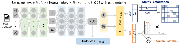
Figure 1. Overall architecture of our proposed method, SINN (Sociologically-Informed Neural Network).

4. Proposed method

In this work, we propose a deep learning framework, termed SINN (Sociologically-Informed Neural Network), for modeling and predicting the evolution of individuals’ opinions in a social network.

In this paper, inspired by recently developed physics-informed neural networks (Raissi et al., 2019b), we develop a deep learning framework that integrates both large-scale data from social media and prior scientific knowledge. Figure 1 shows the overall architecture of SINN. Opinion dynamics models, in their most common form, are expressed by difference equations (e.g., Equations (1) to (4)). We first reformulate these difference equations of opinion dynamics as ordinary differential equations (ODEs), which are shown in yellow in Figure 1. We then approximate the evolution of individuals’ opinions by a neural network (denoted by light blue). By penalizing the loss function with the ODEs, the neural network is informed by a system of ODEs that represent the opinion dynamics models; a concept drawn from theories of sociology and social psychology. The proposed framework is further combined with a language model (colored green in Figure 1) to fuse rich side information present in natural language texts (e.g., user profile descriptions). We also utilize low-rank approximation (dark blue) by factorizing the ODE parameters to capture the cluster structure of the social interaction network. The parameters of our model are trained via backpropagation.

Several opinion dynamics models involve stochastic processes, which encode random interactions between individuals. Stochastic sampling poses a challenge for end-to-end training because it would prevent the gradient of the loss from being back-propagated. In order to back-propagate through the stochastic variables, we leverage the reparametrization trick (orange in Figure 1) commonly used for gradient estimation (Kusner and Hernández-Lobato, 2016). This formulation makes the sampling process differentiable and hence the whole scheme can be trained in an end-to-end manner.

We elaborate the formulation of SINN in Section 4.1, followed by parameter learning in Section 4.2. The prediction and optimization procedure is presented in Appendix A.

4.1. Model Formulation

4.1.1. ODE constraint.

To incorporate social scientific knowledge, we rewrite opinion dynamics models as ordinary differential equations (ODEs). In the following, we formulate the ODEs by using some representative opinion dynamics models as guiding examples. Note though that our proposed framework can be generalized to any other opinion dynamics model. We use $\Lambda$ to denote the parameters of ODE.

DeGroot model. For the DeGroot model (DeGroot, 1974), we can transform the difference equation of Equation 1 into an ODE as follows:

(5) $$\frac{dx_{u}(t)}{dt}=\sum_{v\in\mathcal{U}\backslash u}a_{uv}x_{v}(t),$$

where $t$ is time and $x_{u}(t)$ is the user $u$’s latent opinion at time $t$. Higher values of $x_{u}(t)$ represent more positive opinions towards a given topic. Here we replace the discrete index $t$ (representing time step) of Equation 1 by the continuous variable $t$ (representing continuous time). The weight parameter, $a_{uv}$, indicates how much user $u$ is influenced by the opinion of user $v$. Equation 5 postulates that an individual’s opinion evolves over $t$ as a result of being influenced by the opinions of others. We can further modify Equation 5 to capture structural knowledge on social interaction (i.e., cluster structure). Real-world social networks have been found to contain multiple groups/communities of users sharing a common context (Kumar et al., 2006). To discover the cluster structure of the social interaction network, we apply matrix factorization to the matrix of weight parameter $A=\{a_{uv}\}\in\mathbb{R}^{U\times U}$. In particular, we factorize matrix $A$ into the two latent matrices of $M\in\mathbb{R}^{U\times K}$ and $Q\in\mathbb{R}^{U\times K}$: $A\approx M^{\top}Q$, where $K\ll U$ is the dimension of the latent space. Based on this parametrization, Equation 5 reduces to

(6) $$\frac{dx_{u}(t)}{dt}=\sum_{v\in\mathcal{U}\backslash u}\textbf{m}_{u}^{\top}\textbf{q}_{v}x_{v}(t),$$

where $\textbf{m}_{u}\in\mathbb{R}^{K}$ and $\textbf{q}_{v}\in\mathbb{R}^{K}$ correspond to the $u$-th column and $v$-th column of $M$ and $Q$. Equation 6 accounts for assimilation, a well-known phenomenon in social psychology.

Friedkin-Johnsen (FJ) model. For the FJ model (Friedkin and Johnsen, 1990), the difference equation of Equation 2 can be transferred into an ODE of the form:

(7) $$\frac{x_{u}(t)}{dt}=s_{u}\sum_{v\in\mathcal{U}\backslash u}x_{v}(t)+(1-s_{u})x_{u}(0)-x_{u}(t),$$

where $x_{u}(0)$ is the innate opinion of user $u$ at time $t=0$. In implementing this, we set the first expressed opinion of each user $u$ as the innate opinion $x_{u}(0)$. The interaction weight $a_{uv}$ denotes the influence user $u$ puts on $v$. The scaler parameter, $s_{u}\in[0,1]$, controls user $u$’s susceptibility to persuasion and so decides the degree of which the user is stubborn or open-minded.

Bounded confidence model (BCM). We transform the bounded confidence model of Hegselmann and Krause (Deffuant et al., 2000) into an ODE as follows. Since the original model function (Equation 3) is not differentiable, we replace the threshold function in Equation 3 with a sigmoid function. Formally,

(8) $$\frac{dx_{u}(t)}{dt}=\sum_{v\in\mathcal{U}}\sigma\big{(}\delta-|x_{u}(t)-x_{v}(t)|\big{)}\big{(}x_{v}(t)-x_{u}(t)\big{)},$$

where $\sigma(z)=(1+e^{-\gamma z})^{-1}$ denotes a sigmoid function. As the slope of sigmoid function $\gamma$ approaches infinity, Equation 8 will approach the thresholding function in the original model (Equation 3). This model choice draws on the theory of confirmation bias: Users tend to accept opinions that agree with theirs while discarding others. In Equation 8, if two users are close enough in their opinions (within confidence threshold $\delta$), they are likely to interact and develop a closer opinion; otherwise, they are not likely to interact, and maintain their original opinions.

Stochastic bounded confidence model (SBCM). The stochastic bounded confidence model (SBCM) involves sampling $z_{uv}^{t}\sim p(z_{uv}^{t})$ in Equation 4, which emulates stochastic interactions between users. Before triggering end-to-end training, we have to propagate the gradient through the non-differentiable sampling operation $\sim$ from a discrete distribution. Notice that as described in Section 4.1.2, latent opinion $x_{u}(t)$ is modeled by a neural network that involves a set of parameters to be optimized. To deal with the problem of the gradient flow block, we leverage the reparameterization approach. Using the Gumbel-Softmax trick (Jang et al., 2016), we can replace the discrete samples ${\bf z}_{u}^{t}=\{z_{u1}^{t},\ldots,z_{uU}^{t}\}$ with differentiable one-hot approximation $\tilde{\bf z}_{u}^{t}=\{\tilde{z}_{u1}^{t},\ldots,\tilde{z}_{uU}^{t}\}\in\mathbb{R}^{U}$ as follows:

(9) $$\tilde{\bf z}_{u}^{t}=\text{Softmax}\big{(}[\log{({\bf p}_{u}^{t})}+{\bf g}_{u}]/\tau\big{)},$$

where ${\bf p}_{u}^{t}\in\mathbb{R}^{U}$ consists of probability $p(z_{uv}^{t})$ for a set of users $v\in\mathcal{U}$ defined in Equation 4. ${\bf g}_{u}\in\mathbb{R}^{U}$ is the noise vector whose element is i.i.d and generated from the Gumbel distribution. This formulation allows randomness $\textbf{g}_{u}$ to be separated from the deterministic function of the parameters. In Equation 9, we relaxed the non-differentiable argmax operation to the continuous softmax function. $\tau$ is a temperature parameter controlling the degree of approximation; when $\tau\rightarrow 0$, the softmax function in Equation 9 approaches argmax and ${\bf z}_{u}^{t}$ becomes a one-hot vector. With the above formulation, we can propagate gradients to probabilities $p_{uv}^{t}$ through the sampling operation. Finally, SBCM is rewritten as

(10) $$\frac{dx_{u}(t)}{dt}=\sum_{v\in\mathcal{U}}\tilde{z}_{uv}^{t}\big{(}x_{v}(t)-x_{u}(t)\big{)}.$$

4.1.2. Neural network.

We then construct a neural network for approximating the evolution of individuals’ opinions. In this paper, we employ a feedforward neural network (i.e., FNN) with $L$ layers. The neural network takes time $t$ and user $u$ as inputs and outputs latent opinion $x_{u}(t)$ of user $u$ at that time, which is denoted by, $x_{u}(t)\approx f(t,{\bf e}_{u};\theta_{f})$, where $f(\cdot)$ represents the neural network, ${\bf e}_{u}$ is the one-hot encoding of a user index $u$, and $\theta_{f}$ represents the trainable parameters, namely, a set of weights and biases. We denote the output of neural network as $\hat{x}_{u}(t)=f(t,\textbf{e}_{u};\theta_{f})$. In our implementation, we adopt tanh activation for all layers. During training, we enforce the FNN output $\hat{x}_{u}(t)$ to (i) reproduce the observed opinions; and (ii) satisfy the governing ODEs that represent the theoretical models of opinion dynamics.

The FNN can be extended to incorporate rich side information. Here we assume that we are given individuals’ profile descriptions. To extract meaningful features from the profile descriptions, we adopt natural language processing techniques. We obtain hidden user representation $\textbf{h}_{u}=h(d^{u},\theta_{h})$, where $h(\cdot)$ is the language model, $d^{u}=\{w_{1}^{u},...,w_{|d^{u}|}^{u}\}$ is the sequence of words, $\theta_{h}$ is the trainable parameters. In this work, we adopt a pre-trained BERT Transformer (Devlin et al., 2018) as the language model and fine-tune an attention layer built on top of the pre-trained BERT model. The architecture of the language model is detailed in Section A.1. The hidden user representation is embedded into the FNN: $x_{u}(t)\approx f(t,\textbf{e}_{u},\textbf{h}_{u};\theta_{f})$. Although different types of additional information may be available, the above formulation focuses on user profile descriptions. Notice that our formulation is flexible enough to accept any new information. For example, the FNN can be further integrated with deep learning models to capture the influence of mass media (e.g., news websites) from their contents (e.g., news articles).

Table 1. Statistics of the three real-world datasets used in this paper.

	# Users	# Posts	# Positive	# Negative	# Classes	Time span
Twitter BLM	1,721	16,858	12,072	4,786	4	August 01, 2020 - March 31, 2021
Twitter Abortion	2,359	24,217	8,822	15,395	4	June 01, 2018 - April 30, 2021
Reddit Politics	1,335	22,563	5,724	16,839	2	April 30, 2020 - November 03, 2020

4.2. Parameter Learning

The proposed method, SINN, is trained to approximate the observations of opinions while satisfying the sociological and social psychological constraints determined by the ODEs. We aim to learn the neural network parameters $\theta_{f}$, the language model parameters $\theta_{h}$, as well as the ODE parameters $\Lambda$. The total loss $\mathcal{L}$ is thus composed of the data loss $\mathcal{L}_{\text{data}}$, the ODE loss $\mathcal{L}_{\text{ode}}$, and a regularization term, which is defined by

(11) $$\mathcal{L}(\theta_{f},\theta_{h},\Lambda;\mathcal{H},\mathcal{D})=\mathcal{L}_{\text{data}}(\theta_{f},\theta_{h};\mathcal{H},\mathcal{D})+\alpha\mathcal{L}_{\text{ode}}(\theta_{f},\theta_{h},\Lambda)+\beta\mathcal{R}(\Lambda),$$

where $\mathcal{L}_{\text{data}}$ measures the discrepancy between the labeled opinion and the neural network output. Meanwhile, $\mathcal{L}_{\text{ode}}$ measures the residual of ODEs, enforcing given sociological and social psychological constraints described by the ODEs. Hyperparameter $\alpha$ controls the balance between observed data $\mathcal{H}$ and prior scientific knowledge. $\mathcal{R}(\Lambda)$ is a regularization term and $\beta$ is the regularization parameter. In our experiment, the trade-off hyperparameters $\alpha$ and $\beta$ were chosen using grid search. We elaborate on each term of the loss function below.

Data Loss. The data loss term measures the deviation of predicted opinion $\hat{y}_{i}$ from ground truth opinion label $y_{i}$. We project latent opinion $\hat{x}_{u_{i}}(t_{i})$ of user $u_{i}$ at time $t_{i}$ to a probability distribution over opinion class labels by: $\hat{y}_{i}=\sigma(\hat{x}_{u_{i}}(t_{i})\textbf{w}_{\sigma}+\textbf{b}_{\sigma})$, where $\textbf{w}_{\sigma}\in\mathbb{R}^{C}$ is the scale parameter, $\textbf{b}_{\sigma}\in\mathbb{R}^{C}$ is the bias parameter, and $\sigma$ is a mapping function (softmax or sigmoid activation function for multi-class and two-class opinion labels, respectively). We adopt cross-entropy loss as the data loss to measure the difference between the predicted label distribution $\hat{y}_{i}$ with the truth label of opinion $y_{i}$:

(12) $$\mathcal{L}_{\text{data}}(\theta_{f},\theta_{h};\mathcal{H},\mathcal{D})=\frac{1}{I}\sum_{i=1}^{I}L_{\text{CE}}\big{(}\hat{y}_{i},y_{i}\big{)},$$

where $L_{\text{CE}}(\cdot)$ denotes cross-entropy loss. Equation 12 ensures that the neural network output coincides with the ground-truth opinion labels.

ODE Loss. This ODE loss enforces given scientific constraints as described by the ODEs (Equation 6, 7, 8, 9 and 10). To ensure the difference between the left side and right side of all ODEs are equal to zero, we minimize the mean squared error between them. Taking the DeGroot model in Equation 6 as example, ODE loss is written as

(13) $$\mathcal{L}_{\text{ode}}(\theta_{f},\theta_{h},\Lambda)=\frac{1}{J}\sum_{j=1}^{J}\sum_{u\in\mathcal{U}}\left(\left.\frac{d\hat{x}_{u}(t)}{dt}\right|_{t=\tau_{j}}-\sum_{v\in\mathcal{U}\backslash u}\textbf{w}_{u}^{\top}\textbf{h}_{v}\hat{x}_{v}(\tau_{j})\right)^{2},$$

where $\{\tau_{1},...,\tau_{J}\}$ is a set of $J$ collocation points. We randomly generate the collocation points from the time domain $\tau_{j}\in[0,T+\Delta T]$. $\mathcal{L}_{\text{ode}}$ measures the discrepancy of the ODEs at the $J$ collocation points, which ensures that the neural network output satisfies the ODE constraints. The first derivative term $\frac{d\hat{x}_{u}(t)}{dt}$ in Equation 13 can be easily computed using automatic differentiation (Baydin et al., 2018) in deep learning packages such as PyTorch (Paszke et al., 2017).

Regularizer. We can use auxiliary constraints as the regularization term $\mathcal{R}(\cdot)$ in Equation 11. For DeGroot model, to prevent over-fitting, we add the following regularization on the latent matrices: $\mathcal{R}(\Lambda)=\|M\|_{1}+\|Q\|_{1}$, where $\|M\|_{1}$ denotes the $l_{1}$-norm of the latent matrix $M$.

The parameter optimization is described in Section A.2.

5. Experiments

We conduct qualitative and quantitative experiments to evaluate the performance of the proposed method, SINN (Sociology-Informed Neural Network), on both synthetic and real-world datasets. In this section, we present our experimental settings and results. Our source code and sample data are publicly available.

5.1. Datasets

Experiments were conducted on three synthetic datasets of different settings and three real-world datasets collected from Twitter and Reddit. The data preprocessing procedure is detailed in Section B.1.

5.1.1. Synthetic datasets.

We generate synthetic datasets using the stochastic bounded confidence model (SBCM). We simulate the following three scenarios created with three different exponent parameters $\rho$ of the SBCM in Equation 4: i) Consensus ($\rho=-1.0$), ii) Polarization ($\rho=0.5$), and iii) Clustering ($\rho=0.05$). The bottom panel of Figure 2 shows the simulated opinion evolution for the Consensus dataset. Our simulation involves $U=200$ users whose initial opinions are uniformly distributed. All simulations were run for $T=200$ timesteps. For a fair comparison, we converted the simulated continuous opinion values into five discrete labels and used these labels as the input of the models. Please refer to Section B.1.1 for details.

5.1.2. Real datasets.

We use two Twitter datasets and one Reddit dataset. Table 1 shows the statistics of the three real-world datasets.

Twitter datasets. We construct two Twitter datasets by collecting tweets related to specific topics, i.e., BLM (BlackLivesMatter) and Abortion, through the Twitter public API using hashtags and keywords. For BLM, we crawled tweets containing hashtag #BlackLivesMatter from August 1, 2020, to March 31, 2021. For Abortion dataset, tweets were extracted between June 1, 2018, and April 30, 2021, using hashtag #Abortion. Each tweet contains date/time, user, and text. To remove bots, and spam users, we filtered the set of users based on the usernames and the number of posts. The preprocessing procedure is presented in Section B.1.2. All tweets are manually annotated into highly positive, positive, negative, highly negative towards the corresponding topic. Along with the tweets, we obtained the profile descriptions (i.e., the user-defined texts describing their Twitter accounts) for all the users. For each user, the profile description is represented as a collection of words.

Reddit datasets. For Reddit dataset, we collect posts from two Reddit communities (i.e., subreddits) for political discussion: r/libertarian and r/conservative. All submissions were retrieved through the Pushshift API from April through November 2020, and include date/time, user, and subreddit. Users with less than five posts and more than 1,000 posts were discarded, leaving 1,335 users. We label posts in r/libertarian 0 (negative towards conservatism) and r/conservative 1 (positive).

5.2. Comparison methods

We compare the prediction performance of SINN with the following baselines:

• Voter (Voter model) (Yildiz et al., 2010): Voter is one of the simplest models of opinion dynamics. At each time step, users select one of the users uniformly at random and copy her opinion.

• DeGroot (DeGroot model) (DeGroot, 1974): DeGroot is a classical opinion dynamics model; it assumes users update their opinions iteratively to the weighted average of the others’ opinions. We analytically solve Equation 5 and fit the model parameter $a_{uv}$.

• AsLM (Asynchronous Linear Model) (De et al., 2014): AsLM is a linear regression model where each opinion is regressed on the previous opinions.

• SLANT (De et al., 2016): SLANT is a temporal point process model that captures the influence of the other users’ opinions. It characterizes a self-exciting mechanism of the interaction between users and its time decay is based on intensity.

• SLANT+ (Kulkarni et al., 2017): SLANT+ is an extension of SLANT, which combines recurrent neural network (RNN) with a point process model. RNN learns the non-linear evolution of users’ opinions over time.

• NN: NN is the proposed method without ODE loss $\mathcal{L}_{\text{ode}}$ in Equation 11, in which the trade-off hyperparameters are fixed to $\alpha=0$ and $\beta=0$.

Detailed settings for the baselines are specified in Section B.2.

5.3. Experimental Setup

5.3.1. Evaluation Protocol.

For each synthetic dataset, we split the training, validation, and test set in a proportion of 50%, 20%, 30% in chronological order. We divide each real-world dataset into train, validation, and test set with ratios of 70%, 10%, and 20%. To evaluate the prediction performance of all models, we measure the accuracy (ACC) and the macro F1 score (F1), both of which assess the agreement between predicted opinion classes and the ground truth.

5.3.2. Hyperparameters.

Hyperparameters of all methods, including comparison methods and ours, are tuned by grid search on the validation set. For the neural network models, we determine the number of layers $L$ in the range of $\{3,5,7\}$ and the hidden layer dimension in the range of $\{8,12,16\}$. For our SINN, we search in $\{0.1,1.0,5.0\}$ for the trade-off hyperparameters $\alpha$ and $\beta$; $\{1,2,3\}$ is taken as the dimension of the latent space $K$. We test four opinion dynamics models (Equations (6) to (10)) and report the results of the best one. We selected the pre-trained $\text{BERT}_{\text{BASE–uncased}}$ as the language model of our SINN (See Section B.3 for the detailed setting). We use the Adam optimizer (Kingma and Ba, 2014) with learning rate 0.001 for all experiments.

Table 2. F1 score (F1) and Accuracy (ACC) for predicting opinions from three synthetic datasets. Higher scores indicate better prediction performance. The best performance is highlighted in bold.

	Consensus		Polarization		Clustering
	ACC	F1	ACC	F1	ACC	F1
Voter	0.457	0.197	0.248	0.204	0.274	0.202
DeGroot	0.458	0.260	0.706	0.515	0.765	0.524
AsLM	0.155	0.264	0.113	0.079	0.477	0.325
SLANT	0.006	0.002	0.038	0.025	0.190	0.064
SLANT+	0.008	0.003	0.113	0.041	0.386	0.111
NN	0.771	0.426	0.603	0.451	0.875	0.817
Proposed	0.794	0.574	0.761	0.738	0.895	0.843

Table 3. F1 score (F1) and Accuracy (ACC) for predicting opinions from three real-world datasets. Higher is better. The best performance is highlighted in bold.

	Twitter BLM		Twitter Abortion		Reddit Politics
	ACC	F1	ACC	F1	ACC	F1
Voter	0.199	0.163	0.222	0.170	0.628	0.500
DeGroot	0.203	0.131	0.358	0.203	0.807	0.389
AsLM	0.092	0.117	0.435	0.195	0.789	0.441
SLANT	0.105	0.070	0.425	0.175	0.733	0.496
SLANT+	0.091	0.042	0.437	0.152	0.789	0.441
NN	0.336	0.237	0.441	0.369	0.875	0.824
Proposed	0.359	0.246	0.467	0.412	0.927	0.884

5.4. Quantitative Evaluation

We first report the prediction performance of different methods in terms of the two evaluation metrics on the three synthetic datasets in Table 2. We can observe that the proposed SINN achieves the best results in terms of accuracy (ACC) and F1 score (F1). None of the comparison methods perform robustly across all datasets. AsLM achieves the second best F1 score among the baselines for the Consensus dataset but fails on the Polarization and Clustering datasets. DeGroot outperforms the other baseline methods on the Polarization dataset, while providing relatively poor performance for the Consensus and Clustering datasets. It is due to the fact that they depend on the specific choice of opinion dynamics model used. In contrast, SINN is general and suits different opinion dynamics models, which yields better performance in all experiments. In an additional experiment (Section B.4.2), we demonstrated that SINN can be used to select one of a set of opinion dynamics models that best captures hidden social interaction underlying data.

Table 3 shows the results of the existing methods and SINN on three real-world datasets. SINN achieves the best prediction performance in all cases. AsLM gives almost the worst performance for Twitter BLM dataset. This is because AsLM is a linear model and cannot adequately depict the complex interaction between users. SLANT and SLANT+ have less predictive power since they assume a fixed parametric form for social interaction. Compared with these methods, deep learning-based models (i.e., NN and SINN) offer improved performance in terms of accuracy and F1 score. The reason is that the deep learning-based models can learn the complex mechanisms of opinion formation in real-world social networks due to the influence of external factors (e.g., mass media) and random behavior, which are not considered in the other methods. Importantly, SINN yields better prediction performance than NN across all the datasets. Compared with NN, SINN achieves 11.7% improvement in terms of F1 for Twitter Abortion dataset. For Reddit dataset, it produces a result of 88.4% in F1, which is an 7.3% improvement over NN. This result verifies the effectiveness of incorporating prior scientific knowledge into the deep learning model, as well as the advantage of our model design. From these results, we can conclude that SINN can learn from both data and theoretical models. We perform a parameter study in Section B.4.1.

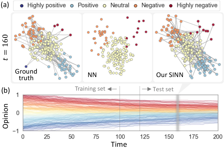
Figure 2. (a) Interactions between users at time $t=160$, which is simulated (left) and predicted by NN (middle) and SINN (right). Nodes represent users where the color indicates their opinion classes. The left graph illustrates the true social interactions during $t\in[160,170]$. The middle graph shows the opinion classes predicted by NN. The right graph visualizes the opinion classes and the interaction parameter $\tilde{z}_{uv}^{t}$ of SBCM (Equation 10) learned by SINN. (b) Temporal evolution of individuals’ opinions simulated in Consensus dataset. Each curve represents one individual.

5.5. Qualitative Evaluation via Case Studies

Figure 2 depicts the temporal changes in population opinions and the networks of social interactions for the Consensus dataset. In the Consensus dataset, the population reaches consensus (Figure 2(b)) through social interactions between users with opposite opinions (Figure 2(a) left). We can see in Figure 2(a) that SINN (right) can duplicate the actual interactions that frequently occur between opposing users (left). As can be seen from the node colors, SINN (right) better captures the actual opinion dynamics (left) than NN (middle). In NN, a large number of negative samples (light blue nodes) are mislabeled as neutral ones (yellow). SINN, however, misclassifies only a few negative samples as neutral. This result validates the benefit of incorporating prior sociological and social psychological knowledge in the form of the ODEs.

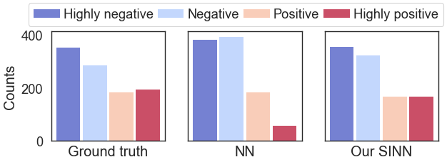
Figure 3. Distribution of opinion classes on November 7, 2020 for Twitter Abortion dataset.

Figure 3 compares the distribution of opinion classes for Twitter Abortion dataset. For comparison, we show actual and predicted class distributions on November 7, 2020. We can see that SINN better reproduces the ground-truth label distribution than NN. On the other hand, NN underestimates the number of highly negative samples (red bar). This further emphasizes the importance of using prior knowledge and the effectiveness of our approach.

Figure 4 visualizes the most important words in the profile descriptions identified by the attention mechanisms in NN and SINN for Twitter Abortion dataset. As shown in this figure, NN tends to focus on meaningless or general words (e.g., ’https’, ’co’, ’year’), while SINN selects words (e.g., ’Pro’(-Life/Choice), ’Freedom’, ’Liberty’) that are more relevant to the given topic (i.e., Abortion). With the help of prior scientific knowledge, SINN can extract meaningful features from rich side information like textual descriptions to better predict opinion evolution. To save space, we only report the results from one dataset in Figures 2, 3 and 4.

6. Conclusion and Future work

In this paper, we tackle the problem of modeling and predicting opinion dynamics in social networks. We develop a novel method that integrates sociological and social psychological knowledge and a data-driven framework, which is referred to as SINN (Sociologically-Informed Neural Network). Our approach is the first attempt to introduce the idea of physics-informed neural networks into opinion dynamics modeling. Specifically, we first reformulate opinion dynamics models into ordinary differential equations (ODEs). For stochastic opinion dynamics models, we apply the reparameterization trick to enable end-to-end training. Then we approximate opinion values by a neural network and train the neural network approximation under the constraints of the ODE. The proposed framework is integrated with matrix factorization and a language model to incorporate rich side information (e.g., user profiles) and structural knowledge (e.g., cluster structure of the social interaction network). We conduct extensive experiments on three synthetic and three real-world datasets from social networks. The experimental results demonstrate that the proposed method outperforms six baselines in predicting opinion dynamics.

For future work, we try to integrate an opinion mining method (Medhat et al., 2014) into our framework to automatically obtain opinion labels for social media posts. This avoids expensive annotations. We also plan to explore other side information such as mass media contents (e.g., news articles) and social graphs (e.g., follow/following relationship). Furthermore, although this paper focuses on four representative opinion dynamics models, our framework can be generalized for any opinion dynamics model.

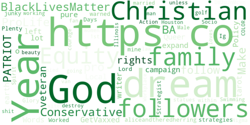
(a) NN

(b) Our SINN

Figure 4. Important words in profile descriptions identified by attention mechanisms in (a) NN and (b) SINN for Twitter Abortion dataset.

Supplemental Material

Appendix A Proposed method

A.1. Language Model

The language model $h(\cdot,\theta_{h})$ takes as input profile description $d^{u}$, and infers the hidden user representation $\textbf{h}_{u}$. User profile description $d^{u}$ consists of a sequence of $|d^{u}|$ words $d^{u}=\{w_{1}^{u},...,w_{|d^{u}|}^{u}\}$. Input sentence $d^{u}$ is first padded to a fixed length of $N$ words with NULL tokens $d^{u}=\{w_{1}^{u},...,w_{N}^{u}\}$ and tokenized. We pick 25 as the max sentence length (i.e., profile description) $N$. Original sentences with over $N=25$ words are truncated at the end. This truncation would not significantly affect the final result, because the most of profile descriptions contain no more than 25 words. 91% of users in the Twitter BLM dataset have less than 25 words ($|d^{u}|<25$) in their profile descriptions; likewise 89% of users in the Twitter Abortion dataset. In this work, we select a pre-trained BERT Transformer (Devlin et al., 2018) as the language model. The input tokens $d^{u}=\{w_{1}^{u},...,w_{N}^{u}\}$ are mapped into a sequence of $b$-dimensional word vectors $\{{\bf w}_{1}^{u},...,{\bf w}_{N}^{u}\}$ through the pre-trained BERT model. We add an attention layer on top of the last hidden layer of the frozen pre-trained BERT to learn the importance of each word in the sentence. Our attention layer takes as input the word vectors ${\bf w}_{n}^{u}$, and calculates the attention score for each vector: $e_{n}={\bf w}_{n}^{\top}{\bf E}$, where $\textbf{E}\in\mathbb{R}^{b}$ is the context vector. The corresponding attention weight is defined as $\tilde{e}_{n}=\exp{(e_{n})}/\sum_{n^{\prime}}\exp{(e_{n^{\prime}})}$. To compute the hidden representation of user $u$, we compute the weighted average of the word embeddings of each word in the profile description: $\textbf{h}_{u}=\sum_{n=1}^{N}\tilde{e}_{n}{\bf w}_{n}^{u}$.

A.2. Optimization

We solve the following minimization problem to find optimal parameters of neural network $\theta_{f}$, language model $\theta_{h}$ and the ODEs $\Lambda$:

(14) $$\theta_{f}^{\ast},\theta_{h}^{\ast},\Lambda^{\ast}=\mathop{\rm arg~{}min}\limits_{\{\theta_{f},\theta_{h},{\bf\Lambda}\}}\,\,\,\mathcal{L}(\theta_{f},\theta_{h},\Lambda;\mathcal{H},\mathcal{D}),$$

where $\{\theta_{f}^{\ast},\theta_{h}^{\ast},\Lambda^{\ast}\}$ denote the optimal set of parameters. The loss function can be minimized by using a backpropagation algorithm. For the stochastic bounded confidence model (SBCM), during the backward pass, we can obtain the gradient of the discrete sample by computing the gradient of our continuous approximation $\tilde{\bf z}_{u}^{t}$ in Equation 9. This allows the model to be optimized in an end-to-end manner.

A.3. Preidiction

During the test phase, we use the trained neural network to predict the future opinion $y^{\ast}$ of user $u^{\ast}$ at time $t^{\ast}$. The opinion can be predicted by calculating the hidden representation $\textbf{h}_{u^{\ast}}$ of user $u^{\ast}$, and feeding it into the trained neural network: $y^{\ast}=f(t^{\ast},\textbf{e}_{u^{\ast}},\textbf{h}_{u^{\ast}};\theta_{f}^{\ast})$, where $\textbf{e}_{u^{\ast}}$ is the one-hot encoding of user $u^{\ast}$.

Appendix B Experiment

B.1. Datasets

Experiments were conducted on three synthetic datasets and three real-world datasets.

B.1.1. Synthetic dataset

We generated the syntetic datasets using the SBCM (stochastic opinion dynamics model) in Equation 3 and 4. We consider a social network with a set of $U=200$ users. For each dataset, the model was run for $T=200$ consecutive timesteps, resulting in a total of $I=40,000$ data points. At the first timestamp, initial opinions are randomly drawn from a uniform distribution between 0 and 1. In each timestep from 2 to 200, we randomly choose 15 users who initiate interaction with other users. When individual $u$ initiates an interaction, a partner $v$ is selected from a set of $U=200$ users with probability $p_{uv}^{t}$ defined by Equation 4. User $u$ then updates her opinion $x_{u}(t+1)$ at time $t+1$ by weighted averaging her own opinion $x_{u}(t)$ and the chosen partner’s opinion $x_{v}(t)$ at time $t$:

(15) $$x_{u}(t+1)=x_{u}(t)+\mu x_{v}(t),$$

where parameter $\mu$ indicates the strength of influence. We set $\mu=0.1$ in all the simulations. The three datasets differ in the exponent parameter $\rho$ that reach different final states: $\rho=-1.0$ (opinion consensus), $\rho=0.1$ (opinion clustering), and $\rho=1.0$ (opinion polarization). Finally, we divided the continuous opinion value into five classes according to the range as highly negative ($-1.0\text{--}-0.6$), negative ($-0.6\text{--}-0.2$), neutral ($-0.2\text{--}0.2$), positive ($0.2\text{--}0.6$), and highly positive ($0.6\text{--}1.0$) and used these class labels as the input of the models.

B.1.2. Twitter datasets

We used Twitter API to collect English tweets posted by Twitter users, specific to BLM and Abortion. The replies and retweets are not included in these datasets. All the tweets were pre-processed before annotation. First, we excluded the URLs, usernames (@user), and email addresses from the original tweets. To remove corporate accounts, bot accounts, and spammers, we excluded users who tweeted more than 30,000 tweets in total and less than three tweets, and those that contain the words “bot” and “news” in their username. To filter news tweets, we also excluded the tweet that contained specific keywords (i.e., ’news’, ’call’, ’tell’, ’say’, ’announce’, ’state’, ’country’, ’city’, ’council’). Moreover, we eliminated duplicate tweets. Annotators classified them into one of the following opinion classes: highly negative, negative, neutral, positive, highly positive, and not applicable. The “not applicable” label means the annotator could not make any judgment. Tweets with “not applicable” label were removed from the dataset. We also eliminated the tweets with “neutral” label since many of them contain only irrelevant information. The human-annotated labels are considered as the ground truth and the performance of the models is calculated with respect to these labels.

Twitter profile descriptions are preprocessed as follows: (i) removing URLs, usernames and email addresses, (ii) eliminating stop words (“the”, “is”, “an” etc.), (iii) remove extra white space, special characters, (iv) lowercasing, and (v) tokenization. We employed the BERT basic tokenizer (See Section B.3).

B.1.3. Reddit dataset

The Reddit dataset was drawn from social media platform Reddit. Using the Reddit API, we collected a total of 70,876 Reddit posts between April 30th and November 3rd, 2020. We focus on two major communities (subreddits) discussing conservative and libertarian politics: r/conservative and r/libertarian. The dataset included anonymous user IDs and subreddits, as well as timestamps. We preserved only those users who had between 5 and 1,000 posts, which resulted in a set of 1,335 users. We assign label 0 (negative to conservative) to each post if it belongs to r/libertarian, label 1 (positive) if it belongs to r/conservative.

B.2. Comparison methods

In this subsection, we describe the settings for the baselines.

Some existing methods (i.e., Voter and AsLM) are designed for time series data observed at regular time intervals. To compare these methods, we treat the most recent opinion value as the one at the previous time step.

Moreover, as the four baselines of DeGroot, AsLM, SLANT, and SLANT+ can handle only continuous opinion values rather than discrete class labels, we transform discrete opinion labels to continuous values in $[-1,1]$ using linear scaling. At the time of evaluation, we rescale the predicted opinion values back to the discrete opinion labels, by grouping them into sets of discrete labels according to the range as highly negative ($-1.0\text{--}-0.6$), negative ($-0.6\text{--}-0.2$), neutral ($-0.2\text{--}0.2$), positive ($0.2\text{--}0.6$), and highly positive ($0.6\text{--}1.0$).

Since SLANT and SLANT+ are primarily intended for predicting the opinion of the next post, we predict the long-term evolution of individuals’ opinions during the future time window by iteratively predicting the next post. The predicted opinion values are used as the input of the next time step. This procedure is repeated until time $T+\Delta T$.

B.3. Implementation details

All code was implemented using Python 3.9 and PyTorch (Paszke et al., 2017). We conducted all experiments on a machine with four 2.8GHz Intel Cores and 16GB memory. For the neural networks (i.e., NN, the FNN of our SINN), we used the same number of hidden units $N_{u}$ in all hidden layers. For the language model of SINN, we used the tokenizer and pre-trained BERT from the Python library pytorch-pretrained-bert. The hidden size of $\text{BERT}_{\text{BASE–uncased}}$ is set to 768. The input dimension of the attention layer was 768 and the output dimension was equal to the number of hidden units $N_{u}$ of the FNN $f(\cdot)$. The model parameters were trained using the ADAM optimizer (Kingma and Ba, 2014) with $\beta_{1}=0.9$, $\beta_{2}=0.999$ and a learning rate of 0.001. By default, we set 128 as the mini-batch size, 1000 as the number of epochs, and $J=1$ as the number of collocation points.

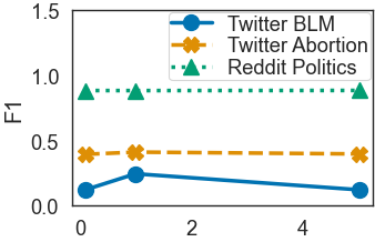
(a) Trade-off parameter $\alpha$

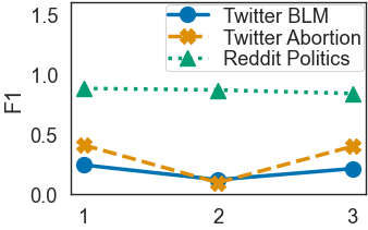
(b) Dimension of latent space $K$

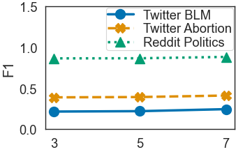
(c) number of layers $l$

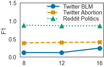
(d) Number of units $N_{u}$

Figure 5. Prediction performance with different values of hyperparameters using F1 score.

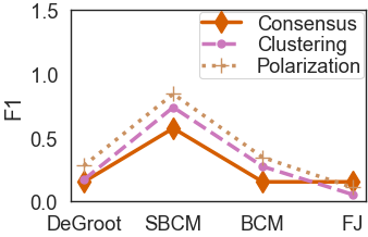
(a) Synthetic datasets

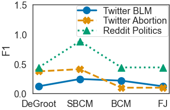
(b) Real-world datasets

Figure 6. Prediction performance with different opinion dynamics models using F1 score.

B.4. Additional Results

B.4.1. Sensitivity Analysis

We investigate the sensitivity of SINN on the core hyperparameters. Due to space limitations, we present only the results on the real-world datasets in Figure 5.

Figure 5(a) shows the prediction performance (in terms of F1) by varying the trade-off hyperparameter $\alpha$ in Equation 11. SINN achieves the best performance when $\alpha=1.0$ for all the real-world datasets.

In Figure 5(b), we vary the dimension of latent space $K$. Our SINN gives the best results when $K=1$ for Twitter BLM dataset and Reddit Politics dataset; and $K=3$ for Twitter Abortion dataset.

In Figures 5(c) and 5(d), we show the impact of neural network architecture by varying the number of layers $L$ and units $N_{u}$ in the neural network. We can observe that SINN yields robust performance with respect to the size of the neural network (i.e., the number of layers $L$ and the number of units per layer $N_{u}$).

We also evaluate the importance of side information (i.e., user profiles) by comparing SINN with and without profile descriptions. For Twitter Abortion dataset, the use of such information improves the F1 score by 10.2%. Meanwhile, it does not show improvement in prediction accuracy for Twitter BLM dataset. In future work, we will explore different choices of the language model.

B.4.2. Impact of Opinion Dynamics Models

We evaluate different choices of opinion dynamics models on prediction performance. Figure 6 reports the F1 results of SINN with four different opinion dynamics models: DeGroot model, FJ model, bounded confidence model (BCM), stochastic opinion dynamics model (SBCM). For all the synthetic datasets, the SBCM outperforms all other opinion dynamics models explored in this study. That is, SINN successfully identifies the original opinion dynamics model that generated the synthetic datasets (i.e., SBCM) from a set of candidates. SINN also gives the best results on the SBCM for the real-world datasets. It suggests the importance of considering the stochastic nature of social interaction.

References

- (1)
- Abelson (1964) Robert P Abelson. 1964. Mathematical models of the distribution of attitudes under controversy. Contributions to mathematical psychology (1964).
- Acemoğlu et al. (2013) Daron Acemoğlu, Giacomo Como, Fabio Fagnani, and Asuman Ozdaglar. 2013. Opinion fluctuations and disagreement in social networks. Mathematics of Operations Research 38, 1 (2013), 1–27.
- Baumann et al. (2021) Fabian Baumann et al. 2021. Emergence of polarized ideological opinions in multidimensional topic spaces. Physical Review X 11, 1 (2021), 011012.
- Baydin et al. (2018) Atilim Gunes Baydin et al. 2018. Automatic differentiation in machine learning: A survey. Journal of machine learning research 18 (2018).
- Chen et al. (2020) Yuyao Chen, Lu Lu, George Em Karniadakis, and Luca Dal Negro. 2020. Physics-informed neural networks for inverse problems in nano-optics and metamaterials. Optics express 28, 8 (2020), 11618–11633.
- Como and Fagnani (2009) Giacomo Como and Fabio Fagnani. 2009. Scaling limits for continuous opinion dynamics systems. In 47th Annual Allerton Conference on Communication, Control, and Computing. IEEE, 1562–1566.
- De et al. (2014) Abir De et al. 2014. Learning a Linear Influence Model from Transient Opinion Dynamics. In Proceedings of the 23rd CIKM. ACM, 401–410.
- De et al. (2016) Abir De et al. 2016. Learning and Forecasting Opinion Dynamics in Social Networks. In Proceedings of the 30th NeurIPS. 397–405.
- Deffuant et al. (2000) Guillaume Deffuant, David Neau, Frédéric Amblard, and Gérard Weisbuch. 2000. Mixing beliefs among interacting agents. Advances in Complex Systems 3, 1-4 (2000), 87–98.
- DeGroot (1974) Morris H DeGroot. 1974. Reaching a consensus. J. Amer. Statist. Assoc. 69, 345 (1974), 118–121.
- Devi and Kamalakkannan (2020) G Dharani Devi and S Kamalakkannan. 2020. Literature Review on Sentiment Analysis in Social Media: Open Challenges toward Applications. International journal of Advanced Science and Technology 29, 7 (2020), 1462–1471.
- Devlin et al. (2018) Jacob Devlin, Ming-Wei Chang, Kenton Lee, and Kristina Toutanova. 2018. Bert: Pre-training of deep bidirectional transformers for language understanding. arXiv preprint arXiv:1810.04805 (2018).
- Eirinaki et al. (2013) Magdalini Eirinaki, Malamati D Louta, and Iraklis Varlamis. 2013. A trust-aware system for personalized user recommendations in social networks. IEEE transactions on systems, man, and cybernetics: systems 44, 4 (2013), 409–421.
- French Jr (1956) John RP French Jr. 1956. A formal theory of social power. Psychological review 63, 3 (1956), 181.
- Friedkin and Johnsen (1990) Noah E Friedkin and Eugene C Johnsen. 1990. Social influence and opinions. Journal of Mathematical Sociology 15, 3-4 (1990), 193–206.
- Galam (1999) Serge Galam. 1999. Application of statistical physics to politics. Physica A: Statistical mechanics and its applications 274, 1-2 (1999), 132–139.
- Golub and Jackson (2012) Benjamin Golub and Matthew O Jackson. 2012. How homophily affects the speed of learning and best-response dynamics. The Quarterly Journal of Economics 127, 3 (2012), 1287–1338.
- Hegselmann and Krause (2002) Rainer Hegselmann and Ulrich Krause. 2002. Opinion dynamics and bounded confidence: Models, analysis and simulation. J. Artif. Soc. Soc. Simul. 5, 3 (2002).
- Jager and Amblard (2005) Wander Jager and Frédéric Amblard. 2005. Uniformity, bipolarization and pluriformity captured as generic stylized behavior with an agent-based simulation model of attitude change. Computational & Mathematical Organization Theory 10, 4 (2005), 295–303.
- Jang et al. (2016) Eric Jang, Shixiang Gu, and Ben Poole. 2016. Categorical reparameterization with gumbel-softmax. arXiv preprint arXiv:1611.01144 (2016).
- Kingma and Ba (2014) Diederik P Kingma and Jimmy Ba. 2014. Adam: A method for stochastic optimization. arXiv preprint arXiv:1412.6980 (2014).
- Kulkarni et al. (2017) Bhushan Kulkarni et al. 2017. SLANT+: A Nonlinear Model for Opinion Dynamics in Social Networks. In Proceedings of the 17th ICDM. IEEE Computer Society, 931–936.
- Kumar et al. (2018) Naveen Kumar, Deepak Venugopal, Liangfei Qiu, and Subodha Kumar. 2018. Detecting review manipulation on online platforms with hierarchical supervised learning. Journal of Management Information Systems 35, 1 (2018), 350–380.
- Kumar et al. (2006) Ravi Kumar, Jasmine Novak, and Andrew Tomkins. 2006. Structure and evolution of online social networks. In Proceedings of the 12th KDD. ACM, 611–617.
- Kusner and Hernández-Lobato (2016) Matt J Kusner and José Miguel Hernández-Lobato. 2016. GANs for sequences of discrete elements with the gumbel-softmax distribution. arXiv preprint arXiv:1611.04051 (2016).
- Lai et al. (2018) Mirko Lai, Viviana Patti, Giancarlo Ruffo, and Paolo Rosso. 2018. Stance Evolution and Twitter Interactions in an Italian Political Debate (Lecture Notes in Computer Science, Vol. 10859). Springer, 15–27.
- Lanchier (2012) Nicolas Lanchier. 2012. The Axelrod model for the dissemination of culture revisited. The Annals of Applied Probability 22, 2 (2012), 860–880.
- Leshem and Scaglione (2018) Amir Leshem and Anna Scaglione. 2018. The impact of random actions on opinion dynamics. IEEE Transactions on Signal and Information Processing over Networks 4, 3 (2018), 576–584.
- Liu and Wang (2013) Qipeng Liu and Xiaofan Wang. 2013. Social learning with bounded confidence and probabilistic neighbors. In Proceedings of the IEEE International Symposium on Circuits and Systems. IEEE, 2303–2306.
- Martins (2008) André CR Martins. 2008. Continuous opinions and discrete actions in opinion dynamics problems. International Journal of Modern Physics C 19, 04 (2008), 617–624.
- Medhat et al. (2014) Walaa Medhat, Ahmed Hassan, and Hoda Korashy. 2014. Sentiment analysis algorithms and applications: A survey. Ain Shams engineering journal 5, 4 (2014), 1093–1113.
- Monti et al. (2020) Corrado Monti, Gianmarco De Francisci Morales, and Francesco Bonchi. 2020. Learning Opinion Dynamics From Social Traces. In Proceedings of the 26th KDD. ACM, 764–773.
- Moussaïd et al. (2013) Mehdi Moussaïd, Juliane E Kämmer, Pantelis P Analytis, and Hansjörg Neth. 2013. Social influence and the collective dynamics of opinion formation. PloS one 8, 11 (2013), e78433.
- O’Connor et al. (2010) Brendan O’Connor et al. 2010. From Tweets to Polls: Linking Text Sentiment to Public Opinion Time Series. In Proceedings of the 4th ICWSM. The AAAI Press.
- Paszke et al. (2017) Adam Paszke et al. 2017. Automatic differentiation in pytorch. (2017).
- Raissi et al. (2019a) Maziar Raissi et al. 2019a. Deep learning of vortex-induced vibrations. Journal of Fluid Mechanics 861 (2019), 119–137.
- Raissi et al. (2019b) Maziar Raissi, Paris Perdikaris, and George E Karniadakis. 2019b. Physics-informed neural networks: A deep learning framework for solving forward and inverse problems involving nonlinear partial differential equations. J. Comput. Phys. 378 (2019), 686–707.
- Ranade et al. (2019) Rishikesh Ranade, Sultan Alqahtani, Aamir Farooq, and Tarek Echekki. 2019. An extended hybrid chemistry framework for complex hydrocarbon fuels. Fuel 251 (2019), 276–284.
- Sánchez-Núñez et al. (2020) Pablo Sánchez-Núñez et al. 2020. Opinion Mining, Sentiment Analysis and Emotion Understanding in Advertising: A Bibliometric Analysis. IEEE Access 8 (2020), 134563–134576.
- Schweighofer et al. (2020) Simon Schweighofer, David Garcia, and Frank Schweitzer. 2020. An agent-based model of multi-dimensional opinion dynamics and opinion alignment. Chaos: An Interdisciplinary Journal of Nonlinear Science 30, 9 (2020), 093139.
- Sobkowicz (2016) Pawel Sobkowicz. 2016. Quantitative agent based model of opinion dynamics: Polish elections of 2015. PloS one 11, 5 (2016), e0155098.
- Sun et al. (2020) Luning Sun, Han Gao, Shaowu Pan, and Jian-Xun Wang. 2020. Surrogate modeling for fluid flows based on physics-constrained deep learning without simulation data. Computer Methods in Applied Mechanics and Engineering 361 (2020), 112732.
- Sun and Müller (2013) Zhanli Sun and Daniel Müller. 2013. A framework for modeling payments for ecosystem services with agent-based models, Bayesian belief networks and opinion dynamics models. Environmental modelling & software 45 (2013), 15–28.
- Sznajd-Weron and Sznajd (2000) Katarzyna Sznajd-Weron and Jozef Sznajd. 2000. Opinion evolution in closed community. International Journal of Modern Physics C 11, 06 (2000), 1157–1165.
- Taylor (1968) Michael Taylor. 1968. Towards a mathematical theory of influence and attitude change. Human Relations 21, 2 (1968), 121–139.
- Yang et al. (2020) Liu Yang et al. 2020. Physics-informed generative adversarial networks for stochastic differential equations. SIAM Journal on Scientific Computing 42, 1 (2020), A292–A317.
- Yildiz et al. (2010) Mehmet Ercan Yildiz et al. 2010. Voting models in random networks. In Information Theory and Applications Workshop (ITA). IEEE, 419–425.
- Zhang et al. (2019) Dongkun Zhang, Lu Lu, Ling Guo, and George Em Karniadakis. 2019. Quantifying total uncertainty in physics-informed neural networks for solving forward and inverse stochastic problems. J. Comput. Phys. 397 (2019), 108850.
- Zhang and Hong (2013) Jiangbo Zhang and Yiguang Hong. 2013. Opinion evolution analysis for short-range and long-range Deffuant–Weisbuch models. Physica A: Statistical Mechanics and its Applications 392, 21 (2013), 5289–5297.
- Zhang et al. (2017) YunHong Zhang, QiPeng Liu, and SiYing Zhang. 2017. Opinion formation with time-varying bounded confidence. PloS one 12, 3 (2017), e0172982.
- Zhu et al. (2020) Lixing Zhu, Yulan He, and Deyu Zhou. 2020. Neural opinion dynamics model for the prediction of user-level stance dynamics. Information Processing & Management 57, 2 (2020), 102031.