Predicting binding energies of astrochemically relevant molecules via machine learning

Abstract

Context. The behaviour of molecules in space is to a large extent governed by where they freeze out or sublimate. The molecular binding energy is thus an important parameter for many astrochemical studies. This parameter is usually determined with time-consuming experiments, computationally expensive quantum chemical calculations, or the inexpensive, but inaccurate, linear addition method.

Aims. In this work we propose a new method based on machine learning for predicting binding energies that is accurate, yet computationally inexpensive.

Methods. A machine learning model based on Gaussian Process Regression is created and trained on a database of binding energies of molecules collected from laboratory experiments presented in the literature. The molecules in the database are categorized by their features, such as mono- or multilayer coverage, binding surface, functional groups, valence electrons, and H-bond acceptors and donors.

Results. The performance of the model is assessed with five-fold and leave-one-molecule-out cross validation. Predictions are generally accurate, with differences between predicted and literature binding energies values of less than $\pm$20%. The validated model is used to predict the binding energies of twenty one molecules that have recently been detected in the interstellar medium, but for which binding energy values are not known. A simplified model is used to visualize where the snowlines of these molecules would be located in a protoplanetary disk.

Conclusions. This work demonstrates that machine learning can be employed to accurately and rapidly predict binding energies of molecules. Machine learning complements current laboratory experiments and quantum chemical computational studies. The predicted binding energies will find use in the modelling of astrochemical and planet-forming environments.

1 Introduction

One of the objectives of the field of astrochemistry is to understand the formation, destruction, and survival of molecules in astrophysical environments, such as star-forming regions or planet-forming disks (Jørgensen et al., 2020; Öberg & Bergin, 2021). This concerns, for instance, the molecular reactions on dust-grain surfaces, where the surface acts as a catalyst (Cuppen et al., 2017) and evaporation of ices in hot cores near young massive stars (Viti et al., 2004). To model such phenomena certain molecule-specific parameters are needed. Both examples require a measure of how strongly the molecule binds to the surface, that is the binding energy (BE). In astrophysical environments physisorption is the primary source of the BE. The main contributors of physisorption are van der Waals forces, which arises from dipole-dipole interactions, and hydrogen bonding between the adsorbed molecule and surface. These forces act at a distance between 2-4 $\mathrm{\SIUnitSymbolAngstrom}$. If no dynamical barrier is present, the BE is equal to the activation energy of desorption ($E_{\mathrm{des}}$) as the system reference energy (i.e., $E$ = 0) corresponds to the adsorbed molecule and surface at infinite separation Minissale et al. (2022).

Experimentally, a prominent technique to determine the BE is by temperature programmed desorption (TPD). This applies to studies of catalysis (Luo et al., 1997), surface science (Zhou et al., 2007), as well as astrochemistry (Muñoz Caro et al., 2010). The TPD process consists of three steps; first, the molecule is adsorbed to the surface at cold temperatures. The coverage may be below or above a single monolayer depending on various factors such as the molecular flux and deposition time. If more molecules than available surface adsorption sites are deposited, the coverage is also termed multilayer. Second, the temperature is linearly increased, resulting in desorption of molecules at specific temperatures. Third, the desorbed molecules are detected, often with a mass spectrometer. This produces spectra of desorption rate as a function of temperature. The process of thermal desorption is generally described by the Polanyi-Wigner equation, a modified Arrhenius law:

$$-\frac{dN}{dt}=k_{\rm des}(T)\cdot N^{\rm n},$$ (1)

$$-\frac{dN}{dt}=\nu_{\rm n}\cdot N^{\rm n}\cdot{\rm exp}\left(-\frac{E_{\rm des}}{k_{\rm B}\cdot T}\right),$$ (2)

where  $k_{\rm des}(T)$ is the desorption rate constant in s^-1 at temperature $T$, $N$ the number of adsorbed molecules on a surface, $n$ the order of desorption (usually 1 for monolayer desorption and 0 for multilayer desorption), $\nu_{\rm n}$ the pre-exponential frequency factor with value molecules^1-n s^-1 (also often denoted as $A$), $E_{\rm des}$ the desorption energy and $k_{\rm B}$ the Boltzmann constant. For a more thorough discussion of the technique and analysis, we refer to De Jong & Niemantsverdriet (1990), Burke & Brown (2010), and Minissale et al. (2022) for contextual reviews.

While TPD has been successful in determining the BEs for many molecules that are of astrochemical relevance (e.g., Brown & Bolina, 2007; Burke et al., 2015a; Smith & Kay, 2018; Behmard et al., 2019; Salter et al., 2019), there are limitations to experimental BE investigations with this and other techniques. Experiments are time-consuming and the focus usually is on the scientifically most impactful systems. With the vast number of known interstellar molecules, this inevitably means that some of them are not yet studied. Furthermore, certain molecular species are difficult to work with, either because they are unstable or highly reactive (e.g., vinyl alcohol, cyanopolyynes), highly toxic (e.g., methyl isocyanate, propyl cyanide), or simply challenging to produce an ice film with (e.g, carbamide).

Alternatively, Bayesian inference (Heyl et al., 2022) or quantum chemical computational methods can be used to determine BEs (e.g., Das et al., 2018; Rimola et al., 2018; Balbisi et al., 2022). Quantum chemical calculation can also take into account BE distributions on amorphous and highly anisotropic surfaces (e.g., Tinacci et al., 2022; Ferrero et al., 2020; Duflot et al., 2021). However, since these methods are computationally expensive, many astrochemical studies rely on the so-called linear addition method. With this method, the BE of a molecule is determined by splitting its components in atoms and molecular fragments for which the BEs are known and subsequently adding them together (e.g., Garrod & Herbst, 2006; Shingledecker et al., 2020). This method is computationally inexpensive, but it is also inaccurate. Novel methods that are computationally inexpensive, but more accurate are required.

Machine learning (ML) has become one of the most prominent scientific tools of the $21^{\mathrm{st}}$ century as it provides high accuracy at low computational cost. It has the ability to handle and interpret data in ways impossible to humans, which allows for the discovery of unprecedented patterns (Jordan & Mitchell, 2015). These properties make ML an interesting alternative to the above-mentioned theory-based approaches. With immense versatility ML has applications ranging from self-driving cars and social media to banking and image recognition. In recent years, ML has also made its entrance as a powerful tool in astrochemistry and astrophysics. Notable deployments include Lee et al. (2021) for reproducing and predicting chemical abundances in interstellar inventories and Shallue & Vanderburg (2018) for exoplanet identification. Another type of ML models are ML interatomic potentials, which can be directly employed as low-cost alternatives to quantum chemical calculations for investigating for example molecular reactivity, adsorption and diffusion on dust grains (e.g., Mazo-Sevillano et al., 2021; Molpeceres, G. et al., 2021; Zaverkin et al., 2021). In surface science and catalysis, ML has also been used extensively to identify predictive models for BEs (e.g., Gu et al., 2020; Fung et al., 2021; Andersen & Reuter, 2021).

In this work, we apply supervised ML to a data set of BEs obtained from literature TPD data and thereby develop a model to predict BEs between new molecules and surfaces relevant to astrochemical environments. The methods used are discussed in Sect. 2. The results and discussion of the analysis are presented in Sect. 3. Astrophysical implications are covered in Sect. 4 and the conclusions of this work are given in Sect. 5.

2 Methods and data

Supervised learning algorithms are constructed to make a model that can recognise particular patterns within the data when given training examples by the user (supervisor). A strong limitation of such algorithms is that they can only recognise data that are related to the training data, therefore, any anomaly or unseen data structures would be difficult for the model to grasp. The training data given to the model in our work is a data set of BEs obtained from TPD experiments collected from the literature as well as relevant features of each system such as the surface category and atoms and functional groups present in the adsorbed molecule. Hence, the trained model can be expected to predict BEs for new examples of molecules and surfaces that are not too different from those seen in the training data. We quantify the predictive accuracy of our model by carrying out two types of cross validation analysis. The workflow of the process is shown in Fig. 1. In the following sections, the essential components of this workflow are described.

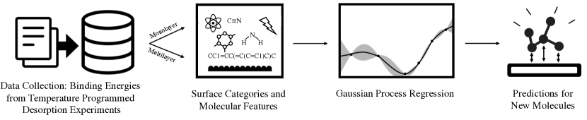
Figure 1: Schematic overview of the workflow. First the data is collected from the literature and divided into monolayer and multilayer coverage. Secondly, specific features are designated to the data, including atomic composition, functional groups and valence electrons. Thirdly, the Gaussian Process Regression model is constructed and trained on the data to be able to predict BEs for new molecules.

2.1 Gaussian process regression

BEs are here predicted using the supervised ML technique Gaussian Process Regression (GPR). It is a probabilistic, non-parametric supervised learning method frequently used for regression and classification problems in the ML community. Being based on Bayesian probability theory, it learns a posterior probability distribution over all admissible target functions. Here, these are functions describing the relationship between surface/molecular features (the input $x$) and the TPD BE (the output $y$). A Gaussian Process prior is assumed, which means that both the prior and posterior probability distributions are Gaussian distributed (normal) and can be specified using a mean function, $\mu(x)$, and a covariance function, $k(x,x^{\prime})$, also called the kernel function. The posterior distribution is calculated by conditioning the prior distribution on the training data set. Model predictions on new test data points with input $x_{*}$ are obtained from the mean of the posterior distribution, $\mathbf{\bar{f}}_{*}$, given by

$$\mathbf{\bar{f}}_{*}=\boldsymbol{\mu_{*}}+k(x_{*},x)[k(x,x)+{\sigma_{n}^{2}}I]^{-1}(\mathbf{y}-\boldsymbol{\mu})\quad,$$ (3)

and variances are obtained from the diagonal of the covariance matrix, ${\rm cov}(\mathbf{f}_{*})$, given by

$${\rm cov}(\mathbf{f}_{*})=k(x_{*},x_{*})-k(x_{*},x)[k(x,x)+{\sigma_{n}^{2}}I]^{-1}k(x,x_{*})\quad.$$ (4)

Here $\boldsymbol{\mu}$ and $\boldsymbol{\mu_{*}}$ are the mean vectors, $k(x,x_{*})$ denotes the covariance matrix evaluated at all pairs of training and test points, and similarly for the other entries $k(x,x)$, $k(x_{*},x_{*})$ and $k(x_{*},x)$. The target function is assumed to be noisy, which is accounted for by the incorporation of independently, identically distributed Gaussian noise, $\sigma_{n}^{2}I$. In practise, a small or vanishing noise level will cause the fitted model to follow the training data points closely, whereas a higher noise level will result in a smoother model. The latter can be useful for extrapolating to unseen data since more emphasis is put on trends rather than the individual training examples seen. The variance provides an uncertainty estimate, that is how confident we can be about the model predictions, and it is also affected by the noise level. The direct access to an uncertainty estimate is a great advantage of GPR compared to other types of ML methods such as neural networks (Scalia et al., 2020).

GPR belongs to the class of kernelized ML methods that employ internally the “kernel trick”. A kernel is a function that corresponds to an inner product in some high-dimensional feature space, whose values can be interpreted as a similarity measure of input data points. In this way, the kernel function implicitly maps the inputs into a higher dimensional space and applies the linear algorithm there, which is the basic idea how kernelized ML methods tackle the computational complexity of dealing with high-dimensional feature spaces. We refer to Rasmussen & Williams (2006) for an extensive textbook coverage of GPR and to Gibson et al. (2012)) and Aigrain et al. (2012) for examples of GPR applied to exoplanet data sets.

For the actual GPR implementation, we rely in this work on the ML library Scikit-learn (Pedregosa et al., 2011), which provides a number of built-in kernels. By testing several different combinations of kernels using five-fold cross validation (cf. Sect. 3.1), we found that the best performance is achieved by using the sum of the radial basis function (RBF) kernel

$$k_{\mathrm{RBF}}(\textbf{x}_{i},\textbf{x}_{j})=\exp{\left[-\frac{1}{2\ell_{1}^{2}}(\textbf{x}_{i}-\textbf{x}_{j})^{2}\right]}$$ (5)

and the rational quadratic (RQ) kernel

$$k_{\mathrm{RQ}}(\textbf{x}_{i},\textbf{x}_{j})=\exp{\left[1+\frac{(\textbf{x}_{i}-\textbf{x}_{j})^{2}}{2\alpha\ell_{2}^{2}}\right]}^{-\alpha}\quad.$$ (6)

The length-scale parameters, $\ell_{1}$ and $\ell_{2}$, indicate how quickly the correlation between two points drops as their distance increases. A higher $\ell$ gives a smoother function and a smaller $\ell$ gives a wigglier function (Rasmussen & Williams, 2006). $\alpha$ determines the relative weighting of large-scale and small-scale variations in the RQ kernel (Duvenaud, 2014). $\ell_{1}$, $\ell_{2}$ and $\alpha$, along with the noise level from Eq. 3 and 4, are hyperparameters. Here we determine these parameters during the model training by maximising the marginal likelihood function using the standard Limited-memory Broyden-Fletcher-Goldfarb-Shanno algorithm for bound-constrained optimization (L-BFGS-B) Byrd et al. (1995); Zhu et al. (1997).

2.2 Data set and features

We have compiled the training data by analysing laboratory studies presented in the literature and extracting the relevant information. From these publications, BEs determined with TPD experiments and information about the binding surface are retrieved, which resulted in a data set that initially contained 354 (167) entries for the monolayer (multilayer) case and 117 different molecules, many of which have been detected in the interstellar medium. They range from simple diatomics like N₂ and CO, organic molecules like ethanol (CH₃CH₂OH) and glycolaldehyde (HOCH₂CHO), long carbon chains such as octane (C₈H₁₈), and biomolecules like the nucleobase adenine.

Besides the BEs, the training data set also contains input features, which are descriptive attributes of the surfaces and molecules. It is essential to choose the best possible features as they govern how well the model predicts; too few features and the model will not be able to differentiate between different training data points (e.g. molecules), and too many features could invoke the curse of dimensionality, which is a term expressing how increasing the volume of feature space dilutes the data (Bellman, 1966). Therefore, the best approach is to minimise the number of features while maximising the amount of information they contain.

In this work, molecular features, such as atomic compositions (C, H, O, N, Cl) and functional groups (alcohol, –OH; carbonyl, –C(O)–; carboxyl, –COOH; ester, –C(O)O–; ether, –O–; amine, –NH₂; cyanide, –CN; amide, –NC(O)–), are used. Several features are obtained from the python module RDkit (Landrum, 2020). These are calculated by converting the molecules to SMILES strings, which are then fed into RDkit. The considered features are the number of valence electrons, hydrogen bond donors, hydrogen bond acceptors, and topological polar surface area (TPSA). The latter is a property defined as the molecule’s sum of surface area of polar atoms and is measured in Ų. The motivation for applying the features from RDkit is to try to encapsulate the origin of the dominating forces that govern the binding of molecules. This includes in particular hydrogen bonding and van der Waals interactions. Finally, we also included the molecular mass and the number of atoms in the molecule as features. An overview of all molecular features used is given in Table LABEL:tab:features and a selection of the feature values of each molecule are presented in Table LABEL:tab:molecule_features.

Table 1: Overview of the features used to describe the molecules and surfaces.

Atoms	Functional Groups	RDKit & Misc.	Surface	Examples of surface
Carbon	Alcohol i (–OH)	Number of H-bond acceptors	Carbon	Graphene, graphite and
Chlorine	Amide iii (–NC(O)–)	Number of H-bond donors		highly orientated pyrolytic graphite
Hydrogen	Amine iii (–NH2)	Number of valence electrons	Metal	Gold and nickel
Nitrogen	Carbonyl (–C(O)–)	Topological polar surface area
Oxygen	Carboxyl (–COOH)		Silicate	Amorphous silicate and forsterite
	Cyanide — (–CN)	Mass
	Ester iiiii (–C(O)O–)	Number of atoms	Water	Amorphous solid water and
	Ether i——ii (–O–)			crystalline water

For the consideration of features related to the surface, we first divide our data set into two categories; monolayer and multilayer coverage. Entries recorded at monolayer coverage (that is, an adsorbate layer of one molecule thickness) or less are assumed to have their BE dominated by the surface-molecule interaction. A wide variety of different surfaces are present in the analysed literature, the number of which greatly exceeds what is reasonable for the model to handle. To reduce this, the surfaces are placed in four different sub-categories based on their common traits. The categories and their main contributors annotated with the percentage they comprise of the total entries in the category are the following: Carbon (graphene, graphite and highly orientated pyrolytic graphite, 94 % of data entries), metal (gold, 56 % of data entries), silicate (amorphous silicate and forsterite, 93 % of data entries) and water (amorphous solid water and crystalline water, 98 % of data entries). We note that this approximation could be a source of significant noise in the training data, as different types of surfaces here placed in the same category (e.g. nickel and gold for metals) may in reality bind the studied molecules with different strength, however, they cannot be distinguished from the used input features. Finally, in order to input the surface category feature to the ML algorithm it is converted to numerical values using one hot encoding.

For multilayer entries, the coverage is greater than one molecule in thickness and the BE is assumed to be dominated by intermolecular interactions of the adsorbed species with itself. For this reason, we have chosen to neglect surface features for the multilayer data set.

Finally, we note that, while for further analysis only the BE is used, it is important to be aware of the influence of the pre-exponential factor. This value can be experimentally determined, but often (including in many of the studies that contribute to the data set in this work) an assumed value is used in the analysis to retrieve the BE. Compared to an experimentally determined pre-exponential factor, the assumed value may result in significantly deviating BEs and their inclusion in the training data will affect the results of the ML model. It is also worth noting that adsorbates on amorphous and highly anisotropic surfaces usually have a distribution of BEs rather than a single value (Shimonishi et al., 2018). However, since the available TPD data mainly consists of a single binding energy per surface/molecule combination, this distribution is presently not possible to include in our model.

2.3 Data preparation

Since ML algorithms generally do not perform well on data points that are rare or very different from the remaining of the data set, we combed our data set for outliers. This was done by applying the ‘isolation forest algorithm’ from Scikit-learn (Pedregosa et al., 2011). It identifies anomalies that are both few in numbers and different in feature space. The isolation forest has been applied in both the mono- and multilayer case. It resulted in removal of three outliers for both cases: the C₆₀ fullerene and the two polycyclic aromatic hydrocarbons (PAHs) coronene and ovalene. For the multilayer case we also removed two other molecules (dotriacontane and guanine) since these molecules, together with the fullerene and the PAHs, are outliers in the sense that they have BEs that are 3-4 times as large as the other molecules in the data set.

Lastly, we addressed the issue that data points with the same feature representation can have different labels (BEs). This can arise when several different experimental measurements of the same surface/molecule combination are present in the data set, which differ only in experimental parameters that in our model have been assumed not to influence the BE, such as temperature ramp, starting temperature and pre-exponential factor. In this case an average over the measured BEs are used. If, on the other hand, this issue arises due to differences in parameters such as the initial coverage and the specific surface (for the monolayer data set), a more thoughtful approach is fruitful. If data points at both sub-monolayer and monolayer coverage are present, we use the monolayer data point since the sub-monolayer case may be dominated by specific surface sites exhibiting a more favourable (stronger) binding than the others. If data points for several specific surfaces or facets are present within the same surface category, we use the surface that occurs most frequently within the category in order to get a more coherent data set. After this data preparation step, the final data set contains 143 (46), entries for the monolayer (multilayer) case and 114 individual molecules. After the data preparation step the features were normalised to have zero mean and unit variance, with the exception of the one-hot-encoded surface features. This is a standard procedure in the ML community to make the learning task easier. All data points used in this work, their actual surface and assigned surface category are given in Table LABEL:tab:monolayer_data and LABEL:tab:multilayer_data for monolayer and multilayer coverage species, respectively.

3 Results and discussion

In the following sections we validate the performance of the model using two different types of assessment; five-fold cross validation and leave-one-molecule-out cross validation.

3.1 Five-fold cross validation

Five-fold cross validation is a standard approach in the ML community for comparing models and for assessing how well they can predict new data points. As illustrated in Fig. 5 in Appendix A, it is carried out by splitting the data set into five disjoint equally sized sets. The model is then trained on four of the sets while the fifth set is used to validate the model (i.e. by comparing model predicted BEs to actual BEs). This is repeated five times until every data point has been used as validation data exactly once. In Fig. 2 we show parity plots of ML predictions on the combined validation data set from the five folds versus actual literature BEs for the monolayer and multilayer data sets. The closer the points are to the diagonal dotted line, the better the model performs. The performance is quantified using the root-mean-square error (RMSE) and more absolutely by the coefficient of determination, $R^{2}$.

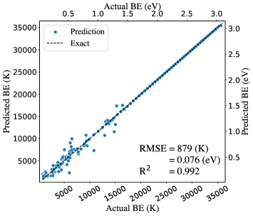
(a) Monolayer

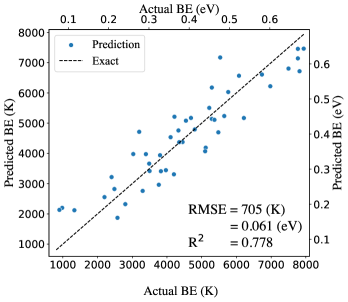
(b) Multilayer

Figure 2: Parity plots for a) monolayer and b) multilayer coverage comparing ML-predicted BEs against actual BEs for the combined validation set from five-fold cross validation.

It is found that the model has the highest $R^{2}$ value for the monolayer case shown in Fig. 2a. One contributor to this could be the fact that there are more than three times as many entries for the monolayer set than for the multilayer set. However, a much more important difference between the two data sets is that for the monolayer case the model is exceptionally accurate for data points with a BE above 17000 K. The reason for this behaviour is that this part of the data set is immensely uniform as it consists only of carbohydrate chains of varying lengths adsorbed on graphene surfaces. Since the BE increases proportionally with the length of the carbon chain, the model is able to learn these BEs with a very high accuracy. In fact, if only the entries with BE above 17000 K are included in the analysis, the model achieves a RMSE of 25.7 K and an $R^{2}$ value of approximately one. This RMSE is much lower than the overall RMSE of 879 K, especially when taken into consideration that the scale of the data set is higher. However, it should be kept in mind that the model is only as nuanced as the data it has been provided. This implies that the model has a very narrow knowledge of molecules in the high BE regime, and thus the predictive capability would most likely be limited for molecules different from the simple carbohydrates. If only the low energy regime is considered, the $R^{2}$ value decreases to 0.946. The corresponding parity plot, Fig. 6, can be found in the appendix.

3.2 Leave-one-molecule-out cross validation

As a second type of assessment, we next evaluate how well the model can predict individual new molecules. This is done by first removing a chosen molecule from the data set (including all surface categories for the monolayer case), then training the model on the reduced data set, and finally comparing the ML-predicted BE of the chosen molecule with the literature value. For this assessment eight different molecules have been chosen, namely acetone ($\mathrm{CH}_{3}\mathrm{C(O)CH}_{3}$), acetonitrile ($\mathrm{CH}_{3}\mathrm{CN}$), allyl alcohol ($\mathrm{C}_{3}\mathrm{H}_{5}\mathrm{OH}$), ammonia ($\mathrm{NH}_{3}$), methane ($\mathrm{CH}_{4}$), methylformate ($\mathrm{CH}_{3}\mathrm{OCHO}$), the alkane nonacosane ($\mathrm{C}_{29}\mathrm{H}_{60}$) and the nucleobase thymine ($\mathrm{C}_{5}\mathrm{H}_{6}\mathrm{N}_{2}\mathrm{O}_{2}$), which represent diverse chemical compositions and molecular sizes.

The comparison between ML-predicted and actual BEs are shown in table LABEL:tab:predictnew. The model uncertainty estimates are obtained from the standard deviation of the posterior distribution (i.e. the square root of its variance), as described in Sect. 2.1. As seen, the overall predictive capability of the model is reasonably good. Furthermore, there is a direct correlation between how well different types of molecules are represented in the training data and how well the model predicts them. For example, it is found that nonacosane is exactly predicted, which is presumably a consequence of the many similar molecules in the data set. It is further noticeable that ammonia is predicted quite reasonably, even though the model is mostly trained on organic molecules. We can identify that the good prediction accuracy mainly comes from the inclusion of the following molecular features; number of valence electrons, H-bond acceptors, H-bond donors and TPSA, since the predicted BE for a monolayer of ammonia on a carbon surface is only $2070\pm 1740$ K (a deviation of $-31$ % compared to the literature value) if these features are excluded. For the multilayer case the deviation would be even more pronounced at $-36$ %. The model struggles the most with allyl alcohol, acetontrile and methyl formate, although the deviations are still relatively small at $\pm$ $\sim$20 %. This might be because the training data set contains few molecules like these three or because another factor such as the specific surface has an influence on the BE, which the model cannot account for.

Table 2: Comparison between ML-predicted and literature BE values (rounded to the nearest ten) for leave-one-molecule-out cross validation.

Name	Molecule	Surface or Coverage	Prediction	Literature	Deviation
			(K)	(K)
Acetone	$\mathrm{CH}_{3}\mathrm{C(O)CH}_{3}$	Water	ii 4520 $\pm$ ii450 ii	i 4690 $\pm$ 240	$-3.6$ %
Acetonitrile	$\mathrm{CH}_{3}\mathrm{CN}$	Metal	ii 6730 $\pm$ ii880 ii	i 5530 $\pm$ 360	$21$ %
Allyl alcohol	$\mathrm{C}_{3}\mathrm{H}_{5}\mathrm{OH}$	Metal	ii 7110 $\pm$ 1740 ii	6010† iiiii	$18$ %
Ammonia	$\mathrm{NH}_{3}$	Carbon	$2870\pm 1700$	i 2990 $\pm$ 240	$-4.0$ %
Methane	$\mathrm{CH}_{4}$	Carbon	ii 1870 $\pm$ ii470 ii	i 1700 $\pm$ 120	$10$ %
Methyl formate	$\mathrm{CH}_{3}\mathrm{OCHO}$	Water	ii 5390 $\pm$ ii540 ii	i 4510 $\pm$ 530	$19$ %
Nonacosane	$\mathrm{C}_{29}\mathrm{H}_{60}$	Carbon	i 23720 $\pm$ i 220 iii	23720 $\pm$ 930	$0.0$ %
Thymine	$\mathrm{C}_{5}\mathrm{H}_{6}\mathrm{N}_{2}\mathrm{O}_{2}$	Metal	$11680\pm 2600$ i	12930 $\pm$ 240	$-9.6$ %
Acetonitrile	$\mathrm{CH}_{3}\mathrm{CN}$	Multilayer	ii 4030 $\pm$ ii470 ii	i 4800 $\pm$ 190	$-16$ %
Ammonia	$\mathrm{NH}_{3}$	Multilayer	ii 3330 $\pm$ ii960 ii	i 3030 $\pm$ 240	$9.9$ %
Methyl formate	$\mathrm{CH}_{3}\mathrm{OCHO}$	Multilayer	ii 4520 $\pm$ ii470 ii	i 4110 $\pm$ 200	$10$ %

We also recall here that some types of molecules are not well represented in the training data, meaning that the developed model is not suitable for predicting these. This concerns foremost the types of molecules that were removed as outliers in the data preparation step (fullerenes, PAHs, and large aromatic molecules in general). Also phenols are notoriously difficult to perform TPD experiments with, and therefore not much data is available for the model to train on.

In general, a further limitation of the developed model is that it cannot distinguish between isomers of the same molecule, in the case these have the same feature representation, which will always be the case for structural isomers. However, given the other uncertainties - both in the experimental TPD procedure and in the developed model - it is very likely that the difference in BE between two isomers would anyway be much smaller than what can be resolved with the current approach.

Another limitation of the model is that it struggles with molecules consisting of atoms other than C, H, O, N and Cl. This is because the data set includes very few molecules that contain other than said atoms and because we consequently do not include features representing any other atoms. This means that predicting the BEs of for example sulphurous- and phosphorous-containing molecules will be less accurate. To increase the performance and predictive capabilities of the model, the most essential future step would be to increase and diversify the number of entries in the training data set.

4 Astrophysical implications

Table 3: Predictions of BEs for molecules with astrophysical relevance measured in K and rounded to nearest 10.

Name	Molecule	Surface	Prediction	Prediction	Estimate
			(K)	(eV)	(K)
Cyanamide	NH2CN	Carbon	$8780\pm 3730$	$0.76\pm 0.32$	5556a
Cyanamide	NH2CN	Water	$8730\pm 3710$	$0.75\pm 0.32$
Ethanimine	CH3CHNH	Carbon	$4350\pm 1100$	$0.37\pm 0.09$	5580b
Ethanimine	CH3CHNH	Water	$4010\pm 1620$	$0.35\pm 0.14$
Vinylalcohol	CH2CHOH	Carbon	6000 $\pm$ i 260	$0.52\pm 0.02$	–
Vinylalcohol	CH2CHOH	Water	5910 $\pm$ i 400	$0.51\pm 0.03$	–
Propargylimine	HC3HNH	Carbon	$4580\pm 1210$	$0.40\pm 0.10$	14750c
Propargylimine	HC3HNH	Water	$4260\pm 1630$	$0.37\pm 0.14$
Cyanomethanimine	HNCHCN	Carbon	$6670\pm 2110$	$0.57\pm 0.18$	10900c
Cyanomethanimine	HNCHCN	Water	$6750\pm 2100$	$0.58\pm 0.18$
Methyl isocyanate	CH3NCO	Carbon	$3360\pm 1440$	$0.29\pm 0.12$	6486d
Methyl isocyanate	CH3NCO	Water	$2990\pm 1490$	$0.26\pm 0.13$
Acetamide	CH3C(O)NH2	Carbon	8420 $\pm$ i 520	$0.73\pm 0.04$	–
Acetamide	CH3C(O)NH2	Water	8350 $\pm$ i 530	$0.72\pm 0.04$	–
N-Methylformamide	CH3NHCHO	Carbon	$7920\pm 1290$	$0.68\pm 0.11$	7386d
N-Methylformamide	CH3NHCHO	Water	$7880\pm 1340$	$0.68\pm 0.11$
Carbamide / Urea	NH2C(O)NH2	Carbon	$11930\pm 4350$ i	$1.02\pm 0.37$	–
Carbamide / Urea	NH2C(O)NH2	Water	$11960\pm 4350$ i	$1.03\pm 0.37$	–
Ethenediol	HOCHCHOH	Carbon	$9130\pm 3230$	$0.79\pm 0.28$	–
Ethenediol	HOCHCHOH	Water	$8840\pm 3240$	$0.76\pm 0.28$	–
Ethanolamine	HOCH2CH2NH2	Carbon	8550 $\pm$ 2250	0.74 $\pm$ 0.19	–
Ethanolamine	HOCH2CH2NH2	Water	8380 $\pm$ 2260	0.72 $\pm$ 0.19	–
Allenyl acetylene	H2CCCHCCH	Carbon	4360 $\pm$ i 370	$0.37\pm 0.03$	–
Allenyl acetylene	H2CCCHCCH	Water	5120 $\pm$ i 320	$0.44\pm 0.03$	–
Propargyl cyanide†	HCCCH2CN	Carbon	6840 $\pm$ i 650	$0.59\pm 0.05$	18750c
Propargyl cyanide†	HCCCH2CN	Water	9520 $\pm$ i 310	$0.82\pm 0.03$
Cyanoallene†	CH2CCHCN	Carbon	6840 $\pm$ i 650	$0.59\pm 0.06$	–
Cyanoallene†	CH2CCHCN	Water	9520 $\pm$ i 310	$0.82\pm 0.03$	–
Cyanopropyne†	CH3C3N	Carbon	6840 $\pm$ i 650	$0.59\pm 0.06$	–
Cyanopropyne†	CH3C3N	Water	9520 $\pm$ i 310	$0.82\pm 0.03$	–
n-Propylcyanide‡	CH3CH2CH2CN	Carbon	7320 $\pm$ i 850	$0.63\pm 0.07$	21350c
n-Propylcyanide‡	CH3CH2CH2CN	Water	9650 $\pm$ i 680	$0.83\pm 0.06$
i-Propylcyanide‡	CH3CH(CN)CH3	Carbon	7320 $\pm$ i 850	$0.63\pm 0.08$	–
i-Propylcyanide‡	CH3CH(CN)CH3	Water	9650 $\pm$ i 680	$0.83\pm 0.07$	–
Hydroxyacetone	CH3C(O)CH2OH	Carbon	$6560\pm 3800$	$0.57\pm 0.33$	–
Hydroxyacetone	CH3C(O)CH2OH	Water	$6510\pm 3660$	$0.56\pm 0.31$	–
Cyanovinylacetylene*	HCCCHCHCN	Carbon	7430 $\pm$ i 860	$0.63\pm 0.07$	22600c
Cyanovinylacetylene*	HCCCHCHCN	Water	10850 $\pm$ i 340 i	$0.93\pm 0.03$
Vinylcyanoacetylene*	H2CCHC3N	Carbon	7430 $\pm$ i 860	$0.63\pm 0.07$	–
Vinylcyanoacetylene*	H2CCHC3N	Water	10850 $\pm$ i 340 i	$0.93\pm 0.03$	–
Methylcyanodiacetylene	CH3C5N	Carbon	$7900\pm 1000$	$0.68\pm 0.09$	7880c
Methylcyanodiacetylene	CH3C5N	Water	11540 $\pm$ i 480 i	$0.99\pm 0.04$
Cyanoacetyleneallene	H2CCCHC3N	Carbon	8120 $\pm$ 1050	0.70 $\pm$ 0.09	26750c
Cyanoacetyleneallene	H2CCCHC3N	Water	11700 $\pm$ i 570 i	1.01 $\pm$ 0.05
1-cyano-1,3-cyclopentadiene	c-C5H5CN	Carbon	$8260\pm 1100$	$0.71\pm 0.09$	–
1-cyano-1,3-cyclopentadiene	c-C5H5CN	Water	11270 $\pm$ i 790 i	$0.97\pm 0.07$	–
Cyanotriacetylene	HC7N	Carbon	$8360\pm 1130$	$0.72\pm 0.10$	7780c
Cyanotriacetylene	HC7N	Water	12040 $\pm$ i 630 i	$1.04\pm 0.05$
Cyanotetraacetylene	HC9N	Carbon	$9490\pm 1320$	$0.82\pm 0.11$	9380c
Cyanotetraacetylene	HC9N	Water	$12420\pm 1020$ i	$1.07\pm 0.09$
Cyanopentaacetylene	HC11N	Carbon	$10600\pm 1460$ i	$0.91\pm 0.12$	10980c
Cyanopentaacetylene	HC11N	Water	$12820\pm 1260$ i	$1.10\pm 0.11$
Indene	c-C9H8	Carbon	8930 $\pm$ i 230	$0.77\pm 0.02$	–
Indene	c-C9H8	Water	6300 $\pm$ i 890	$0.54\pm 0.08$	–

In recent years, the number of newly detected molecules in the interstellar medium has skyrocketed, including many complex organic molecules and prebiotic species such as carbamide (NH₂C(O)NH₂, Belloche et al., 2019), propargylimine (HC₃HNH, Bizzocchi et al., 2020), propargyl cyanide (HCCCH2CN, McGuire et al., 2020), ethanolamine (HOCH₂CH₂NH₂, Rivilla et al., 2021), and allenyl acetylene (H₂CCCHCCH, Cernicharo et al., 2021). While these detections underline the molecular complexity that is present in star-forming regions, a limited knowledge of fundamental physicochemical parameters such as reaction rate constants, photo destruction cross sections, and BEs prevents us from fully understanding how these species form, react, respond to physical conditions, and, ultimately, what their place is in the interstellar chemical factory.

In this section we first employ the ML model to predict the BEs of a number of molecules that have been detected in the interstellar medium, but for which no or limited information about their BEs can be found in the literature, see Table LABEL:tab:astro_species. The features of the molecules are encoded in the same way as the training data for the ML model and presented in Table LABEL:tab:astro_species_features. Predictions of BEs for monolayer coverage are limited to two surfaces, carbon and water, for which the model shows the highest performance. For a number of species, BE estimates based on the linear addition method are available in the literature and have been used in modelling studies. These BEs are generic, meaning that they are not specific to any surface. These literature estimates are included in Table LABEL:tab:astro_species for comparison to our ML predictions.

Several observations are made for the predicted BEs. The uncertainties on the predictions vary from a few % to up to 60% for hydroxyacetone. This is a reflection of the training data and feature representation of the model, with lower uncertainties emerging when features of a certain molecule are better represented in the training data set. In particular for molecules with cyanide groups, the uncertainties on the predicted BEs are low, because a comparatively large number of cyanide molecules are included in the training data. For about half of the molecules their predicted BE is substantially larger on a water surface than on a carbonaceous surface. All species that show this behaviour contain a cyanide group and therefore this trend is explained by the stronger polar interaction between –CN and the H₂O ice surface. For a couple of molecules, all of them isomers, the model cannot differentiate the BEs, because they have the same feature representation.

A comparison between ML predictions and literature estimates shows some discrepancies. The predictions and estimates of methylcyanodiacetylene and the HC_xN species on carbonaceous surfaces, as well as N-methylformamide, agree fairly well, especially within the uncertainties of the ML prediction. However, the linear addition method seems to underestimate the BE of cyanamide, albeit just within the uncertainty of the ML prediction. For most species, the linear addition method severely overestimates the BE of the molecule. In the case of propargylimine the estimated BE is more than three times larger than the ML BE prediction.

Finally, for a number of species we note that the training data does not contain many molecules that represent their features, such as the imine (-N=CH-) group for ethanimine and propargylimine. Predictions for these species will have a higher degree of uncertainty. Improvements on the predictions can be expected by increasing the size of the training data set, in particular with species containing relevant features, and by expanding the feature representation.

We next discuss the astrophysical implications of the ML predictions. For this, we construct a simple model for the behaviour of the predicted species during thermal heating in the interstellar medium. At the basis of this model is Eq. 2, which is used to determine the loss of material from a surface at a specified temperature. The BEs presented in Table LABEL:tab:astro_species are used and the pre-exponential factor is assumed to be 1$\times$10¹⁸ s^-1 for all species. With transition state theory calculations, Minissale et al. (2022) showed for a selection of interstellar molecules that their prefactors are substantially larger than the canonically assumed 1$\times$10¹² or 1$\times$10¹³ s^-1 and that these values increase for molecules of larger size. This motivates the choice of $\nu$ = 1$\times$10¹⁸ s^-1, as the listed molecules are relatively large in size, but we emphasize that it is a rough assumption and values will differ from molecule to molecule. We note that when a prefactor of 1$\times$10¹² s^-1 is used, the peak desorption temperatures of molecules increase by about 20 – 30 K, with respect to the 1$\times$10¹⁸ s^-1 value. For each molecule, a monolayer column density of $N$ = 1$\times$10¹⁵ molecules cm^-2 is used.

Two model results are presented. Figure 3 shows the desorption profiles of the molecules versus temperature for a linear heating rate of 1 K century^-1. Figure 4 shows the same desorption profiles, but plotted against the distance from a protostar based on the following equation:

$$T(r)=200\times r^{-0.62},$$ (7)

with $r$ being the radius from the protostar in au. Equation 7 is derived by Andrews & Williams (2007) by averaging the observed disk temperature profiles of a sample of protoplanetary disks in the Taurus-Auriga and Ophiuchus-Scorpius star forming regions. From Fig. 3 and 4 an indication can be given of the location of the snowlines of the molecules presented in Table LABEL:tab:astro_species, that is, the radius from a central protostar where volatile molecules sublimate or freeze out (Öberg & Bergin, 2021). In both figures the peak desorption temperature (97 K) or location (3.2 au) of water are indicated, which are determined for a monolayer (1$\times$10¹⁵ molecules cm^-2) H₂O coverage on HOPG with $E_{\rm bin}$ = 5792 K and $\nu$ = 4.96$\times$10¹⁵ s^-1 (Minissale et al., 2022).

The plots display a large variation in peak desorption temperatures of the predicted molecules. For some species, such as CH₃CHNH, CH₃NCO, and H₂CCCHCCH, peak desorption coincides with or is lower than that of water. While in this work the binding of molecules to a water surface is considered, it is reasonable to assume that many of these species will in fact be mixed in water ice due to the large H₂O abundance in the ISM (Boogert et al., 2015). Consequently, it is to be expected that these molecule will mostly co-desorb (Burke & Brown, 2010) with water when this species sublimates. Snowlines of molecules with $E_{\rm bin,x}$ $\leq$ $E_{\rm bin,water}$ therefore more likely coincide with that of water. Co-desorption with other bulk ice components, such as CO is in principle possible, but laboratory evidence generally indicates that molecules with a significantly higher BE than the bulk medium do not co-desorb (e.g. Ligterink et al., 2018). The species considered in this work, which all have $E_{\rm bin,x}$ $\geq$ $E_{\rm bin,CO}$, are therefore unlikely to co-desorb with CO.

Many species, like CH₂CCHCN, HCCCHCHCN, and CH₃C₅N have a high BE to water surfaces and show desorption traces at much higher temperatures than the peak desorption temperature of water itself. Since at these temperatures water ice has sublimated from grain surfaces and is no longer a binding medium, desorption should instead occur from a surface that is probably made out of silicates, carbonaceous species, or organic residue. Taking this into account, it seems that many of these molecules will in fact desorb quite close to the water snow line, based on their carbon surface BEs. Only a handfull of molecules desorb at temperatures considerably above that of the water snow line, namely NH₂CN, NH₂C(O)NH₂, the HC_xN species, and indene. From this visualization it becomes clear that various subgroups of these molecules will end up in distinctly different regions of the planet-forming disk as either gas or ice.

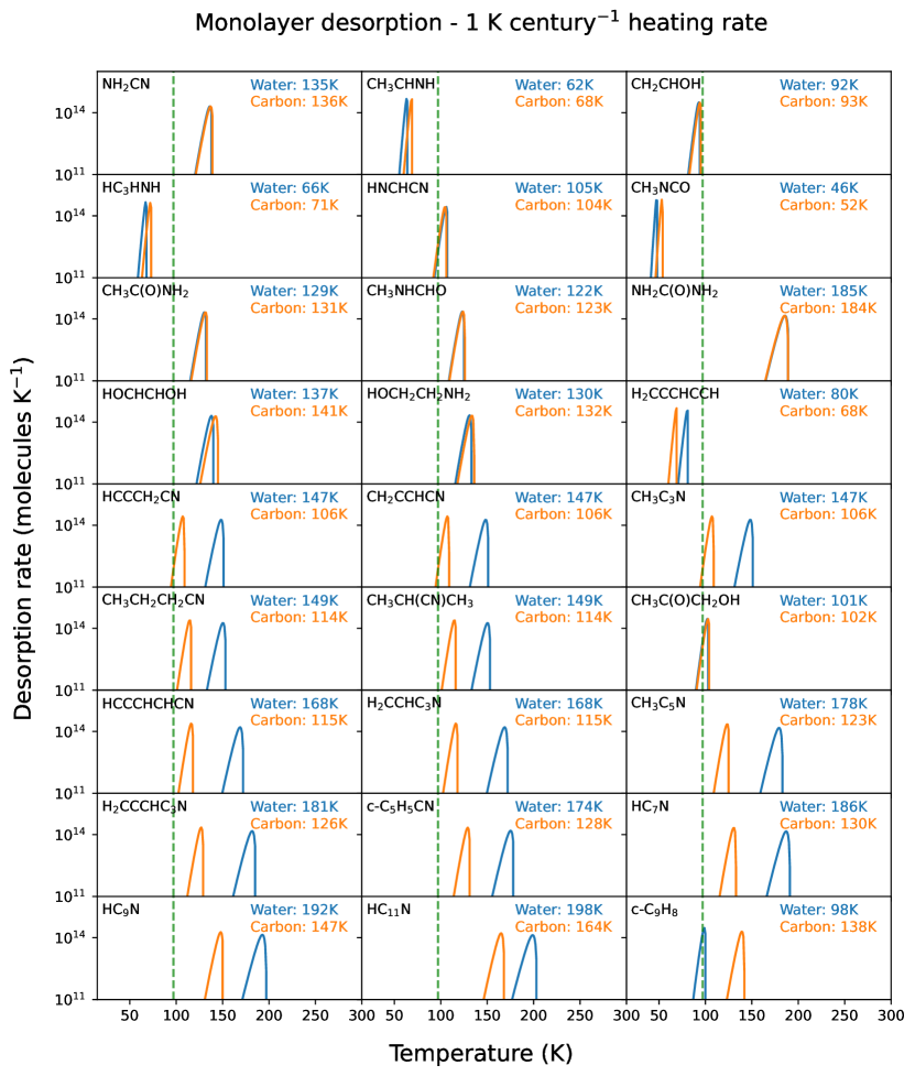
Figure 3: Desorption traces of molecules for which the BE is determined in this work. The first order desorption profiles are plotted for monolayer (1$\times$10¹⁵ molecules cm^-2) coverage on a water ice (blue) and carbonaceous (orange) surface. The peak desorption temperatures are indicated in the top right corners. A linear heating rate of 1 K century^-1 is applied. Prefactors are assumed and set at A = 1$\times$10¹⁸ s^-1 for all molecules. The peak desorption for water is indicated with a green dashed lines at 97 K.

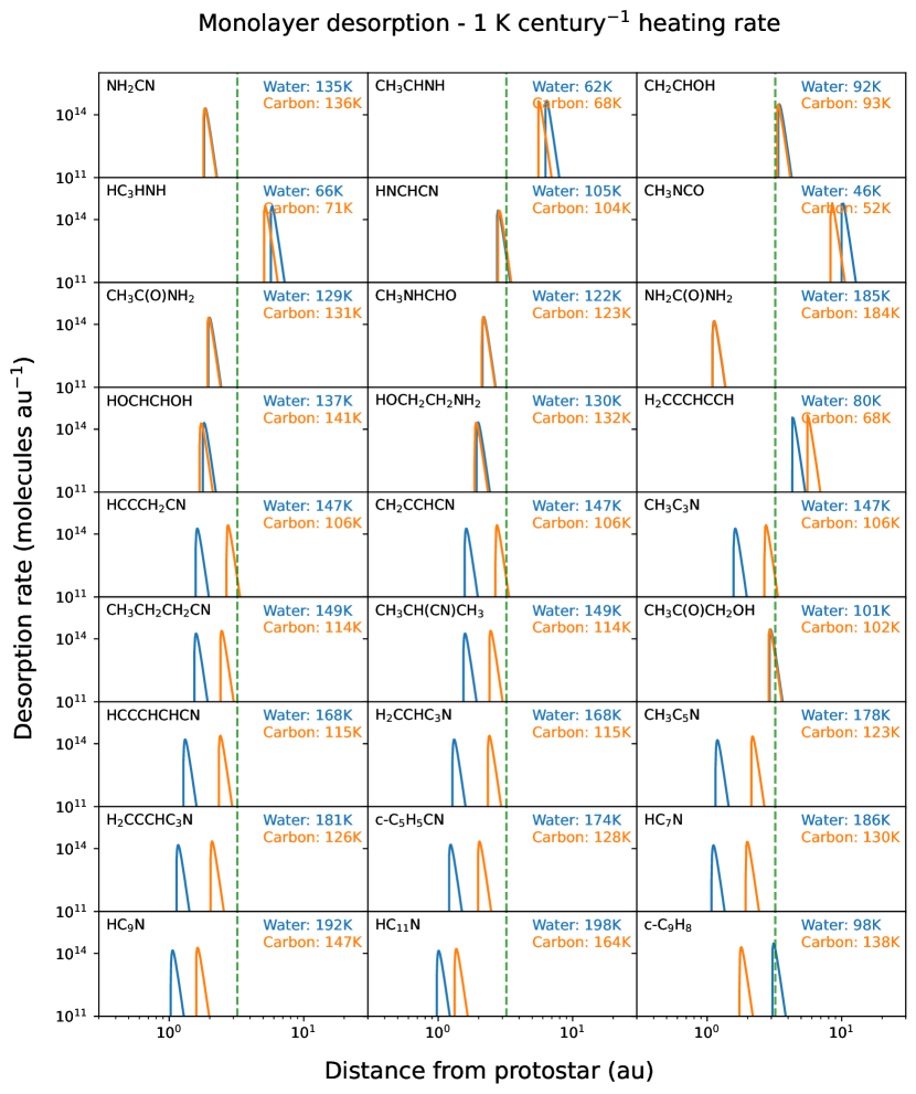
Figure 4: Same as Fig. 3, except that the desorption trace is plotted against a median disk temperature profile as derived by Andrews & Williams (2007), see main text for more details. Shorter distances are closer to the protostar and thus correspond to higher temperatures. The peak desorption for water is indicated with a green dashed lines at 3.2 au.

5 Conclusions

In this work, an ML model based on Gaussian Process Regression is created and trained to predict BEs of molecules, specifically those of astrochemical relevance. The BEs determined from laboratory experiments are collected, categorized by their features (e.g., mono- or multilayer coverage, binding surface, functional groups, valence electrons, H-bond acceptors and donors), and used as training data for the model. The performance of the model is assessed with five-fold and leave-one-molecule-out cross validation. A root mean square error of 892 K and 580 K are found, for the mono- and multilayer model, respectively. For individual molecules the deviation between model predicted and literature BEs is found to be within $\pm$20%. We note that sufficient training data and accurate feature representation are essential to predict BEs. Molecules for which features are not well described or insufficient training data points are available will generally have larger uncertainties on their predictions.

The validated model is used to predict the BEs on a water and carbonaceous surface of twenty one molecules that have been detected in recent years in the interstellar medium, but for which no or limited experimental information about their BEs is available. The lowest BE of 2990 K is predicted for methyl isocyanate (CH₃NCO) on a water surface, while the highest BE of 12820 K is predicted for cyanopentacetylene (HC₁₁N) bound to a water surface. Uncertainties on the predictions range from just a few percent to about 60% for hydroxyacetone (CH₃C(O)CH₂OH), which is presumably a reflection of the lack of training data and feature representation for these molecules. The surface can have a pronounced effect on the predicted BE, showing differences of several 1000’s K for some molecules. Finally, a comparison between the ML model predictions and the in the field of astrochemistry widely used linear addition method to predict BEs is presented. We find that the linear addition methods generally overpredicts BEs, in some case by more than a factor of two.

The newly predicted BEs are put into context of interstellar environments with a simple model that shows their desorption profile with respect to a 1 K century^-1 temperature ramp and a protoplanetary disk temperature profile. From this simple model, the locations of the snowlines of these molecules are determined. Most of them will roughly coincide with the water snowline, but those of cyanamide (NH₂CN), urea/carbamide (NH₂C(O)NH₂), and the cyanoacetylenes (HC_xN) are located at much higher temperatures or closer to the protostar.

This work demonstrates that ML can be employed to accurately and rapidly predict BEs of molecules. The approach taken here is based on experimental training data, but we note that ML models can also be trained on BEs obtained from quantum chemical calculations, as already pursued intensively in the heterogeneous catalysis community (e.g., Gu et al., 2020; Fung et al., 2021; Andersen & Reuter, 2021). In that connection, a natural extension of this work could be to also take into account BE distributions on amorphous and highly anisotropic surfaces, as this distribution is often readily available from quantum chemical calculations (e.g., Tinacci et al., 2022; Ferrero et al., 2020; Duflot et al., 2021). Overall, we believe that the work presented here could pave the way for a stronger collaboration between the communities working on quantum chemical calculations of BEs, laboratory experiments and ML, as the various approaches complement each other. The here predicted BEs will find general use in the modelling of astrochemical and planet-forming environments, while more detailed BE distributions would be critical to more specific modelling such as the reactivity of molecules at dust grains at low temperatures.

Table 4: Comparison between predicted and observed values of BE obtained from the literature measured in eV and rounded to nearest 0.01.

Name	Molecule	Surface or Coverage	Prediction	Observation	Deviation
			(eV)	(eV)
Acetone	$\mathrm{CH}_{3}\mathrm{C(O)CH}_{3}$	Water	$0.39\pm 0.04$	0.40 $\pm$ 0.02	$-3.6$ %
Acetonitrile	$\mathrm{CH}_{3}\mathrm{CN}$	Metal	$0.58\pm 0.08$	0.48 $\pm$ 0.03	$21$ %
Allyl alcohol	$\mathrm{C}_{3}\mathrm{H}_{5}\mathrm{OH}$	Metal	0.61 $\pm$ 0.15	0.52† iiiiiii	$18$ %
Ammonia	$\mathrm{NH}_{3}$	Carbon	$0.25\pm 0.15$	0.26 $\pm$ 0.02	$-4.0$ %
Methane	$\mathrm{CH}_{4}$	Carbon	0.16 $\pm$ 0.04	0.15 $\pm$ 0.01	$10$ %
Methyl formate	$\mathrm{CH}_{3}\mathrm{OCHO}$	Water	$0.46\pm 0.04$	0.39 $\pm$ 0.05	$19$ %
Nonacosane	$\mathrm{C}_{29}\mathrm{H}_{60}$	Carbon	$2.04\pm 0.02$	2.04 $\pm$ 0.00	$0.0$ %
Thymine	$\mathrm{C}_{5}\mathrm{H}_{6}\mathrm{N}_{2}\mathrm{O}_{2}$	Metal	$1.01\pm 0.22$	1.11 $\pm$ 0.02	$-9.6$ %
Acetonitrile	$\mathrm{CH}_{3}\mathrm{CN}$	Multilayer	$0.35\pm 0.04$	0.42 $\pm$ 0.04	$-16$ %
Ammonia	$\mathrm{NH}_{3}$	Multilayer	$0.26\pm 0.10$	0.26 $\pm$ 0.01	$9.9$ %
Methyl formate	$\mathrm{CH}_{3}\mathrm{OCHO}$	Multilayer	$0.43\pm 0.09$	0.35 $\pm$ 0.02	$10$ %

Appendix A Cross validation

Figure 5 schematically displays how the five-fold cross validation is set up. Figure 6 depicts the parity plot when only BEs up to 17000 K are included.

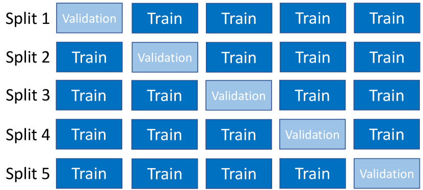
Figure 5: Schematic overview of 5-fold cross validation

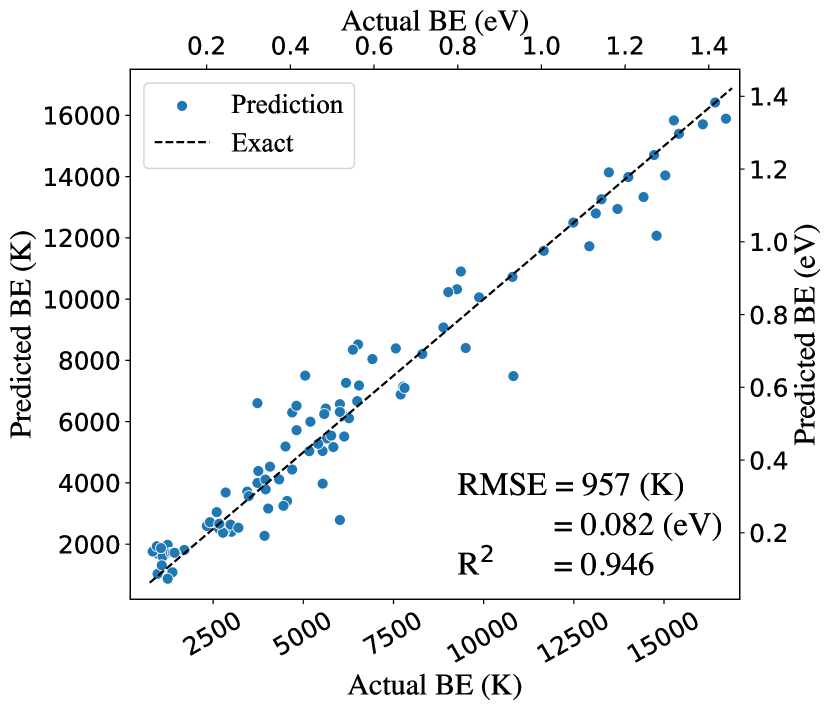
Figure 6: Parity plot for the monolayer case and including only BEs up to 17000 K.

Appendix B Literature data and molecular features

Table LABEL:tab:molecule_features shows the most important features of molecules that are used as training data in this work. Tables LABEL:tab:molecule_features and LABEL:tab:multilayer_data present the literature data used to train the ML model on.

Table 5: Features of molecules used for ML

Molecule	Molecule	Mass	atoms	-OH	-C(O)-	-COOH	-C(O)O-	-O-	-NH2	-CN	-N-C(O)-	Valence	H-bond	H-bond	TPSA
name	formula											electrons	acceptor	donor
		amu	#	#	#	#	#	#	#	#	#	#	#	#	Å2
Methane	CH4	16	5	–	–	–	–	–	–	–	–	8	0	0	0
Ammonia	NH3	17	4	–	–	–	–	–	–	–	–	8	1	1	35
Water	H2O	18	3	1	–	–	–	–	–	–	–	8	0	0	32
Acetylene	C2H2	26	4	–	–	–	–	–	–	–	–	10	0	0	0
Hydrogen cyanide	HCN	27	3	–	–	–	–	–	–	1	–	10	1	0	24
Carbon monoxide	CO	28	2	–	–	–	–	–	–	–	–	12	1	0	17
Ethylene	C2H4	28	6	–	–	–	–	–	–	–	–	12	0	0	0
Ethylene glycole	(CH2OH)2	62	10	2	–	–	–	–	–	–	–	12	2	2	40
Dinitrogen	N2	28	2	–	–	–	–	–	–	–	–	10	2	0	48
Ethane	C2H6	30	8	–	–	–	–	–	–	–	–	14	0	0	0
Formaldehyde	H2CO	30	4	–	1	–	–	–	–	–	–	12	1	0	17
Methylamine	CH3NH2	31	7	–	–	–	–	–	1	–	–	14	1	1	26
Methanol	CH3OH	32	6	1	–	–	–	–	–	–	–	14	1	1	20
Oxygen	O2	32	2	–	–	–	–	–	–	–	–	8	0	0	32
Hydroxylamine	NH2OH	33	5	1	–	–	–	–	1	–	–	14	2	2	46
Methylacetylene	CH3CCH	40	7	–	–	–	–	–	–	–	–	16	0	0	0
Acetonitrile	CH3CN	41	6	–	–	–	–	–	–	1	–	16	1	0	24
methylisocyanide	CH3NC	41	6	–	–	–	–	–	–	1	–	16	0	0	4
Propene	CH2CHCH3	42	9	–	–	–	–	–	–	–	–	18	0	0	0
Isocyanic acid	HNCO	43	4	–	–	–	–	–	–	–	–	16	2	1	41
Acetaldehyde	CH3CHO	44	7	–	1	–	–	–	–	–	–	18	1	0	17
Carbon dioxide	CO2	44	3	–	–	–	–	–	–	–	–	16	2	0	34
Ethylene oxide	c-C2H4O	44	7	–	–	–	–	1	–	–	–	18	1	0	13
Nitrous oxide	N2O	44	3	–	–	–	–	–	–	–	–	16	2	0	51
Propane	C3H8	44	11	–	–	–	–	–	–	–	–	20	0	0	0
Formamide	NH2CHO	45	6	–	–	–	–	–	–	–	1	18	1	1	43
Dimethylether	CH3OCH3	46	9	–	–	–	–	1	–	–	–	20	1	0	9
Ethanol	CH3CH2OH	46	9	1	–	–	–	–	–	–	–	20	1	1	20
Formic acid	HCOOH	46	5	–	–	1	–	–	–	–	–	18	1	1	37
Nitrogen dioxide	NO2	46	3	–	–	–	–	–	–	–	–	17	3	0	54
Cyanoacetylene	HC3N	51	5	–	–	–	–	–	–	1	–	18	1	0	24
Acrylonitrile	CH2CHCN	53	7	–	–	–	–	–	–	1	–	20	1	0	24
Propionitrile	CH3CH2CN	55	9	–	–	–	–	–	–	1	–	22	1	0	24
Acetone	CH3COCH3	58	10	–	1	–	–	–	–	–	–	24	1	0	17
Allyl alcohol	CH2CHCH2OH	58	10	1	–	–	–	–	–	–	–	24	1	1	20
Propionaldehyde	CH3CH2CHO	58	10	–	1	–	–	–	–	–	–	24	1	0	17
Acetic acid	CH3COOH	60	8	–	–	1	–	–	–	–	–	24	1	1	37
Glycolaldehyde	HOCH2CHO	60	8	1	1	–	–	–	–	–	–	24	2	1	37
Glycolonitrile	HOCH2CN	57	7	1	–	–	–	–	–	–	1	24	2	1	44
Methyl formate	CH3OCHO	60	8	–	–	–	1	–	–	–	–	24	2	0	26
Pentane	C5H12	72	17	–	–	–	–	–	–	–	–	32	0	0	0
N,N-DMF	(CH3)2NCHO	73	12	–	–	–	–	–	–	–	1	30	1	0	20
Ethyl formate	CH3CH2OCHO	74	11	–	–	–	1	–	–	–	–	30	2	0	26
Dicyanoacetylene	NCCCCN	76	6	–	–	–	–	–	–	2	–	26	2	0	48
Benzene	C6H6	78	12	–	–	–	–	–	–	–	–	30	0	0	0
Hexane	C6H14	86	20	–	–	–	–	–	–	–	–	38	0	0	0
Toluene	CH3C6H5	92	15	–	–	–	–	–	–	–	–	36	0	0	0
1,1-Dichloroethane	CH3CHCl2	98	8	–	–	–	–	–	–	–	–	26	0	0	0
Heptane	C7H16	100	23	–	–	–	–	–	–	–	–	44	0	0	0
Benzonitrile	c-C6H5CN	103	13	–	–	–	–	–	–	1	–	38	1	0	24
Benzaldehyde	C6H5CHO	106	14	–	1	–	–	–	–	–	–	40	1	0	17
Ethylbenzene	CH3CH2C6H5	106	18	–	–	–	–	–	–	–	–	42	0	0	0
o-Xylene	(CH3)2C6H4	106	18	–	–	–	–	–	–	–	–	42	0	0	0
Cytosine	C4H5N3O	111	13	–	–	–	–	–	1	–	1	42	3	2	72
Octane	C8H18	114	26	–	–	–	–	–	–	–	–	50	0	0	0
Trichloromethane	CHCl3	118	5	–	–	–	–	–	–	–	–	26	0	0	0
Thymine	C5H6N2O2	126	15	–	–	–	–	–	–	–	1	48	2	2	66
Naphthalene	C10H8	128	18	–	–	–	–	–	–	–	–	48	0	0	0
Nonane	C9H20	128	29	–	–	–	–	–	–	–	–	56	0	0	0
Adenine	C5H5N5	135	15	–	–	–	–	–	1	–	–	50	4	2	80
Decane	C10H22	142	32	–	–	–	–	–	–	–	–	62	0	0	0
1,2-Dichlorobenzene	C6H4Cl2	146	12	–	–	–	–	–	–	–	–	42	0	0	0
Guanine	C5H5N5O	151	16	–	–	–	–	–	1	–	1	56	4	3	100
Undecane	C11H24	156	35	–	–	–	–	–	–	–	–	68	0	0	0
Dodecane	C12H26	170	38	–	–	–	–	–	–	–	–	74	0	0	0
Tridecane	C13H28	184	41	–	–	–	–	–	–	–	–	80	0	0	0
Tetradecan	C14H30	198	44	–	–	–	–	–	–	–	–	86	0	0	0
Pentadecane	C15H32	212	47	–	–	–	–	–	–	–	–	92	0	0	0
Hexadecane	C16H34	226	50	–	–	–	–	–	–	–	–	98	0	0	0
Heptadecane	C17H36	240	53	–	–	–	–	–	–	–	–	104	0	0	0
2-Deoxyadenosine	C10H13N5O3	251	31	2	–	–	–	1	1	–	–	96	8	3	119
Octadecane	C18H38	254	56	–	–	–	–	–	–	–	–	110	0	0	0
2-Deoxyguanosine	C10H13N5O4	267	32	2	–	–	–	1	1	–	1	102	8	4	139
Nonadecane	C19H40	268	59	–	–	–	–	–	–	–	–	116	0	0	0
Icosane	C20H42	282	62	–	–	–	–	–	–	–	–	122	0	0	0
Henicosane	C21H44	296	65	–	–	–	–	–	–	–	–	128	0	0	0
Coronene	C24H12	300	36	–	–	–	–	–	–	–	–	108	0	0	0
Docosane	C22H46	310	68	–	–	–	–	–	–	–	–	134	0	0	0
Tricosane	C23H48	324	71	–	–	–	–	–	–	–	–	140	0	0	0
Coronene	C24H50	338	74	–	–	–	–	–	–	–	–	108	0	0	0
Tetracosane	C25H52	352	77	–	–	–	–	–	–	–	–	146	0	0	0
Pentacosane	C26H54	366	80	–	–	–	–	–	–	–	–	152	0	0	0
Hexacosane	C27H56	380	83	–	–	–	–	–	–	–	–	158	0	0	0
Heptacosane	C28H58	394	86	–	–	–	–	–	–	–	–	164	0	0	0
Octacosane	C29H60	408	89	–	–	–	–	–	–	–	–	170	0	0	0
Octacosane	C30H62	422	92	–	–	–	–	–	–	–	–	170	0	0	0
Nonacosane	C31H64	436	95	–	–	–	–	–	–	–	–	176	0	0	0
Dotriacontane	C32H66	450	98	–	–	–	–	–	–	–	–	194	0	0	0
Tritriacontane	C33H68	464	101	–	–	–	–	–	–	–	–	200	0	0	0
Tetratriacontane	C34H70	478	104	–	–	–	–	–	–	–	–	206	0	0	0
Pentatriacontane	C35H72	492	107	–	–	–	–	–	–	–	–	212	0	0	0
Hexatriacontane	C36H74	506	110	–	–	–	–	–	–	–	–	218	0	0	0
Heptatriacontane	C37H76	520	113	–	–	–	–	–	–	–	–	224	0	0	0
Octatriacontane	C38H78	534	116	–	–	–	–	–	–	–	–	230	0	0	0
Nonatriacontane	C39H80	548	119	–	–	–	–	–	–	–	–	236	0	0	0
Tetracontane	C40H82	562	122	–	–	–	–	–	–	–	–	242	0	0	0
Hentetracontane	C41H84	576	125	–	–	–	–	–	–	–	–	248	0	0	0
Dotetracontane	C42H86	590	128	–	–	–	–	–	–	–	–	254	0	0	0
Tritetracontane	C43H88	604	131	–	–	–	–	–	–	–	–	260	0	0	0
Tetratetracontane	C44H90	618	134	–	–	–	–	–	–	–	–	266	0	0	0
Pentatetracontane	C45H92	632	137	–	–	–	–	–	–	–	–	272	0	0	0
Hexatetracontane	C46H94	646	140	–	–	–	–	–	–	–	–	278	0	0	0
Heptatetracontane	C47H96	660	143	–	–	–	–	–	–	–	–	284	0	0	0
Octatetracontane	C48H98	674	146	–	–	–	–	–	–	–	–	290	0	0	0
Nonatetracontane	C49H100	688	149	–	–	–	–	–	–	–	–	296	0	0	0
Pentacontane	C50H102	702	152	–	–	–	–	–	–	–	–	302	0	0	0
Henpentacontane	C51H104	716	155	–	–	–	–	–	–	–	–	308	0	0	0
Dopentacontane	C52H106	730	158	–	–	–	–	–	–	–	–	314	0	0	0
Tripentacontane	C53H108	744	161	–	–	–	–	–	–	–	–	320	0	0	0
Tetrapentacontane	C54H110	758	164	–	–	–	–	–	–	–	–	326	0	0	0
Pentapentacontane	C55H112	772	167	–	–	–	–	–	–	–	–	332	0	0	0
Hexapentacontane	C56H114	786	170	–	–	–	–	–	–	–	–	338	0	0	0
Heptapentacontane	C57H116	800	173	–	–	–	–	–	–	–	–	344	0	0	0
Octapentacontane	C58H118	814	176	–	–	–	–	–	–	–	–	350	0	0	0
Nonapentacontane	C59H120	828	179	–	–	–	–	–	–	–	–	356	0	0	0
Hexacontane	C60H122	842	182	–	–	–	–	–	–	–	–	362	0	0	0

Table 6: BEs of molecules at monolayer coverage

Name	Formula	Surface	Simplified Surface	$E_{\rm bin}$	$E_{\rm bin}$	Reference
				(K)	(eV)
1,1-Dichloroethane	CH3CHCl2	HOPG	Carbon	16134 $\pm$ 0361	0.529 $\pm$ 0.031	Ulbricht et al. (2006)
1,2-Dichlorobenzene	C6H4Cl2	HOPG	Carbon	18299 $\pm$ 0722	0.715 $\pm$ 0.062	Ulbricht et al. (2006)
2-Deoxyadenosine	C10H13N5O3	Au(100)	Metal	13471 $\pm$ 0481	1.161 $\pm$ 0.041	Demers et al. (2002)
2-Deoxycytidine	C9H13N3O4	Au(100)	Metal	13711 $\pm$ 0241	1.182 $\pm$ 0.021	Demers et al. (2002)
2-Deoxyguanosine	C10H13N5O4	Au(100)	Metal	14433 $\pm$ 0241	1.244 $\pm$ 0.021	Demers et al. (2002)
Acetaldehyde	CH3CHO	Ni	Metal	12847 $\pm$ 0030	0.245 $\pm$ 0.003	Corazzi et al. (2021)
Acetaldehyde	CH3CHO	ASW	Water	14330 $\pm$ 0217	0.373 $\pm$ 0.019	Lasne et al. (2012)
Acetone	CH3COCH3	ASW	Water	14691 $\pm$ 0241	0.404 $\pm$ 0.021	Lasne et al. (2012)
Acetonitrile †	CH3CN	Ni	Metal	13305 $\pm$ 0013	0.285 $\pm$ 0.001	Corazzi et al. (2021)
Acetonitrile †	CH3CN	Olivine grains	Si	14400 $\pm$ 0200	0.379 $\pm$ 0.017	Corazzi et al. (2021)
Acetonitrile †	CH3CN	amorphous silica	Si	14595 $\pm$ 0120	0.396 $\pm$ 0.010	Abdulgalil et al. (2013)
Acetonitrile †	CH3CN	Pt(111)	Metal	14876 $\pm$ 0361	0.420 $\pm$ 0.031	Tylinski et al. (2020)
Acetonitrile †	CH3CN	alpha-quartz(0001)	Si	15225 $\pm$ 0696	0.450 $\pm$ 0.060	Bertin et al. (2017)
Acetonitrile †	CH3CN	Graphene	Carbon	15292 $\pm$ 0361	0.456 $\pm$ 0.031	Tylinski et al. (2020)
Acetonitrile †	CH3CN	Au(100)	Metal	15533 $\pm$ 0000	0.477 $\pm$ 0.000	Solomun et al. (1989)
Acetonitrile †	CH3CN	Graphene	Carbon	15653 $\pm$ 0361	0.487 $\pm$ 0.031	Tylinski et al. (2020)
Acetonitrile	CH3CN	ASW	Water	16184 $\pm$ 0406	0.533 $\pm$ 0.035	Bertin et al. (2017)
Acetylene	C2H2	compact ASW	Water	13200 $\pm$ 0220	0.276 $\pm$ 0.019	Behmard et al. (2019)
Acrylonitrile	CH2CHCN	Au	Metal	14215 $\pm$ 0051	0.363 $\pm$ 0.004	Toumi et al. (2016)
Adenine	C5H5N5	Au	Metal	14794 $\pm$ 0241	1.275 $\pm$ 0.021	Östblom et al. (2005)
Allyl alcohol	CH2CHCH2OH	Pd(111)	Metal	16014 $\pm$ 0000	0.518 $\pm$ 0.000	Dostert et al. (2016)
Ammonia †	NH3	HOPG	Carbon	12790 $\pm$ 0144	0.240 $\pm$ 0.012	Bolina et al. (2005b)
Ammonia †	NH3	Au	Metal	13007 $\pm$ 0120	0.259 $\pm$ 0.010	Noble et al. (2013)
Ammonia †	NH3	HOPG	Carbon	13007 $\pm$ 0241	0.259 $\pm$ 0.021	Ulbricht et al. (2006)
Ammonia †	NH3	Au	Metal	13067 $\pm$ 0012	0.264 $\pm$ 0.001	Kruczkiewicz et al. (2021)
Ammonia	NH3	Cut Forsterite (Mg2SiO4)	Si	13747 $\pm$ 0397	0.323 $\pm$ 0.034	Suhasaria et al. (2015)
Benzaldehyde	C6H5CHO	ASW	Water	14811 $\pm$ 0241	0.415 $\pm$ 0.021	Lasne et al. (2012)
Benzene	C6H6	ASW	Water	14691 $\pm$ 0000	0.404 $\pm$ 0.000	Bahr & Kempter (2007)
Benzene	C6H6	HOPG	Carbon	15623 $\pm$ 0962	0.485 $\pm$ 0.083	Ulbricht et al. (2006)
Benzonitrile	c-C6H5CN	Au(100)	Metal	19020 $\pm$ 0000	0.777 $\pm$ 0.000	Solomun et al. (1989)
C11H24	C11H24	Graphite	Carbon	13266 $\pm$ 0530	1.143 $\pm$ 0.046	a
C12H26	C12H26	Graphite	Carbon	14011 $\pm$ 0560	1.207 $\pm$ 0.048	a
C13H28	C13H28	Graphite	Carbon	14726 $\pm$ 0589	1.269 $\pm$ 0.051	a
C14H30	C14H30	Graphite	Carbon	15413 $\pm$ 0616	1.328 $\pm$ 0.053	a
C15H32	C15H32	Graphite	Carbon	16077 $\pm$ 0643	1.385 $\pm$ 0.055	a
C16H34	C16H34	Graphite	Carbon	16718 $\pm$ 0668	1.441 $\pm$ 0.058	a
C17H36	C17H36	Graphite	Carbon	17340 $\pm$ 0693	1.494 $\pm$ 0.060	a
C18H38	C18H38	Graphite	Carbon	17944 $\pm$ 0717	1.546 $\pm$ 0.062	a
C19H40	C19H40	Graphite	Carbon	18531 $\pm$ 0741	1.597 $\pm$ 0.064	a
C20H42	C20H42	Graphite	Carbon	19103 $\pm$ 0764	1.646 $\pm$ 0.066	a
C21H44	C21H44	Graphite	Carbon	19661 $\pm$ 0786	1.694 $\pm$ 0.068	a
C22H46	C22H46	Graphite	Carbon	20206 $\pm$ 0808	1.741 $\pm$ 0.070	a
C23H48	C23H48	Graphite	Carbon	20738 $\pm$ 0829	1.787 $\pm$ 0.071	a
C24H50	C24H50	Graphite	Carbon	21259 $\pm$ 0850	1.832 $\pm$ 0.073	a
C25H52	C25H52	Graphite	Carbon	21770 $\pm$ 0870	1.876 $\pm$ 0.075	a
C26H54	C26H54	Graphite	Carbon	22270 $\pm$ 0890	1.919 $\pm$ 0.077	a
C27H56	C27H56	Graphite	Carbon	22761 $\pm$ 0910	1.961 $\pm$ 0.078	a
C28H58	C28H58	Graphite	Carbon	23242 $\pm$ 0930	2.003 $\pm$ 0.080	a
C29H60	C29H60	Graphite	Carbon	23715 $\pm$ 0949	2.044 $\pm$ 0.082	a
C30H62	C30H62	Graphite	Carbon	24181 $\pm$ 0967	2.084 $\pm$ 0.083	a
C31H64	C31H64	Graphite	Carbon	24638 $\pm$ 0986	2.123 $\pm$ 0.085	a
C33H68	C33H68	Graphite	Carbon	25531 $\pm$ 1021	2.200 $\pm$ 0.088	a
C34H70	C34H70	Graphite	Carbon	25967 $\pm$ 1039	2.238 $\pm$ 0.090	a
C35H72	C35H72	Graphite	Carbon	26397 $\pm$ 1056	2.275 $\pm$ 0.091	a
C36H74	C36H74	Graphite	Carbon	26821 $\pm$ 1073	2.311 $\pm$ 0.092	a
C37H76	C37H76	Graphite	Carbon	27239 $\pm$ 1090	2.347 $\pm$ 0.094	a
C38H78	C38H78	Graphite	Carbon	27652 $\pm$ 1106	2.383 $\pm$ 0.095	a
C39H80	C39H80	Graphite	Carbon	28059 $\pm$ 1122	2.418 $\pm$ 0.097	a
C40H82	C40H82	Graphite	Carbon	28461 $\pm$ 1138	2.453 $\pm$ 0.098	a
C41H84	C41H84	Graphite	Carbon	28858 $\pm$ 1154	2.487 $\pm$ 0.099	a
C42H86	C42H86	Graphite	Carbon	29250 $\pm$ 1170	2.521 $\pm$ 0.101	a
C43H88	C43H88	Graphite	Carbon	29637 $\pm$ 1185	2.554 $\pm$ 0.102	a
C44H90	C44H90	Graphite	Carbon	30020 $\pm$ 1201	2.587 $\pm$ 0.103	a
C45H92	C45H92	Graphite	Carbon	30399 $\pm$ 1216	2.620 $\pm$ 0.105	a
C46H94	C46H94	Graphite	Carbon	30773 $\pm$ 1231	2.652 $\pm$ 0.106	a
C47H96	C47H96	Graphite	Carbon	31144 $\pm$ 1246	2.684 $\pm$ 0.107	a
C48H98	C48H98	Graphite	Carbon	31510 $\pm$ 1260	2.715 $\pm$ 0.109	a
C49H100	C49H100	Graphite	Carbon	31873 $\pm$ 1275	2.747 $\pm$ 0.110	a
C50H102	C50H102	Graphite	Carbon	32232 $\pm$ 1289	2.778 $\pm$ 0.111	a
C51H104	C51H104	Graphite	Carbon	32587 $\pm$ 1303	2.808 $\pm$ 0.112	a
C52H106	C52H106	Graphite	Carbon	32939 $\pm$ 1318	2.838 $\pm$ 0.114	a
C53H108	C53H108	Graphite	Carbon	33288 $\pm$ 1332	2.869 $\pm$ 0.115	a
C54H110	C54H110	Graphite	Carbon	33633 $\pm$ 1345	2.898 $\pm$ 0.116	a
C55H112	C55H112	Graphite	Carbon	33975 $\pm$ 1359	2.928 $\pm$ 0.117	a
C56H114	C56H114	Graphite	Carbon	34314 $\pm$ 1373	2.957 $\pm$ 0.118	a
C57H116	C57H116	Graphite	Carbon	34650 $\pm$ 1386	2.986 $\pm$ 0.119	a
C58H118	C58H118	Graphite	Carbon	34983 $\pm$ 1399	3.015 $\pm$ 0.121	a
C59H120	C59H120	Graphite	Carbon	35314 $\pm$ 1413	3.043 $\pm$ 0.122	a
C60H122	C60H122	Graphite	Carbon	35641 $\pm$ 1426	3.071 $\pm$ 0.123	a
C9H20	C9H20	Graphite	Carbon	11667 $\pm$ 0467	1.005 $\pm$ 0.040	a
Carbon dioxide †	CO2	ASW	Water	12105 $\pm$ 0902	0.181 $\pm$ 0.078	Edridge et al. (2013)
Carbon dioxide †	CO2	non-porous ASW	Water	12236 $\pm$ 0025	0.193 $\pm$ 0.002	Noble et al. (2012)
Carbon dioxide †	CO2	np-ASW	Water	12250 $\pm$ 0020	0.194 $\pm$ 0.002	He et al. (2017)
Carbon dioxide †	CO2	Amorphous silicate	Si	12271 $\pm$ 0025	0.196 $\pm$ 0.002	Noble et al. (2012)
Carbon dioxide †	CO2	crystalline H2O	Water	12361 $\pm$ 0025	0.203 $\pm$ 0.002	Noble et al. (2012)
Carbon dioxide †	CO2	crystalline H2O	Water	12393 $\pm$ 0241	0.206 $\pm$ 0.021	Galvez et al. (2007)
Carbon dioxide †	CO2	HOPG	Carbon	12430 $\pm$ 0277	0.209 $\pm$ 0.024	Edridge et al. (2013)
Carbon dioxide †	CO2	ASW	Water	12490 $\pm$ 0241	0.215 $\pm$ 0.021	Galvez et al. (2007)
Carbon dioxide †	CO2	Forsterite (Mg2SiO4)	Si	12514 $\pm$ 0036	0.217 $\pm$ 0.003	Suhasaria et al. (2017)
Carbon dioxide †	CO2	HAC1	Carbon	12706 $\pm$ 0024	0.233 $\pm$ 0.002	Maté et al. (2019)
Carbon dioxide †	CO2	HAC2	Carbon	12814 $\pm$ 0024	0.242 $\pm$ 0.002	Maté et al. (2019)
Carbon dioxide †	CO2	H2O	Water	12860 $\pm$ 0200	0.246 $\pm$ 0.017	Sandford & Allamandola (1990)
Carbon dioxide †	CO2	Graphene	Carbon	13019 $\pm$ 0180	0.260 $\pm$ 0.016	Takeuchi et al. (2017)
Carbon dioxide †	CO2	Graphene	Carbon	13139 $\pm$ 0241	0.270 $\pm$ 0.021	Smith & Kay (2019)
Carbon monoxide †	CO	Au	Metal	10826 $\pm$ 0024	0.071 $\pm$ 0.002	Collings et al. (2003)
Carbon monoxide †	CO	Au	Metal	10855 $\pm$ 0025	0.074 $\pm$ 0.002	Bisschop et al. (2006)
Carbon monoxide †	CO	Au	Metal	10855 $\pm$ 0025	0.074 $\pm$ 0.002	Öberg et al. (2005)
Carbon monoxide †	CO	Au (polycrystaline)	Metal	10855 $\pm$ 0024	0.074 $\pm$ 0.002	Fuchs et al. (2006)
Carbon monoxide †	CO	non-porous ASW	Water	10863 $\pm$ 0025	0.074 $\pm$ 0.002	Noble et al. (2012)
Carbon monoxide †	CO	Amorphous silicate	Si	10867 $\pm$ 0025	0.075 $\pm$ 0.000	Noble et al. (2012)
Carbon monoxide †	CO	non-porous ASW	Water	10870 $\pm$ 0000	0.075 $\pm$ 0.000	He et al. (2016)
Carbon monoxide †	CO	Amorphous silica	Si	10878 $\pm$ 0036	0.076 $\pm$ 0.003	Collings et al. (2015)
Carbon monoxide †	CO	Graphene	Carbon	10958 $\pm$ 0052	0.083 $\pm$ 0.004	Smith et al. (2016)
Carbon monoxide †	CO	porous ASW	Water	10980 $\pm$ 0000	0.084 $\pm$ 0.000	He et al. (2016)
Carbon monoxide †	CO	crystalline H2O	Water	11009 $\pm$ 0025	0.087 $\pm$ 0.002	Noble et al. (2012)
Carbon monoxide †	CO	ASW	Water	11016 $\pm$ 0036	0.088 $\pm$ 0.003	Allouche et al. (1998)
Carbon monoxide †	CO	Forsterite (Mg2SiO4)	Si	11119 $\pm$ 0012	0.096 $\pm$ 0.001	Suhasaria et al. (2017)
Carbon monoxide †	CO	Amorphous silica	Si	11143 $\pm$ 0157	0.098 $\pm$ 0.014	Collings et al. (2015)
Carbon monoxide †	CO	compact ASW	Water	11155 $\pm$ 0133	0.100 $\pm$ 0.011	Fayolle et al. (2016)
Carbon monoxide †	CO	high porous ASW	Water	11179 $\pm$ 0024	0.102 $\pm$ 0.002	Collings et al. (2003)
Carbon monoxide †	CO	compact ASW	Water	11180 $\pm$ 0131	0.102 $\pm$ 0.011	Fayolle et al. (2016)
Carbon monoxide †	CO	HAC1	Carbon	11239 $\pm$ 0024	0.107 $\pm$ 0.002	Maté et al. (2019)
Carbon monoxide †	CO	HAC2	Carbon	11275 $\pm$ 0024	0.110 $\pm$ 0.002	Maté et al. (2019)
Carbon monoxide †	CO	ASW	Water	11419 $\pm$ 0071	0.122 $\pm$ 0.006	Smith et al. (2016)
Carbon monoxide †	CO	HOPG	Carbon	11564 $\pm$ 0120	0.135 $\pm$ 0.010	Ulbricht et al. (2006)
Cytosine	C4H5N3O	Au(100)	Metal	15035 $\pm$ 0481	1.296 $\pm$ 0.041	Demers et al. (2002)
Decane	C10H22	MgO(100)	Metal	19369 $\pm$ 0000	0.807 $\pm$ 0.000	Tait et al. (2005)
Decane	C10H22	Graphite	Carbon	12486 $\pm$ 0499	1.076 $\pm$ 0.043	a
Dicyanoacetylene	NCCCCN	ASW	Water	15052 $\pm$ 0601	0.435 $\pm$ 0.052	Guennoun et al. (2005)
Dicyanoacetylene	NCCCCN	Au	Metal	16134 $\pm$ 0601	0.529 $\pm$ 0.052	Guennoun et al. (2005)
Dimethylether	CH3OCH3	Au (polycrystaline)	Metal	13300 $\pm$ 0400	0.284 $\pm$ 0.034	Öberg et al. (2009)
Dimethylether	CH3OCH3	Crystalline H2O	Water	14076 $\pm$ 0503	0.351 $\pm$ 0.043	Lattelais et al. (2011)
Dotriacontane	C32H66	Graphite	Carbon	25089 $\pm$ 1004	2.162 $\pm$ 0.086	a
Ethane	C2H6	Au	Metal	12300 $\pm$ 0300	0.198 $\pm$ 0.026	Öberg et al. (2009)
Ethane	C2H6	porous ASW	Water	12663 $\pm$ 0000	0.229 $\pm$ 0.000	Behmard et al. (2019)
Ethane	C2H6	MgO(100)	Metal	12670 $\pm$ 0000	0.230 $\pm$ 0.000	Tait et al. (2005)
Ethane	C2H6	Graphene	Carbon	12983 $\pm$ 0149	0.257 $\pm$ 0.013	Smith et al. (2016)
Ethanol	CH3CH2OH	HOPG	Carbon	16014 $\pm$ 0361	0.518 $\pm$ 0.031	Ulbricht et al. (2006)
Ethyl formate	CH3CH2OCHO	HOPG	Carbon	15196 $\pm$ 0361	0.448 $\pm$ 0.031	Salter et al. (2019)
Ethyl formate	CH3CH2OCHO	ASW	Water	15833 $\pm$ 0241	0.503 $\pm$ 0.021	Salter et al. (2019)
Ethylene	C2H4	porous ASW	Water	12600 $\pm$ 0000	0.224 $\pm$ 0.000	Behmard et al. (2019)
Formaldehyde	H2CO	Au	Metal	13765 $\pm$ 0060	0.324 $\pm$ 0.005	Noble et al. (2012)
Formamide	NH2CHO	Ru(001)	Metal	16545 $\pm$ 0000	0.564 $\pm$ 0.000	Parmeter et al. (1988)
Formamide	NH2CHO	np-ASW	Water	17700 $\pm$ 0000	0.664 $\pm$	Chaabouni et al. (2018)
Formamide	NH2CHO	HOPG	Carbon	17770 $\pm$ 0000	0.670 $\pm$ 0.000	Chaabouni et al. (2018)
Guanine	C5H5N5O	Au(100)	Metal	16418 $\pm$ 0241	1.415 $\pm$ 0.021	Demers et al. (2002)
Heptane	C7H16	Graphite	Carbon	19874 $\pm$ 0395	0.851 $\pm$ 0.034	a
Hexane	C6H14	MgO(100)	Metal	15581 $\pm$ 0000	0.481 $\pm$ 0.000	Tait et al. (2005)
Hexane	C6H14	Graphite	Carbon	18886 $\pm$ 0355	0.766 $\pm$ 0.031	a
Hydroxylamine	NH2OH	Amorphous silicate	Si	16519 $\pm$ 0024	0.562 $\pm$ 0.002	Congiu et al. (2012)
Isocyanic acid †	HNCO	HOPG	Carbon	13729 $\pm$ 0192	0.321 $\pm$ 0.017	Noble et al. (2015)
Isocyanic acid †	HNCO	HOPG	Carbon	13957 $\pm$ 0204	0.341 $\pm$ 0.018	Noble et al. (2015)
Isocyanic acid	HNCO	Copper	Metal	14450 $\pm$ 0000	0.383 $\pm$ 0.000	Theulé et al. (2011)
Methane	CH4	Forsterite (Mg2SiO4)	Si	11323 $\pm$ 0012	0.114 $\pm$ 0.001	Suhasaria et al. (2017)
Methane	CH4	ASW	Water	11371 $\pm$ 0069	0.118 $\pm$ 0.006	Smith et al. (2016)
Methane	CH4	MgO(100)	Metal	11455 $\pm$ 0000	0.125 $\pm$ 0.000	Tait et al. (2005)
Methane	CH4	HOPG	Carbon	11702 $\pm$ 0120	0.147 $\pm$ 0.010	Ulbricht et al. (2006)
Methanol	CH3OH	Au	Metal	14700 $\pm$ 0500	0.405 $\pm$ 0.043	Öberg et al. (2009)
Methanol	CH3OH	ASW	Water	15412 $\pm$ 0000	0.466 $\pm$ 0.000	Bahr et al. (2008)
Methanol	CH3OH	HOPG	Carbon	15773 $\pm$ 0361	0.497 $\pm$ 0.031	Ulbricht et al. (2006)
Methyl formate	CH3OCHO	Au	Metal	14000 $\pm$ 0400	0.345 $\pm$ 0.034	Öberg et al. (2009)
Methyl formate	CH3OCHO	HOPG	Carbon	14210 $\pm$ 0000	0.363 $\pm$ 0.000	Burke et al. (2015a)
Methyl formate	CH3OCHO	Crystalline H2O	Water	14506 $\pm$ 0529	0.388 $\pm$ 0.046	Burke et al. (2015b)
Methylacetylene	CH3CCH	porous ASW	Water	14550 $\pm$ 0230	0.392 $\pm$ 0.020	Behmard et al. (2019)
Methylamine	CH3NH2	np-ASW	Water	14200 $\pm$ 0000	0.362 $\pm$ 0.000	Chaabouni et al. (2018)
Methylamine	CH3NH2	HOPG	Carbon	17000 $\pm$ 0000	0.603 $\pm$ 0.000	Chaabouni et al. (2018)
Methylisocyanide	CH3NC	Au	Metal	14352 $\pm$ 0116	0.375 $\pm$ 0.010	Bertin et al. (2017)
Methylisocyanide	CH3NC	alpha-quartz(0001)	Si	15165 $\pm$ 0812	0.445 $\pm$ 0.070	Bertin et al. (2017)
Methylisocyanide	CH3NC	ASW	Water	16267 $\pm$ 0348	0.540 $\pm$ 0.030	Bertin et al. (2017)
N,N-Dimethylformamide	(CH3)2NCHO	HOPG	Carbon	16374 $\pm$ 0481	0.549 $\pm$ 0.041	Ulbricht et al. (2006)
Naphthalene	C10H8	HOPG	Carbon	19261 $\pm$ 1082	0.798 $\pm$ 0.093	Ulbricht et al. (2006)
Nitrogen †	N2	Graphene	Carbon	10782 $\pm$ 0039	0.067 $\pm$ 0.003	Smith et al. (2016)
Nitrogen †	N2	Au	Metal	10790 $\pm$ 0025	0.068 $\pm$ 0.002	Öberg et al. (2005)
Nitrogen †	N2	Au (polycrystaline)	Metal	10790 $\pm$ 0025	0.068 $\pm$	Fuchs et al. (2006)
Nitrogen †	N2	non-porous ASW	Water	10790 $\pm$ 0000	0.068 $\pm$ 0.000	He et al. (2016)
Nitrogen †	N2	Au (polycrystaline)	Metal	10800 $\pm$ 0025	0.069 $\pm$ 0.002	Bisschop et al. (2006)
Nitrogen †	N2	porous ASW	Water	10900 $\pm$ 0000	0.078 $\pm$ 0.000	He et al. (2016)
Nitrogen †	N2	compact ASW	Water	11034 $\pm$ 0133	0.089 $\pm$ 0.011	Fayolle et al. (2016)
Nitrogen †	N2	nonporous ASW	Water	11082 $\pm$ 0120	0.093 $\pm$ 0.010	Zubkov et al. (2007)
Nitrogen †	N2	HAC1	Carbon	11119 $\pm$ 0024	0.096 $\pm$ 0.002	Maté et al. (2019)
Nitrogen †	N2	ASW	Water	11155 $\pm$ 0058	0.100 $\pm$ 0.005	Smith et al. (2016)
Nitrogen	N2	Amorphous silica	Si	11203 $\pm$ 0145	0.104 $\pm$ 0.012	Collings et al. (2015)
Nitrogen †	N2	HAC2	Carbon	11203 $\pm$ 0024	0.104 $\pm$ 0.002	Maté et al. (2019)
Nitrogen †	N2	Graphene	Carbon	11395 $\pm$ 0070	0.120 $\pm$ 0.006	Smith et al. (2016)
Nitrogen dioxide	NO2	HOPG	Carbon	14450 $\pm$ 0722	0.383 $\pm$ 0.062	Ulbricht et al. (2006)
Nitrous oxide	N2O	Amorphous silicate	Si	12772 $\pm$ 0018	0.239 $\pm$ 0.002	Congiu et al. (2012)
Octane	C8H18	MgO(100)	Metal	17565 $\pm$ 0000	0.652 $\pm$ 0.000	Tait et al. (2005)
Octane	C8H18	Graphite	Carbon	10800 $\pm$ 0432	0.931 $\pm$ 0.037	a
Oxygen †	O2	non-porous ASW	Water	10914 $\pm$ 0025	0.079 $\pm$ 0.002	Noble et al. (2012)
Oxygen †	O2	non-porous ASW	Water	10920 $\pm$ 0000	0.079 $\pm$ 0.000	He et al. (2016)
Oxygen	O2	Au (polycrystaline)	Metal	10925 $\pm$ 0025	0.080 $\pm$ 0.002	Fuchs et al. (2006)
Oxygen †	O2	Amorphous silicate	Si	10930 $\pm$ 0025	0.080 $\pm$ 0.002	Noble et al. (2012)
Oxygen †	O2	crystalline H2O	Water	10969 $\pm$ 0025	0.084 $\pm$ 0.002	Noble et al. (2012)
Oxygen †	O2	ASW	Water	11107 $\pm$ 0055	0.095 $\pm$ 0.005	Smith et al. (2016)
Oxygen †	O2	Amorphous silica	Si	11178 $\pm$ 0218	0.102 $\pm$ 0.019	Collings et al. (2015)
Oxygen †	O2	Forsterite (Mg2SiO4)	Si	11179 $\pm$ 0012	0.102 $\pm$ 0.001	Suhasaria et al. (2017)
Oxygen †	O2	Graphene	Carbon	11419 $\pm$ 0071	0.122 $\pm$ 0.006	Smith et al. (2016)
Oxygen †	O2	HOPG	Carbon	11443 $\pm$ 0120	0.124 $\pm$ 0.010	Ulbricht et al. (2006)
Pentane	C5H12	Graphite	Carbon	17808 $\pm$ 0312	0.673 $\pm$ 0.027	a
Propane	C3H8	compact ASW	Water	13446 $\pm$ 0280	0.297 $\pm$ 0.024	Behmard et al. (2019)
Propane	C3H8	MgO(100)	Metal	13488 $\pm$ 0000	0.301 $\pm$ 0.000	Tait et al. (2005)
Propane	C3H8	Graphene	Carbon	13752 $\pm$ 0188	0.323 $\pm$ 0.016	Smith et al. (2016)
Propene	CH2CHCH3	porous ASW	Water	13950 $\pm$ 0060	0.340 $\pm$ 0.005	Behmard et al. (2019)
Thymine	C5H6N2O2	Au(100)	Metal	12930 $\pm$ 0241	1.114 $\pm$ 0.021	Demers et al. (2002)
Toluene	CH3C6H5	HOPG	Carbon	16916 $\pm$ 0842	0.596 $\pm$ 0.073	Ulbricht et al. (2006)
Trichloromethane	CHCl3	HOPG	Carbon	16495 $\pm$ 0361	0.560 $\pm$ 0.031	Ulbricht et al. (2006)
Water †	H2O	Amorphous silica	Si	14210 $\pm$ 0120	0.363 $\pm$ 0.010	Collings et al. (2015)
Water †	H2O	Forsterite (Mg2SiO4(011))	Si	16014 $\pm$ 0000	0.518 $\pm$ 0.000	Smith et al. (2014)

Table 7: BEs of molecules at multilayer coverage

Name	Formula	Surface	$E_{\rm bin}$	$E_{\rm bin}$	Reference
			(K)	(eV)
1,1-Dichloroethane	CH3CHCl2	HOPG	5292 $\pm$ 361	0.456 $\pm$ 0.031	Ulbricht et al. (2006)
1,2-Dichlorobenzene	C6H4Cl2	HOPG	16735 $\pm$ 0601	0.580 $\pm$ 0.052	Ulbricht et al. (2006)
Acetic acid	CH3COOH	Au	5730 $\pm$ 024	0.494 $\pm$ 0.002	Kruczkiewicz et al. (2021)
Acetonitrile †	CH3CN	amorphous silica	4595 $\pm$ 120	0.396 $\pm$ 0.010	Abdulgalil et al. (2013)
Acetonitrile †	CH3CN	Pt(111)	4876 $\pm$ 361	0.420 $\pm$ 0.031	Tylinski et al. (2020)
Acetonitrile †	CH3CN	Graphene	5292 $\pm$ 361	0.456 $\pm$ 0.031	Tylinski et al. (2020)
Acetylene	C2H2	CsI	2800 $\pm$ 300	0.241 $\pm$ 0.026	Behmard et al. (2019)
Acrylonitrile	CH2CHCN	Au	4215 $\pm$ 051	0.363 $\pm$ 0.004	Toumi et al. (2016)
Allyl alcohol	CH2CHCH2OH	Pd(111)	5292 $\pm$ 000	0.456 $\pm$ 0.000	Dostert et al. (2016)
Ammonia †	NH3	HOPG	2790 $\pm$ 144	0.240 $\pm$ 0.012	Bolina et al. (2005b)
Ammonia †	NH3	Au	3007 $\pm$ 120	0.259 $\pm$ 0.010	Noble et al. (2013)
Ammonia †	NH3	HOPG	3007 $\pm$ 241	0.259 $\pm$ 0.021	Ulbricht et al. (2006)
Ammonia †	NH3	Au	3067 $\pm$ 012	0.264 $\pm$ 0.001	Kruczkiewicz et al. (2021)
Ammonia †	NH3	Cleaved Forsterite (Mg2SiO4)	3103 $\pm$ 108	0.267 $\pm$ 0.009	Suhasaria et al. (2015)
Ammonia †	NH3	Cut Forsterite (Mg2SiO4)	3103 $\pm$ 084	0.267 $\pm$ 0.007	Suhasaria et al. (2015)
Ammonia †	NH3	Au	3127 $\pm$ 120	0.269 $\pm$ 0.010	Noble et al. (2013)
Benzene †	C6H6	ASW	5052 $\pm$ 000	0.435 $\pm$ 0.000	Bahr & Kempter (2007)
Benzene †	C6H6	HOPG	5383 $\pm$ 217	0.464 $\pm$ 0.019	Salter et al. (2018)
Carbon dioxide †	CO2	ASW	2019 $\pm$ 168	0.174 $\pm$ 0.014	Edridge et al. (2013)
Carbon dioxide †	CO2	Amorphous silicate	2269 $\pm$ 080	0.196 $\pm$ 0.007	Noble et al. (2012)
Carbon dioxide †	CO2	Forsterite (Mg2SiO4)	2574 $\pm$ 024	0.222 $\pm$ 0.002	Suhasaria et al. (2017)
Carbon dioxide †	CO2	Graphene	2877 $\pm$ 241	0.248 $\pm$ 0.021	Smith & Kay (2019)
Carbon dioxide †	CO2	H2O:CH3OH	2923 $\pm$ 289	0.252 $\pm$ 0.025	Edridge et al. (2013)
Carbon monoxide †	CO	Forsterite (Mg2SiO4)	0806 $\pm$ 024	0.069 $\pm$ 0.002	Suhasaria et al. (2017)
Carbon monoxide †	CO	Amorphous silicate	0831 $\pm$ 040	0.072 $\pm$ 0.003	Noble et al. (2012)
Carbon monoxide †	CO	crystalline H2O	0849 $\pm$ 055	0.073 $\pm$ 0.005	Noble et al. (2012)
Carbon monoxide †	CO	Au	0855 $\pm$ 025	0.074 $\pm$ 0.002	Bisschop et al. (2006)
Carbon monoxide †	CO	Au	0855 $\pm$ 025	0.074 $\pm$ 0.002	Öberg et al. (2005)
Carbon monoxide †	CO	Au (polycrystaline)	0855 $\pm$ 024	0.074 $\pm$ 0.002	Fuchs et al. (2006)
Carbon monoxide †	CO	O2	0856 $\pm$ 015	0.074 $\pm$ 0.001	Acharyya et al. (2007)
Carbon monoxide †	CO	Au	0858 $\pm$ 015	0.074 $\pm$ 0.001	Acharyya et al. (2007)
Carbon monoxide †	CO	Au	0858 $\pm$ 015	0.074 $\pm$ 0.001	Acharyya et al. (2007)
Carbon monoxide †	CO	CsI	0866 $\pm$ 068	0.075 $\pm$ 0.006	Fayolle et al. (2016)
Carbon monoxide †	CO	Amorphous silica	0878 $\pm$ 036	0.076 $\pm$ 0.003	Collings et al. (2015)
Carbon monoxide †	CO	Graphene	0958 $\pm$ 052	0.083 $\pm$ 0.004	Smith et al. (2016)
Carbon monoxide †	CO	ASW	1016 $\pm$ 036	0.088 $\pm$ 0.003	Allouche et al. (1998)
Carbon monoxide †	CO	CO	1280 $\pm$ 000	0.110 $\pm$ 0.000	Sandford & Allamandola (1988)
Cyanoacetylene †	HC3N	ASW	4691 $\pm$ 962	0.404 $\pm$ 0.083	Borget et al. (2001)
Cyanoacetylene †	HC3N	crystalline H2O	4691 $\pm$ 962	0.404 $\pm$ 0.083	Borget et al. (2001)
Dimethylether	CH3OCH3	Au (polycrystaline)	3300 $\pm$ 400	0.284 $\pm$ 0.034	Öberg et al. (2009)
Ethane †	C2H6	Au	2300 $\pm$ 300	0.198 $\pm$ 0.026	Öberg et al. (2009)
Ethane †	C2H6	Graphene	2558 $\pm$ 126	0.220 $\pm$ 0.011	Smith et al. (2016)
Ethane †	C2H6	CsI	2600 $\pm$ 300	0.224 $\pm$ 0.026	Behmard et al. (2019)
Ethanol	CH3CH2OH	HOPG	5367 $\pm$ 361	0.462 $\pm$ 0.031	Ulbricht et al. (2006)
Ethyl formate	CH3CH2OCHO	HOPG	5479 $\pm$ 084	0.472 $\pm$ 0.007	Salter et al. (2019)
Ethylbenzene	CH3CH2C6H5	HOPG	00 7818 $\pm$ 1203 0	0.674 $\pm$ 0.104	Ulbricht et al. (2006)
Ethylene	C2H4	CsI	2200 $\pm$ 000	0.190 $\pm$ 0.000	Behmard et al. (2019)
Ethylene glycole	(CH2OH)2	Au	7500 $\pm$ 800	0.646 $\pm$ 0.069	Öberg et al. (2009)
Ethylene oxide	c-C2H4O	Au	2405 $\pm$ 241	0.207 $\pm$ 0.021	Schriver et al. (2004)
Formaldehyde	H2CO	Au	3765 $\pm$ 060	0.324 $\pm$ 0.005	Noble et al. (2012)
Formamide	NH2CHO	np-ASW	17700 $\pm$ 0000	0.664 $\pm$	Chaabouni et al. (2018)
Formic acid †	HCOOH	Au	4607 $\pm$ 012	0.397 $\pm$ 0.001	Kruczkiewicz et al. (2021)
Formic acid †	HCOOH	Au	5000 $\pm$ 500	0.431 $\pm$ 0.043	Öberg et al. (2009)
Glycolaldehyde †	HOCH2CHO	HOPG	5629 $\pm$ 000	0.485 $\pm$ 0.000	Burke et al. (2015a)
Glycolaldehyde †	HOCH2CHO	Au	5900 $\pm$ 600	0.508 $\pm$ 0.052	Öberg et al. (2009)
Glycolonitrile	HOCH2CN	Au	6976 $\pm$ 000	0.601 $\pm$ 0.000	Danger et al. (2012)
Hydrogen cyanide †	HCN	Au	3368 $\pm$ 120	0.290 $\pm$ 0.010	Noble et al. (2013)
Hydrogen cyanide †	HCN	Au	3608 $\pm$ 120	0.311 $\pm$ 0.010	Noble et al. (2013)
Isocyanic acid	HNCO	Copper	4450 $\pm$ 000	0.383 $\pm$ 0.000	Theulé et al. (2011)
Methane †	CH4	HOPG	1266 $\pm$ 120	0.109 $\pm$ 0.010	Ulbricht et al. (2006)
Methane †	CH4	Forsterite (Mg2SiO4)	1371 $\pm$ 036	0.118 $\pm$ 0.003	Suhasaria et al. (2017)
Methanol †	CH3OH	Au	4700 $\pm$ 500	0.405 $\pm$ 0.043	Öberg et al. (2009)
Methanol †	CH3OH	HOPG	5533 $\pm$ 361	0.477 $\pm$ 0.031	Ulbricht et al. (2006)
Methyl formate †	CH3OCHO	Au	4000 $\pm$ 400	0.345 $\pm$ 0.034	Öberg et al. (2009)
Methyl formate †	CH3OCHO	HOPG	4210 $\pm$ 000	0.363 $\pm$ 0.000	Burke et al. (2015a)
Methylacetylene	CH3CCH	CsI	4200 $\pm$ 300	0.362 $\pm$ 0.026	Behmard et al. (2019)
Methylamine	CH3NH2	HOPG	3200 $\pm$ 000	0.276 $\pm$ 0.000	Chaabouni et al. (2018)
methylisocyanide	CH3NC	Au	4352 $\pm$ 116	0.375 $\pm$ 0.010	Bertin et al. (2017)
N,N-Dimethylformamide	(CH3)2NCHO	HOPG	5533 $\pm$ 481	0.477 $\pm$ 0.041	Ulbricht et al. (2006)
Naphthalene	C10H8	HOPG	19261 $\pm$ 1082	0.798 $\pm$ 0.093	Ulbricht et al. (2006)
Nitrogen †	N2	CsI	0770 $\pm$ 068	0.066 $\pm$ 0.006	Fayolle et al. (2016)
Nitrogen †	N2	Graphene	0782 $\pm$ 039	0.067 $\pm$ 0.003	Smith et al. (2016)
Nitrogen †	N2	Au	0790 $\pm$ 025	0.068 $\pm$ 0.002	Öberg et al. (2005)
Nitrogen †	N2	Au (polycrystaline)	0790 $\pm$ 025	0.068 $\pm$ 0.002	Fuchs et al. (2006)
Nitrogen †	N2	Au (polycrystaline)	0800 $\pm$ 025	0.069 $\pm$ 0.002	Bisschop et al. (2006)
Nitrogen †	N2	Amorphous silica	0830 $\pm$ 036	0.072 $\pm$ 0.003	Collings et al. (2015)
Nitrogen †	N2	Graphene	0866 $\pm$ 043	0.075 $\pm$ 0.004	Smith et al. (2016)
Nitrogen †	N2	Graphene	0866 $\pm$ 043	0.075 $\pm$ 0.004	Smith et al. (2016)
Nitrogen dioxide	NO2	HOPG	3969 $\pm$ 601	0.342 $\pm$ 0.052	Ulbricht et al. (2006)
o-Xylene	(CH3)2C6H4	HOPG	6832 $\pm$ 000	0.609 $\pm$ 0.000	Salter et al. (2018)
Oxygen †	O2	Amorphous silicate	0895 $\pm$ 036	0.077 $\pm$ 0.003	Noble et al. (2012)
Oxygen †	O2	non-porous ASW	0898 $\pm$ 030	0.077 $\pm$ 0.003	Noble et al. (2012)
Oxygen †	O2	Amorphous silica	0902 $\pm$ 024	0.078 $\pm$ 0.002	Collings et al. (2015)
Oxygen †	O2	Au (polycrystaline)	0925 $\pm$ 025	0.080 $\pm$ 0.002	Fuchs et al. (2006)
Oxygen †	O2	crystalline H2O	0936 $\pm$ 040	0.081 $\pm$ 0.003	Noble et al. (2012)
Oxygen †	O2	Forsterite (Mg2SiO4)	0998 $\pm$ 024	0.086 $\pm$ 0.002	Suhasaria et al. (2017)
Oxygen †	O2	Graphene	1034 $\pm$ 052	0.089 $\pm$ 0.004	Smith et al. (2016)
Oxygen †	O2	HOPG	1082 $\pm$ 120	0.093 $\pm$ 0.010	Ulbricht et al. (2006)
Oxygen †	O2	Graphene	1119 $\pm$ 056	0.096 $\pm$ 0.005	Smith et al. (2016)
Propane †	C3H8	Graphene	3187 $\pm$ 171	0.275 $\pm$ 0.015	Smith et al. (2016)
Propane †	C3H8	CsI	3600 $\pm$ 300	0.310 $\pm$ 0.026	Behmard et al. (2019)
Propene	CH2CHCH3	CsI	3500 $\pm$ 300	0.302 $\pm$ 0.026	Behmard et al. (2019)
Propionaldehyde	CH3CH2CHO	Pd(111)	4330 $\pm$ 000	0.373 $\pm$ 0.000	Dostert et al. (2016)
Propionitrile	CH3CH2CN	Au	4546 $\pm$ 084	0.392 $\pm$ 0.007	Couturier-Tamburelli et al. (2018)
Toluene	CH3C6H5	HOPG	6074 $\pm$ 722	0.523 $\pm$ 0.062	Ulbricht et al. (2006)
Trichloromethane	CHCl3	HOPG	5653 $\pm$ 361	0.487 $\pm$ 0.031	Ulbricht et al. (2006)
Water †	H2O	HOPG	4799 $\pm$ 096	0.414 $\pm$ 0.008	Bolina et al. (2005a); Brown & Bolina (2007)
Water †	H2O	HOPG	5533 $\pm$ 361	0.477 $\pm$ 0.031	Ulbricht et al. (2006)
Water †	H2O	Au	5773 $\pm$ 060	0.497 $\pm$ 0.005	Fraser et al. (2001)
Water †	H2O	Amorphous silica	5930 $\pm$ 240	0.511 $\pm$ 0.021	Collings et al. (2015)
Water †	H2O	Al2O3(1120)	5992 $\pm$ 101	0.516 $\pm$ 0.009	Haynes et al. (1992)

Appendix C Astrochemically relevant species

Table LABEL:tab:astro_species_features presents the features of the astrochemically relevant molecules for which BEs are predicted in this work.

Table 8: Features of astrochemically relevant molecules used for ML

Molecule	Molecule	Mass	-OH	-C(O)-	-COOH	-C(O)O-	-O-	-NH2	-CN	-N-C(O)-	Valence	H-bond	H-bond	TPSA
name	formula										electrons	acceptor	donor
		amu	#	#	#	#	#	#	#	#	#	#	#	Å2
Cyanamide	NH2CN	42	–	–	–	–	–	1	1	–	16	2	1	50
Ethanimine	CH3CHNH	43	–	–	–	–	–	–	–	–	20	1	1	26
Vinylalcohol	CH2CHOH	44	1	–	–	–	–	–	–	–	18	1	1	20
Propargylimine	HC3HNH	53	–	–	–	–	–	–	–	–	20	1	1	24
Cyanomethanimine	HNCHCN	54	–	–	–	–	–	–	1	–	20	2	1	48
Methyl isocyanate	CH3NCO	57	–	–	–	–	–	–	–	–	22	2	0	29
Acetamide	CH3C(O)NH2	59	–	–	–	–	–	–	–	1	24	1	1	43
N-Methylformamide	CH3NHCHO	59	–	–	–	–	–	–	–	1	24	1	1	29
Carbamide / Urea	NH2C(O)NH2	60	–	–	–	–	–	–	–	2	24	1	2	69
Ethenediol	HOCHCHOH	60	2	–	–	–	–	–	–	–	24	2	2	40
Ethanolamine	HOCH2CH2NH2	61	1	–	–	–	–	1	–	–	26	2	2	46
Allenyl acetylene	H2CCCHCCH	64	–	–	–	–	–	–	–	–	24	0	0	0
Propargyl cyanide	HCCCH2CN	65	–	–	–	–	–	–	1	–	24	1	0	24
Cyanoallene	CH2CCHCN	65	–	–	–	–	–	–	1	–	24	1	0	24
Cyanopropyne	CH3C3N	65	–	–	–	–	–	–	1	–	24	1	0	24
n-Propylcyanide	CH3CH2CH2CN	69	–	–	–	–	–	–	1	–	28	1	0	24
i-Propylcyanide	CH3CH(CN)CH3	69	–	–	–	–	–	–	1	–	28	1	0	24
Hydroxyacetone	CH3C(O)CH2OH	74	1	1	–	–	–	–	–	–	30	2	1	37
Cyanovinylacetylene	HCCCHCHCN	77	–	–	–	–	–	–	1	–	28	1	0	24
Vinylcyanoacetylene	H2CCHC3N	77	–	–	–	–	–	–	1	–	28	1	0	24
Methylcyanodiacetylene	CH3C5N	89	–	–	–	–	–	–	1	–	28	1	0	24
Cyanoacetyleneallene	H2CCCHC3N	89	–	–	–	–	–	–	1	–	36	1	0	24
1-cyano-1,3-cyclopentadiene	c-C5H5CN	91	–	–	–	–	–	–	1	–	34	1	0	20
Cyanotriacetylene	HC7N	99	–	–	–	–	–	–	1	–	34	1	0	24
Indene	c-C9H8	116	–	–	–	–	–	–	–	–	44	0	0	0
Cyanotetraacetylene	HC9N	123	–	–	–	–	–	–	1	–	42	1	0	24
Cyanopentaacetylene	HC11N	147	–	–	–	–	–	–	1	–	50	1	0	24

References

- Abdulgalil et al. (2013) Abdulgalil, A. G. M., Marchione, D., Thrower, J., et al. 2013, Philosophical Transactions of the Royal Society A: Mathematical, Physical and Engineering Sciences, 371, 20110586
- Acharyya et al. (2007) Acharyya, K., Fuchs, G., Fraser, H., Van Dishoeck, E., & Linnartz, H. 2007, Astronomy & Astrophysics, 466, 1005
- Aigrain et al. (2012) Aigrain, S., Pont, F., & Zucker, S. 2012, Monthly notices of the royal astronomical society, 419, 3147
- Allouche et al. (1998) Allouche, A., Verlaque, P., & Pourcin, J. 1998, The Journal of Physical Chemistry B, 102, 89
- Andersen & Reuter (2021) Andersen, M. & Reuter, K. 2021, Acc. Chem. Res., 54, 2741
- Andrews & Williams (2007) Andrews, S. M. & Williams, J. P. 2007, The Astrophysical Journal, 659, 705
- Bahr & Kempter (2007) Bahr, S. & Kempter, V. 2007, The Journal of chemical physics, 127, 074707
- Bahr et al. (2008) Bahr, S., Toubin, C., & Kempter, V. 2008, The Journal of chemical physics, 128, 134712
- Balbisi et al. (2022) Balbisi, M., Horvath, R. A., Szőri, M., & Jedlovszky, P. 2022, The Journal of Chemical Physics, 156, 184703
- Behmard et al. (2019) Behmard, A., Fayolle, E. C., Graninger, D. M., et al. 2019, The Astrophysical Journal, 875, 73
- Bellman (1966) Bellman, R. 1966, Science, 153, 34
- Belloche et al. (2019) Belloche, A., Garrod, R., Müller, H., et al. 2019, Astronomy & Astrophysics, 628, A10
- Bertin et al. (2017) Bertin, M., Doronin, M., Fillion, J.-H., et al. 2017, Astronomy & Astrophysics, 598, A18
- Bisschop et al. (2006) Bisschop, S., Fraser, H., Öberg, K., Van Dishoeck, E., & Schlemmer, S. 2006, Astronomy & Astrophysics, 449, 1297
- Bizzocchi et al. (2020) Bizzocchi, L., Prudenzano, D., Rivilla, V. M., et al. 2020, Astronomy & Astrophysics, 640, A98
- Bolina et al. (2005a) Bolina, A., Wolff, A., & Brown, W. 2005a, The Journal of chemical physics, 122, 044713
- Bolina et al. (2005b) Bolina, A. S., Wolff, A. J., & Brown, W. A. 2005b, The Journal of Physical Chemistry B, 109, 16836
- Boogert et al. (2015) Boogert, A. A., Gerakines, P. A., & Whittet, D. C. 2015, Annual Review of Astronomy and Astrophysics, 53, 541
- Borget et al. (2001) Borget, F., Chiavassa, T., Allouche, A., Marinelli, F., & Aycard, J.-P. 2001, Journal of the American Chemical Society, 123, 10668
- Brown & Bolina (2007) Brown, W. A. & Bolina, A. S. 2007, Monthly Notices of the Royal Astronomical Society, 374, 1006
- Burke & Brown (2010) Burke, D. J. & Brown, W. A. 2010, Physical Chemistry Chemical Physics, 12, 5947
- Burke et al. (2015a) Burke, D. J., Puletti, F., Brown, W. A., et al. 2015a, Monthly Notices of the Royal Astronomical Society, 447, 1444
- Burke et al. (2015b) Burke, D. J., Puletti, F., Woods, P. M., et al. 2015b, The Journal of chemical physics, 143, 164704
- Byrd et al. (1995) Byrd, R. H., Lu, P., Nocedal, J., & Zhu, C. 1995, SIAM J. Sci. Comput., 16, 1190
- Cernicharo et al. (2021) Cernicharo, J., Cabezas, C., Agúndez, M., et al. 2021, Astronomy & Astrophysics, 647, L3
- Chaabouni et al. (2018) Chaabouni, H., Diana, S., Nguyen, T., & Dulieu, F. 2018, Astronomy & Astrophysics, 612, A47
- Collings et al. (2003) Collings, M., Dever, J. W., Fraser, H. J., & McCoustra, M. R. 2003, Astrophysics and Space Science, 285, 633
- Collings et al. (2015) Collings, M. P., Frankland, V., Lasne, J., et al. 2015, Monthly Notices of the Royal Astronomical Society, 449, 1826
- Congiu et al. (2012) Congiu, E., Chaabouni, H., Laffon, C., et al. 2012, The Journal of chemical physics, 137, 054713
- Corazzi et al. (2021) Corazzi, M. A., Brucato, J. R., Poggiali, G., et al. 2021, The Astrophysical Journal, 913, 128
- Couturier-Tamburelli et al. (2018) Couturier-Tamburelli, I., Toumi, A., Piétri, N., & Chiavassa, T. 2018, Icarus, 300, 477
- Cuppen et al. (2017) Cuppen, H., Walsh, C., Lamberts, T., et al. 2017, Space Science Reviews, 212, 1
- Danger et al. (2012) Danger, G., Duvernay, F., Theulé, P., Borget, F., & Chiavassa, T. 2012, The Astrophysical Journal, 756, 11
- Das et al. (2018) Das, A., Sil, M., Gorai, P., Chakrabarti, S. K., & Loison, J.-C. 2018, The Astrophysical Journal Supplement Series, 237, 9
- De Jong & Niemantsverdriet (1990) De Jong, A. & Niemantsverdriet, J. 1990, Surface Science, 233, 355
- Demers et al. (2002) Demers, L. M., Östblom, M., Zhang, H., et al. 2002, Journal of the American Chemical Society, 124, 11248
- Dostert et al. (2016) Dostert, K.-H., O’Brien, C. P., Mirabella, F., Ivars-Barceló, F., & Schauermann, S. 2016, Physical Chemistry Chemical Physics, 18, 13960
- Duflot et al. (2021) Duflot, D., Toubin, C., & Monnerville, M. 2021, Frontiers in Astronomy and Space Sciences, 8
- Duvenaud (2014) Duvenaud, D. 2014, PhD thesis, Ph. D. dissertation, University of Cambridge, Cambridge, England, United Kingdom
- Edridge et al. (2013) Edridge, J. L., Freimann, K., Burke, D. J., & Brown, W. A. 2013, Philosophical Transactions of the Royal Society A: Mathematical, Physical and Engineering Sciences, 371, 20110578
- Fayolle et al. (2016) Fayolle, E. C., Balfe, J., Loomis, R., et al. 2016, The Astrophysical Journal Letters, 816, L28
- Ferrero et al. (2020) Ferrero, S., Zamirri, L., Ceccarelli, C., et al. 2020, The Astrophysical Journal, 904, 11
- Fraser et al. (2001) Fraser, H. J., Collings, M. P., McCoustra, M. R., & Williams, D. A. 2001, Monthly Notices of the Royal Astronomical Society, 327, 1165
- Fuchs et al. (2006) Fuchs, G. W., Acharyya, K., Bisschop, S. E., et al. 2006, Faraday Discussions, 133, 331
- Fung et al. (2021) Fung, V., Hu, G., Ganesh, P., & Sumpter, B. G. 2021, Nat. Comm., 12, 88
- Galvez et al. (2007) Galvez, O., Ortega, I. K., Maté, B., et al. 2007, Astronomy & Astrophysics, 472, 691
- Garrod & Herbst (2006) Garrod, R. & Herbst, E. 2006, Astronomy & Astrophysics, 457, 927
- Gellman & Paserba (2002) Gellman, A. J. & Paserba, K. R. 2002, The Journal of Physical Chemistry B, 106, 13231
- Gibson et al. (2012) Gibson, N., Aigrain, S., Roberts, S., et al. 2012, Monthly notices of the royal astronomical society, 419, 2683
- Gu et al. (2020) Gu, G. H., Noh, J., Kim, S., et al. 2020, J. Phys. Chem. Lett., 11, 3185
- Guennoun et al. (2005) Guennoun, Z., Couturier-Tamburelli, I., Piétri, N., & Aycard, J.-P. 2005, The Journal of Physical Chemistry B, 109, 3437
- Haynes et al. (1992) Haynes, D., Tro, N., & George, S. 1992, The Journal of Physical Chemistry, 96, 8502
- He et al. (2016) He, J., Acharyya, K., & Vidali, G. 2016, The Astrophysical Journal, 825, 89
- He et al. (2017) He, J., Emtiaz, S. M., & Vidali, G. 2017, The Astrophysical Journal, 837, 65
- Heyl et al. (2022) Heyl, J., Holdship, J., & Viti, S. 2022, The Astrophysical Journal, 931, 26
- Jordan & Mitchell (2015) Jordan, M. I. & Mitchell, T. M. 2015, Science, 349, 255
- Jørgensen et al. (2020) Jørgensen, J. K., Belloche, A., & Garrod, R. T. 2020, Annual Review of Astronomy and Astrophysics, 58, 727
- Kruczkiewicz et al. (2021) Kruczkiewicz, F., Vitorino, J., Congiu, E., Theulé, P., & Dulieu, F. 2021, arXiv preprint arXiv:2104.10464
- Landrum (2020) Landrum, G. 2020, RDKit: Open-Source Cheminformatics Software, https://www.rdkit.org/
- Lasne et al. (2012) Lasne, J., Laffon, C., & Parent, P. 2012, Physical Chemistry Chemical Physics, 14, 697
- Lattelais et al. (2011) Lattelais, M., Bertin, M., Mokrane, H., et al. 2011, Astronomy & Astrophysics, 532, A12
- Lee et al. (2021) Lee, K. L. K., Patterson, J., Burkhardt, A., et al. 2021, The Astrophysical Journal Letters
- Ligterink et al. (2018) Ligterink, N., Walsh, C., Bhuin, R., et al. 2018, Astronomy & Astrophysics, 612, A88
- Luo et al. (1997) Luo, M.-F., Zhong, Y.-J., Yuan, X.-X., & Zheng, X.-M. 1997, Applied Catalysis A: General, 162, 121
- Maté et al. (2019) Maté, B., Jiménez-Redondo, M., Peláez, R. J., Tanarro, I., & Herrero, V. J. 2019, Monthly Notices of the Royal Astronomical Society, 490, 2936
- Mazo-Sevillano et al. (2021) Mazo-Sevillano, P. d., Aguado, A., & Roncero, O. 2021, The Journal of Chemical Physics, 154, 094305
- McGuire et al. (2020) McGuire, B. A., Burkhardt, A. M., Loomis, R. A., et al. 2020, The Astrophysical Journal Letters, 900, L10
- Minissale et al. (2022) Minissale, M., Aikawa, Y., Bergin, E., et al. 2022, arXiv preprint arXiv:2201.07512
- Molpeceres, G. et al. (2021) Molpeceres, G., Zaverkin, V., Watanabe, N., & Kästner, J. 2021, A&A, 648, A84
- Muñoz Caro et al. (2010) Muñoz Caro, G., Jiménez-Escobar, A., Martín-Gago, J. Á., et al. 2010, A&A, 522, A108
- Noble et al. (2012) Noble, J., Congiu, E., Dulieu, F., & Fraser, H. 2012, Monthly Notices of the Royal Astronomical Society, 421, 768
- Noble et al. (2015) Noble, J., Diana, S., & Dulieu, F. 2015, Monthly Notices of the Royal Astronomical Society, 454, 2636
- Noble et al. (2013) Noble, J. A., Theule, P., Borget, F., et al. 2013, Monthly Notices of the Royal Astronomical Society, 428, 3262
- Öberg et al. (2005) Öberg, K., Van Broekhuizen, F., Fraser, H., et al. 2005, The Astrophysical Journal Letters, 621, L33
- Öberg & Bergin (2021) Öberg, K. I. & Bergin, E. A. 2021, Physics Reports, 893, 1
- Öberg et al. (2009) Öberg, K. I., Garrod, R. T., Van Dishoeck, E. F., & Linnartz, H. 2009, Astronomy & Astrophysics, 504, 891
- Östblom et al. (2005) Östblom, M., Liedberg, B., Demers, L. M., & Mirkin, C. A. 2005, The Journal of Physical Chemistry B, 109, 15150
- Parmeter et al. (1988) Parmeter, J., Schwalke, U., & Weinberg, W. 1988, Journal of the American Chemical Society, 110, 53
- Paserba & Gellman (2001a) Paserba, K. R. & Gellman, A. J. 2001a, The Journal of Chemical Physics, 115, 6737
- Paserba & Gellman (2001b) Paserba, K. R. & Gellman, A. J. 2001b, Physical review letters, 86, 4338
- Pedregosa et al. (2011) Pedregosa, F., Varoquaux, G., Gramfort, A., et al. 2011, the Journal of machine Learning research, 12, 2825
- Quan et al. (2016) Quan, D., Herbst, E., Corby, J. F., Durr, A., & Hassel, G. 2016, The Astrophysical Journal, 824, 129
- Rasmussen & Williams (2006) Rasmussen, C. E. & Williams, C. K. 2006, MA: MIT Press [Google Scholar]
- Rimola et al. (2018) Rimola, A., Skouteris, D., Balucani, N., et al. 2018, ACS Earth and Space Chemistry, 2, 720
- Rivilla et al. (2021) Rivilla, V. M., Jiménez-Serra, I., Martín-Pintado, J., et al. 2021, Proceedings of the National Academy of Sciences, 118
- Salter et al. (2018) Salter, T. L., Stubbing, J. W., Brigham, L., & Brown, W. A. 2018, The Journal of chemical physics, 149, 164705
- Salter et al. (2019) Salter, T. L., Wootton, L., & Brown, W. A. 2019, ACS Earth and Space Chemistry, 3, 1524
- Sandford & Allamandola (1988) Sandford, S. A. & Allamandola, L. J. 1988, Icarus, 76, 201
- Sandford & Allamandola (1990) Sandford, S. A. & Allamandola, L. J. 1990, Icarus, 87, 188
- Scalia et al. (2020) Scalia, G., Grambow, C. A., Pernici, B., Li, Y.-P., & Green, W. H. 2020, Journal of Chemical Information and Modeling, 60, 2697, pMID: 32243154
- Schriver et al. (2004) Schriver, A., Coanga, J., Schriver-Mazzuoli, L., & Ehrenfreund, P. 2004, Chemical physics, 303, 13
- Shallue & Vanderburg (2018) Shallue, C. J. & Vanderburg, A. 2018, Astronomcal Journal, 155
- Shimonishi et al. (2018) Shimonishi, T., Nakatani, N., Furuya, K., & Hama, T. 2018, The Astrophysical Journal, 855, 27
- Shingledecker et al. (2020) Shingledecker, C. N., Molpeceres, G., Rivilla, V. M., Majumdar, L., & Kästner, J. 2020, The Astrophysical Journal, 897, 158
- Smith & Kay (2018) Smith, R. S. & Kay, B. D. 2018, The Journal of Physical Chemistry B, 122, 587
- Smith & Kay (2019) Smith, R. S. & Kay, B. D. 2019, The Journal of Physical Chemistry A, 123, 3248
- Smith et al. (2014) Smith, R. S., Matthiesen, J., & Kay, B. D. 2014, The Journal of Physical Chemistry A, 118, 8242
- Smith et al. (2016) Smith, R. S., May, R. A., & Kay, B. D. 2016, The Journal of Physical Chemistry B, 120, 1979
- Solomun et al. (1989) Solomun, T., Christmann, K., & Baumgärtel, H. 1989, The Journal of Physical Chemistry, 93, 7199
- Suhasaria et al. (2015) Suhasaria, T., Thrower, J., & Zacharias, H. 2015, Monthly Notices of the Royal Astronomical Society, 454, 3317
- Suhasaria et al. (2017) Suhasaria, T., Thrower, J., & Zacharias, H. 2017, Monthly Notices of the Royal Astronomical Society, 472, 389
- Tait et al. (2005) Tait, S. L., Dohnálek, Z., Campbell, C. T., & Kay, B. D. 2005, The Journal of chemical physics, 122, 164707
- Takeuchi et al. (2017) Takeuchi, K., Yamamoto, S., Hamamoto, Y., et al. 2017, The Journal of Physical Chemistry C, 121, 2807
- Theulé et al. (2011) Theulé, P., Borget, F., Mispelaer, F., et al. 2011, Astronomy & Astrophysics, 534, A64
- Tinacci et al. (2022) Tinacci, L., Germain, A., Pantaleone, S., et al. 2022, ACS Earth and Space Chemistry, 6
- Toumi et al. (2016) Toumi, A., Piétri, N., Chiavassa, T., & Couturier-Tamburelli, I. 2016, Icarus, 270, 435
- Tylinski et al. (2020) Tylinski, M., Smith, R. S., & Kay, B. D. 2020, The Journal of Physical Chemistry A, 124, 6237
- Ulbricht et al. (2006) Ulbricht, H., Zacharia, R., Cindir, N., & Hertel, T. 2006, Carbon, 44, 2931
- Viti et al. (2004) Viti, S., Collings, M. P., Dever, J. W., McCoustra, M. R., & Williams, D. A. 2004, Monthly Notices of the Royal Astronomical Society, 354, 1141
- Wakelam et al. (2012) Wakelam, V., Herbst, E., Loison, J.-C., et al. 2012, The Astrophysical Journal Supplement Series, 199, 21
- Zaverkin et al. (2021) Zaverkin, V., Molpeceres, G., & Kästner, J. 2021, Monthly Notices of the Royal Astronomical Society, 510, 3063
- Zhou et al. (2007) Zhou, J.-H., Sui, Z.-J., Zhu, J., et al. 2007, Carbon, 45, 785
- Zhu et al. (1997) Zhu, C., Byrd, R. H., Lu, P., & Nocedal, J. 1997, ACM Trans. Math. Softw., 23, 550
- Zubkov et al. (2007) Zubkov, T., Smith, R. S., Engstrom, T. R., & Kay, B. D. 2007, The Journal of chemical physics, 127, 184707