capbtabboxtable[][]

VecGAN: Image-to-Image Translation with Interpretable Latent Directions

In Supplementary material, we provide

• Model details

• More qualitative results

• Analysis of encoded scales

Appendix 0.A Model Architecture

In this section, we provide architectural details of VecGAN.

Generator.

Our generator is composed of an encoder and decoder as shown in Fig. 1. For encoder, we use 8 successive blocks that perform downsampling which reduce feature map dimensions to 1x1. In our decoder, we have an architecture symmetric to encoder, which is composed of 8 successive upsampling blocks. Except the last downsampling block and the first upsampling block, we use instance normalization denoted as (+IN). The channels increase as {64, 64, 128, 256, 512, 512, 512, 1024, 2048} (for output resolution 256x256) in the encoder and decrease in a symmetric way in the decoder. In addition to these building blocks, we use a skip connection between the encoder and decoder as shown in Fig. 1.

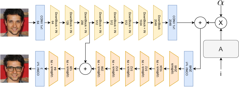
Figure 1: Generator architecture. Numbers correspond to the output channels of each block.

Residual Blocks.

Each DownBlock and UpBlock has a residual block followed by a downsampling and upsampling layer, respectively. For downsampling, we use average pooling and for upsampling, we use nearest-neighbor. This operation is denoted as Resample in Fig. 2. The architecture of the residual block is given in Fig. 2.

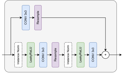
Figure 2: Architecture for the residual blocks.

Discriminator.

The architecture of the discriminator is given in Fig. 3. It also employs an architecture with decreasing resolution and increasing channel size. Just like the generator, we build our discriminator with channel sizes of {64, 64, 128, 256, 512, 512, 512, 1024, 2048}, that reduces the feature map dimensions to 1x1. At the end, we concatenate the extracted style $\alpha_{t}$ from the input image to this latent code and apply a 1x1 convolution. This final convolution is specific to each tag-attribute pair so that the model can use this information.

Figure 3: Architecture of the discriminator. Discriminator takes an input image and processes it with downsampling blocks with increased number of channels. Towards the end, the extracted feature map with 1x1 feature dimensions is concatenated with the scale of the input image. As we perform scale extraction for the image in the cycle-translation path, no additional scale extraction is needed.

Hyperparameters.

For training our framework, we set the following parameters; $\lambda_{a}=1$, $\lambda_{rec}=1.5$, $\lambda_{s}=1$, $\lambda_{o}=1$ and $\lambda_{sp}=0.05$. We use a learning rate of $10^{-4}$ and train our model for 500K iterations with a batch size of 8 on a single GPU. For the feature encoding and feature directions in matrix $A$, we use a 2048 dimensional vector representation same as the channel size of the last convolutional layer from the encoder.

Appendix 0.B Additional Results

We provide additional qualitative results of our method in Fig. 4, 5, 6, 7, 8, and 9.

Figure 4: Smile tag manipulation results. First and third rows show input images. Second and forth rows show image translation results.

Figure 5: Glasses tag manipulation results. First and third rows show input images. Second and forth rows show image translation results.

Figure 6: Gender tag manipulation results. First and third rows show input images. Second and forth rows show image translation results.

Figure 7: Bangs tag manipulation results. First and third rows show input images. Second and forth rows show image translation results.

Figure 8: Age tag manipulation results. First and third rows show input images. Second and forth rows show image translation results.

Figure 9: Hair tag manipulation results. First and third rows show input images. Second and forth rows shows image translation results.

Appendix 0.C Analysis of Encoded Scales

We explore the encoded scales from reference images, $\alpha_{t}$. These scales are supposed to provide information about the attribute of the image (whether person smiles or not) and its intensity (how big the smile is). We plot the histograms of $\alpha_{t}$ values from validation images for eyeglasses and smile tags and use orange and blue colors depending on their ground-truth tags from the validation list as shown in Fig. 10. We find that for eyeglasses, $\alpha_{t}$ values are disentangled from each other for eyeglasses positive and negative classes. For smiling tag, they are mostly disentangled with a small intersection. Next, we visualize the samples for smiling tag.

(a)

(b)

Figure 10: Histogram of $\alpha_{t}$ distribution of eyeglasses and smile tags.

Fig. 11 shows a visualization of validation images plotted based on their $\alpha_{t}$ values extracted for smiling tag. We visualize few samples from each bin from the histogram above with the same frequency as the histogram value. The visualization shows that $\alpha_{t}$ values encode the intensity of the smile. The most left samples have large smiles, and the most right samples look almost angry. On the other hand, the images in the middle space are confusing ones. We also observe many wrong labeling in the validation images by going through the middle space.

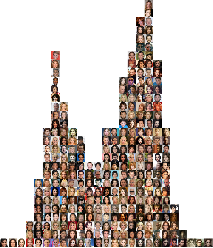
Figure 11: Training images plotted based on their $\alpha_{t}$ values extracted for smiling tag.