On Weak Lensing Response Functions

Abstract

We introduce the response function (RFs) approach to model the weak lensing statistics in the context of separate universe formalism. Numerical results for the RFs are presented for various semi-analytical models that includes perturbative modelling and variants of halo models. These results extend the recent studies of the Integrated Bispectrum (IB) and Trispectrum to arbitrary order. We find that due to the line-of-sight (los) projection effects, the expressions for RFs are not identical to the squeezed correlation functions of the same order. We compute the RFs in three-dimensions (3D) using the spherical Fourier-Bessel (sFB) formalism which provides a natural framework for incorporating photometric redshifts, and relate these expressions to tomographic and projected statistics. We generalise the concept of $k$-cut power spectrum to $k$-cut response functions. In addition to response function for high-order spectra, we also define their counterparts in real space, since they are easier to estimate from surveys with low sky-coverage and non-trivial survey boundaries.

1 Introduction

The current generation of weak lensing surveys [1, 2] including the Subaru Hypersuprimecam survey(HSC) [3], Dark Energy Survey(DES)[4], Dark Energy Spectroscopic Instruments (DESI), Prime Focus Spectrograph, KiDS[5] are already able to put cosmological constraints that are competitive with recent Cosmic Microwave Background surveys. The near-future Stage-IV large scale structure (LSS) surveys such as Euclid[6], Rubin Observatory[7] and Roman Space Telescope[8] will improve the constraints by an order-of-magnitude and provide answers to many of the questions that cosmology is facing. These will provide answers to many outstanding cosmological questions, including but not limited to, nature of dark matter (DM), dark energy (DE), possible modifications of General Relativity (GR) on cosmological scales [9, 10] and the sum of the neutrino masses [11].

Weak lensing observations target the relatively low-redshift ($z\sim 1$) universe and small scales where the perturbations are in the nonlinear regime and their statistics are non-Gaussian [1, 12, 2]. Indeed, understanding higher-order statistics is important as they can significantly reduce the degeneracy in cosmological parameters[13]. Nevertheless, higher-order statistics beyond the bispectrum and trispectrum are known to be difficult to model analytically, and in perturbation theory higher-order contributions becomes increasingly intractable as the order increases. Analytical modelling of the weak lensing three-point correlation function was initiated in real-space in [13, 14], and parallel development in the harmonic domain was initiated in [15, 16]. For early detection of non-Gaussianity see [17].

Another strand of work has involved designing and optimising estimators of non-Gaussianity. The numerical estimators are computationally demanding to implement. In addition, higher-order estimators are typically noise-dominated on small scales and cosmic variance dominated on large scales. A large number of simulations are required to accurate characterization [18]. Many different estimators have recently been proposed which probe the higher-order statistics of weak lensing maps [19]. These include the well-known real-space one-point statistics such as the cumulants [20] or their two-point correlators also known as the cumulant correlators as well as the associated PDF [21] and the peak-count statistics [22]. In the harmonic domain the estimators such as the Skew-Spectrum[23], Integrated Bispectrum [24] kurt-spectra [25], morphological estimator [26], integrated trispectrum [27], Betti number [28], extreme value statistics [29], position-dependent PDF [30], density split statistics [31], response function formalism [32], statistics of phase [34, 35, 36], estimators for shapes of the lensing bispectrum [33] are some of the statistical estimators and formalism recently considered by various authors in the context of understanding cosmological statistics in general and weak lensing in particular. In recent years approaches based on machine learning have also been employed [37].

In recent years a novel technique known as a Separate Universe (SU) formalism was developed by many authors (see e.g. [38] for a complete list of references). The primary aim of this paper is to introduce the SU formalism in the study of a specific weak lensing statistic known as the response function. We will use this statistic to probe non-Gaussianity in weak lensing maps in projection (2D) as well as in three dimensions (3D). We will show due to projection effects, the response functions are not identical to the higher-order correlation functions in the squeezed limit but are closely related.

This paper is arranged as follows. In §1 we introduce our notations, next, in 2 we detail the formalism of response functions in the context of separate Universe formalism for weak lensing convergence. In §4 we develop the response functions for the weak lensing. The response functions for higher-order cross-correlations against CMB is given in §LABEL:sec:cross. Response functions for $k$-cut correlation functions are presented in §5. The results are discussed in §6 and conclusions and future prospects are presented in §7.

The cosmological model parameters used are the Planck2015 best-fit flat $\Lambda$CDM model [39]: $h=0.6727$, $\Omega_{b}=0.0492$, $\Omega_{m}=0.3156$, $\Omega_{\Lambda}=0.6844$, $n_{s}=0.9645$ and $\sigma_{8}=0.831$.

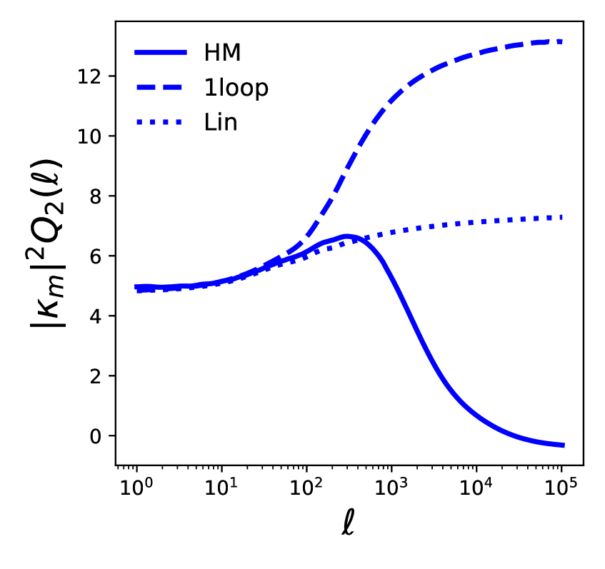
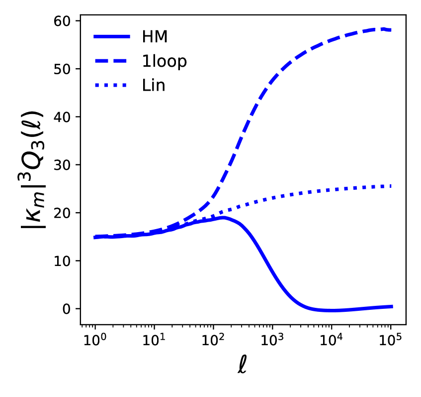
Figure 1: The response functions $|\kappa_{m}|^{N}Q_{N}$ defined in Eq.(3.11) are shown. From left to right panels depict $N=1,2$ and $N=3$. The source redshift is $z_{s}=1$. Various line styles correspond to different analytical models, linear, one-loop and halo model as indicated (see text for details).

2 Weak Lensing Convergence in Projection

The projected (2D) weak lensing convergence $\kappa$ is a line-of-sight integration of the underlying three-dimensional (3D) cosmological density contrast $\delta$. The $\kappa({{\bm{\theta}}})$ at a position ${\bm{\theta}}$ can be expressed as follows:

$$\kappa({\bm{\theta}},z_{s}):=\int_{0}^{r_{s}}drW(r)\delta(r,{\bm{\theta}});$$ (2.1a)

$$:={3\Omega_{\rm M}\over 2}{H_{0}^{2}\over c^{2}}a^{-1}{d_{A}(r)d_{A}({r_{s}-r})\over d_{A}(r_{s})}.$$ (2.1b)

We will suppress the variables $r_{s}$ unless we consider the case where the sources are not confined in a single source plane. Here $d_{A}(r)$ is the comoving angular diameter distance at a comoving distance $r$, i.e., $\kappa({\bm{\theta}},z_{s})\equiv\kappa({\bm{\theta}})$ and $W(r.r_{s})\equiv W(r)$. The kernel $W(r)$ encodes geometrical dependence; $a$ is the scale factor, $H_{0}$ is the Hubble constant and $\Omega_{M}$ is the cosmological density parameter. $d_{A}(r)$ and $d_{A}(r_{s})$ are comoving angular diameter distances at a comoving distances $r$ and $r_{s}$. We have assumed all sources to be at a single source plane at a distance $r_{s}$. The projected lensing power spectrum ${\cal C}_{\ell}$ is given in the Limber and Born approximations by:

$${\cal C}_{\ell}=\int_{0}^{r_{s}}dr{W^{2}(r)\over d_{A}^{2}(r)}P_{\delta}\left({{\ell}\over d_{A}(r)};r\right).$$ (2.2)

The tomographic power spectrum ${\cal C}^{ij}_{\ell}$ is given by restricting the line-of-sight integration for sources in a particular estimated redshift bins (labelled by $i,j$):

$${\cal C}^{ij}_{\ell}=\int_{0}^{r_{s}}dr{W_{i}(r)W_{j}(r)\over d_{A}^{2}(r)}P_{\delta}\left({{\ell}\over d_{A}(r)};r\right).$$ (2.3)

the kernels $W_{i}$ and $W_{j}$ can be obtained by replacing $r_{s}$ in Eq.(2.1b) respectively by $r_{si}$ and $r_{j}$. The upperlimit of integration will be $r_{s}=min(r_{si},r_{sj})$.

Throughout, we assume that all sources are at a single source redshift distribution. For a distribution of source redshifts there is a further radial integration.

$${\cal C}_{\ell}=\int_{0}^{r_{s}}dr{{\hat{W}}^{2}(r)\over d_{A}^{2}(r)}P_{\delta}\left({{\ell}\over d_{A}(r)};r\right).$$ (2.4)

$$\kappa(\bm{\theta})=\int_{0}^{\infty}n(z_{s}){\kappa(\bm{\theta},z_{s})dz_{s}};\quad=\int_{0}^{r_{max}}dr\hat{W}(r)\delta(r);$$ (2.5)

$$\hat{W}(r)=\int^{\infty}_{z_{s}}dz_{s}W(r,r_{s})n(z_{s}).$$ (2.6)

The integral along the radial direction takes into account contribution from individual source planes and $n(z_{s})$ number density of sources at a source redshift $z_{s}$. We ignore the discreteness effect.

3 Separate Universe Formalism and Response Functions in Projection

In a SU formalism an infinite wavelength adiabatic perturbation $\delta_{\rho}$ is absorbed in the background matter density by redefining the cosmological parameters (e.g., [40, 41]). We will denote the comoving coordinate, scale-factor, comoving wave number, and power spectrum respectively as ${\bf x}$, $a(t)$, $k$ and $P(k)$. The corresponding quantities in the modified cosmology will be denoted as $\tilde{\bf x}$, $\tilde{a}(t)$, $\tilde{k}$ and $\tilde{P}(\tilde{k})$. We will also introduce $\delta_{a}$ and $\delta_{\rho}$ the Lagrangian and Eulerian perturbation as follows:

$${\bf x}a(t)=\tilde{\bf x}{\tilde{a}}(t);\quad 1+\delta_{a}={\tilde{a}(t)\over a(t)}$$ (3.1a)

$$(1+\delta_{\rho})=(1+\delta_{a})^{-3}.$$ (3.1b)

$$\tilde{\Omega}_{M}\tilde{h}^{2}=\Omega_{M}h^{2}$$ (3.1c)

$$\tilde{x}=(1+\delta_{a})^{-1}x;\quad\quad\tilde{k}=(1+\delta_{a})k.$$ (3.1d)

Following the derivation in [38] we can expand $\delta_{a}$ and $\delta_{\rho}$ in terms of the linear overdensity $\delta_{L}=D_{+}\delta_{L0}$: The evolution of $\delta_{a}$ and $\delta_{\rho}$ in the fiducial cosmology can be solved using a spherical collapse model. The equations are further simplified by an Einstein de Sittter (EdS) cosmology. The accuracy of such approximations have been tested and was found to be better than a few percents.

$$\delta_{a}=\sum_{n=1}^{\infty}e_{n}[\delta_{L}]^{n};\quad\delta_{\rho}=\sum_{n=1}^{\infty}f_{n}[\delta_{L}]^{n};$$ (3.2a)

$$e_{i}=\Big{\{}-{1/4},-{1/21},-{23/1701},\cdots\Big{\}}$$ (3.2b)

$$f_{i}=\Big{\{}1,17/21,341/567,\cdots,\Big{\}}$$ (3.2c)

The power spectrum in modified cosmology will be denoted as ${\tilde{P}}_{\delta}$ and in the fiducial cosmology by $P_{\delta}$ are related by the following expression:

$$P_{\delta}(k|\delta_{L})=[1+\delta_{\rho}]{\tilde{P}}_{\delta}([1+\delta_{a}]k).$$ (3.3)

The growth-only response function is denoted by $G_{n}$ and the total response function by $R_{n}$.

$${\tilde{P}}_{\delta}(k,t)=\sum_{n=0}^{\infty}{\delta_{L}^{n}\over n!}G_{n}(k,t)\,P_{\delta}(k,t);$$ (3.4a)

$${P}_{\delta}(k,t|\delta_{L})=\sum_{{{\color[rgb]{0,0,0}n=0}}}^{\infty}{\delta_{L}^{n}\over n!}R_{n}(k,t)\,P_{\delta}(k,t).$$ (3.4b)

The nth-order response function for the density contrast is given by the nth-order derivative of the power spectrum with the linearly extrapolated overdensity $\delta_{L0}$. A normalisation is also introduced by the power spectrum which renders the response function dimensionless.

$$R_{n}(k,t)={1\over P_{\delta}(k,t)}{d^{n}P_{\delta}(k,t|\delta_{L})\over d\delta^{n}_{L}(t)}\Big{|}_{\delta_{L}=0};$$ (3.5a)

$$G_{n}(k,t)={1\over P_{\delta}(k,t)}{d^{n}{\tilde{P}}_{\delta}(k,t)\over d\delta^{{\color[rgb]{0,0,0}n}}_{L}(t)}\Big{|}_{\delta_{L}=0}.$$ (3.5b)

The response functions can be recovered by Taylor expanding Eq(3.3). Next, we will focus on response function for the power spectrum of the weak lensing convergence. We will express these response functions in terms of the 3D response function for matter power spectrum.

The 2D power spectrum is given by:

$${\cal{C}}_{\ell}(\kappa_{L})=\int_{0}^{r_{s}}dr{{{\color[rgb]{0,0,0}W}}^{2}(r)\over{d^{2}_{A}}(r)}P_{\delta}\left({\ell\over r};r\Big{|}\delta_{L}\right).$$ (3.6)

We will refer to this as the local angular power spectrum. The global angular power spectrum is recovered by taking $\delta_{L}=0$ which leads to $\kappa_{L}=0$ and we recover Eq.(2.4).

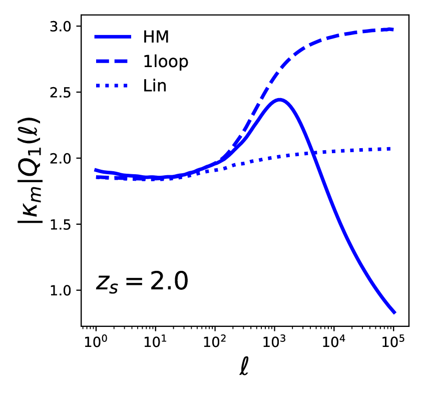
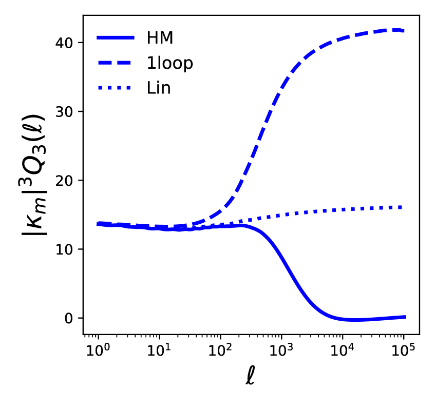
Figure 2: Same as Fig.1 but for source redshift $z_{s}=2$.

Using Eq.(3.4a) we can write:

$${\cal C}_{\ell}(\kappa_{L})=\sum_{n=0}^{\infty}{1\over n!}[\delta_{L0}]^{n}\int_{0}^{r_{s}}dr{{{\color[rgb]{0,0,0}W}}^{2}(r)\over{d^{2}_{A}}(r)}R_{n}\left({\ell\over d_{A}(r)},r\right)[D_{+}(r)]^{n}P_{\delta}\left({\ell\over d_{A}(r)},r\right).$$ (3.7)

Using the following notation:

$$\kappa_{L}=\delta_{L}|\kappa_{m}|;\quad\kappa_{m}=-\int_{0}^{r_{s}}drD_{+}(r)\,{{\color[rgb]{0,0,0}W}}(r);$$ (3.8)

where $\delta_{L}$ is the local over(under)-density and corresponding projected convergence is $\kappa_{L}$

$${\cal C}_{\ell}(\kappa_{L})=\sum_{n=0}^{\infty}{1\over n!}\left[{\kappa_{L}\over|\kappa_{m}|}\right]^{n}\int_{0}^{r_{s}}dr{{W}^{2}(r)\over{d^{2}_{A}}(r)}R_{n}\left[{\ell\over d_{A}(r)},r\right][D_{+}(r)]^{n}P_{\delta}\left({\ell\over d_{A}(r)},r\right).$$ (3.9)

If we define the response functions for the 2D as ${\cal Q}_{n}(\ell)$ we can write:

$${\cal C}_{\ell}(\kappa_{L})=\sum_{n=0}^{\infty}{1\over n!}\;{\cal Q}_{n}(\ell)\;{\kappa^{n}_{L}}\;{\cal C}_{\cal\ell}$$ (3.10)

Comparing Eq.(4.8) with Eq.(3.9) we deduce that:

$$Q_{n}(\ell)={1\over{\cal C}_{\ell}}{1\over|\kappa_{m}|^{n}}\int_{0}^{r_{s}}dr{{W}^{2}(r)\over{d^{2}_{A}}(r)}R_{n}\left[{\ell\over d_{A}(r)},r\right][D_{+}(r)]^{n}P_{\delta}\left({\ell\over d_{A}(r)},r\right).$$ (3.11)

The respone function for cross-correlation of two different tomographic bins denoted by indices $i$ and $j$ can be derived similarly. We start from the definition of local cross-spectra:

$${\cal{C}}^{ij}_{\ell}(\kappa_{LX})=\int_{0}^{r_{s}}dr{{W}^{i}(r){W}^{j}(r)\over{d^{2}_{A}}(r)}P_{\delta}\left({\ell\over r};r\Big{|}\delta_{L}\right)\quad\;{\kappa_{LX}}\equiv[{\kappa_{im}}{\kappa_{jm}}]^{n/2}$$ (3.12)

We will later define the local cross-spectra in terms of $\kappa_{LX}$ which is a geometric mean of $\kappa_{mi}$ and $\kappa_{mj}$ i.e. $\kappa_{m}$ of the tomographic bins $i$ and $j$ respectively. Mathematically,

$$\kappa_{iL}=\delta_{L}|\kappa_{im}|;\quad\kappa_{im}=-\int_{0}^{r_{s}}drD_{+}(r)\,W_{i}(r);$$ (3.13)

The response functions ${\cal Q}^{ij}_{n}(\ell)$ for cross-spectra involving two tomographic is expressed as:

$${\cal C}^{ij}_{\ell}(\kappa_{LX})=\sum_{n=0}^{\infty}{1\over n!}\;{\cal Q}^{ij}_{n}(\ell)\;{\kappa^{n}_{LX}}{\cal C}^{ij}_{\cal\ell};$$ (3.14)

Combining Eq.(5.5) and Eq.(3.12)

$$Q^{ij}_{n}(\ell)={1\over{\cal C}^{ij}_{\ell}}{1\over|\kappa_{LX}|^{n}}\int_{0}^{r_{s}}d\tilde{r}{{W}^{i}(r){W}^{j}(r)\over{d^{2}_{A}}(r)}R_{n}\left[{\ell\over d_{A}(r)},r\right][D_{+}(r)]^{n}P_{\delta}\left({\ell\over d_{A}(r)},r\right).$$ (3.15)

Throughout, we have used Limber approximation. The FFTlog based approach is often used to go beyond the Limber approximation [42] in the modelling of projected power spectrum. It is possible to incorporate a similar method to model the low-$\ell$ behaviour of the response functions. The expressions above are derived for single source plane. For generalisation to a source distribution specified by $n(z)$ we need to replace $W(z)$ in Eq.(3.6), Eq.(3.11) and other equations by $\hat{W}(z)$ as defined in Eq.(2.6). The definition of $\kappa_{m}$ in Eq.(3.8) similarly will have to be modified.

Next, from [38] we have used the following expressions:

$$R_{0}(k)=1;$$ (3.16a)

$$R_{1}(k)=f_{1}+e_{1}{kP^{\prime}(k)\over P(k)}+G_{1}(k);$$ (3.16b)

$${1\over 2}R_{2}(k)=f_{2}+e_{2}{kP^{\prime}(k)\over P(k)}+e_{1}^{2}{k^{2}P^{{{\color[rgb]{0,0,0}\prime\prime}}}(k)\over 2P(k)}+{1\over 2}G_{2}{(k)}+f_{1}G_{1}(k)$$

$$\quad+{{\color[rgb]{0,0,0}f_{1}}}e_{1}{kP^{\prime}(k)\over P(k)}+e_{1}{kP^{\prime}(k)\over P(k)}G_{1}(k)+e_{1}kG^{\prime}_{1}(k);$$ (3.16c)

$${1\over 6}{R_{3}(k)}=f_{1}{{\color[rgb]{0,0,0}G_{1}}}(k)e_{1}{kP^{\prime}(k)\over P(k)}+f_{3}+{{{\color[rgb]{0,0,0}G_{3}}}(k)\over 6}+e_{3}{kP^{\prime}(k)\over P(k)}+f_{1}{G_{2}(k)\over 2}+f_{1}e_{2}{kP^{\prime}(k)\over P(k)}$$

$$+f_{1}e_{1}^{2}{k^{2}P^{\prime\prime}(k)\over 2P(k)}+f_{2}G_{1}(k)+f_{2}e_{1}{kP^{\prime}(k)\over P(k)}+(f_{1}e_{1}+e_{2})kG_{1}^{\prime}(k)+e_{1}^{2}{k^{2}G_{1}^{{\color[rgb]{0,0,0}\prime\prime}}(k)\over 2}$$

$$+e_{1}k{G^{\prime}_{2}(k)\over 2}+e_{1}^{2}{kP^{\prime}(k)\over P(k)}{kG^{\prime}_{1}(k)}+e_{1}^{3}{k^{3}P^{\prime\prime\prime}(k)\over 6P(k)}+2e_{1}e_{2}{k^{2}P^{\prime\prime}(k)\over 2P(k)}$$

$$+e_{1}{kP^{\prime}(k)\over P(k)}{G_{2}(k)\over 2}+G_{1}(k)\left(e_{2}{kP^{\prime}(k)\over P(k)}+e_{1}^{2}{k^{2}P^{\prime\prime}(k)\over 2P(k)}\right).$$ (3.16d)

In our notation $\hat{D}_{+}(t)$ represents the linear growth rate. The growth only response functions, denoted as $G_{n}$, takes a particularly simpler form when computed using linear theory.

Notice that the response functions ${R_{n}(k)}$ take a rather simpler form when we approximate the power spectrum locally as a power law. In this case, we can write $P(k)\propto k^{n}$ which leads us to $kP^{\prime}(k)/P(k)=n$ and $k^{2}\,P^{\prime\prime}(k)/P(k)=n(n-1)$, and to a good approximation the growth rate $G(k)$ is scale-independent.

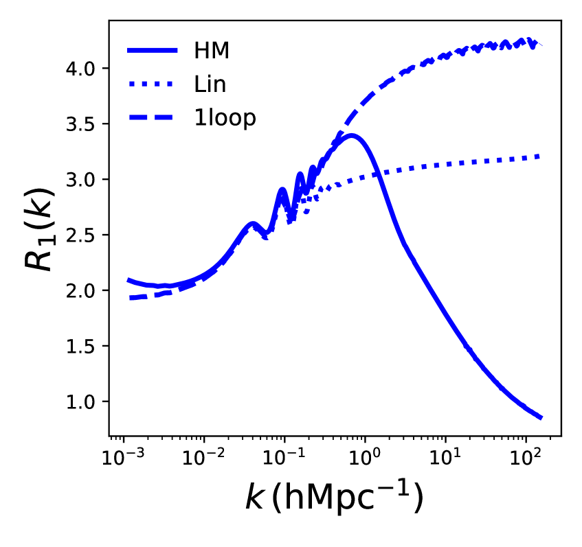
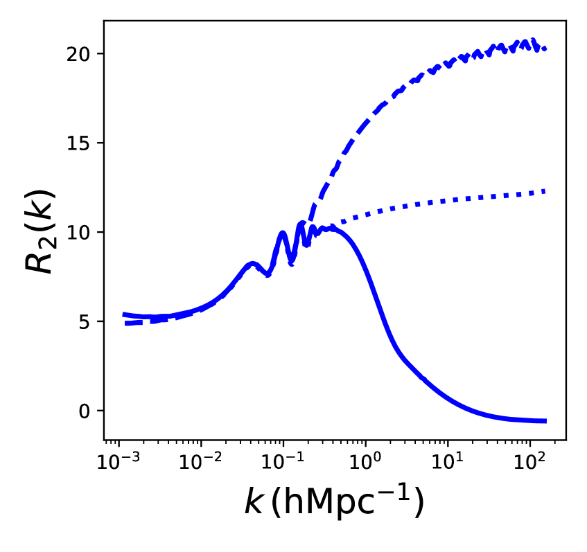
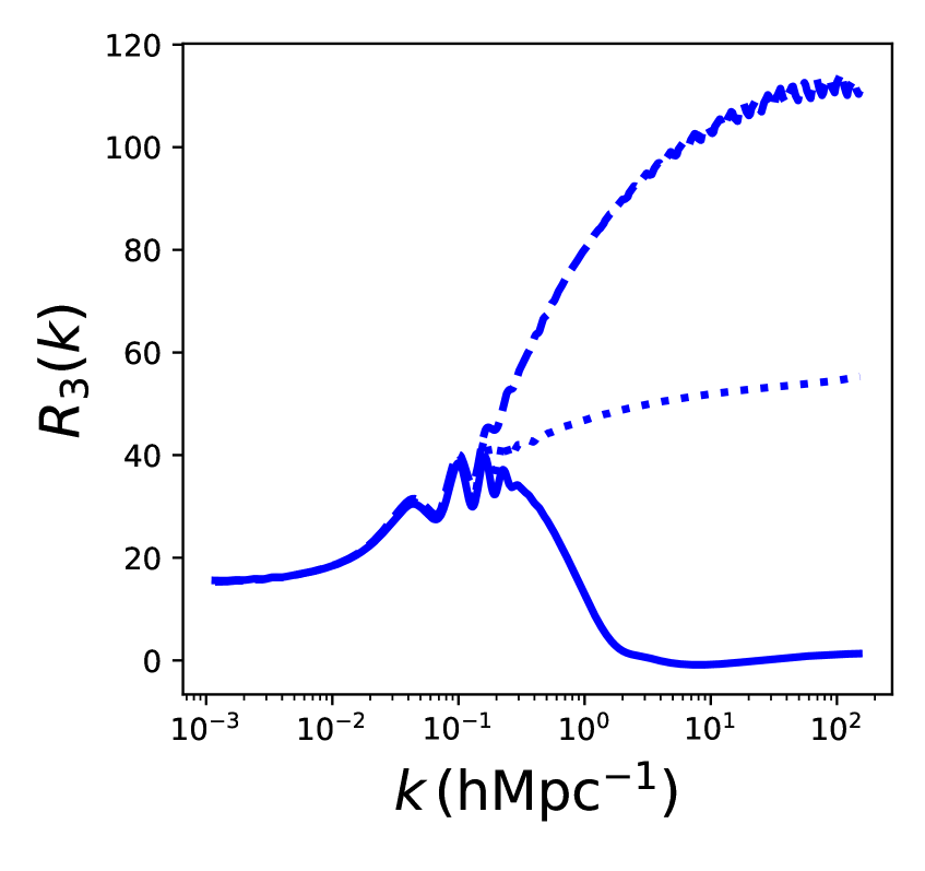
Figure 3: The response functions $R_{N}$ defined in Eq.(3.16b)-Eq.(3.16d) are shown. From left to right panels depict $N=1,2$ and $N=3$. The simulation redshift is at $z_{s}=1$. Various line styles correspond to different analytical models, linear, one-loop and halo model as indicated (see text for details).

$$G_{n}={1\over D_{+}^{2}}{d^{n}{{\color[rgb]{0,0,0}\tilde{D}}}_{+}^{2}\over d\delta^{n}_{L}}\Big{|}_{\delta_{L}=0};$$ (3.17a)

$$\tilde{D}_{+}(t)=D_{+}(t){{\color[rgb]{0,0,0}\sum_{n=0}^{\infty}}}{{\color[rgb]{0,0,0}g}}_{n}[\delta_{L}]^{n};$$ (3.17b)

$${{\color[rgb]{0,0,0}g_{n=0,1,2,3,4}=\left\{1,{13/21},{71/189},\cdots\right\};}}$$ (3.17c)

$$G_{n=0,1,2,3,4}=\left\{1,{26/21},{3002/1323},\cdots\right\}.$$ (3.17d)

In the linear theory Eq.(3.3) takes the following form for the linear power spectrum local $P_{L}$ and the fiducial power spectrum $P_{lin,fid}$:

$$P_{L}(k,t|\delta_{L})=(1+\delta_{\rho}(t))\left({\tilde{D}_{+}(t)\over D_{+}(t)}\right)^{{\color[rgb]{0,0,0}2}}{\tilde{P}}_{L,fid}(k,t).$$ (3.18)

Next, we turn our attention to a perturbative quasilinear calculation of response functions. The response functions for the density contrast $\delta$ are related to the angle averaged squeezed limits of correlation functions $S^{\delta}_{N-2}$ defined as follows:

$$S^{\delta}_{N-2}(k,k^{\prime},k_{1},\cdots k_{N-2})=\int{d{\hat{\Omega}}_{1}\over 4\pi}\cdots\int{d{\hat{\Omega}}_{N-2}\over 4\pi}\langle\delta({\bf k})\delta({\bf k}^{\prime})\delta({\bf k}_{1})\cdots\delta({\bf k}_{N-2})\rangle^{\prime}.$$ (3.19a)

$$R_{N-2}(k)=\lim_{k_{i}\rightarrow 0}{S_{N-2}(k,k^{\prime},k_{1},\cdots k_{N-2})\over P_{L}(k_{1})\cdots P_{L}(k_{N-2})}$$ (3.19b)

Here, $d\hat{\Omega}_{i}=\sin\theta_{i}d\phi_{i}$. The angles $\hat{\Omega}_{i}=(\theta_{i},\phi_{i})$ are the angles associated with wave vector${\bf k}$ and $P_{L}$ is the linear power spectrum. We have used following shorthand notation above:

$$\langle\delta({\bf k})\delta({\bf k}^{\prime})\delta({\bf k}_{1})\cdots\delta({\bf k}_{N-2})\rangle^{\prime}=(2\pi)^{3}\delta_{\rm 2D}({\bf k}_{1})+\cdots+{\bf k}_{N-2})$$

$$\,\times\,\langle\delta({\bf k})\delta({\bf k}^{\prime})\delta({\bf k}_{1})\cdots\delta({\bf k}_{N-2})\rangle$$ (3.20)

Here, $\delta_{\rm nD}$ represents the $n$-dimensional Dirac delta function. In case of 2D convergence or $\kappa$similarly we have:

$$S^{\kappa}_{N-2}(\ell,\ell^{\prime},\ell_{1},\cdots\ell_{N-2})=\int{d\theta_{1}\over 2\pi}\cdots\int{d\theta_{1}\over 2\pi}\langle\kappa({\bf{l}})\kappa({\bf{l}}^{\prime})\kappa({\bf{l}}_{1})\cdots\kappa({\bf{l}}_{N-2})\rangle^{\prime}.$$ (3.21a)

$$Q_{N-2}(\ell)=\lim_{\;\ell_{i}\rightarrow 0}{S^{\kappa}_{N-2}(\ell,\ell^{\prime},\ell_{1},\cdots\ell_{N-2})\over{\cal C}^{\kappa}_{\ell_{1}}\cdots{\cal C}^{\kappa}_{\ell_{N-2}}}.$$ (3.21b)

In the above expression $$\theta_{i} {\bf{l}}_{i} \ell_{i}=|{\bf{l}}_{i}| {\cal C}^{\kappa}_{\ell_{1}}$$ is the polar angle of the vector and . The power spectrum is the linear convergence power spectrum for the same source distribution. The following notation was used:

$$\langle\kappa({\bf{l}})\kappa({\bf{l}}^{\prime})\kappa({\bf{l}}_{1})\cdots\kappa({\bf{l}}_{N-2})\rangle^{\prime}=(2\pi)^{2}\delta_{\rm 2D}({\bf{l}}_{1}+\cdots+{\bf{l}}_{N-2})$$

$$\quad\quad\quad\quad\quad\quad\quad\quad\quad\quad\,\times\,\langle\kappa({\bf{l}})\kappa({\bf{l}}^{\prime})\kappa({\bf{l}}_{1})\cdots\kappa({\bf{l}}_{N-2})\rangle$$ (3.21c)

The projected higher-order squeezed spectra are not identical to the projected response functions of same order. See for exact perturbative results in Appendix-§A

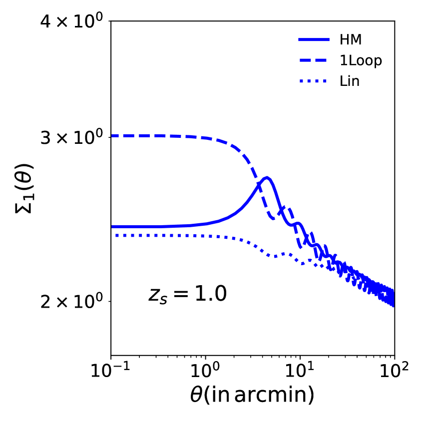
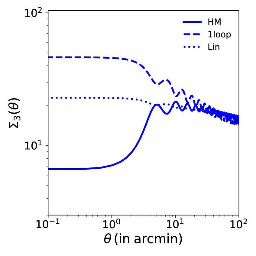
Figure 4: The response functions $\Sigma_{N}$ defined in Eq.(3.29c) are shown for the source redshift $z_{s}=1.0$. From left to right panels depict $N=1,2$ and $N=3$. Various line styles correspond to different analytical models, linear, one-loop and halo model as indicated.

3.1 Beyond Linear Theory - Loop Corrections

In the standard perturbation theory (SPT) the power spectrum at a redshift $z$ has the following expression (e.g., [12]):

$$P^{\rm SPT}(k)=D_{+}^{2}P_{L}(k)+D_{+}^{4}P^{\rm{1-loop}}(k)+D_{+}^{6}P^{\rm{2-loop}}(k)+\cdots$$ (3.22)

Here $P^{\rm{1-loop}}$ $P^{\rm{2-loop}}$ denote loop-level corrections to the linear power spectrum $P_{L}$. In the previous section we used the linear power spectrum for computing the response functions. Perturbative corrections to the linear theory as given in Eq.(3.22) can improve these predictions when used in association with Eq.(3.16c)-Eq.(3.16d).

3.2 Halo Model Response Functions

We introduce the following notation:

$$I_{m}^{n}(k_{1},\cdots,k_{m})\equiv\int d\ln Mn(\ln M)\left({M\over\bar{\rho}}\right)^{{\color[rgb]{0,0,0}m}}b_{n}(M)u(M|k_{1})\cdots u(M|k_{m}).$$ (3.23)

Here $b_{n}(M)$ is the $n$-th order bias and $u(M|k_{1})$ is the Fourier transform of the halo profile and $k_{i}$ are the wave numbers. The power spectrum in the halo model has two contributions known as the 1-halo and 2-halo contribution $P_{1h}(k)$ and $P_{1h}(k)$ [43]:

$$P_{\rm HM}(k)=P_{2h}(k)+P_{1h}(k);$$ (3.24a)

$$P_{2h}(k)=[I^{1}_{1}(k)]^{2}P_{\rm L}(k);\quad P_{1h}(k)=I_{2}^{0}(k,k).$$ (3.24b)

Following Ref.([59]) we can write the position-dependent 1-halo contribution as [43]:

$$P_{1h}(k,t|\delta_{L0})=\sum_{n=0}^{\infty}{1\over n!}I_{2}^{n}(k,k,t)[{\hat{\delta}_{L}}]^{n}.$$ (3.25a)

The 2-halo contribution is similarly given by [43]:

$$P^{2h}(k,t,|\delta_{L0})=\left(\sum^{\infty}_{n=0}{1\over n!}f_{n}[\delta_{L}]^{n}\right)[{\hat{\delta}_{L}}]^{n}$$

$$\times\left(\sum^{\infty}_{n=0}{1\over n!}{{\color[rgb]{0,0,0}I_{1}^{n+1}(k,t)}}[\delta_{L}]^{n}\right)P_{lin}\left[\left(\sum^{\infty}_{n=0}{1\over n!}{{\color[rgb]{0,0,0}e_{n}}}[\delta_{L}]^{n}\right)k\right].$$ (3.26)

Finally, the response functions in the halo model are given by [38]:

$$R_{1}^{\rm HM}(k)=\Big{[}f_{1}+2g_{1}+e_{1}{d\ln P(k)\over d\ln k}\Big{]}P_{2h}(k,t)+I^{1}_{2}(k,k,t);$$ (3.27a)

$$R_{2}^{\rm HM}(k)=\Big{[}2f_{2}+2f_{1}g_{1}+(f_{1}+2g_{1}{{\color[rgb]{0,0,0})e_{1}}}{d\ln P(k)\over d\ln k}$$

$$\quad+2g_{1}^{2}+4g_{2}+2e_{2}{d\ln P(k)\over d\ln k}+e_{1}^{{\color[rgb]{0,0,0}2}}{1\over P}{d^{2}\ln P(k)\over d(\ln k)^{2}}\Big{]}P_{2h}(k,t)+I^{2}_{2}(k,k,t).$$ (3.27b)

The $n-$th order response function we have derived correspond to the Lagrangian density contrast $\delta_{a}$ and is generally denoted as $R^{L}_{n}$ to distinguish it from the Eulerian response function related to density contrast $\delta_{\rho}$. The conversion between the Lagrangian and Eulerian response functions is given by:

$$R_{1}^{E}(k)=R^{L}_{1}(k);$$ (3.28a)

$$R_{2}^{E}(k)=R_{2}^{L}(k)−2f_{2}R^{L}_{1}(k);$$ (3.28b)

$$R_{3}^{E}(k)=R_{3}^{L}(k)−6f_{2}R^{L}_{2}(k)+6(2f_{2}^{2}−f_{3})R_{1}(k).$$ (3.28c)

We have computed the Lagrangian projected response functions $Q_{N}$ by using the 3D Lagrangian response function $R^{L}_{1}(k)$. However, the projected Eulerian response functions can be computed using $R^{E}_{1}(k)$ in a straight forward manner.

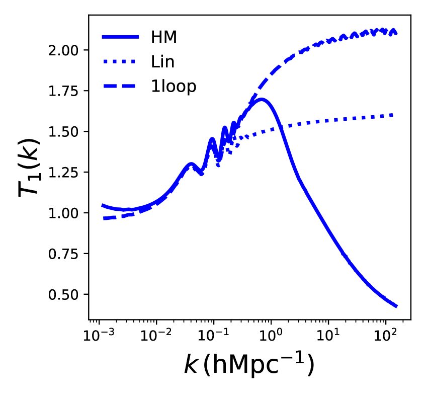
Figure 5: The parameters $T_{N}$ for redshift $z=0$ defined in Eq.(4.4a) - Eq.(4.4c) are plotted as a function the wave number $k$. From left to right panels depict $N=1,2,3$. Various line styles correspond to different analytical models, linear, one-loop and halo model as indicated (see text for details).

In addition to the perturbation theory and halo model based results, the response functions can also be computed using the Effective Field Theory (EFT) predictions for the power spectrum [44].

3.3 Response Functions for Two-point Correlation Function

In this section we will extend the results derived above to real space and derive the response functions for the two-point correlation function: $\xi(\theta_{12})\equiv\langle\kappa({\bm{\theta}})\kappa(\bm{\theta+\theta_{12}})\rangle$. Isotropy and homogeneity dictates $\xi(\theta_{12})$ only depends on the separation $\theta_{12}=|\bm{\theta_{12}}|$. For surveys with small sky-coverage and masks with non-trivial topology, response functions defined for two-point correlation function are easier to implement [48, 47, 49]. We begin by defining the local estimate of the two-point correlation function (2PCF) $\xi(\theta_{12})$ as

$$\xi(\theta_{12}|\kappa_{L})={1\over 4\pi}\sum_{\ell=0}^{\ell_{max}}(2\ell+1)P_{\ell}(\cos\theta_{12}){\cal C}_{\ell}(\kappa_{L}).$$ (3.29a)

Here $$P_{\ell} \ell \xi(\theta) {\cal C}_{\ell}(\kappa_{L}) {\cal C}_{\ell} \Sigma_{n} \xi(\theta|\kappa_{L}) \kappa_{L}$$ is the Legendre polynomial of order . The corresponding global two-point correlation function can be recovered by replacing the local power spectrum with its global counterpart . The n-th order response function as the n- order derivative of the local correlation function w.r.t the local convergence :

$$\Sigma_{n}(\theta_{12})={1\over\xi(\theta_{12})}{d^{n}\xi(\theta_{12}|\kappa_{L})\over d\kappa^{n}_{L}}.$$ (3.29b)

Using Eq.(4.8) in combination with Eq.(3.29a) we can express $$\Sigma_{n}(\theta_{12}) {\cal Q}_{n}(\ell)$$ in terms of which both carry equivalent information:

$$\Sigma_{n}(\theta_{12})={1\over\xi(\theta_{12})}{1\over 4\pi}\sum_{\ell=0}^{\ell_{max}}(2\ell+1){\cal C}_{\cal\ell}{\cal Q}_{n}(\ell)P_{\ell}(\cos\theta_{12}).$$ (3.29c)

The lowest-order response function for two-point correlation functions was studied recently in [45, 46, 47, 49, 50].

4 Response Functions for 3D Weak Lensing

A method to use photometric redshifts to study three-dimensional weak lensing was introduced in [51]. Subsequently, this technique was developed by many authors see, e.g.,[52, 53]. Here we generalise the concept of global 3D shear power spectrum to a local one.

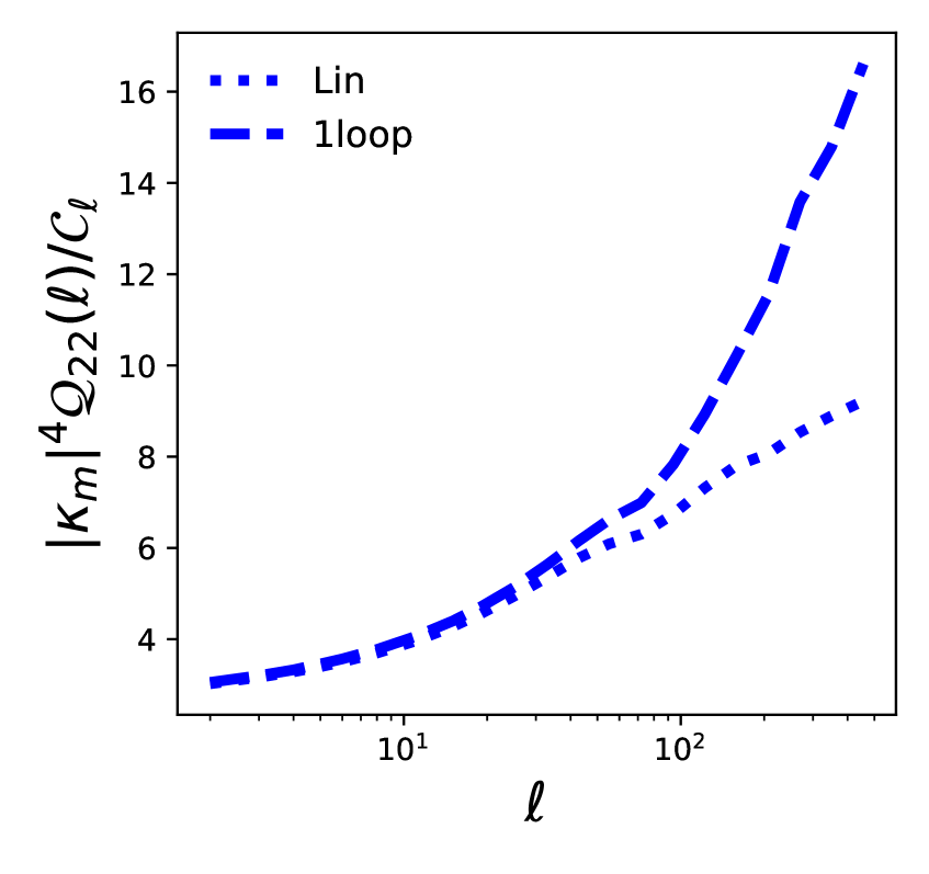
Figure 6: The 3D response functions $|\kappa_{m}|^{\alpha+\beta}Q_{\alpha\beta}$ defined in Eq.(4.9) are shown for the source redshift $z_{s}=1.0$. From left to right panels depict $|\kappa_{m}|^{2}Q_{11}$, $|\kappa_{m}|^{4}Q_{22}$ and $|\kappa_{m}|^{6}Q_{33}$. Various line styles correspond to different analytical models, linear (dashed), one-loop (dotted) as indicated.

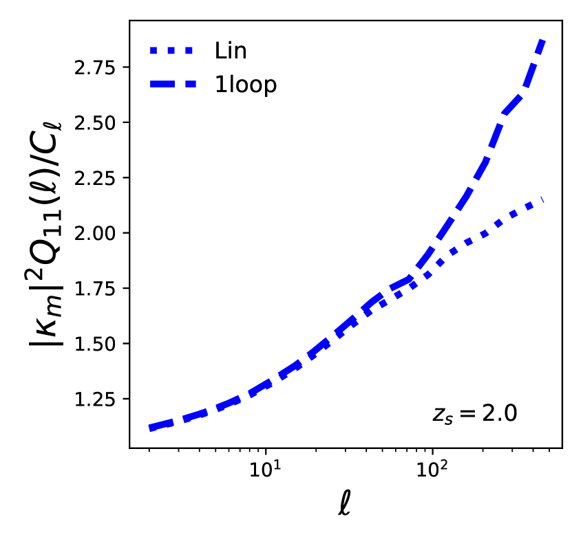
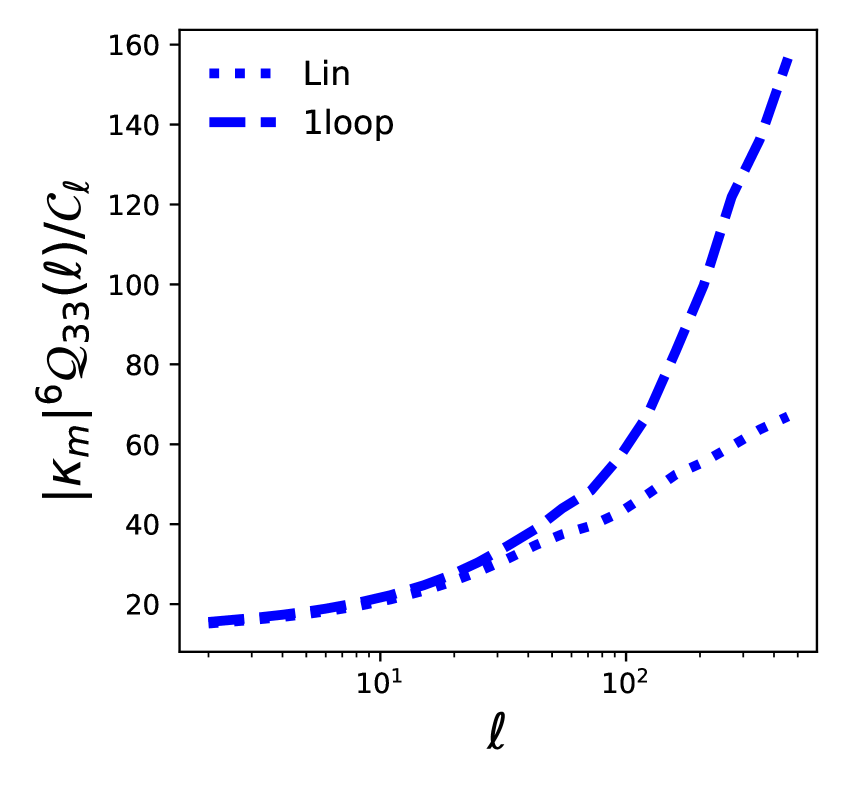
Figure 7: Same as Fig-6 but for $z_{s}=2.0$

.

The local shear power spectrum denoted as ${\cal C}^{\gamma\gamma}_{\ell}(r_{1},r_{2}\big{|}\kappa_{L1},\kappa_{L2})$ is given by:

$${\cal C}^{\gamma\gamma}_{\ell}(r_{1},r_{2}\big{|}\kappa_{L1},\kappa_{L2})={9\Omega^{2}_{M}H_{0}^{4}\over 16\pi^{4}c^{2}}{(\ell+2)!\over(\ell-2)!}\int{dk\over k^{2}}V^{\gamma}_{\ell}(r_{1},k|\delta_{L})V^{\gamma}_{\ell}(r_{2},k|\delta_{L});$$ (4.1a)

$$\kappa_{Li}=\delta_{Li}|\kappa_{mi}|;\quad\kappa_{mi}=-\int_{0}^{r_{si}}drD_{+}(r)\,W_{i}(r).$$ (4.1b)

Here, $\kappa_{mi}$, i.e. the minimum value of $\kappa_{Li}$ depends on the radial distance $r_{i}$ both through the maximum of the integration as well as through the weight ${{\color[rgb]{0,0,0}W_{i}}}$. Notice that the global 3D spectrum ${\cal C}^{\gamma\gamma}_{\ell}(r_{1},r_{2})$ is recovered for $\delta_{L}=0$ in which limit $\kappa_{Li}=0$. The spectroscopic surveys can measure the radial distances with higher accuracy but typically for fewer objects. In comparision photometric surveys target a higher number of galaxies, but in general with larger redshift uncertainities. The formalism here is suitable for photometric surveys. The quantities $V^{\gamma}$ in Eq.(4.1a) is expressed using a new function $U_{\ell}$

$$V^{\gamma}_{\ell}(\eta_{i},k|\delta_{L})\equiv\int\,dz_{p}\,dz^{\prime}n(z_{p})\,p(z^{\prime}|z_{p})W_{i}U_{\ell}(r[z_{p}],k);$$ (4.2a)

$$U_{\ell}(r[z],k|\delta_{L})\equiv{\int_{0}^{r}{dr^{\prime}a^{{\color[rgb]{0,0,0}-1}}(r^{\prime})}{(r-r^{\prime})\over rr^{\prime}}j_{\ell}(kr^{\prime})P^{1/2}(k;r^{\prime}|\delta_{L})}.$$ (4.2b)

Here, $j_{\ell}$ is the spherical Bessel Function of order $\ell$. The cross-power spectrum involving two different redshifts (equivalently, two different radial distances) is often factorized using the corresponding geometric mean, i.e., $P_{\delta}(k,r_{1},r_{2})=[P_{\delta}(k,r_{1})P_{\delta}(k,r_{2})]^{1/2}$. This approximation reduces a higher-dimensional integral to a product of lower-dimensional integrals. The accuracy of this ansatz was scrutinized in [54] in the context of weak lensing and was found to be at the level of $10\%$ for scales $k>5h^{-1}{\rm Mpc}$. However notice that, using Zeld́ovich Approximation ref.[55], it was shown that higher accuracy can be achieved. Indeed, we have a generalised the factorization scheme by adopting it for local power spectrum, i.e., $P_{\delta}(k,r_{1},r_{2}|\delta_{L})=[P_{\delta}(k,r_{1}|\delta_{L})P_{\delta}(k,r_{2}|\delta_{L})]^{1/2}$. Next, by Taylor expanding ${P}^{1/2}_{\delta}(k,t|\delta_{L})$:

$${P}^{1/2}(k,t|\delta_{L})=P^{1/2}(k,t)\sum_{n={{\color[rgb]{0,0,0}0}}}^{\infty}{\delta_{L}^{n}\over n!}T_{n}(k,t).$$ (4.3)

The coefficients $T_{n}$ can be expressed in terms $R_{n}$ using Eq.(4.3).

$$T_{1}={1\over 2}R_{1};$$ (4.4a)

$$T_{2}=-{1\over 2}R_{1}^{2}+R_{2};$$ (4.4b)

$$T_{3}={3\over 8}R_{1}^{3}-{3\over 4}R_{1}R_{2}+{1\over 2}R_{3}.$$ (4.4c)

It is expected that the radius of convergence for the Taylor expansion of $T^{1/2}$ will be smaller than the original Taylor expansion of $T$. We will also Taylor expand the functions ${U}_{\ell}$ and ${V}_{\ell}$:

$${U}_{\ell}(k,t|\delta_{L})=\sum_{n={{\color[rgb]{0,0,0}0}}}^{\infty}{\delta_{L}^{n}\over n!}U^{(n)}_{\ell}(k,t);\quad{V}_{\ell}(k,t|\delta_{L})=\sum_{n={{\color[rgb]{0,0,0}0}}}^{\infty}{\delta_{L}^{n}\over n!}{V}^{(n)}_{\ell}(k,t).$$ (4.5)

This will allow use to express the coefficients $U_{\ell}$ in terms of the response functions $T_{\alpha}$, and subsequently $R_{\alpha}$.

$$U^{(n)}_{\ell}(k,t)={1\over|\kappa_{m}|^{n}}{\int_{0}^{r}{dr^{\prime}a^{{\color[rgb]{0,0,0}-1}}(r^{\prime})}{(r-r^{\prime})\over rr^{\prime}}j_{\ell}(kr^{\prime})T_{n}(k,t)\,P^{1/2}(k;r^{\prime})}.$$ (4.6)

Using the Limber approximation $\lim_{\ell\rightarrow\infty}j_{\ell}(x)=\sqrt{\pi\over 2(\ell+1/2)}\delta_{D}({\ell+1/2}-x)$ we can simplify this to the following form [56]:

$$U^{(n)}_{\ell}(r,k)={1\over|\kappa_{m}|^{n}}{r-{\cal L}(k)\over ka({\cal L}(k))r{\cal L}(k)}\sqrt{\pi\over 2(\ell+1/2)}T^{n}(k,{\cal L}(k))P^{1/2}(k,{\cal L}(k));$$ (4.7)

where we have used the following shorthand notation: ${\cal L}(k)={(\ell+1/2)/k}$. Taylor expanding the power spectrum in a bivariate series we define the response functions for the 3D power spectrum:

$${\cal C}^{\gamma\gamma}_{\ell}(r_{1},r_{2}\big{|}\kappa_{L1},\kappa_{L2})=\sum_{a,b=0}^{\infty}{1\over a!}{1\over b!}\;{\cal Q}_{ab}(r_{1},r_{2},\ell)\;{\kappa^{a}_{L1}}{\kappa^{b}_{L2}}\;{\cal C}^{\gamma\gamma}_{\cal\ell}(r_{1},r_{2}).$$ (4.8)

The 3D response functions ${\cal Q}_{ab}$ of order $ab$ is a function of two source redshifts $r_{1}$ and $r_{2}$ and are given by:

$${\cal Q}_{ab}(r_{1},r_{2},\ell)={9\Omega^{2}_{M}H_{0}^{4}\over 16\pi^{4}c^{2}}{(\ell+2)!\over(\ell-2)!}\int{dk\over k^{2}}G^{a}_{\ell}(r_{1},k)G^{b}_{\ell}(r_{2},k).$$ (4.9)

For the radial distribution of galaxies denoted by $n(z)$ typically the following form is considered:

$$n(z)=(z/z_{e})^{2}\exp[-(z/z_{e})^{3/2}];\quad z_{e}=0.9/\sqrt{2}.$$ (4.10a)

The photometric smoothing is represented by the following Gaussian photometric distribution.

$$p(z|z_{p})={1\over 2\pi\sigma_{z}(z_{p})}\exp\Big{[}-{1\over 2\sigma_{z_{p}}}(z-c_{cal}z_{p}+z_{\rm bias})^{2}\Big{]};$$

$$c_{cal}=1.0;\quad z_{\rm bias}=0.0;\quad\sigma_{z_{p}}=A(1+z_{P});\quad A=0.5.$$ (4.10b)

For the results shown for ${\cal Q}_{ab}$ in Figure-6 and Figure-7, we assume a single source redshift ($z_{s}=1$ or $2$) instead of the source distribution. We also neglect the photo-z error and replaced $p(z|z_{p})$ it with a delta function.

5 $k$-cut Response Functions

As is well known, the cosmic shear statistics is very sensitive to small scale power which depends on poorly understood nonlinear physics as well as baryonic feedback. Many techniques have been developed from brute force N-body simulation to model small scale behaviour with subsequent marginalisation over small scale power spectra to develop emulator based approach that can be combined with fast Monte Carlo Markov Chain schemes. However, each of this techniques are either too expensive or lacks sufficient accuracy required for stage-IV experiments.

A solution to this problem was first proposed in [53] (see also [57]) that is geometric in nature and cuts out the weak lensing spectrum’s sensitivity to small scale structure in a tunable power. We will refer to the power spectra computed in this manner as k-cut power spectra. This method relies on a nulling scheme that is achieved by applying a similarity transform to the weak lensing spectra following [58]. The key aspect of this transformation is that it organises the lensing information in the lens plane instead of the source plane. Next, taking advantage of the fact that each bin constructed in this manner corresponds to a particular lens redshift range, so taking an angular scale cut thus also removes sensitivity to large-k (small scales) in a uniform manner. In this section we generalise the idea idea of k-cut spectra to k-cut response functions [57, 58].

If we consider a set of discrete source planes at radial distances $r_{i}$,

$${\tilde{W}}_{\alpha}(r)=\sum_{i}p^{i}_{\alpha}W_{i}={3\Omega_{M}H_{0}^{2}\over 2c^{2}}a^{-1}(r)\sum_{i;\;r_{i}>r}p^{i}_{\alpha}{d_{A}(r_{i}-r)d_{A}(r)\over d_{A}(r_{i})},$$ (5.1)

where $\{p_{i}\}$ are a set of weights associated with source planes. The key step in implementing the nulling scheme introduced in [58] is to select weights in such a manner that is the weighted convergence $\tilde{\kappa}_{\alpha}$ is only sensitive to lenses in a specific radial distance.

$$\tilde{\kappa}_{\alpha}=\sum_{i}p^{i}_{\alpha}\kappa_{i}.$$ (5.2a)

In the harmonic domain:

$$\tilde{\kappa}_{\alpha,\ell m}=\sum_{i}p^{i}_{\alpha}\kappa_{i,\ell m};$$ (5.2b)

We will refer to above transformation as the Bernardeau-Nishimichi-Taruya (BNT) transformation, and $\tilde{\kappa}_{a}$ as BNT transformed convergence. It can be shown that the BNT weighted power spectra denoted as $\tilde{\cal C}^{\alpha\beta}_{\ell}\equiv\langle\kappa_{\ell m}^{\alpha}\kappa_{\ell m}^{\beta*}\rangle$ is related to the ordinary tomographic spectra ${\cal C}^{ij}_{\ell}\equiv\langle\kappa_{\ell m}^{i}\kappa_{\ell m}^{*j}\rangle$ through the following similarity (BNT) transformation.

$$\tilde{\cal C}^{\alpha\beta}_{\ell}=\sum_{i,j}p^{i}_{\alpha}p^{j}_{\beta}{\cal C}^{ij}_{\ell}.$$ (5.3)

In a more compact matrix notation we can express the similarity transform as:

$$\tilde{\bf C}_{\ell}={\bf M}{\bf C}_{\ell}{\bf M}^{T}.$$ (5.4)

Construction of the transformation matrix ${\bf M}$ from the weights $p^{i}_{\alpha}$, which satisfies various constraints, is detailed in [58, 57]:

$$\tilde{\cal C}^{\alpha\beta}_{\ell}(\tilde{\kappa}_{LX})=\sum_{n=0}^{\infty}{1\over n!}\;\tilde{\cal Q}^{\alpha\beta}_{n}(\ell)\;{\tilde{\kappa}^{n}_{LX}}\tilde{\cal C}^{\alpha\beta}_{\cal\ell}.$$ (5.5)

This is the BNT equivalent of Eq.(2.3). We can now define the position dependent BNT transformed tomographic spectra $\tilde{\cal C}^{\alpha\beta}_{\ell}(\tilde{\kappa}_{LX})$ that depends on $\tilde{\kappa}_{LX}\equiv[\tilde{\kappa}_{L\alpha}\tilde{\kappa}_{L\beta}]^{1/2}$. Going through the algebra we find the equivalent of Eq.(3.11):

$${\tilde{Q}}^{\alpha\beta}_{n}(\ell)={1\over{\cal C}^{\alpha\beta}_{\ell}}{1\over|{\tilde{\kappa}}_{LX}|^{n}}\int_{0}^{r_{s}}d\tilde{r}{{W}^{\alpha}(r){W}^{\beta}(r)\over{d^{2}_{A}}(r)}R_{n}\left[{\ell\over d_{A}(r)},r\right][D_{+}(r)]^{n}P_{\delta}\left({\ell\over d_{A}(r)},r\right).$$ (5.6)

The corresponding expression for tomographic binning is given in Eq.(3.11). Notice the normalisation of the k-cut response function ${\tilde{Q}}^{\alpha\beta}_{\ell}$ is different from that of the ordinary response functions ${Q}^{\alpha\beta}_{\ell}$. The following definitions were used to express $\tilde{\kappa}_{LX}$:

$$\tilde{\kappa}_{\alpha L}=\delta_{L}|\kappa_{\alpha m}|;\quad\quad\tilde{\kappa}_{\alpha m}=\sum_{i}p^{i}_{\alpha}\kappa_{im}(r)=-\int_{0}^{r_{s}}dr\,D_{+}(r)\,\sum_{i}p_{i}w_{i}(r).$$ (5.7a)

Applying a suitable $\ell$ cut-off in Eq.(3.11) we can systematically remove the high-$k$ modes. ‘

6 Results and Discussions

In Figure-1 we show the response functions $Q_{N}$ defined in Eq.(3.11) are shown. From left-to right panels depict $N=1,2$ and $N=3$. The source redshift is at $z_{s}=1$. Various line-styles correspond to different analytical models, linear, one-loop and halo model as indicated. In Figure-2 we present the corresponding results for the source redshift $z_{s}=2.0$. The predictions from one-loop SPT for lower order response functions show relatively higher level of agreement with the HM models

Typically, for the intermediate range of $\ell$ values most models show an increasing trend. While the HM actually shows a declining trend the predictions based on 1-loop saturates at a rather high value. The predictions based on linear theory are relatively more stable. While each of these predictions need to be checked against simulations, the response function technique based on power spectrum that can probe squeezed bispectrum are more easy to implement compared to the detailed modelling of the bispectrum.

In Figure-3 we show the corresponding response functions for the underlying matter distribution $z=1.$ The response functions $R_{N}$ defined in Eq.(3.16b)-Eq.(3.16d) are shown. From left to right panels depict $N=1,2$ and $N=3$. For the response function $R_{1}$ various models agree with each other for $k<h\,Mpc^{-1}$. The disagreement among them is more pronounced at lower $z$ and higher $N$.

In Figure-4 we show the response functions for the correlation function. The source redshift is fixed at $z_{s}=1.$ The response functions $\Sigma_{N}$ defined in Eq.(3.29c) are shown for the source redshift $z_{s}=1.0$. From left to right panels depict $N=1,2$ and $N=3$. Various line styles correspond to different analytical models, linear, one-loop and halo model as indicated. As expected for large separation angle $\theta$ all models show similar trends, but they differ in the small separation regime.

In Figure-5 we have plotted the $T_{N}$ parameters defined in Eq.(4.4a) -  Eq.(4.4c). These coefficients can be obtained by Taylor expanding square roots of the ratio of local and global power spectrum $P^{1/2}(k,r|\delta_{L})/P^{1/2}(k,r)$ and are related to the coefficients $R_{N}$ and are functions of the wave number $k$. The trends in $T_{N}$ with $z$ and $N$ is dictated similar trends in $R_{N}$.

The Figure-6 shows 3D response functions. The 3D response function is defined in Eq.(4.8). In 3D the response function depends on two different source redshiftd $z_{s1}=1$ and $z_{s2}=2$. From left to right panels depict $Q_{11}$, $Q_{22}$ and $Q_{33}$. We show these results for linear theory and 1-loop SPT. In agreement with their projected counterparts one-loop corrections show departure at increasing lower $\ell$.

7 Conclusion and Future Prospects

Several authors in recent years have used SU formalism in the context of galaxy clustering studies (e.g. [60, 59, 61]). In this paper we have introduced the response functions approach for analysing the higher-order statistics of weak lensing convergence maps. We have also extended the real space based correlation function results [62] developed for galaxy surveys for the case of weak lensing surveys. The response functions for the correlation functions presented here can be generalised to $3\times 2$ correlation functions typically used to analyse the data weak lensing surveys. For a different approach to response function see [32].

We have explored the response functions for weak lensing power spectrum. However, the formalism discussed here can be generalised for bispectrum and other higher-order statistics. Separate Universe N-body simulations for dark matter clustering are currently available, but separate universe weak lensing convergence or shear maps from such simulations are currently unavailable. We hope our study will motivate development of such simulations. The validity range of various approximations used in our derivation can then be tested when such simulations become available.

The forward modelling studies based on power spectrum have gained popularity in recent years. These studies can be extended to include the information regarding non-Gaussianity using the response functions introduced here without much additional computational overhead.

To compute the signal-to-noise associated with the response functions we have studied here, the covariance matrices for these statistics is needed, which will be presented in a separate publication.

The preferential alignments of halos due to tidal interactions is responsible for what is also known as intrinsic alignment (IA) and is considered to be a systematics for weak lensing surveys see [63] for KiDS and [64] for DES. It is believed that for analysing the future surveys such as Euclid and LSST it will be vital to understand IA in a lot more detail. Many authors on the other hand have gone a step forward and underlined the usefulness of IA as a cosmological probe. Most statistical modelings of IA is devoted to halo model based approaches. In [44] an effective field theory (EFT) based approach was developed for modelling of power spectrum and in [65] the authors have focused on bispectrum induced by IA. A response function based approach that only relies on modelling of power spectrum and its derivatives will be presented elsewhere.

The theoretical framework developed here will also be useful beyond weak lensing studies in other areas of cosmology, e.g., in the context of Lyman-$\alpha$ [66] absorption studies, 21cm studies [67] and studies of CMB secondaries[69].

Appendix A Perturbative Results

Following [70], the expression for the exact 2D expression is given by:

$$S_{3}(\ell)=N_{2}\left[{24\over 7}-{1\over 2}(n+1)\right]$$ (A.1a)

$$N_{2}={\int_{0}^{r_{s}}}dr{\omega^{3}(r)\over d^{4+2n}_{A}(r)}\Big{/}\left({\int_{0}^{r_{s}}}dr{\omega(r)\over d^{4+2n}_{A}(r)}\right)^{2}$$ (A.1b)

and also the doubly squeezed trispectrum is given by:

$$S_{3}(\ell)=N_{3}\left[{1473\over 79}-{195\over 14}(n+2)+{3\over 4}(n+2)^{2}\right]$$ (A.2a)

$$N_{3}={\int_{0}^{r_{s}}}dr{\omega^{4}(r)\over d^{6+3n}_{A}(r)}\Big{/}\left({\int_{0}^{r_{s}}}dr{\omega^{2}(r)\over d^{6+3n}_{A}(r)}\right)^{2}$$ (A.2b)

References

• [1] Weak Gravitational Lensing, M. Bartelmann, P. Schneider, 2001, Phys. Rep., 340, 291, [arxiv/9912508]
• [2] Cosmology with Weak Lensing Surveys, D. Munshi, P. Valageas, L. Van Waerbeke, A. Heavens, 2008, Phys.Rept., 462, 67, [arxiv/0612667]
• [3] The Hyper Suprime-Cam SSP Survey: Overview and Survey Design, Aihara H. et al., 2018, Publications of the Astronomical Society of Japan, Volume 70, Issue SP1, S4, [arXiv/1704.05858]
• [4] Cosmology from Cosmic Shear with DES Science Verification Data, The Dark Energy Survey Collaboration, T Abbott, F. B. Abdalla, S. Allam, et al., 2016, PRD, 94, 022001, [arxiv/1507.0552]
• [5] Gravitational Lensing Analysis of the Kilo Degree Survey, K. Kuijken, C. Heymans, H. Hildebrandt, et al., 2015, MNRAS, 454, 3500, [astro-ph/1507.00738]
• [6] Euclid Definition Study Report, R. Laureijs, J. Amiaux, S. Arduini, et al. 2011, ESA/SRE(2011)12.
• [7] LSST: a complementary probe of dark energy, J. A. Tyson, D. M. Wittman, J. F. Hennawi, D. N Spergel, 2003, Nuclear Physics B Proceedings Supplements, 124, 21, [astro-ph/0209632]
• [8] National Research Council. 2010. New Worlds, New Horizons in A&A. The National Academies Press.
• [9] Beyond the Cosmological Standard Model,, A. Joyce, B. Jain, J. Khoury, M. Trodden, 2015, Phys. Rep., 568, 1, [astro-ph/1407.0059]
• [10] Modified Gravity and Cosmology, T. Clifton, P. G. Ferreira, A. Padilla, S. Skordis, 2012, Phys. Rep., 513, 1, 1, [astro-ph/1106.2476]
• [11] Massive neutrinos and cosmology, J. Lesgourgues, S. Pastor, 2006, Phys. Rep., 429, 307, [astro-ph/1610.02956]
• [12] Large scale structure of the universe and cosmological perturbation theory, F. Bernardeau, S. Colombi, E. Gaztanaga, R. Scoccimarro, 2002, Phys.Rep. 367, 1, [astro-ph/0112551]
• [13] The three-point correlation function of cosmic shear: I. The natural components P. Schneider, M. Lombardi, 2003, A&A, 397, 809 [arXiv/0207454]
• [14] The three-point correlation function of cosmic shear. II: Relation to the bispectrum of the projected mass density and generalized third-order aperture measures P. Schneider, M. Kilbinger, M. Lombardi, 2005, A&A, 431, 9, [astro-ph/0308328]
• [15] The Three-Point Correlation Function for Spin-2 Fields M. Takada, B. Jain, 2003, ApJ, 583, L49 [arXiv/0210261]
• [16] Cosmological parameters from weak lensing power spectrum and bispectrum tomography: including the non-Gaussian errors I. Kayo, M. Takada [arXiv/1306.4684]
• [17] Weak lensing from space: first cosmological constraints from three-point shear statistics E. Semboloni, T. Schrabback, L. van Waerbeke, S. Vafaei, J. Hartlap, S. Hilbert, 2010, MNRAS, 410, 143 [arXiv/1005.4941]
• [18] Non-Gaussianity from Inflation: Theory and Observations N. Bartolo, E. Komatsu, S. Matarrese, A. Riotto 2004, Phys.Rept. 402, 103 [astro-ph/0406398]
• [19] Higher order statistics of shear field: a machine learning approach, C. Parroni, E. Tollet, V. F. Cardone, R. Maoli, R. Scaramella, [astro-ph/1612.02264]
• [20] Weak lensing shear and aperture-mass from linear to non-linear scales D. Munshi, P. Valageas, A. J. Barber MNRAS, 2004, 350, 77 [astro-ph/1612.02264]
• [21] Cylinders out of a top hat: counts-in-cells for projected densities C. Uhlemann, 2018, MNRAS, 477, 2772U, [arXiv/1711.04767]
• [22] Cosmological constraints with weak lensing peak counts and second-order statistics in a large-field survey, A. Peel, C.-A. Lin, F. Lanusse, A. Leonard, J.-L. Starck, M. Kilbinger, 2017, A&A 599, A79, [arXiv/1612.02264]
• [23] Weak Lensing Skew-Spectrum, D. Munshi, T. Namikawa, T. D. Kitching, J. D. McEwen, F. R. Bouchet, 2020, MNRAS, 498, 6057, [arXiv/2006.12832]
• [24] Estimating the Integrated Bispectrum from Weak Lensing Maps, D. Munshi, J. D. McEwen, T. Kitching, P. Fosalba, R. Teyssier, J. Stade,l 2020, MNRAS, 493, 3985, [arXiv/1902.04877]
• [25] New Optimised Estimators for the Primordial Trispectrum, D. Munshi, A. Heavens, A. Cooray, J. Smidt, P. Coles, P. Serra, 2011, MNRAS, 412, 1993, arXiv/0910.3693
• [26] Morphology of Weak Lensing Convergence Maps D. Munshi, T. Namikawa, J. D. McEwen, T. D. Kitching, F. R. Bouchet, [arXiv/2010.05669]
• [27] Matter trispectrum: theoretical modelling and comparison to N-body simulations D. Gualdi, S. Novell, H. Gil-MarΓ­n, L. Verde 2021, JCAP, 01, 015 arXiv/2009.02290,
• [28] Persistent homology in cosmic shear: constraining parameters with topological data analysis S. Heydenreich, B. BrΓΌck, J. Harnois-DΓ©raps 2021, A&A, 648, 74 arxiv/2007.13724,
• [29] Exact Extreme Value Statistics and the Halo Mass Function I. Harrison, P. Coles MNRAS 418, L20-L24 (2011) arXiv/1108.1358,
• [30] The position-dependent matter density probability distribution function D. Jamieson, M. Loverde 2020, PRD 102, 123546 arxiv/2010.07235,
• [31] An adapted filter function for density split statistics in weak lensing P. Burger, P. Schneider, V. Demchenko, J. Harnois-Deraps, C. Heymans, H. Hildebrandt, S. Unruh 2020, A&A 642, A161 (see also arXiv/2006.10778).
• [32] Response function of the large-scale structure of the universe, to the small scale inhomogeneities, T. Nishimichi, F. Bernardeau, A. Taruya, Physics Letters B, 762, 247, arXiv/1411.2970
• [33] The Weak Lensing Bispectrum Induced By Gravity, D. Munshi, T. Namikawa, T. D. Kitching, J. D. McEwen, R. Takahashi, F. R. Bouchet, A. Taruya, B. Bose, 2020, MNRAS, 493, 3985 arXiv/1910.04627
• [34] Phase Correlations in Non-Gaussian Fields T. Matsubara, 2003, ApJ., 591, L79 [astro-ph/0303278]
• [35] Statistics of Fourier Modes in Non-Gaussian Fields T. Matsubara, 2007, ApJS, 170, 1, [astro-ph/0610536]
• [36] A New Estimator for Phase Statistics D. Munshi, R. Takahashi, J. D. McEwen, T. D. Kitching, F. R. Bouchet, 2022, JCAP, 05, 006, [arXiv/2109.08047]
• [37] Higher-order statistics of shear field: a machine learning approach, C. Parroni, E. Tollet, V. F. Cardone, R. Maoli, R. Scaramella 2021, A&A 645, 123 [arXiv/2011.10438xs]
• [38] Position-dependent power spectrum: a new observable in the large-scale structure C.-T. Chiang [arXiv/1508.03257]
• [39] Planck 2015 results. XIII. Cosmological parameters Planck Collaboration, 2016, A&A, 594, A13
• [40] Galaxy bias and non-linear structure formation in general relativity T. Baldauf, U. Seljak, L. Senatore, M. Zaldarriaga, 2011, JCAP, 10, 031
• [41] Power spectrum super-sample covariance M. Takada, W. Hu, 2013, PRD, 87, 123504
• [42] Efficient Evaluation of Cosmological Angular Statistics V. Assassi, M. SimonoviΔ‡, M. Zaldarriaga, 2017, JCAP, 11, 054, [arXiv/1705.05022]
• [43] Halo Models of Large Scale Structure A. Cooray, R. Sheth 2002, Phys.Rept., 372, 1 [astro-ph/0206508]
• [44] Precision Comparison of the Power Spectrum in the EFTofLSS with Simulations S. Foreman, H. Perrier, L. Senatore 2016, JCAP, 05, 027 [arXiv/1507.05326]
• [45] Accurate cosmic shear errors: do we need ensembles of simulations? A. Barreira, E. Krause, F. Schmidt 2018, JCAP, 10, 053 [arXiv/1807.04266]
• [46] Covariances for cosmic shear and galaxy-galaxy lensing in the response approach R. Takahashi, T. Nishimichi, M. Takada, M. Shirasaki, K. Shiroyama 2019, MNRAS, 482, 4253 [arXiv/1805.11629]
• [47] Position-Dependent Correlation Function of Weak Lensing Convergence D. Munshi, G. Jung, T. D. Kitching, J. McEwen, M. Liguori, T. Namikawa, A. Heavens [arXiv/2104.01185]
• [48] Position-dependent correlation function from the SDSS-III Baryon Oscillation Spectroscopic Survey Data Release 10 CMASS Sample C.-T. Chiang, C. Wagner, A. G. SΓ‘nchez, F. Schmidt, E. Komatsu 2015, JCAP, 09, 028 [arXiv/1504.03322]
• [49] Response approach to the integrated shear 3-point correlation function: the impact of baryonic effects on small scales A. Halder, A. Barreira [arXiv/2201.05607]
• [50] The integrated 3-point correlation function of cosmic shear A. Halder, O. Friedrich, S. Seitz, T. N. Varga 2021, MNRAS, 506, 2780 [arXiv/2201.05607]
• [51] 3D weak lensing A. F. Heavens, 2003, MNRAS, 343, 1327 [arXiv/0304151]
• [52] Weak lensing analysis in three dimensions P. G. Castro, A. F. Heavens, T. D. Kitching 2005, PRD, 72, 023516 [astro-ph/0503479]
• [53] 3D Photometric Cosmic Shear T. D. Kitching, A. F. Heavens, L. Miller 2011, MNRAS, 413, 2923 [arXiv/1007.2953]
• [54] Unequal-Time Correlators for Cosmology T. D. Kitching, A. F. Heavens 2017, PRD, 95, 063522 [arXiv/1612.00770]
• [55] Unequal time correlators and the Zeldovich approximation N. E. Chisari, A. Pontzen 2019, PRD 100, 023543 [arXiv/1905.02078]
• [56] Accurate photometric redshifts for the CFHT Legacy Survey calibrated using the VIMOS VLT Deep Survey O. Ilbert, A&A 2006, 457, 841 [astro-ph/0603217]
• [57] k-cut Cosmic Shear: Tunable Power Spectrum Sensitivity to Test Gravity P. L. Taylor, F. Bernardeau, T. D. Kitching 2018, PRD, 98, 083514 [arxiv/1809.03515]
• [58] Cosmic shear full nulling: sorting out dynamics, geometry and systematics, F. Bernardeau, T. Nishimichi, A. Taruya, 2014, MNRAS, 445, 1526, [arXiv/1312.0430]
• [59] The angle-averaged squeezed limit of nonlinear matter N-point functions, C. Wagner, F. Schmidt, C.-T. Chiang, E. Komatsu, 2015, JCAP, 08, 042 [arxiv/1503.03487]
• [60] Position-dependent power spectrum of the large-scale structure: a novel method to measure the squeezed-limit bispectrum, C.-T. Chiang, C. Wagner, F. Schmidt, E. Komatsu, 2014, JCAP, 05, 048 [arxiv/1106.5507]
• [61] Separate universe approach to evaluate nonlinear matter power spectrum for non-flat $\Lambda$CDM model R. Terasawa, R. Takahashi, T. Nishimichi, M. Takada, 2022, submitted to PRD, [arxiv/2205.10339]
• [62] Position-dependent correlation function from the SDSS-III Baryon Oscillation Spectroscopic Survey Data Release 10 CMASS Sample, C.-T. Chiang, C. Wagner, A. G. SΓ‘nchez, F. Schmidt, E. Komatsu, 2015. JCAP, 09, 028, [arXiv/1504.03322]
• [63] KiDS-1000 Methodology: Modelling and inference for joint weak gravitational lensing and spectroscopic galaxy clustering analysis, B. Joachimi, et al., 2021, A&A, 646, A129 [arXiv/1701.03375]
• [64] Dark Energy Survey Year 3 Results: Three-Point Shear Correlations and Mass Aperture Moments, L. F. Secco, et al., 2022, PRD, 105, 023515, [arXiv/2201.05227]
• [65] Three-point intrinsic alignments of dark matter halos in the IllustrisTNG simulation, S. Pyne, A. Tenneti, B. Joachimi, [arXiv/2204.10342]
• [66] Response approach to the squeezed-limit bispectrum: application to the correlation of quasar and Lyman-$\alpha$ forest power spectrum, C-T Chiang, A. M. Cieplak, F. Schmidt, A. Slosar, 2017, JCAP 06, 0220, [arXiv/1701.03375]
• [67] The large-scale 21-cm power spectrum from reionization, I. Georgiev, G. Mellema, S. K. Giri, R. Mondal, [arXiv/2110.13190]
• [68] An EFT description of galaxy intrinsic alignments, Z. Vlah, C. N. Elisia, F. Schmidt, 2020, JCAP, 01, 025, [arXiv/1910.08085]
• [69] Extracting the late-time kinetic Sunyaev-Zel’dovich effect, D. Munshi, I. T. Iliev, K. L. Dixon, P. Coles, 2016, MNRAS, 463, 2425, [arXiv/1511.03449]
• [70] The Integrated Bispectrum and Beyond D. Munshi, P. Coles 2017, JCAP, 02, 010 [arXiv/1608.04345]