Cost-efficient Payoffs under Model Ambiguity

Abstract

Dybvig (1988a, b) solves in a complete market setting the problem of finding a payoff that is cheapest possible in reaching a given target distribution (“cost-efficient payoff”). In the presence of ambiguity, the distribution of a payoff is, however, no longer known with certainty. We study the problem of finding the cheapest possible payoff whose worst-case distribution stochastically dominates a given target distribution (“robust cost-efficient payoff”) and determine solutions under certain conditions. We study the link between “robust cost-efficiency” and the maxmin expected utility setting of Gilboa and Schmeidler, as well as more generally with robust preferences in a possibly non-expected utility setting. Specifically, we show that solutions to maxmin robust expected utility are necessarily robust cost-efficient. We illustrate our study with examples involving uncertainty both on the drift and on the volatility of the risky asset.

KEYWORDS: Cost-efficient payoffs, model ambiguity, maxmin utility, robust preferences, drift and volatility uncertainty
JEL classification: C02, C63, D80
AMS classification: 91B30, 62E17

1 Introduction

In a (complete) market without ambiguity, Dybvig (1988a, b) characterizes optimal payoffs for agents having law-invariant increasing preferences (e.g., expected utility maximizers). His result is based on the observation that any optimal payoff $X$ must be cost-efficient in the sense that there cannot exist another payoff with the same probability distribution that is strictly cheaper than $X$. He then derives, for a given target distribution of terminal wealth, the payoff that achieves this target distribution at the lowest possible cost (cost-efficient payoff). Optimal portfolios are thus driven by distributional constraints rather than appearing as a solution to some optimal expected utility problem. In this regard, Brennan and Solanki (1981) note that “from a practical point of view it may well prove easier for the investor to choose directly his optimal payoff function than it would be for him to communicate his utility function to a portfolio manager.” Sharpe et al. (2000) and Goldstein et al. (2008) introduce a tool called the distribution builder, which makes it possible for investors to analyze distributions of terminal wealth and to choose their preferred one among alternatives with equal cost; see also Sharpe (2011) and Monin (2014). Moreover, Goldstein et al. (2008) argue that such a tool makes it possible to better elicit investor’s preferences.

Our main objective is to extend Dybvig’s results when there is uncertainty on the real-world probability measure. Uncertainty has become a prime issue in many academic domains, from economics to environmental science and psychology. Model ambiguity refers to random phenomena or outcomes whose probabilities are themselves unknown. For instance, the random outcome of a coin toss is subject to model uncertainty when the probability of the coin showing either a head or a tail is not or is at most partially known. This notion of model ambiguity goes back to Knight (1921) and is therefore commonly referred to as Knightian uncertainty.

In the presence of ambiguity, the probability distribution of a payoff is not anymore determined. Thus, looking for a minimum cost payoff with a given probability distribution is no longer possible. However, investors may still determine a desired distribution function that they would like to achieve “at least”. In this paper, we look for a minimum cost payoff that dominates a target distribution for a chosen stochastic integral order under any plausible real-world probability distribution. Our contributions are three-fold. First, we solve this problem explicitly for a general stochastic ordering under certain assumptions. Solutions to this problem are called “robust cost-efficient.” Second, we draw connections between such a minimum cost payoff and the problem of finding an optimal portfolio under ambiguity for general sets of robust preferences. Third, we present a number of examples, including one on the robust portfolio choice in the presence of volatility uncertainty.

Our results generalize the results on cost-efficiency given in Dybvig (1988a, b), Cox and Leland (2000) and Bernard et al. (2014, 2015). When there is no ambiguity on the real-world probability, the robust cost efficient payoffs coincide with the cost-efficient payoffs studied in the literature. To derive our results, we build on the so-called quantile approach to solve the optimization of a law invariant increasing functional, e.g., Schied (2004), Carlier and Dana (2006, 2008, 2011), Jin and Zhou (2008), He and Zhou (2011a, b), Bernard et al. (2014), Xu (2016) and Rüschendorf and Vanduffel (2020).

Specifically, we consider a static setting but we have incomplete markets and are thus able to address uncertainty about volatility. We show that, under certain conditions, the solution to a general robust portfolio maximization problem is equal to the solution of a classical portfolio maximization problem under a least favorable measure $\mathbb{P}^{\ast}$ with respect to some stochastic ordering. This was already shown by Schied (2005) for the case of robust expected utility theory and using first order stochastic dominance ordering; here, however, we show that these results extend to the case of more general preferences. Specifically, we focus on the case of first order and second order stochastic dominance.

Furthermore, we show that there is a natural correspondence between optimal portfolios in the maxmin utility setting of Gilboa and Schmeidler (1989), with a concave increasing utility, and robust cost-efficient payoffs: for any robust cost-efficient payoff $X^{\ast}$, there is a utility function such that $X^{\ast}$ solves the maxmin expected utility maximization problem. We further show that the solution to a robust maximization problem with respect to a general family of preferences is cost-efficient. This result implies that instead of solving a robust maximization problem with respect to a general family of preferences one could solve an expected utility maximization problem under the single measure $\mathbb{P}^{\ast}$ for a suitable concave utility function.

The literature on optimal payoff choice under ambiguity includes the seminal setting of Gilboa and Schmeidler (1989) that is, the so-called “maxmin expected utility,” which was later referred to as robust utility functional by Schied et al. (2009). Specifically, these authors characterize preferences that have a robust utility numerical representation $\underset{\mathbb{P}\in\mathcal{P}}{\min}\,E_{\mathbb{P}}[u(X)]$ for some set of probabilities $\mathcal{P}$. Gundel (2005) provides a dual characterization of the solution for robust utility maximization in both a complete and an incomplete market model. Klibanoff et al. (2005) distinguish between subjective beliefs, e.g., the definition of the set of possible or plausible subjective probability measures, and ambiguity attitude, i.e., a characterization of the agent’s behavior toward ambiguity. Based on Klibanoff et al. (2005), Gollier (2011) analyzes the effect of ambiguity aversion on the demand for the uncertain asset in a portfolio choice problem.

Schied (2005) solves the maximization problem of maxmin expected utility of Gilboa and Schmeidler (1989) in a general complete market model with dynamic trading, provided there is a least favorable measure with respect to FSD ordering. Specifically, he finds that the optimum for the maxmin utility setting of Gilboa and Schmeidler (1989) can be derived in the standard expected utility setting under the least favorable measure. Schied (2005) works with a complete market model and mainly in a static setting; dynamics only come into play when the martingale method is applied to the static solutions. A survey on robust preferences and robust portfolio choice can be found in Schied et al. (2009).

The paper is organized as follows. The robust cost-efficiency problem is described in Section 2. In Section 3, we solve the robust cost-efficiency problem, and we include two examples in a log-normal market with uncertainty on the drift and the volatility along with another example in a Lévy market in which the physical measure is obtained by the Esscher transform. In Section 4, we develop the correspondence between robust cost-efficient payoffs and strategies that solve a robust optimal portfolio problem, including the maxmin utility setting of Gilboa and Schmeidler (1989) as a special case. In Section 5, we show that the solution to a general robust optimal portfolio problem can also be obtained as a solution to the maximization of the maxmin utility setting of Gilboa and Schmeidler (1989) for a well-chosen concave utility function. Section 6 concludes.

2 Problem statement

We assume a static market setting in which trading only takes place today and at the end of the planning horizon $T>0$. There is a bank account earning the continuously compounded risk-free interest rate $r\in\mathbb{R}$. Let $\mathbb{R}_{+}=[0,\infty)$. Let $S_{T}:\Omega\rightarrow\mathbb{R}_{+}$ represent the random value of a risky asset at maturity. We denote by $S_{0}>0$ its current value and by $\mathcal{F}$ the $\sigma$-algebra $S_{T}$ generates. Let $\mathcal{P}$ be a set of equivalent real-world probability measures on $(\Omega,\mathcal{F})$. The set $\mathcal{P}$ can be thought of as a collection of probability measures that the investor deems plausible for the market. We define the set of payoffs $\mathcal{X}=\left\{g(S_{T}),\,g:\mathbb{R}_{+}\to\mathbb{R}_{+}\text{ is measurable and }E_{\mathbb{Q}}[|g(S_{T})|]<\infty\right\},$ where $\mathbb{Q}$ is a martingale measure, equivalent to all $\mathbb{P}\in\mathcal{P}.$ Furthermore, for any $X\in\mathcal{X}$, its price is given by $e^{-rT}E_{\mathbb{Q}}[X]$.

Remark 2.1.

Under the assumption that all call options $(S_{T}-K)^{+}$, $K\geqslant 0$ are traded and under the condition that the function mapping every $K\geqslant 0$ to the price of $(S_{T}-K)^{+}$ is twice differentiable with respect to $K$, Breeden and Litzenberger (1978) show that any $X\in\mathcal{X}$ can almost surely be replicated using a static portfolio of calls.

Consider an investor with a finite budget and planning horizon $T>0$ who wishes to invest in the market whilst having ambiguous views on the real-world probability measure. How can she find her optimal investment strategy? As in Schied (2005), she could maximize some robust expected utility à la Gilboa and Schmeidler (1989). The basic idea is then to look for a payoff that maximizes the worst case expected utility, reflecting the idea that the investor aims to protect against the worst whilst hoping for the best. However, it seems easier for investors to specify the desired probability distribution of the terminal wealth rather than a utility function (Brennan and Solanki (1981), Sharpe et al. (2000), Goldstein et al. (2008)).

As in Dybvig (1988), Sharpe et al. (2000), Vrecko and Langer (2013), and Bernard et al. (2014), we thus assume in this paper that the investor specifies a desired (cumulative) distribution function $F_{0}$ of future terminal wealth. Once the investor understands which distribution function $F_{0}$ is acceptable to her, the natural question arises as to how to find, under ambiguity, the cheapest portfolio with a distribution function at maturity that is “at least as good” as $F_{0}$. This is the robust cost-efficiency problem formalized hereafter. In this regard, we need to recall the concept of integral stochastic ordering, see e.g., Denuit et al. (2005). In this paper, we denote by $\mathbb{F}$ a set of measurable functions from $\mathbb{R}_{+}$ to $\mathbb{R}$.

Definition 2.2 (Stochastic integral ordering).

Let $G$ and $F$ be two distribution functions with support on $\mathbb{R_{+}}$. The distribution function $G$ dominates the distribution function $F$ in integral stochastic ordering with respect to the set $\mathbb{F}$, in notation $F\preceq_{\mathbb{F}}G$, if

$$\forall f\in\mathbb{F},\quad\int_{\mathbb{R_{+}}}f(x)dF\leqslant\int_{\mathbb{R_{+}}}f(x)dG,$$

such that expectations are finite.

Let $\mathbb{F}_{FSD}$ denote the set of all non-decreasing functions from $\mathbb{R}_{+}$ to $\mathbb{R}$. The corresponding stochastic integral ordering is called first order stochastic dominance (FSD). Furthermore, let $\mathbb{F}_{SSD}$ denote the set of all non-decreasing and concave functions from $\mathbb{R}_{+}$ to $\mathbb{R}$. The corresponding stochastic integral ordering is called second order stochastic dominance (SSD). It is well-known that FSD reflects the common agreement of all investors with law-invariant increasing preferences (Bernard et al., 2015, Theorem 1), whereas SSD order reflects the common agreement of those who have law-invariant increasing and diversification loving preferences (risk averse investors) (Bernard and Sturm, 2023, Corollary 2.6).

Problem 1 (Robust cost-efficiency problem).

The $\mathbb{F}-$robust cost-efficiency problem for a distribution function $F_{0}$ is defined as

$$\underset{X\in\mathcal{B}_{F_{0}}^{\mathbb{F}}}{\inf}e^{-rT}E_{\mathbb{Q}}[X],$$ (2.1)

in which $\mathcal{B}_{F_{0}}^{\mathbb{F}}$ denotes a class of admissible payoffs defined as

$$\mathcal{B}_{F_{0}}^{\mathbb{F}}=\left\{X\in\mathcal{X}\,:\,\forall\mathbb{P}\in\mathcal{P}:\,F_{0}\preceq_{\mathbb{F}}F_{X}^{\mathbb{P}}\right\}.$$

A solution to (2.1) is called a $\mathbb{F}-$robust cost-efficient payoff.

As discussed above, the target distribution function of the investor is $F_{0}$. That is, we are interested in all payoffs that have a distribution function at maturity that is at least as good as $F_{0}$ under all plausible scenarios $\mathbb{P\in\mathcal{P}}$. For example, when $\mathbb{F}=\mathbb{F}_{FSD}$, we care about payoffs having distribution functions $F_{X}^{\mathbb{P}},$ $\mathbb{P}\in\mathcal{P}$ that dominate $F_{0}$ in FSD. In order not to “throw away investors’ money”, see Dybvig (1988), we then aim to determine the cheapest payoff among the payoffs in the admissible set $\mathcal{B}_{F_{0}}^{\mathbb{F}}$. In Theorem 3.1 we provide solutions to the $\mathbb{F}-$robust cost-efficiency problem (2.1) under regularity conditions on the set $\mathbb{F}$ and $F_{0}$.

Dybvig (1988a, b) introduced the standard cost-efficiency problem without ambiguity on the set of physical measures; that is, when $\mathcal{P}=\{\mathbb{P}\}$. Specifically, for some fixed $\mathbb{P}\in\mathcal{P}$, the problem he considered reads as

$$\underset{X\in\mathcal{A}_{F_{0}}^{\mathbb{P}}}{\inf}e^{-rT}E_{\mathbb{Q}}[X],$$ (2.2)

where

$$\mathcal{A}_{F_{0}}^{\mathbb{P}}=\left\{X\in\mathcal{X}\,:\,F_{0}=F_{X}^{\mathbb{P}}\right\}.$$

We refer to this problem as the standard cost-efficiency problem. Furthermore, we say that a payoff $X$ that is distributed with $F_{X}^{\mathbb{P}}$ is $\mathbb{P}-$cost-efficient if $X$ solves the standard cost-efficiency problem (2.2) under $\mathbb{P}$ w.r.t. $F_{0}=F_{X}^{\mathbb{P}}$. By Bernard et al. (2014), a payoff $X$ is $\mathbb{P}-$cost-efficient if and only if $X$ is non-increasing in the state price $\mathbb{P}-$a.s., see also Schied (2004, Proposition 2.5).

The standard cost-efficiency problem (2.2) has been solved in Dybvig (1988a, b) and in Bernard et al. (2014), see also Lemma B.1 in the Appendix. In Corollary 3.5 we show that in the case in which $\mathcal{P}$ is a singleton, the solution to the $\mathbb{F}-$robust cost-efficiency problem is unique and coincides with the solution to the standard cost-efficiency problem.

Remark 2.3.

For a fixed $X\in\mathcal{X}$, we have that in general $F_{X}^{\mathbb{P}}$ cannot be equal to $F_{0}$ for all $\mathbb{P}\in\mathcal{P}$. Therefore, we replace the condition $F_{0}=F_{X}^{\mathbb{P}}$ in the standard cost-efficiency problem with $F_{0}\preceq_{\mathbb{F}}F_{X}^{\mathbb{P}}$ in the robust setting.

The next example anticipates Sections 3.1.1 and 3.1.2 and is designed to help distinguish between the standard and the robust cost-efficiency problem.

Example 2.4.

(Cost-efficient payoffs). Assume the real-world distribution function of $S_{T}$ is log-normal. There are three investors: one investor assumes that the drift of $S_{T}$ under the physical measure, denoted by $\mathbb{P}^{\mu_{1}}$, is equal to $\mu_{1}>r$. Another investor assumes that the drift is given by $\mu_{2}>\mu_{1}$ under the physical measure, denoted by $\mathbb{P}^{\mu_{2}}$. A third investor has ambiguity and assumes that the drift lies in the interval $[\mu_{1},\mu_{2}]$, and thus considers a set $\mathcal{P}=\{\mathbb{P}^{\mu},\,\mu\in[\mu_{1},\mu_{2}]\}$ as the set of all plausible probability measures on $(\Omega,\mathcal{F})$. The cheapest payoffs to obtain a fixed target distribution function $F_{0}$ are well-known for investor one and two and are given by

$$X_{1}^{\ast}:=F_{0}^{-1}\left(F_{S_{T}}^{\mathbb{P}^{\mu_{1}}}(S_{T})\right)\quad\text{and}\quad X_{2}^{\ast}:=F_{0}^{-1}\left(F_{S_{T}}^{\mathbb{P}^{\mu_{2}}}(S_{T})\right),$$

respectively; see Proposition 3 in Bernard et al. (2014). Within the set $\mathcal{P}$, $\mathbb{P}^{\mu_{1}}$ corresponds to a pessimistic view of the stock price behavior, and we will see in Section 3.1.1 that $X_{1}^{\ast}$ also solves the robust cost-efficiency problem for $F_{0}$ if $\mathbb{F}=\mathbb{F}_{FSD}$. In the case in which $\mathbb{F}=\mathbb{F}_{SSD}$, $X_{1}^{\ast}$ also solves the robust cost-efficiency problem if additionally $F_{0}^{-1}\circ F_{S_{T}}^{\mathbb{P}^{\mu_{1}}}$ is concave; see Section 3.1.2. This example illustrates that the solution to the standard cost-efficiency problem for arbitrarily $\mathbb{P}\in\mathcal{P}$ and the solution to the robust cost-efficiency problem generally do not coincide.

Remark 2.5 (Uncertainty on target distribution $F_{0}$).

As in Rüschendorf and Wolf (2016), we could also consider uncertainty on the target distribution function $F_{0}.$ Specifically, in Rüschendorf and Wolf (2016) it is assumed that the investor specifies finitely many acceptable distribution functions $F^{1}_{0},...,F^{N}_{0}$. As all $N$ distribution functions are acceptable to the investor, she could solve the robust cost-efficiency problem $N$ times and buy the cheapest solution among the $N$ solutions. It is also possible to consider a continuum of acceptable distribution functions: generalizing Rüschendorf and Wolf (2016) slightly, we could consider the set

$$\mathcal{G}=\left\{F\ |F\ \text{is a cdf},\quad F_{0}\preceq_{\mathbb{F}}F\right\},$$

as the set of distribution functions that are acceptable to the investor or client. We could then consider the cost-efficiency problem with uncertainty on the physical measure and the target distribution by

$$\underset{X\in\mathcal{B}_{\mathcal{G}}^{\mathbb{F}}}{\inf}e^{-rT}E_{\mathbb{Q}}[X],\quad\mathcal{B}_{\mathcal{G}}^{\mathbb{F}}=\left\{X\in\mathcal{X}\,|\,\ \forall\mathbb{P}\in\mathcal{P}\,\ \exists F\in\mathcal{G},\,F\preceq_{\mathbb{F}}F_{X}^{\mathbb{P}}\right\}.$$ (2.3)

However, if $\preceq_{\mathbb{F}}$ is transitive, it holds that $\mathcal{B}_{\mathcal{G}}^{\mathbb{F}}=\mathcal{B}_{F_{0}}^{\mathbb{F}}$, i.e., problem (2.1) without uncertainty on the target distribution and problem (2.3) are equivalent.

2.1 Assumptions

In order to solve the robust cost efficiency problem (2.1), we need some regularity conditions on the set $\mathbb{F}$ and on the target distribution $F_{0}$. In this regard, we define some concepts.

Recall first the concept of a least favorable measure introduced by Schied (2005) for the case $\mathbb{F}=\mathbb{F}_{FSD}.$ For $\mathbb{P}\in\mathcal{P}$, we define the corresponding likelihood ratio by $\ell^{\mathbb{P}}=\frac{d\mathbb{P}}{d\mathbb{Q}}$.

Definition 2.6 (Least favorable measure with respect to $\mathbb{F}$).

A measure $\mathbb{P}^{\ast}\in\mathcal{P}$ with corresponding likelihood ratio $\ell^{\ast}:=\frac{d\mathbb{P}^{\ast}}{d\mathbb{Q}}$ is called a least favorable measure with respect to $\mathbb{F}$ if $F_{\ell^{\ast}}^{\mathbb{P}^{\ast}}\preceq_{\mathbb{F}}F_{\ell^{\ast}}^{\mathbb{P}}$ for all $\mathbb{P}\in\mathcal{P}$.

Definition 2.6 generalizes Definition 2.1 of Schied (2005), who assumed the existence of a least favorable measure w.r.t.  $\mathbb{F}_{FSD}$ to determine payoffs that solve the robust expected utility problem of Gilboa-Schmeidler. We also need the following definition.

Definition 2.7 (Composition-consistency of $\mathbb{F}$).

The set $\mathbb{F}$ is said to be composition-consistent if for $f,g\in\mathbb{F}$ also $f\circ g\in\mathbb{F}$.

Note that the sets $\mathbb{F}_{FSD}$ and $\mathbb{F}_{SSD}$ are composition-consistent. This follows from the fact that the composition of non-decreasing (resp. non-decreasing and concave) functions is again non-decreasing (resp. non-decreasing and concave).

The following proposition provides conditions that guarantee the existence of a least favorable measure and turns out to be very useful for applications.

Proposition 2.8 (Sufficient conditions for the existence of a least favorable measure).

Assume that $\mathbb{F}$ is composition consistent. If $F_{S_{T}}^{\mathbb{P}^{\prime}}\preceq_{\mathbb{F}}F_{S_{T}}^{\mathbb{P}}$ for some $\mathbb{P}^{\prime}\in\mathbb{P}$ and all $\mathbb{P}\in\mathcal{P},$ and $\ell^{\mathbb{P}^{\prime}}=f(S_{T})$ for some $f\in\mathbb{F}$, then $\mathbb{P}^{\prime}$ is a least favorable measure w.r.t. $\mathbb{F}$. If, additionally, $S_{T}$ is continuously distributed under $\mathbb{P}^{\prime}$ and $f$ is strictly increasing, then $\ell^{\mathbb{P}^{\prime}}$ is continuously distributed under $\mathbb{P}^{\prime}$.

Proof.

Let $\mathbb{P},\mathbb{P}^{\prime}\in\mathcal{P}$. Let $X$ be a payoff and $f\in\mathbb{F}$. Note that $F_{X}^{\mathbb{P}^{\prime}}\preceq_{\mathbb{F}}F_{X}^{\mathbb{P}}$ if and only if $E_{\mathbb{P}^{\prime}}[g(X)]\leqslant E_{\mathbb{P}}[g(X)]$ for all $g\in\mathbb{F}$ such that expectations are finite. Because $\mathbb{F}$ is composition-consistent, it follows that

$$F_{X}^{\mathbb{P}^{\prime}}\preceq_{\mathbb{F}}F_{X}^{\mathbb{P}}\Rightarrow F_{f(X)}^{\mathbb{P}^{\prime}}\preceq_{\mathbb{F}}F_{f(X)}^{\mathbb{P}}.$$ (2.4)

The expression $F_{\ell^{\mathbb{P}^{\prime}}}^{\mathbb{P}^{\prime}}\preceq_{\mathbb{F}}F_{\ell^{\mathbb{P}^{\prime}}}^{\mathbb{P}}$ then follows by Equation (2.4). Let $f$ be strictly increasing. By Embrechts and Hofert (2013), the generalized inverse $f^{-1}$ of $f$ is continuous on the range of $f$. Thus, it holds that

$$\mathbb{P}^{\prime}\left(\ell^{\mathbb{P}^{\prime}}\leqslant x\right) =\mathbb{P}^{\prime}\left(S_{T}\leqslant f^{-1}(x)\right)=F_{S_{T}}^{\mathbb{P}^{\prime}}\left(f^{-1}(x)\right),\quad x\in\mathbb{R},$$

which implies that $\ell^{\mathbb{P}^{\prime}}$ is continuously distributed under $\mathbb{P}^{\prime}$. ∎

We also need a definition that is, to the best of our knowledge, new to the literature.

Definition 2.9 (Cost-consistency of $\mathbb{F}$).

The set $\mathbb{F}$ is called cost-consistent if for all $X,Y\in\mathcal{X}$ and all $\mathbb{P}\in\mathcal{P}$ such that $X,Y$ are $\mathbb{P}-$cost-efficient, $F_{X}^{\mathbb{P}}\preceq_{\mathbb{F}}F_{Y}^{\mathbb{P}}$ implies $E_{\mathbb{Q}}[X]\leqslant E_{\mathbb{Q}}[Y]$ and, additionally, $F_{X}^{\mathbb{P}}\neq F_{Y}^{\mathbb{P}}$ implies $E_{\mathbb{Q}}[X]<E_{\mathbb{Q}}[Y]$.

As the set $\mathbb{F}_{SSD}$ is contained in $\mathbb{F}_{FSD}$, the following proposition implies that $\mathbb{F}_{FSD}$ and $\mathbb{F}_{SSD}$ are cost-consistent. In Example 3.6 we discuss a set that is not cost-consistent.

Proposition 2.10.

$\mathbb{F}_{SSD}$ is cost-consistent. Moreover, if $\mathbb{F}_{SSD}\subset\mathbb{F}$, then $\mathbb{F}$ is cost-consistent.

Proof.

The cost-consistency of $\mathbb{F}_{SSD}$ can be proven along the lines of the proof of Lemma 2 in Bernard et al. (2019). Furthermore, $F_{X}^{\mathbb{P}}\preceq_{\mathbb{F}}F_{Y}^{\mathbb{P}}$ implies $F_{X}^{\mathbb{P}}\preceq_{\mathbb{F}_{SSD}}F_{Y}^{\mathbb{P}}$, which finishes the proof. ∎

We now list a series of conditions that we often use to derive our main results:

Condition C1.

$F_{0}^{-1}$ is square integrable, i.e., $\int_{0}^{1}(F_{0}^{-1}(u))^{2}du<\infty$, and $F_{0}(x)=0$ for $x<0$.

Condition C2.

The set $\mathbb{F}$ is composition-consistent and cost-consistent.

Condition C3.

The set $\mathcal{P}$ contains a least favorable measure with respect to $\mathbb{F}.$ We denote this least favorable measure by $\mathbb{P}^{\ast}.$

Condition C4.

Denote by $\ell^{\ast}$ the likelihood ratio of the least favorable measure $\mathbb{P}^{\ast}.$ We assume that $x\mapsto F_{\ell^{\ast}}^{\mathbb{P}^{\ast}}(x)$ is continuous and that $\frac{1}{\ell^{\ast}}$ has finite variance under $\mathbb{P}^{\ast}$.

Condition C1 is technical and ensures that the robust cost-efficiency problem is well-posed, i.e., $\mathcal{B}_{F_{0}}^{\mathbb{F}}$ is not empty, see Theorem 3.1.

Condition C3 can also be found in Schied (2005) for the case $\mathbb{F}=\mathbb{F}_{FSD}.$ Note that when $\mathbb{F}$ becomes larger, the condition C3 becomes stronger. Specifically, requiring a least favorable measure $\mathbb{P}^{\ast}\in\mathcal{P}$ with respect to $\mathbb{F}=\mathbb{F}_{FSD}$ is more stringent than in the case $\mathbb{F}=\mathbb{F}_{SSD}$. In particular, Proposition 2.8 provides sufficient conditions for the existence of a least favorable measure ${P}^{\ast}\in\mathcal{P}$ with respect to $\mathbb{F}$.

The condition in C4 that $x\mapsto F_{\ell^{\ast}}^{\mathbb{P}^{\ast}}(x)$ is continuous distribution function under $\mathbb{P}^{\ast}$ is also made in a setting without ambiguity in e.g., Jin and Zhou (2008), He and Zhou (2011a, b), Bernard et al. (2014) and Xu (2016) among many others. It is a strong assumption in the sense that we essentially exclude discrete settings.

3 Solution of the robust cost-efficiency problem

In the next theorem, we make the assumption that $F_{0}^{-1}\circ F_{\ell^{\ast}}^{\mathbb{P}^{\ast}}\in\mathbb{F}$. Note that this assumption is always true if $\mathbb{F}=\mathbb{F}_{FSD}$. The assumption is also true if $\mathbb{F}=\mathbb{F}_{SSD}$, provided that $F_{0}^{-1}\circ F_{\ell^{\ast}}^{\mathbb{P}^{\ast}}$ is concave.

Theorem 3.1 ($\mathbb{F}-$robust cost-efficient payoff).

Assume that the conditions C1, C2, C3 and C4 hold and that $F_{0}^{-1}\circ F_{\ell^{\ast}}^{\mathbb{P}^{\ast}}\in\mathbb{F}.$ Then, the $\mathbb{F}-$robust cost-efficiency problem for $F_{0}$ has a $\mathbb{P}^{\ast}-$a.s. unique solution given by

$$F_{0}^{-1}\left(F_{\ell^{\ast}}^{\mathbb{P}^{\ast}}\left(\ell^{\ast}\right)\right).$$

Proof.

Recall that $\ell^{\ast}$ denotes the likelihood ratio that corresponds to $\mathbb{P}^{\ast}$. Let

$$X^{\ast}=F_{0}^{-1}\left(F_{\ell^{\ast}}^{\mathbb{P}^{\ast}}(\ell^{\ast})\right).$$

As $F_{\ell^{\ast}}^{\mathbb{P}^{\ast}}\left(\ell^{\ast}\right)$ is uniformly distributed under $\mathbb{P}^{\ast}$ (Condition  C4), it follows by Lemma B.1 that $F_{X^{\ast}}^{\mathbb{P}^{\ast}}=F_{0}$; and, by condition C1 it holds that

$$E_{\mathbb{P}^{\ast}}\left[\left(F_{0}^{-1}\left(F_{\ell^{\ast}}^{\mathbb{P}^{\ast}}\left(\ell^{\ast}\right)\right)\right)^{2}\right]=\int_{0}^{1}(F_{0}^{-1}(u))^{2}du<\infty.$$

Condition C4 thus implies that $E_{\mathbb{Q}}[X^{\ast}]<\infty$ because

$$E_{\mathbb{Q}}[|X^{\ast}|] =E_{\mathbb{P}^{\ast}}\left[\frac{1}{\ell^{\ast}}F_{0}^{-1}\left(F_{\ell^{\ast}}^{\mathbb{P}^{\ast}}\left(\ell^{\ast}\right)\right)\right]$$

$$\leqslant\sqrt{E_{\mathbb{P}^{\ast}}\left[\frac{1}{(\ell^{\ast})^{2}}\right]E_{\mathbb{P}^{\ast}}\left[\left(F_{0}^{-1}\left(F_{\ell^{\ast}}^{\mathbb{P}^{\ast}}\left(\ell^{\ast}\right)\right)\right)^{2}\right]}$$

$$<\infty.$$

Therefore, $X^{\ast}\in\mathcal{X}$. By conditions C2 and C3 and as $F_{0}^{-1}\circ F_{\ell^{\ast}}^{\mathbb{P}^{\ast}}\in\mathbb{F}$, it follows from Equation (2.4) that $F_{0}=F_{X^{\ast}}^{\mathbb{P^{\ast}}}\preceq_{\mathbb{F}}F_{X^{\ast}}^{\mathbb{P}}$ for all $\mathbb{P}\in\mathcal{P}$; hence, $X^{\ast}\in\mathcal{B}_{F_{0}}^{\mathbb{F}}$. Let $Y\in\mathcal{B}_{F_{0}}^{\mathbb{F}}$ and define

$$Y^{\ast}=\left[F_{Y}^{\mathbb{P}^{\ast}}\right]^{-1}\left(F_{\ell^{\ast}}^{\mathbb{P}^{\ast}}(\ell^{\ast})\right).$$

Then $Y^{\ast}$ is $\mathbb{P}^{\ast}-$cost-efficient for $F_{Y}^{\mathbb{P}^{\ast}}$ and we have $F_{X^{\ast}}^{\mathbb{P}^{\ast}}=F_{0}\preceq_{\mathbb{F}}F_{Y}^{\mathbb{P}^{\ast}}=F_{Y^{\ast}}^{\mathbb{P}^{\ast}}$. By condition C2, $\mathbb{F}$ is cost-consistent, which implies that $E_{\mathbb{Q}}[X^{\ast}]\leqslant E_{\mathbb{Q}}[Y^{\ast}]\leqslant E_{\mathbb{Q}}[Y]$. Hence, every admissible payoff is more expensive than $X^{\ast}$. We now show uniqueness. Let $\hat{X}$ be another solution to the robust cost-efficiency problem. It holds that $F_{0}\preceq_{\mathbb{F}}F_{\hat{X}}^{\mathbb{P}^{\ast}}$. If $F_{\hat{X}}^{\mathbb{P}^{\ast}}=F_{0}$ and $E_{\mathbb{Q}}[X^{\ast}]=E_{\mathbb{Q}}[\hat{X}]$, then $X^{\ast}=\hat{X}$, $\mathbb{P}^{\ast}-$a.s. by Lemma B.1 because the solution $X^{\ast}$ corresponds to the solution of the standard $\mathbb{P}^{\ast}-$cost-efficiency problem for $F_{0}$, which has a unique solution. If $F_{0}\neq F_{\hat{X}}^{\mathbb{P}^{\ast}}$, then $E_{\mathbb{Q}}[X^{\ast}]<E_{\mathbb{Q}}[\hat{X}]$ because $\mathbb{F}$ is cost-consistent. Hence, $X^{\ast}$ is the unique solution to the robust cost-efficiency problem. ∎

Remark 3.2.

Instead of requiring that $F_{0}^{-1}$ is square integrable, the proof of Theorem 3.1 shows that it is sufficient to assume that $F_{0}^{-1}\left(F_{\ell^{\ast}}^{\mathbb{P}^{\ast}}\left(\ell^{\ast}\right)\right)$ has finite price.

Remark 3.3.

Does ambiguity increase costs? Let the assumptions of Theorem 3.1 be in force. Let us compare two investors. Investor A has ambiguity and considers the set $\mathcal{P}$ as the set of possible real-world measures. Investor B has, e.g., based on a deep market analysis or insider knowledge, no ambiguity and knows that $\mathbb{P}\in\mathcal{P}$ is the true real-world measure. Both investors consider $F_{0}$ as the target distribution function. Investor A buys $X^{\ast}=F_{0}^{-1}\left(F_{\ell^{\ast}}^{\mathbb{P}^{\ast}}\left(\ell^{\ast}\right)\right)$ according to Theorem 3.1, whereas investor B buys $X=F_{0}^{-1}(F_{\ell^{\mathbb{P}}}^{\mathbb{P}}(\ell^{\mathbb{P}}))$ (see Lemma B.1). As $X^{\ast}\in\mathcal{B}_{F_{0}}^{\mathbb{F}}$, it holds that $F_{X}^{\mathbb{P}}=F_{0}\leqslant_{\mathbb{F}}F_{X^{\ast}}^{\mathbb{P}}$. As the set $\mathbb{F}$ is cost-consistent, it follows that $E_{\mathbb{Q}}[X]\leqslant E_{\mathbb{Q}}[X^{\ast}]$. If we additionally have $F_{X}^{\mathbb{P}}\neq F_{X^{\ast}}^{\mathbb{P}}$, then it follows that $E_{\mathbb{Q}}[X]<E_{\mathbb{Q}}[X^{\ast}]$. In the robust setting we end up with a payoff $X^{\ast}$ whose distribution $F_{X^{\ast}}^{\mathbb{P}}$, $\mathbb{P}\in\mathcal{P}$ dominates $F_{0}$ in stochastic ordering for all $\mathbb{P}$. That is, under ambiguity, the preferred payoff has a (strictly) higher price and the optimal robust choice $X^{\ast}$ typically will not match the choice $X$ without uncertainty.

Remark 3.4.

The condition in Theorem 3.1 that the function $F_{0}^{-1}\circ F_{\ell^{\ast}}^{\mathbb{P}^{\ast}}$ must be concave in the case in which $\mathbb{F}=\mathbb{F}_{SSD}$ means that the target distribution function $F_{0}$ is required to be lighter-tailed than the distribution function $F_{\ell^{\ast}}^{\mathbb{P}^{\ast}}$. Specifically, $F_{\ell^{\ast}}^{\mathbb{P}^{\ast}}$ must dominate $F_{0}$ in the sense of transform convex order (Shaked and Shanthikumar (2007)).

The next corollary shows that the standard and the robust cost-efficiency problem coincide in a setting without uncertainty. Note that we do not require $F_{0}^{-1}\circ F_{\ell^{\ast}}^{\mathbb{P}^{\ast}}\in\mathbb{F}$ as in Theorem 3.1.

Corollary 3.5.

Assume that the conditions  C1 and C4 hold and that $\mathcal{P}=\{\mathbb{P}\}$ is a singleton. The solutions to the $\mathbb{F}-$robust cost-efficiency problem for $F_{0}$ and the standard cost-efficiency problem for $F_{0}$ are unique and identical.

Proof.

Note that when $\mathcal{P}=\{\mathbb{P}\}$, then $\mathbb{P}$ is a least favorable measure. By Lemma B.1, $X^{\ast}=F_{0}^{-1}(F_{\ell^{\mathbb{P}}}^{\mathbb{P}}(\ell^{\mathbb{P}})$) is the unique solution to the standard cost-efficiency problem. As in the proof of Theorem 3.1, one can show that $X^{\ast}\in\mathcal{X}$. Then $X^{\ast}\in\mathcal{B}_{F_{0}}^{\mathbb{F}}$ follows immediately because $F_{X^{\ast}}^{\mathbb{P}}=F_{0}$. As in the proof of Theorem 3.1, one can show that $X^{\ast}$ is the only admissible payoff solving the $\mathbb{F}-$robust cost-efficiency problem. ∎

The sets $\mathbb{F}_{FSD}$ and $\mathbb{F}_{SSD}$ are cost- and composition-consistent. We provide examples of sets $\mathbb{F}$ of functions that are not cost- or composition-consistent so that Theorem 3.1 cannot be applied to find robust optimal payoffs.

Example 3.6.

Third order stochastic dominance is the stochastic integral ordering that arises from the set $\mathbb{F}_{TSD}$, containing all functions $f:\mathbb{R}_{+}\to\mathbb{R}$ such that $f^{\prime}>0$, $f^{\prime\prime}\leqslant 0$ and $f^{\prime\prime\prime}\geqslant 0$. The set $\mathbb{F}_{TSD}$ is composition-consistent but is in general not cost-consistent: see Appendix A.

Example 3.7.

Müller et al. (2017) introduced the $(1+\gamma)-$stochastic dominance order for $\gamma\in(0,1)$, which lies between FSD and SSD ordering. The set induced by $(1+\gamma)-$stochastic dominance order is in general not composition-consistent, but it is cost-consistent in light of Proposition 2.10.

Example 3.8.

Rothschild and Stiglitz (1970) introduced concave stochastic order, which is defined via the set of all concave (but not necessarily non-decreasing) functions. Concave stochastic order coincides with SSD if we compare two payoffs with the same mean (Föllmer and Schied, 2011, Remark 2.63). The set of all concave functions is cost-consistent but not composition-consistent.

In the following section we illustrate Theorem 3.1 in a log-normal market setting with uncertainty on the drift and volatility, whereas in Section 3.2 we deal with a more general market setting.

3.1 Robust cost-efficient payoffs in lognormal markets

We assume that under the pricing measure $\mathbb{Q}$, $S_{T}$ has a log-normal distribution function with parameters $\log(S_{0})+(r-\frac{{s}^{2}}{2})T$ and ${s}^{2}T$ with stock price $S_{0}>0$ today, interest rate $r\in\mathbb{R}$, time horizon $T>0$ and volatility $s>0$. Under $\mathbb{Q}$, $S_{T}$ is log-normally distributed with density $f^{r,s}$, where for $m\in\mathbb{R}$ and $\varsigma>0$ we define

$$f^{m,\varsigma}(x)=\frac{1}{x\varsigma\sqrt{T}\sqrt{2\pi}}\exp\left(-\frac{\left(\ln\left(x\right)-\ln(S_{0})-\left(m-\frac{\varsigma^{2}}{2}\right)T\right)^{2}}{2\varsigma^{2}T}\right),\quad x>0.$$ (3.1)

3.1.1 Drift uncertainty: $\mathbb{F}_{FSD}-$robust cost-efficient payoff (Schied, 2005)

The real-world distribution function of $S_{T}$ is assumed to be log-normal with parameters $\log(S_{0})+(\mu-\frac{s^{2}}{2})T$ and $s^{2}T$, but there is uncertainty about the precise level of the drift parameter $\mu$. In particular, the agent only expects the true drift parameter $\mu$ to lie in the interval $\mathcal{D}^{\mu_{1}}=\left\{\mu\in\mathbb{R}\,:\,\mu\geqslant\mu_{1}\right\}$ for $\mu_{1}>r$, and thus she considers $\mathcal{P}=\left(\mathbb{P}^{\mu}\right)_{\mu\in\mathcal{D}^{\mu_{1}}}$ as the set of all plausible probability measures on $(\Omega,\mathcal{F})$. Under $\mathbb{P}^{\mu}$, $S_{T}$ is log-normal with density $f^{\mu,s}$. It follows that $F_{S_{T}}^{\mathbb{P}^{\ast}}\preceq_{\mathbb{F}_{FSD}}F_{S_{T}}^{\mathbb{P}^{\mu}}$ for all $\mu\geqslant\mu_{1}$, where $\mathbb{P}^{\ast}:=\mathbb{P}^{\mu_{1}}$. Let $h^{\mu,\varsigma}(x)=\frac{f^{\mu,\varsigma}(x)}{f^{r,s}(x)}$, $x>0$. A straightforward computation shows that

$$h^{\mu,s}(x)=\left(\frac{x}{S_{0}}\right)^{\frac{\left(\mu-r\right)}{s^{2}}}\exp\left(\frac{r^{2}-\mu^{2}+s^{2}(\mu-r)}{2s^{2}}T\right),\quad x>0.$$ (3.2)

As $\ell^{\mathbb{P}^{\mu_{1}}}=h^{\mu_{1},s}(S_{T})$ and $\mu_{1}>r,$ $\ell^{\mathbb{P}^{\mu_{1}}}$ is a strictly increasing function of $S_{T}$. Furthermore, $\frac{1}{\ell^{\mathbb{P}^{\mu_{1}}}}$ has finite variance. By Proposition 2.8, $\mathbb{P}^{\ast}$ is a least favorable measure with corresponding likelihood ratio $\ell^{\ast}:=\ell^{\mathbb{P}^{\mu_{1}}}$, i.e., conditions C3 and C4 are satisfied. Theorem 3.1 shows that the $\mathbb{F}_{FSD}-$robust cost-efficient payoff for a distribution function $F_{0}$ satisfying condition C1 is given by

$$X^{\ast}=F_{0}^{-1}\left(F_{\ell^{\ast}}^{\mathbb{P}^{\ast}}\left(\ell^{\ast}\right)\right)=F_{0}^{-1}\left(F_{S_{T}}^{\mathbb{P}^{\mu_{1}}}(S_{T})\right).$$

The second equality follows from the increasingness of $\ell^{\mathbb{P}^{\mu_{1}}}$ in $S_{T}$. The agent thus chooses the optimal payoff as if she believes that the worst-case plausible value for the drift parameter $\mu$, i.e., $\mu_{1}$, will materialize. This finding is consistent with the results obtained by Schied (2005, Section 3.1) on the impact of drift uncertainty on optimal payoff choice in a Black-Scholes setting.

Example 3.9.

We consider next the exponential distribution for the distribution function $F_{0}$, i.e., $F_{0}(x)=1-e^{-x}$, $x\geqslant 0$, which satisfies condition C1. Panel A of Figure 1 displays the price of the robust cost-efficient payoff for varying levels of the parameter $\mu_{1}$, which describes the ambiguity that the agent faces (consistently with Remark 3.3). The higher $\mu_{1}$, the smaller the set $\mathcal{D}^{\mu_{1}}$, i.e., the lower the degree of ambiguity, and the cheaper $X^{\ast}$. In panel B of Figure 1 we display, for several values of $\mu_{1}$, the robust cost-efficient payoff normalized for its initial price as a function of realizations $s$ of $S_{T}$; i.e., we display the curve

$$s\mapsto\frac{F_{0}^{-1}\left(F_{S_{T}}^{\mathbb{P}^{\mu_{1}}}(s)\right)}{\pi_{\mu_{1}}},$$

where $\pi_{\mu_{1}}=e^{-rT}E_{\mathbb{Q}}\left[F_{0}^{-1}\left(F_{S_{T}}^{\mathbb{P}^{\mu_{1}}}(S_{T})\right)\right]$. We observe that the curve is flatter when $\mu_{1}$ is smaller, i.e., more ambiguity gives rise to payoffs that reflect a higher degree of conservatism.

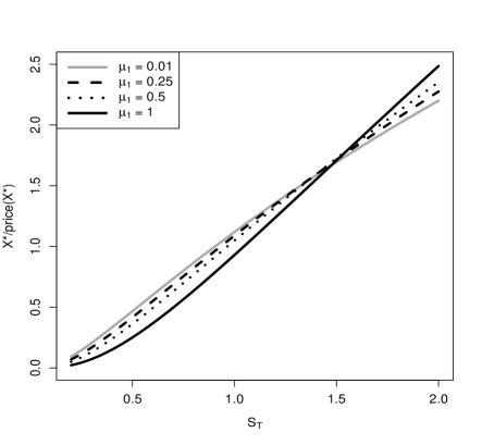
Panel A	Panel B

Figure 1: We use the parameters $S_{0}=1$, $r=0$, $T=1$ and $s=0.9$. The reference distribution function is the exponential distribution function $F_{0}(x)=1-e^{-x}$. Panel A: Price of the cost-efficient payoff $X^{\ast}$ depending on the value of the ambiguity parameter $\mu_{1}$. Panel B: Cost-efficient payoff per unit of investment for various values of $\mu_{1}$.

3.1.2 Drift and volatility uncertainty: $\mathbb{F}_{SSD}-$robust cost-efficient payoff

The real-world distribution function of $S_{T}$ is assumed to be log-normal with parameters $\log(S_{0})+(\mu-\frac{{\sigma}^{2}}{2})T$ and $\sigma^{2}T$, but now the agent faces uncertainty about the precise level of the parameters $\mu$ and $\sigma$. In particular, the agent only expects the true parameters to lie within the cube

$$\mathcal{D}^{\mu_{1},\mu_{2},\sigma_{1},s}=\left\{(\mu,\sigma)\subset\mathbb{R}^{2}\,:\,\mu_{1}\leqslant\mu\leqslant\mu_{2},\,\sigma_{1}\leqslant\sigma\leqslant s\right\}$$

for $r<\mu_{1}<\mu_{2}$ and $0<\sigma_{1}\leqslant s$, and thus she considers $\mathcal{P}=\left(\mathbb{P}^{\mu,\sigma}\right)_{(\mu,\sigma)\in\mathcal{D}^{\mu_{1},\mu_{2},\sigma_{1},s}}$ as the set of all plausible probability measures on $(\Omega,\mathcal{F})$. Under $\mathbb{P}^{\mu,\sigma}$, $S_{T}$ is log-normal with density $f^{\mu,\sigma}$, defined in Equation (3.1). In this regard, note that while $r<\mu_{1}$ is a natural assumption, there is some empirical evidence for the hypothesis that $\sigma\leqslant s$; see Table 1 in Christensen and Prabhala (1998) and Table 1 in Christensen and Hansen (2002).

Remark 3.10.

In contrast to the dynamic Black-Scholes model, in which the stock price $S_{T}$ is also log-normally distributed, we work in a static market setting. In a dynamic Black-Scholes framework where continuous trading is allowed at zero transaction cost, the absence of arbitrage opportunities implies that the volatility of the stock does not change when moving from the real-world measure to the risk-neutral measure, i.e., there does not exist uncertainty about the volatility in a dynamic Black-Scholes model. Here, however, we do not assume dynamic trading. Hence, even when call option prices reflect a risk neutral distribution function for $S_{T}$ that is log-normally distributed, the agent may have a view on the real-world distribution that is different from a log-normal and, in particular, may be unsure about the exact values for drift and volatility.

In the next proposition, we assume that

$$\frac{\mu_{1}-r}{s^{2}}\in(0,1].$$ (3.3)

For example, $s\in[0.2,\infty)$ and $(\mu_{1}-r)\in(0,0.04]$ or $s\in[0.35,\infty)$ and $(\mu_{1}-r)\in(0,0.1]$ imply Equation (3.3), that is: there are economically reasonable environments such that Equation (3.3) holds.

Proposition 3.11 ($\mathbb{F}_{SSD}-$robust cost-efficient payoff).

If $\frac{\mu_{1}-r}{s^{2}}\in(0,1]$, then it holds that $F_{S_{T}}^{\mathbb{P}^{\mu_{1},s}}\preceq_{\mathbb{F}_{SSD}}F_{S_{T}}^{\mathbb{P}^{\mu,\sigma}}$, $(\mu,\sigma)\in\mathcal{D}^{\mu_{1},\mu_{2},\sigma_{1},s}$ and conditions C3 and C4 are satisfied for the set $\mathbb{F}_{SSD}$. The least favorable measure is $\mathbb{P}^{\ast}=\mathbb{P}^{\mu_{1},s}$ with corresponding likelihood ratio $\ell^{\ast}=\ell^{\mathbb{P}^{\mu_{1},s}}$. The $\mathbb{F}_{SSD}-$robust cost-efficient payoff for the distribution function $F_{0}$ satisfying condition C1 such that $F_{0}^{-1}\circ F_{\ell^{\ast}}^{\mathbb{P}^{\ast}}$ is concave is then given by

$$X^{\ast}:=F_{0}^{-1}\left(F_{S_{T}}^{\mathbb{P}^{\mu_{1},s}}(S_{T})\right).$$ (3.4)

Proof.

For a log-normal distribution function $F$ with parameters $M$ and $V$, it holds that

$$\int_{0}^{q}F^{-1}(p)dp=\frac{e^{M+\frac{V}{2}}}{q}\ \Phi\left(\Phi^{-1}(q)-\sqrt{V}\right),\quad q\in(0,1),$$

where $\Phi$ denotes the distribution function of a standard normal random variable. It follows that

$$\int_{0}^{q}\left[F_{S_{T}}^{\mathbb{P}^{\mu_{1},s}}\right]^{-1}(p)dp =\frac{e^{\mu_{1}T}}{q}\ \Phi\left(\Phi^{-1}(q)-s\sqrt{T}\right)$$

$$\leqslant\frac{e^{\mu T}}{q}\ \Phi\left(\Phi^{-1}(q)-\sigma\sqrt{T}\right),\,\,\,q\in(0,1),\,\,\,\mu_{1}\leqslant\mu,\,\,\,\sigma\leqslant s.$$

Hence, $F_{S_{T}}^{\mathbb{P}^{\mu_{1},s}}\preceq_{\mathbb{F}_{SSD}}F_{S_{T}}^{\mathbb{P}^{\mu,\sigma}}$, $(\mu,\sigma)\in\mathcal{D}^{\mu_{1},\mu_{2},\sigma_{1},s}$. As in Section 3.1.1, let

$$\ell^{\mathbb{P}^{\mu_{1},s}}=\frac{f^{\mu_{1},s}(S_{T})}{f^{r,s}(S_{T})}=h^{\mu_{1},s}(S_{T}).$$

Hence, the likelihood ratio $\ell^{\mathbb{P}^{\mu_{1},s}}$ is strictly increasing and concave in $S_{T}$ if (3.3) is satisfied. By Proposition 2.8, conditions C3 and C4 are satisfied for the set $\mathbb{F}_{SSD}$ with least favorable measure $\mathbb{P}^{\ast}=\mathbb{P}^{\mu_{1},s}$ with likelihood ratio $\ell^{\ast}=\ell^{\mathbb{P}^{\mu_{1},s}}.$ As in Section 3.1.1, some simple calculations and Theorem 3.1 show that the robust cost-efficient payoff for the distribution function $F_{0}$ is given by (3.4). ∎

We provide an example for $F_{0}$ that make it possible to apply Proposition  3.11 to determine ${\mathbb{F}_{SSD}}-$robust cost-efficient payoffs. In this regard, observe that $F_{\ell^{\ast}}^{\mathbb{P}^{\ast}}$ in Proposition 3.11 is the log-normal distribution with parameters $\frac{1}{2}\theta^{2}$ and $\theta$ for $\theta:=\sqrt{T}\frac{\mu_{1}-r}{s}>0$.

Example 3.12.

If $F_{0}$ is the log-normal distribution with parameters $M\in\mathbb{R}$ and $V>0$, then $F_{0}^{-1}\circ F_{\ell^{\ast}}^{\mathbb{P}^{\ast}}$ in Proposition 3.11 is concave if $V\leqslant\theta$ because

$$F_{0}^{-1}\circ F_{\ell^{\ast}}^{\mathbb{P}^{\ast}}(x)=x^{\frac{V}{\theta}}\exp(-\frac{1}{2}\theta V+M),\quad x>0.$$

3.2 Robust cost-efficient payoffs in general markets using Esscher transform

Inspired by Corcuera et al. (2009), let $S_{0}>0$ and $s>0$ and $Z$ be a payoff with mean zero and variance one. Under $\mathbb{Q}$, assume that $Z$ has density $f_{Z}^{\mathbb{Q}}(x)>0$, $x\in\mathbb{R}$ and model the future stock price at date $T$ by

$$S_{T}=S_{0}e^{(r+\omega)T+s\sqrt{T}Z},$$

where $\omega\in\mathbb{R}$ is a mean correcting term, i.e., $\omega$ is chosen such that

$$e^{-rT}E_{\mathbb{Q}}\left[S_{T}\right]=S_{0}.$$

The density of $X=\log(S_{T})$ under $\mathbb{Q}$ is

$$f_{X}^{\mathbb{Q}}(x)=\frac{1}{s\sqrt{T}}f_{Z}^{\mathbb{Q}}\left(\frac{x-\log(S_{T})-(r+\omega)T}{s\sqrt{T}}\right),\quad x>0.$$

The corresponding density of $S_{T}$ under $\mathbb{Q}$ is denoted by $f_{S_{T}}^{\mathbb{Q}}$, and it holds that

$$f_{S_{T}}^{\mathbb{Q}}(x)=f_{X}^{\mathbb{Q}}(\log(x))\frac{1}{x},\quad x>0.$$

Let $h^{\ast}>0$ and $\mathcal{H}\subset[h^{\ast},\infty)$ be a set containing $h^{\ast}$ such that $E_{\mathbb{Q}}\left[(S_{T})^{h}\right]$ exists for all $h\in\text{$\mathcal{H}$}$. Define a family of probability measures $\mathcal{P}=\left(\mathbb{P}^{h}\right)_{h\in\mathcal{H}}$ as follows: $\mathbb{P}^{h}$ is a measure such that $X$ has density $f_{X}^{\mathbb{P}^{h}}$ under $\mathbb{P}^{h}$, where $f_{X}^{\mathbb{P}^{h}}$ is obtained from $f_{X}^{\mathbb{Q}}$ by applying the Esscher transform. The use of the Esscher transform can be supported by a utility maximizing argument; see Gerber and Shiu (1996). In particular, we define $\mathbb{P}^{h}$ such that

$$f_{X}^{\mathbb{P}^{h}}(x)=\frac{e^{hx}f_{X}^{\mathbb{Q}}(x)}{\int_{\mathbb{R}}e^{hy}f_{X}^{\mathbb{Q}}(y)dy}=\frac{e^{hx}f_{X}^{\mathbb{Q}}(x)}{E_{\mathbb{Q}}\left[S_{T}^{h}\right]},\quad x>0.$$

It follows that

$$f_{S_{T}}^{\mathbb{P}^{h}}(x)=\frac{x^{h}}{x}\frac{f_{X}^{\mathbb{Q}}(\log(x))}{E_{\mathbb{Q}}\left[S_{T}^{h}\right]},\quad x>0.$$

The density $f_{S_{T}}^{\mathbb{P}^{h^{\ast}}}$ crosses $f_{S_{T}}^{\mathbb{P}^{h}}$ only once from above for $h^{\ast}<h$; hence, by Denuit et al. (2005, Property 3.3.32), it follows that

$$F_{S_{T}}^{\mathbb{P}^{h^{\ast}}}\preceq_{\mathbb{F}_{FSD}}F_{S_{T}}^{\mathbb{P}^{h}}\Rightarrow F_{S_{T}}^{\mathbb{P}^{h^{\ast}}}\preceq_{\mathbb{F}_{SSD}}F_{S_{T}}^{\mathbb{P}^{h}},\quad h\in\mathcal{H}.$$

For the likelihood ratio it, holds that

$$\ell^{\mathbb{P}^{h^{\ast}}}=\frac{f_{S_{T}}^{\mathbb{P}^{h^{\ast}}}(S_{T})}{f_{S_{T}}^{\mathbb{Q}}(S_{T})}=\frac{(S_{T})^{h^{\ast}}}{E_{\mathbb{Q}}\left[(S_{T})^{h^{\ast}}\right]},$$

which is strictly increasing in $S_{T}$ as $h^{\ast}>0$ and concave if $h^{\ast}\in(0,1]$. We can apply Proposition 2.8 to show that conditions C3 and C4 are satisfied for the sets $\mathbb{F}_{FSD}$ and $\mathbb{F}_{SSD}$ with least favorable measure $\mathbb{P}^{\ast}=\mathbb{P}^{h^{*}}$ and corresponding likelihood ratio $\ell^{\ast}=\ell^{\mathbb{P}^{h^{*}}}.$ We can use Theorem  3.1 to compute the cost-efficient payoff of a distribution function $F_{0}$.

4 Robust portfolio selection

Gilboa and Schmeidler (1989) provide axioms that justify a maxmin expected utility framework to make robust decisions when there is ambiguity on the probability measure $\mathbb{P}$, i.e., when $\#{\mathcal{P}}>1.$ In this framework, Schied (2005) shows that when a least favorable measure $\mathbb{P}^{\ast}\in\mathcal{P}$ with respect to FSD ordering (e.g., the stochastic integral ordering induced by the set $\mathbb{F}_{FSD}$ as defined in Section 3) exists, an optimal portfolio can be derived. In this section, we extend the work of Schied (2005) in two different ways. First, we account for preferences beyond expected utility. Specifically, we derive optimal portfolios for robust preferences that are in accord with expected utility theory, rank dependent utility theory and Yaari’s dual theory. Second, assuming the existence of a least favorable measure $\mathbb{P}^{\ast}$ with respect to a general stochastic integral ordering induced by some set $\mathbb{F}$, not necessarily identical to $\mathbb{F}_{FSD}$, we derive the optimal portfolio. Specifically, we derive optimal portfolios when a least favorable measure $\mathbb{P}^{\ast}\in\mathcal{P}$ with respect to SSD ordering exists (see Proposition 2.8 for a sufficient condition) and the target distribution $F_{0}$ is sufficiently light tailed (see Remark 3.4).

4.1 Family consistent preferences

A preference $W$ is defined as a functional from the set of payoffs $\mathcal{X}$ to the real line (He et al. (2017), Assa and Zimper (2018)). Under preference $W$, the payoff $Y$ is preferred to $X$ if $W(X)\leqslant W(Y)$. In general, $W$ may depend on the different measures $\mathbb{P}\in\mathcal{P}$ in a complicated way. In what follows, we denote a preference that depends solely on some $\mathbb{P}\in\mathcal{P}$ by $W_{\mathbb{P}}$.

Definition 4.1.

Let $\left(W_{\mathbb{P}}\right)_{\mathbb{P}\in\mathcal{P}}$ be a family of preferences. The preference $W_{\mathbb{P}}$, $\mathbb{P}\in\mathcal{P}$ is called $\mathbb{P}-$law invariant if $F_{X}^{\mathbb{P}}=F_{Y}^{\mathbb{P}}$ implies that $W_{\mathbb{P}}(X)=W_{\mathbb{P}}(Y)$. The family $\left(W_{\mathbb{P}}\right)_{\mathbb{P}\in\mathcal{P}}$ is called law invariant if each individual preference $W_{\mathbb{P}}$ is $\mathbb{P}-$law invariant.

Example 4.2.

A standard example of a $\mathbb{P}-$law invariant preference is $W_{\mathbb{P}}(X)=E_{\mathbb{P}}[u(X)]$ for some increasing utility function $u$. In this case, $W(X)=\underset{\mathbb{P}\in\mathcal{P}}{\inf}\,W_{\mathbb{P}}(X)$ amounts to the worst-case expected utility, commonly called robust expected utility, which was introduced in Gilboa and Schmeidler (1989). It is also referred to a robust utility functional in Schied et al. (2009).

To the best of our knowledge, the next definition is new to the literature. It will be helpful in solving robust portfolio choice problems.

Definition 4.3.

Let $(W_{\mathbb{P}})_{\mathbb{P}\in\mathcal{P}}$ be a family of preferences. Let $\mathcal{Y}\subset\mathcal{X}$. The family of preferences $(W_{\mathbb{P}})_{\mathbb{P}\in\mathcal{P}}$ is called $\mathbb{F}-$family consistent on $\mathcal{Y}$ with respect to $\mathbb{P}^{\ast}\in\mathcal{P}$ if for all $Y\in\mathcal{Y}$ the inequality

$$F_{Y}^{\mathbb{P}^{\ast}}\preceq_{\mathbb{F}}F_{Y}^{\mathbb{P}},\quad\mathbb{P}\in\mathcal{P}$$

implies that

$$W_{\mathbb{P}^{\ast}}(Y)\leqslant W_{\mathbb{P}}(Y),\quad\mathbb{P}\in\mathcal{P}.$$

$\mathbb{F}-$family consistency of $(W_{\mathbb{P}})_{\mathbb{P}\in\mathcal{P}}$ with respect to some $\mathbb{P}^{\ast}\in\mathcal{P}$ has the following interpretation: if a measure $\mathbb{P}^{\ast}$ yields the most pessimistic view of any payoff $Y$ w.r.t. the stochastic ordering induced by some set $\mathbb{F}$, then the preference under that measure is the lowest as well.

Next, we discuss some examples. Let $\mathcal{Y}\subset\mathcal{X}$ be a set of payoffs and let $\mathcal{D}$ be the set of cumulative distribution functions induced by $\mathcal{Y}$, i.e.,

$$\mathcal{D}=\{F_{Y}^{\mathbb{P}}:\,Y\in\mathcal{Y},\,\mathbb{P}\in\mathcal{P}\}.$$

Let us consider an agent taking into account a family of law invariant preferences $(W_{\mathbb{P}})_{\mathbb{P}\in\mathcal{P}},$ i.e.,

$$W_{\mathbb{P}}(Y)=w(F_{Y}^{\mathbb{P}})$$ (4.1)

for some well defined $w:\mathcal{D}\rightarrow\mathbb{R}$. If $w$ respects integral stochastic ordering, i.e.,

$$F\preceq_{\mathbb{F}}G\Rightarrow w(F)\leqslant w(G),\quad F,G\in\mathcal{D},$$ (4.2)

then $(W_{\mathbb{P}})_{\mathbb{P}\in\mathcal{P}}$ is $\mathbb{F}-$family consistent on $\mathcal{Y}$ with respect to $\mathbb{P}^{\ast}\in\mathcal{P}$. We provide some specific examples in the contexts of expected utility theory, Yaari’s dual theory of choice and rank-dependent expected utility theory:

Example 4.4.

Let $u:\mathbb{R}_{+}\to\mathbb{R}$. Let $\phi:[0,1]\rightarrow[0,1]$ with $\phi(0)=0$ and $\phi(1)=1$. For a given distribution function $F$, define

$$w^{\text{EUT}}(F) =\int_{\mathbb{R_{+}}}u(x)dF$$

$$w^{\text{Yaari}}(F) =\int_{\mathbb{R_{+}}}\phi(1-F(x))dx$$

$$w^{\text{RDEU}}(F) =\int_{\mathbb{R_{+}}}u(x)d(1-\phi(1-F(x)),$$

where we tacitly assume that all integrals exist. It is straightforward to show that when $u$ and $\phi$ are non-decreasing, it holds that the family of preferences induced by $w^{\text{EUT}}$, $w^{\text{Yaari}}$ or $w^{\text{RDEU}}$ as in (4.1) is $\mathbb{F}_{FSD}-$family consistent on $\mathcal{Y}$ where $\mathcal{Y}$ is restricted to contain random variables such that all relevant integrals exist. Furthermore, if $u$ is strictly increasing and concave and $\phi$ is strictly increasing, continuously differentiable and convex, we obtain that such a family is a $\mathbb{F}_{SSD}-$family consistent on $\mathcal{Y}$; see Yaari (1987), Wang and Young (1998), He et al. (2017) and Ryan (2006).

Remark 4.5.

One could allow the function $w$ in (4.1) to depend on $\mathbb{P}$, i.e., define $W_{\mathbb{P}}(Y)=w_{\mathbb{P}}(F_{Y}^{\mathbb{P}})$ for some $w_{\mathbb{P}}:\mathcal{D}\rightarrow\mathbb{R}$, $\mathbb{P}\in\mathcal{P}$. The family of preferences is then $\mathbb{F}-$family consistent on $\mathcal{Y}$ with respect to $\mathbb{P}^{\ast}\in\mathcal{P}$ if both

$$w_{\mathbb{P}^{\ast}}(F)\leqslant w_{\mathbb{P}}(F),\quad F\in\mathcal{D},\quad\mathbb{P}\in\mathcal{P}$$

and (4.2) holds. To see this, let $Y\in\mathcal{Y}$ with $F_{Y}^{\mathbb{P}^{\ast}}\leqslant F_{Y}^{\mathbb{P}}$ for all $\mathbb{P}\in\mathcal{P}$. It follows that

$$W_{\mathbb{P}^{\ast}}(Y)=w_{\mathbb{P}^{\ast}}\left(F_{Y}^{\mathbb{P}^{\ast}}\right)\leqslant w_{\mathbb{P}}\left(F_{Y}^{\mathbb{P}^{\ast}}\right)\leqslant w_{\mathbb{P}}\left(F_{Y}^{\mathbb{P}}\right)=W_{\mathbb{P}}(Y).$$

4.2 Optimal portfolio for robust preferences

Inspired by Gilboa and Schmeidler (1989) and Schied (2005), we consider the following problem:

Problem 2.

Let $x_{0}>0$ be the initial wealth. Let $\left(W_{\mathbb{P}}\right)_{\mathbb{P}\in\mathcal{P}}$ be a family of preferences. We consider the robust maximization problem

$$\max_{X\in\mathcal{Y}_{(W_{\mathbb{P}})_{\mathbb{P}\in\mathcal{P}}}^{x_{0}}}\inf_{\mathbb{P}\in\mathcal{P}}W_{\mathbb{P}}(X),$$ (4.3)

where $\mathcal{Y}_{(W_{\mathbb{P}})_{\mathbb{P}\in\mathcal{P}}}^{x_{0}}=\bigcap_{\mathbb{P}\in\mathcal{P}}\mathcal{Y}_{W_{\mathbb{P}}}^{x_{0}}$ and

$$\mathcal{Y}_{W_{\mathbb{P}}}^{x_{0}}:=\left\{X\in\mathcal{X}\,:W_{\mathbb{P}}[X]\in\mathbb{R},\,e^{-rT}E_{\mathbb{Q}}\left[X\right]\leqslant x_{0}\right\},\quad\mathbb{P}\in\mathcal{P}.$$ (4.4)

It turns out that under certain conditions a solution to the robust optimization problem (4.3) can be found as a solution to a maximization problem under a single measure $\mathbb{P}\in\mathcal{P}$.

Problem 3.

Let $x_{0}>0$ be the initial wealth. Let $W_{\mathbb{P}}$, ${\mathbb{P}\in\mathcal{P}}$ be a preference. We consider the maximization problem

$$\max_{X\in\mathcal{Y}_{W_{\mathbb{P}}}^{x_{0}}}W_{\mathbb{P}}(X).$$ (4.5)

Under the assumption of the existence of a least favorable measure with respect to FSD ordering, Schied (2005) showed that in order to solve the robust maximization problem (4.3) for preferences $\left(W_{\mathbb{P}}\right)_{\mathbb{P}\in\mathcal{P}}$, ${W}_{\mathbb{P}}(x)=E_{\mathbb{P}}[u(X)]$, it actually suffices to solve the single measure maximization problem (4.5). The following theorem generalizes this result beyond the expected utility setting to a general law invariant family of preferences $\left(W_{\mathbb{P}}\right)_{\mathbb{P}\in\mathcal{P}}$. The theorem is illustrated in Section 4.3, where we consider a robust rank-dependent expected utility maximization problem for an investor with ambiguity on the trend and/or volatility of the risky asset.

Theorem 4.6.

Let $\mathbb{F}=\mathbb{F}_{FSD}$. Given conditions C3 and C4, assume that $\left(W_{\mathbb{P}}\right)_{\mathbb{P}\in\mathcal{P}}$ is a law invariant and $\mathbb{F}_{FSD}-$consistent family of preferences on $\mathcal{Y}_{(W_{\mathbb{P}})_{\mathbb{P}\in\mathcal{P}}}^{x_{0}}$ with respect to $\mathbb{P}^{\ast}\in\mathcal{P}$. Assume that the maximization problem (4.5) under $\mathbb{P}^{\ast}$ has a solution $\tilde{X}\in\mathcal{Y}_{(W_{\mathbb{P}})_{\mathbb{P}\in\mathcal{P}}}^{x_{0}}.$ Then it holds that

$$\underset{X\in\mathcal{Y}_{(W_{\mathbb{P}})_{\mathbb{P}\in\mathcal{P}}}^{x_{0}}}{\max}\,\underset{\mathbb{P}\in\mathcal{P}}{\inf}\,W_{\mathbb{P}}(X)=\underset{X\in\mathcal{Y}_{W_{\mathbb{P^{\ast}}}}^{x_{0}}}{\max}\,W_{\mathbb{P}^{\ast}}(X).$$

Proof.

Let $h\in\mathbb{F}_{FSD}$ such that $h(\ell^{\ast})\in\mathcal{Y}_{(W_{\mathbb{P}})_{\mathbb{P}\in\mathcal{P}}}^{x_{0}}$. Then, it holds by the $\mathbb{F}_{FSD}-$family consistency, condition C3 and (2.4) that

$$W_{\mathbb{P}^{\ast}}(h(\ell^{\ast}))\leqslant\underset{\mathbb{P}\in\mathcal{P}}{\inf}\,W_{\mathbb{P}}(h(\ell^{\ast})).$$ (4.6)

Let

$$X^{\ast}=\left[F_{\tilde{X}}^{\mathbb{P}^{\ast}}\right]^{-1}\left(F_{\ell^{\ast}}^{\mathbb{P}^{\ast}}(\ell^{\ast})\right).$$

Then $X^{\ast}$ solves the standard cost-efficiency problem for $F_{\tilde{X}}^{\mathbb{P}^{\ast}}$ and thus $E_{\mathbb{Q}}[X^{\ast}]\leqslant E_{\mathbb{Q}}[\tilde{X}]$ and $F_{\tilde{X}}^{\mathbb{P}^{\ast}}=F_{X^{\ast}}^{\mathbb{P}^{\ast}}$; hence, by the law invariance of $\left(W_{\mathbb{P}}\right)_{\mathbb{P}\in\mathcal{P}}$, it holds that $X^{\ast}\in\mathcal{Y}_{(W_{\mathbb{P}})_{\mathbb{P}\in\mathcal{P}}}^{x_{0}}$. It further holds that $X^{\ast}$ is a non-decreasing function of $\ell^{\ast}$. It follows by (4.6) that

$$\underset{X\in\mathcal{Y}_{W_{\mathbb{P^{\ast}}}}^{x_{0}}}{\max}\,W_{\mathbb{P}^{\ast}}(X) =W_{\mathbb{P}^{\ast}}(\tilde{X})=W_{\mathbb{P}^{\ast}}(X^{\ast})$$

$$\leqslant\underset{\mathbb{P}\in\mathcal{P}}{\inf}\,W_{\mathbb{P}}(X^{\ast})$$

$$\leqslant\underset{X\in\mathcal{Y}_{(W_{\mathbb{P}})_{\mathbb{P}\in\mathcal{P}}}^{x_{0}}}{\max}\,\underset{\mathbb{P}\in\mathcal{P}}{\inf}\,W_{\mathbb{P}}(X)$$

$$\leqslant\underset{X\in\mathcal{Y}_{(W_{\mathbb{P}})_{\mathbb{P}\in\mathcal{P}}}^{x_{0}}}{\max}\,W_{\mathbb{P}^{\ast}}(X)$$

$$\leqslant\underset{X\in\mathcal{Y}_{W_{\mathbb{P^{\ast}}}}^{x_{0}}}{\max}\,W_{\mathbb{P}^{\ast}}(X),$$

where the last inequality follows by $\mathcal{Y}_{(W_{\mathbb{P}})_{\mathbb{P}\in\mathcal{P}}}^{x_{0}}\subset\mathcal{Y}_{W_{\mathbb{P^{\ast}}}}^{x_{0}}$. ∎

From Theorem 4.6, it follows immediately that solving robust preference maximization problems may reduce to solving an optimization problem under a single probability measure. The following example illustrates this consequence.

Example 4.7.

Assume $\mathbb{F}=\mathbb{F}_{FSD}$ and that conditions C3 and C4 are satisfied. Let $W_{\mathbb{P}}(F)=w(F_{Y}^{\mathbb{P}})$ as in (4.1), where $w\in\{w^{\text{EUT}},w^{\text{Yaari}},w^{\text{RDEU}}\}$ as in Example 4.4. Assuming a solution to (4.5) under $\mathbb{P}^{\ast}\in\mathcal{P}$ exists, then it follows that

$$\underset{X\in\mathcal{Y}_{(W_{\mathbb{P}})_{\mathbb{P}\in\mathcal{P}}}^{x_{0}}}{\max}\,\underset{\mathbb{P}\in\mathcal{P}}{\inf}\,W_{\mathbb{P}}(X)=\underset{X\in\mathcal{Y}_{W_{\mathbb{P^{\ast}}}}^{x_{0}}}{\max}\,W_{\mathbb{P}^{\ast}}(X).$$

The main assumption in Theorem 4.6 that is needed to solve the robust maximization problem (4.3) in the case of a family of law invariant preferences $\left(W_{\mathbb{P}}\right)_{\mathbb{P}\in\mathcal{P}}$ is the existence of a least favorable measure $\mathbb{P}^{\ast}$ with respect to $\mathbb{F}_{FSD}$. In the following theorem we show that it is possible to weaken this assumption in that we only require existence of a least favorable measure $\mathbb{P}^{\ast}$ with respect to some $\mathbb{F}\subset\mathbb{F}_{FSD}$, e.g., $\mathbb{F}=\mathbb{F}_{SSD}$. The theorem is illustrated in Section 4.3, where we consider a robust rank-dependent expected utility maximization problem for an investor who faces ambiguity on expected return and volatility of the risky asset.

Theorem 4.8.

Consider a given set $\mathbb{F}.$ Given conditions C3 and C4, assume that the maximization problem (4.5) under $\mathbb{P}^{\ast}$ has a solution $\tilde{X}\in\mathcal{Y}_{(W_{\mathbb{P}})_{\mathbb{P}\in\mathcal{P}}}^{x_{0}}$, which can $\mathbb{P}^{\ast}-$a.s. be expressed as $f(\ell^{\ast})$ for some $f\in\mathbb{F}$. Further, assume that $\left(W_{\mathbb{P}}\right)_{\mathbb{P}\in\mathcal{P}}$ is $\mathbb{F}-$family consistent on $\mathcal{Y}_{(W_{\mathbb{P}})_{\mathbb{P}\in\mathcal{P}}}^{x_{0}}$ with respect to $\mathbb{P}^{\ast}$. Then it holds that

$$\underset{X\in\mathcal{Y}_{(W_{\mathbb{P}})_{\mathbb{P}\in\mathcal{P}}}^{x_{0}}}{\max}\,\underset{\mathbb{P}\in\mathcal{P}}{\inf}\,W_{\mathbb{P}}(X)=\underset{X\in\mathcal{Y}_{W_{\mathbb{P^{\ast}}}}^{x_{0}}}{\max}\,W_{\mathbb{P}^{\ast}}(X).$$

Proof.

Let $h\in\mathbb{F}$ such that $h(\ell^{\ast})\in\mathcal{Y}_{(W_{\mathbb{P}})_{\mathbb{P}\in\mathcal{P}}}^{x_{0}}$. Then, (4.6) holds true by the $\mathbb{F}-$family consistency and (2.4). By assumption, $\tilde{X}=f(\ell^{\ast})$, $\mathbb{P}^{\ast}-$a.s. for some $f\in\mathbb{F}$. Hence, it holds that

$$\underset{X\in\mathcal{Y}_{W_{\mathbb{P^{\ast}}}}^{x_{0}}}{\max}\,W_{\mathbb{P}^{\ast}}(X) =W_{\mathbb{P}^{\ast}}(\tilde{X})$$

$$\leqslant\underset{\mathbb{P}\in\mathcal{P}}{\inf}\,W_{\mathbb{P}}(\tilde{X})$$

$$\leqslant\underset{X\in\mathcal{Y}_{(W_{\mathbb{P}})_{\mathbb{P}\in\mathcal{P}}}^{x_{0}}}{\max}\,\underset{\mathbb{P}\in\mathcal{P}}{\inf}\,W_{\mathbb{P}}(X)$$

$$\leqslant\underset{X\in\mathcal{Y}_{(W_{\mathbb{P}})_{\mathbb{P}\in\mathcal{P}}}^{x_{0}}}{\max}\,W_{\mathbb{P}^{\ast}}(X)$$

$$\leqslant\underset{X\in\mathcal{Y}_{W_{\mathbb{P^{\ast}}}}^{x_{0}}}{\max}\,W_{\mathbb{P}^{\ast}}(X),$$

in which the last inequality follows by $\mathcal{Y}_{(W_{\mathbb{P}})_{\mathbb{P}\in\mathcal{P}}}^{x_{0}}\subset\mathcal{Y}_{W_{\mathbb{P^{\ast}}}}^{x_{0}}$. ∎

Note that, as compared to the statements in Theorem 4.6, in Theorem 4.8 the $W_{\mathbb{P}}$ do not need to be law-invariant. Moreover, as long as the solution can be expressed as a certain function of the likelihood ratio $\ell^{\ast}$, the preferences do not need to be increasing, i.e., $X\leqslant Y$ does not need to imply $W_{\mathbb{P}}(X)\leqslant W_{\mathbb{P}}(Y).$ As pointed out, Theorem 4.8 is applicable, in particular, for the case $\mathbb{F}=\mathbb{F}_{SSD}$. However, the requirement that $\tilde{X}\in\mathcal{Y}_{(W_{\mathbb{P}})_{\mathbb{P}\in\mathcal{P}}}^{x_{0}}$ can be $\mathbb{P}^{\ast}-$a.s. expressed as $h(\ell^{\ast})$ for some $h\in\mathbb{F}_{SSD}$ is equivalent to $h$ being increasing and concave. This property is difficult to verify ex-ante. Hereafter, we show that in the case in which $W_{\mathbb{P}}$ is an expected utility, this condition translates into an easy-to-verify condition on the utility function. We formulate the following theorem.

Theorem 4.9.

Let $\mathbb{P}\in\mathcal{P}$ with likelihood ratio $\ell^{\mathbb{P}}$. Let $u:\mathbb{R}_{+}\rightarrow\mathbb{R}$ be a differentiable, concave and strictly increasing utility function such that $u^{\prime}$ is strictly decreasing. If the maximization problem (4.5) under $\mathbb{P}$ has a solution, then the solution is a non-decreasing and concave function of $\ell^{\mathbb{P}}$ if and only if $\frac{1}{u^{\prime}}$ is convex. If $u$ is three times differentiable, $\frac{1}{u^{\prime}}$ is convex if and only if

$$a(x)\geqslant\frac{p(x)}{2},$$ (4.7)

in which $a(x):=-\frac{u^{\prime\prime}(x)}{u^{\prime}(x)}$ refers to the absolute risk aversion measure and $p(x):=-\frac{u^{\prime\prime\prime}(x)}{u^{\prime\prime}(x)}$ to the absolute prudence.

Proof.

By Lemma 2 in Bernard et al. (2015), the solution to (4.5) is unique and given by $[u^{\prime}]^{-1}\left(\frac{c_{0}}{\ell^{\mathbb{P}}}\right)$ for some $c_{0}>0$. See also Merton (1971) for a proof in a context in which Inada’s conditions are satisfied. Note that $u^{\prime}>0$ and that $\frac{1}{u^{\prime}}$ is strictly increasing. Observe that the inverse of $\frac{1}{u^{\prime}}$ is $x\mapsto[u^{\prime}]^{-1}(\frac{1}{x})$, which is hence also strictly increasing. The inverse of a convex (concave) and strictly increasing function is concave (convex). For the second assertion, observe that $u^{\prime\prime}<0$ and that a function is convex on an open interval if and only if its second derivative is non-negative. Then (4.7) follows immediately. ∎

Remark 4.10.

Maggi et al. (2006) have shown that $a(x)>p(x)$ if and only if the utility has increasing absolute risk aversion, which is somewhat unusual (it is typically assumed that agents have decreasing absolute risk aversion given that they become less risk averse as their wealth increases). Here, our condition (4.7) is not incompatible with decreasing absolute risk aversion due to the factor $\frac{1}{2}$.

Condition (4.7) has appeared several times in the literature. It has been found to play a role in the context of insurance models in Bourlès (2017), but it also appeared as a condition in the opening of a new asset market (Gollier and Kimball (1996)), when there is uncertainty on the size (Gollier et al. (2000)) or the probability of losses (Gollier (2002)) and under contingent auditing (Sinclair-Desgagné and Gabel (1997)). Further interpretation of this condition and, in particular, of the degree of concavity of the inverse of the marginal utility can be found in Bourlès (2017). This condition also appears in Varian (1985) in the context of portfolio selection under ambiguity.

Example 4.11.

As an illustration of Theorem 4.9, we provide two utility functions, which are differentiable, concave and strictly increasing functions such that one over the marginal utility is convex.

• The exponential utility for risk-averse agents: $u:\mathbb{R}_{+}\rightarrow\mathbb{R},\,x\mapsto 1-e^{-\lambda x},$ for $\lambda>0$. It holds that $\frac{1}{u^{\prime}(x)}=e^{\lambda x}$, which is strictly increasing and convex.

• CRRA utility: $u:\mathbb{R}_{+}\rightarrow\mathbb{R},\,x\mapsto\frac{x^{1-\eta}}{1-\eta},$ for $\eta>1$. It holds that $\frac{1}{u^{\prime}(x)}=x^{\eta}$, which is strictly increasing and convex.

4.3 Rank-dependent utility in log-normal markets

We now discuss some examples to illustrate Section 4.2 in a log-normal market setting with uncertainty on the drift and volatility. In particular, we explicitly solve a robust rank-dependent expected utility problem using Theorems 4.6 and 4.8. As in Section 3.1.2, we assume that the real-world distribution of $S_{T}$ is log-normal with parameters $\log(S_{0})+(\mu-\frac{\sigma^{2}}{2})T$ and $\sigma^{2}T$ and that the investor has uncertainty on the trend and potentially also the volatility. She may expect the true parameters to lie within the cube

$$\mathcal{D}^{\mu_{1},\mu_{2},\sigma_{1},s}=\left\{(\mu,\sigma)\subset\mathbb{R}^{2}\,:\,\mu_{1}\leqslant\mu\leqslant\mu_{2},\,\sigma_{1}\leqslant\sigma\leqslant s\right\}$$

for $r<\mu_{1}<\mu_{2}$ and $0<\sigma_{1}\leqslant s$. The investor thus considers $\mathcal{P}=\left(\mathbb{P}^{\mu,\sigma}\right)_{(\mu,\sigma)\in\mathcal{D}^{\mu_{1},\mu_{2},\sigma_{1},s}}$ as the set of all plausible probability measures on $(\Omega,\mathcal{F})$. Note that if $\sigma_{1}=s,$ the investor only faces drift ambiguity; otherwise, she considers ambiguity on both trend and volatility. Under $\mathbb{P}^{\mu,\sigma}$, $S_{T}$ is log-normal with density $f^{\mu,\sigma}$, defined in Equation (3.1). In the next example, $\Phi$ is the standard normal distribution function.

Example 4.12.

Let $U(x)=\frac{x^{1-\eta}}{1-\eta}$, $x\geqslant 0$ for $\eta\in(0,1)$ be the CRRA utility function. Let $\gamma\in\mathbb{R}$ and let $w(u)=\Phi(\Phi^{-1}(u)+\gamma)$, $u\in[0,1]$ denote the so-called Wang transform, which is increasing concave if $\gamma>0$ and increasing convex if $\gamma<0$. Consider the following portfolio choice problem; in which the investor maximizes her expected rank-dependent utility:

$$\max_{X\in\mathcal{Y}_{W_{\mathbb{P}^{\mu,\sigma}}}^{x_{0}}}\int_{0}^{\infty}U(x)d(1-w(1-F_{X}^{\mathbb{P}^{\mu,\sigma}}(x)))$$ (4.8)

where $x_{0}>0$ is the initial wealth and $(\mu,\sigma)\in\mathcal{D}^{\mu_{1},\mu_{2},\sigma_{1},s}$. Let $\theta:=\sqrt{T}\frac{\mu-r}{\sigma}$. The solution to (4.8) is given by

$$X_{\mu,\sigma}^{\ast}:=\begin{cases}\lambda^{-\frac{1}{\eta}}\exp\left(\frac{rT}{\eta}-\frac{1}{2}\frac{\gamma}{\eta}(\theta+\gamma)\right)\left(\ell^{\mathbb{P}}\right)^{\frac{\gamma}{\theta\eta}+\frac{1}{\eta}}&,\gamma>-\theta\\ \lambda^{-\frac{1}{\eta}}&\text{, otherwise,}\end{cases}$$ (4.9)

where $\lambda$ depends on $\eta$, $\gamma$ and $\theta$, see Equations (4.11), (4.12) and (4.13). The solution to the robust rank-dependent utility problem

$$\max_{X\in\mathcal{Y}_{(W_{\mathbb{P}})_{\mathbb{P}\in\mathcal{P}}}^{x_{0}}}\inf_{\mathbb{P}\in\mathcal{P}}\int_{0}^{\infty}U(x)d(1-w(1-F_{X}^{\mathbb{P}}(x)))dx$$ (4.10)

is given by $X_{\mu_{1},s}^{\ast}$ if there is no ambiguity on the volatility, i.e., when $\sigma_{1}=s$. If there is ambiguity on the volatility, $\gamma<0$ and $\frac{\mu_{1}-r}{s^{2}}\in(0,1]$, then $X_{\mu_{1},s}^{\ast}$ still solves (4.10).

Proof.

We first prove that $X_{\mu,\sigma}^{\ast}$ solves (4.8). Let $\mathbb{P}=\mathbb{P}^{\mu,\sigma}$. The state price $\xi^{\mathbb{P}}:=\frac{e^{-rT}}{\ell^{\mathbb{P}}}$ is log-normally distributed with parameters $-rT-\frac{1}{2}\theta^{2}$ and $\theta>0$, see Equation (3.2). Hence, as $\mu>r$, it holds that

$$F_{\xi^{\mathbb{P}}}^{\mathbb{P}}(x) =\mathbb{P}\left(\xi^{\mathbb{P}}\leqslant x\right)=\Phi\left(\frac{\log(x)+rT+\frac{1}{2}\theta^{2}}{\theta}\right),\quad x>0$$

and

$$\left[F_{\xi^{\mathbb{P}}}^{\mathbb{P}}\right]^{-1}(p)=\exp\left(\Phi^{-1}(p)\theta-rT-\frac{1}{2}\theta^{2}\right),\quad p\in(0,1).$$

Let

$$H(z)=-\int_{0}^{w^{-1}(1-z)}\left[F_{\xi^{\mathbb{P}}}^{\mathbb{P}}\right]^{-1}(t)dt,\quad z\in[0,1].$$

The solution to the classical rank-utility problem (4.8) is well-known (see for instance Theorem 4.1 in Xu (2016) or Section 3.2 in Rüschendorf and Vanduffel (2020)), and is given by

$$X_{\mu,\sigma}^{\ast}=[U^{\prime}]^{-1}\left(\lambda\hat{H}^{\prime}\left(1-w\left(F_{\xi^{\mathbb{P}}}^{\mathbb{P}}\left(\xi^{\mathbb{P}}\right)\right)\right)\right),$$

where $\lambda$ is determined by $E_{\mathbb{P}}\left[\xi^{\mathbb{P}}X_{\mu,\sigma}^{\ast}\right]=x_{0}$ and $\hat{H}$ is the concave envelope of $H$. Using $w^{\prime}(u)=\frac{\Phi^{\prime}(\Phi^{-1}(u)+\gamma)}{\Phi^{\prime}(\Phi^{-1}(u))}$ , after some calculations, we obtain that

$$H^{\prime}(z) =\frac{\left[F_{\xi^{\mathbb{P}}}^{\mathbb{P}}\right]^{-1}(w^{-1}(1-z))}{w^{\prime}(w^{-1}(1-z))}=\exp\left(\Phi^{-1}(1-z)(\gamma+\theta)-rT-\frac{1}{2}(\gamma+\theta)^{2}\right).$$

We distinguish two cases to find a more explicit expression for $X_{\mu,\sigma}^{\ast}$. Case 1: $\gamma+\theta>0$. Then, $H^{\prime}$ is non-increasing and hence $H$ is concave and equal to $\hat{H}$. As $[U^{\prime}]^{-1}(y)=y^{-\frac{1}{\eta}}$, it is easy to see that

$$X_{\mu,\sigma}^{\ast} =\lambda^{-\frac{1}{\eta}}\exp\left(-\frac{rT\gamma}{\theta\eta}-\frac{1}{2}\frac{\gamma}{\eta}(\theta+\gamma)\right)\left(\xi^{\mathbb{P}}\right)^{-\frac{\gamma}{\theta\eta}-\frac{1}{\eta}}$$

$$=\lambda^{-\frac{1}{\eta}}\exp\left(\frac{rT}{\eta}-\frac{1}{2}\frac{\gamma}{\eta}(\theta+\gamma)\right)\left(\ell^{\mathbb{P}}\right)^{\frac{\gamma}{\theta\eta}+\frac{1}{\eta}}.$$

If $1-\frac{\gamma}{\theta\eta}-\frac{1}{\eta}=0$, then $\xi^{\mathbb{P}}X_{\mu,\sigma}^{\ast}$ is constant and it holds that

$$\lambda=x_{0}^{-\eta}\exp\left(-\frac{rT\gamma}{\theta}-\frac{1}{2}\gamma(\theta+\gamma)\right).$$ (4.11)

Otherwise, $\xi^{\mathbb{P}}X_{\mu,\sigma}^{\ast}$ is log-normally distributed and it follows that

$$\lambda=x_{0}^{-\eta}\exp\left(rT(1-\eta)+\frac{1}{2}\left(\theta^{2}(1-\eta)+\gamma^{2}+(\theta\eta-(\gamma+\theta))^{2}\right)\right).$$ (4.12)

Case 2: Assume $\gamma+\theta\leqslant 0$. Then, $H$ is convex. Note that $H(0)=-1$ and $H(1)=0$. As $H$ is convex, the concave envelope $\hat{H}$ of $H$ is given by $\hat{H}(x)=x-1$. Then $\hat{H}^{\prime}\equiv 1$ and

$$X_{\mu,\sigma}^{\ast}=[U^{\prime}]^{-1}\left(\lambda\right)=\lambda^{-\frac{1}{\eta}}.$$

Therefore, $\xi^{\mathbb{P}}X_{\mu,\sigma}^{\ast}=\lambda^{-\frac{1}{\eta}}\xi^{\mathbb{P}}$, and hence

$$\lambda=x_{0}^{-\eta}e^{-rT\eta}.$$ (4.13)

Assume that there is no ambiguity on the volatility, i.e., $\sigma_{1}=s$. Section 3.1.1 shows that the least favorable measure with respect to $\mathbb{F}_{FSD}$ is given by $\mathbb{P}^{\ast}=\mathbb{P}^{\mu_{1},s}$ with corresponding likelihood ratio $\ell^{\ast}=\ell^{\mathbb{P}^{\mu_{1},s}}$. By Example 4.4, the preference in (4.10) is $\mathbb{F}_{FSD}-$family consistent and Theorem 4.6 shows that $X_{\mu,\sigma}^{\ast}$ solves the robust rank-dependent utility problem (4.10). Lastly, assume that there is ambiguity on the volatility. If $\frac{\mu_{1}-r}{s^{2}}\in(0,1]$, Proposition 3.11 shows that the least favorable measure with respect to $\mathbb{F}_{SSD}$ is also $\mathbb{P}^{\ast}$. If $\gamma<0$, $X_{\mu,\sigma}^{\ast}$ is a concave and non-decreasing function of $\ell^{\ast}$. By Example 4.4, the preference in (4.10) is $\mathbb{F}_{SSD}-$family consistent. Apply Theorem 4.8 to show that also in this case, $X_{\mu,\sigma}^{\ast}$ solves the robust rank-dependent utility problem (4.10). ∎

To better understand the solution in Example 4.12, we “rationalize” the solution as in Bernard et al. (2015), i.e., we show that the optimal investment strategy in the robust rank-dependent setting also solves an expected utility maximization problem. Example 4.13 shows that the solution to the expected rank-dependent utility problems (4.8) and (4.10) involving a Wang transform with parameter $\gamma$ and a CRRA utility function with parameter $\eta$ can be rationalized by a CRRA utility with parameter $\frac{\eta\theta}{\gamma+\theta}$.

Example 4.13.

Let $(\mu,\sigma)\in\mathcal{D}^{\mu_{1},\mu_{2},\sigma_{1},s}$, $X_{\mu,\sigma}^{\ast}$, $\theta$, $x_{0}$ and $\mathcal{Y}_{W_{\mathbb{P}^{\mu,\sigma}}}^{x_{0}}$ as in Example 4.12, such that $\gamma>-\theta$ and $\eta\theta\neq\gamma+\theta$. $X_{\mu,\sigma}^{\ast}$ solves the following expected utility maximization problem:

$$\max_{X\in\mathcal{Y}_{W_{\mathbb{P}^{\mu,\sigma}}}^{x_{0}}}\int_{0}^{\infty}u(x)dF_{X}^{\mathbb{P}^{\mu,\sigma}}(x)$$

for the utility function

$$u(x)=\frac{1}{1-\frac{\eta\theta}{\gamma+\theta}}x^{1-\frac{\eta\theta}{\gamma+\theta}}.$$ (4.14)

The function $u:\mathbb{R}_{+}\to\mathbb{R}$ is non-decreasing and concave.

Proof.

Note that $\gamma>-\theta$ implies $\frac{\gamma}{\theta\eta}+\frac{1}{\eta}\neq 0$. Let $\mathbb{P}=\mathbb{P}^{\mu,\sigma}$. Let $\xi^{\mathbb{P}}:=\frac{e^{-rT}}{\ell^{\mathbb{P}}}$. As in Bernard et al. (2015), let $c>0$ and define

$$\tilde{u}(x)=\int_{c}^{x}\left[F_{\xi^{\mathbb{P}}}^{\mathbb{P}}\right]^{-1}\left(1-F_{X_{\mu,\sigma}^{\ast}}^{\mathbb{P}}(y)\right)dy,\quad x\in\mathbb{R}_{+}.$$

$X_{\mu,\sigma}^{\ast}$ is log-normally distributed. It follows that

$$\left[F_{\xi^{\mathbb{P}}}^{\mathbb{P}}\right]^{-1}\left(1-F_{X_{\mu,\sigma}^{\ast}}^{\mathbb{P}}(x)\right) =\kappa x^{-\frac{\eta\theta}{\gamma+\theta}},$$

where $\kappa>0$ is a suitable constant. Thus,

$$\tilde{u}(x) =\kappa\frac{\gamma+\theta}{\theta(1-\eta)+\gamma}\left(x^{-\frac{\eta\theta}{\gamma+\theta}+1}-c^{-\frac{\eta\theta}{\gamma+\theta}+1}\right).$$

In summary, as $\tilde{u}$ is only determined up to positive affine transformations, $X_{\mu,\sigma}^{\ast}$ solves the expected utility maximization problem for the utility given in (4.14): see Theorem 2 in Bernard et al. (2015). ∎

5 Rationalizing robust cost-efficient payoffs

When there is no ambiguity on the probability measure $\mathbb{P}$, there is a close relationship between cost-efficiency and portfolio optimization: for any cost-efficient payoff $X$, there exists a utility function $u$ (unique up to a linear transformation) such that $X$ also solves the expected utility maximization problem (Bernard et al. (2015)). In this section, we show that this result can be generalized to the robust setting developed previously in that robust cost-efficient payoffs can be rationalized in terms of the maxmin utility framework introduced in Gilboa and Schmeidler (1989). Specifically, we show $-$ under the same assumptions as in Theorems 4.6 and 4.8 $-$ that payoffs maximize a robust utility functional as in Gilboa and Schmeidler (1989) if and only if they are robust cost-efficient.

In the following theorem we distinguish two cases: a) we deal with law-invariant preferences and FSD ordering and assume that the various (robust) maximization problems have unique solutions. Or, b) we deal with general preferences and stochastic ordering and we do not require uniqueness of the solutions but assume that the solution $X^{\ast}$ of the various maximization problems can be written as $X^{\ast}=f(\ell^{\ast})$ for some $f\in\mathbb{F}$.

Theorem 5.1.

Assume $\mathbb{F}_{SSD}\subset\mathbb{F}\subset\mathbb{F}_{FSD}$. Let conditions C2, C3 and C4 hold. Let $X^{\ast}\in\mathcal{X}$ be a payoff. Let $x_{0}=e^{-rT}E_{\mathbb{Q}}[X^{\ast}]<\infty$. Let $c>0$, such that $F_{X^{\ast}}^{\mathbb{P}^{\ast}}(c)>0,$ $\mathbb{P}^{\ast}\in\mathcal{P}$. Let $\xi^{\ast}=\frac{e^{-rT}}{\ell^{\ast}}$ and define

$$u(x)=\int_{c}^{x}F_{\xi^{\ast}}^{-1}\left(1-F_{X^{\ast}}^{\mathbb{P}^{\ast}}(y)\right)dy,\quad x\in\mathbb{R}_{+}.$$ (5.1)

Assume that $E_{\mathbb{P}}[u(X^{\ast})]<\infty$ for all $\mathbb{P}\in\mathcal{P}$. We further assume that one of the following two conditions is satisfied:

(a)

$\mathbb{F}=\mathbb{F}_{FSD}$

(b)

$X^{\ast}=f(\ell^{\ast})$, $\mathbb{P}^{\ast}-$a.s. for some $f\in\mathbb{F}$ and $\left[F_{X^{\ast}}^{\mathbb{P^{\ast}}}\right]^{-1}\circ F_{\ell^{\ast}}^{\mathbb{P}^{\ast}}\in\mathbb{F}$.

Then, the following statements are equivalent:

i)

$X^{\ast}$ is cost-efficient under $\mathbb{P}^{\ast}$.

ii)

It holds that $X^{\ast}=\left[F_{X^{\ast}}^{\mathbb{P^{\ast}}}\right]^{-1}\left(F_{\ell^{\mathbb{P^{\ast}}}}^{\mathbb{P^{\ast}}}\left(\ell^{\mathbb{P}^{\ast}}\right)\right)$, $\mathbb{P}^{\ast}-$a.s.

iii)

$X^{\ast}$ is $\mathbb{P}^{\ast}-$a.s. non-decreasing in $\ell^{\ast}$.

iv)

$X^{\ast}$ solves the $\mathbb{F}-$robust cost-efficiency problem for $F_{X^{\ast}}^{\mathbb{P}^{\ast}}$.

v)

$X^{\ast}$ solves the expected utility maximization problem under $\mathbb{P}^{\ast}$ for the utility function $u$

$$\underset{X\in\mathcal{Y}_{E_{\mathbb{P}^{\ast}}[u(.)]}^{x_{0}}}{\max}\,E_{\mathbb{P}^{\ast}}[u(X)].$$

vi)

$X^{\ast}$ solves the robust expected utility problem for the utility function $u$

$$\underset{X\in\mathcal{Y}_{(E_{\mathbb{P}}[u(.)])_{\mathbb{P}\in\mathcal{P}}}^{x_{0}}}{\max}\,\underset{\mathbb{P}\in\mathcal{P}}{\inf}\,E_{\mathbb{P}}[u(X)]$$

and the solution is unique if condition (a) is satisfied.

vii)

There is a family of preferences $\left(W_{\mathbb{P}}\right)_{\mathbb{P}\in\mathcal{P}}$ that is $\mathbb{F}-$family consistent on $\mathcal{Y}_{(W_{\mathbb{P}})_{\mathbb{P}\in\mathcal{P}}}^{x_{0}}$ with respect to $\mathbb{P}^{\ast}$ such that $X^{\ast}\in\mathcal{Y}_{(W_{\mathbb{P}})_{\mathbb{P}\in\mathcal{P}}}^{x_{0}}$ and $X^{\ast}$ is the solution to the maximization problem under $\mathbb{P}^{\ast}$

$$\underset{X\in\mathcal{Y}_{W_{\mathbb{P^{\ast}}}}^{x_{0}}}{\max}\,W_{\mathbb{P}^{\ast}}(X)$$

and the solution is unique and the family of preferences is law invariant if condition (a) is satisfied.

viii)

There is a family of preferences $\left(W_{\mathbb{P}}\right)_{\mathbb{P}\in\mathcal{P}}$ that is $\mathbb{F}-$family consistent on $\mathcal{Y}_{(W_{\mathbb{P}})_{\mathbb{P}\in\mathcal{P}}}^{x_{0}}$ with respect to $\mathbb{P}^{\ast}$ such that $X^{\ast}$ is the solution to the robust maximization problem

$$\underset{X\in\mathcal{Y}_{(W_{\mathbb{P}})_{\mathbb{P}\in\mathcal{P}}}^{x_{0}}}{\max}\,\underset{\mathbb{P}\in\mathcal{P}}{\inf}\,W_{\mathbb{P}}(X)$$

and the solution is unique and the family of preferences is law invariant if condition (a) is satisfied.

Proof.

The equivalence between i), ii) and iii) follows from Lemma B.1. The equivalence between iv) and ii) follows from Theorem 3.1 and Remark 3.2. Note that $\left[F_{X^{\ast}}^{\mathbb{P^{\ast}}}\right]^{-1}\circ F_{\ell^{\ast}}^{\mathbb{P}^{\ast}}\in\mathbb{F}_{FSD}$ is always true. By Theorem 3 in Bernard et al. (2015), i) implies v). By Lemma B.3 and Lemma 3 in Bernard et al. (2015), v) implies i). By Example 4.4, v) implies vii) trivially, define $W_{\mathbb{P}}(.)=E_{\mathbb{P}^{\ast}}[u(.)]$ for all $\mathbb{P}\in\mathcal{P}$. v) implies vi), if (a) holds, by Theorem 4.6 and Example 4.4 as $E_{\mathbb{P}}[u(X^{\ast})]<\infty$ for all $\mathbb{P}\in\mathcal{P}$ by assumption. v) implies vi), if (b) holds, by Theorem 4.8. vi) implies viii) trivially. By Lemma B.3 and Lemma B.4, if (a) holds, vi)$\Rightarrow$i) and vii)$\Rightarrow$i) and viii)$\Rightarrow$i). Note that, if (b) holds, iii) is always true because $f\in\mathbb{F}\subset\mathbb{F}_{FSD}$ is non-decreasing. ∎

Remark 5.2.

Assuming that all functions in $\mathbb{F}$ are non-decreasing, i.e., that $\mathbb{F}\subset\mathbb{F}_{FSD}$, is not really a restriction. Otherwise, there are two sure payoffs $x_{0},y_{0}\in\mathcal{X}$, i.e., $x_{0},y_{0}$ are constant, such that $x_{0}<y_{0}$ but the distribution of $y_{0}$ does not dominate the distribution function of $x_{0}$ in integral stochastic ordering.

Example 5.3.

Assume $\mathbb{F}=\mathbb{F}_{SSD}$. Consider the robust rank-dependent expected utility maximization problem in Example 4.12 with solution $X_{\mu_{1},s}^{\ast}$ defined in (4.9). Let $\mathbb{P}^{\ast}=\mathbb{P}^{\mu_{1},s}$ and $\ell^{\ast}=\ell^{\mathbb{P}^{\ast}}$. With the help of the explicit expressions of $F_{X_{\mu_{1},s}^{\ast}}^{\mathbb{P}^{\ast}}$ and $F_{\ell^{\ast}}^{\mathbb{P}^{\ast}}$ from the proofs of Examples 4.12 and 4.13, it is easy to see that (b) in Theorem 5.1 holds if $\gamma<0$.

Let us start from viii) in Theorem 5.1. Equation (4.9) implies that the optimal solution $X_{\mu_{1},s}^{\ast}$ is a non-decreasing function of $\ell^{\ast}$. Hence, iii) in Theorem 5.1 is satisfied. As shown by Example 4.13, $X_{\mu_{1},s}^{\ast}$ also solves an expected utility maximization problem for the utility in (4.14), which illustrates v) in Theorem 5.1. One can easily verify that ii) in Theorem 5.1 is respected by $X_{\mu_{1},s}^{\ast}$ . Hence, Theorem 3.1 implies that $X_{\mu_{1},s}^{\ast}$ solves the robust $\mathbb{F}_{SSD}-$cost-efficiency problem as stated in iv) in Theorem 5.1.

The preferences in Theorem 5.1 for case (b) do not need to be law-invariant or increasing, i.e., $X\leqslant Y$ does not need to imply $W_{\mathbb{P}}(X)\leqslant W_{\mathbb{P}}(Y)$. We provide a simple example of such a preference.

Example 5.4.

Define $X^{\ast}=f(\ell^{\ast})$ for some $f\in\mathbb{F}$. Let $x_{0}=E_{\mathbb{Q}}[X^{\ast}]$. For $\mathbb{P}\in\mathcal{P}$, define

$$W_{\mathbb{P}}(X)=\begin{cases}1&\text{if}\ X=X^{\ast},\,\,\,\mathbb{P}-\text{a.s.}\\ 0&\text{if}\ \text{ otherwise},\end{cases}$$

which is trivially $\mathbb{F}-$family consistent. An agent with such a preference only likes $X^{\ast}$ and neglects everything else. She is not law-invariant and does not prefer more to less. Someone interested only in the market portfolio or in the risk-free bond might have such a preference. The solution to the robust maximization problem ix) is $X^{\ast}$, which is cost-efficient because $X^{\ast}$ is non-decreasing in $\ell^{\ast}$. A utility function for v) can be constructed as in (5.1).

6 Final Remarks

In this paper we assume that the agent has Knightian uncertainty. She is unsure about the precise physical measure describing the financial market and knows only that the true physical measure lies within a set $\mathcal{P}$ of probability measures. Given this ambiguity, it is no longer possible to target a payoff with a given probability distribution function. In particular, the close relation between payoffs that are the cheapest possible in reaching a target distribution function and the optimality thereof under law-invariant increasing preferences (Dybvig (1988a, b), Sharpe et al. (2000), Goldstein et al. (2008), Bernard et al. (2015)) is a priori lost, as there is no consensus regarding what probability distribution to adopt. For this reason, we introduce the notion of a robust cost-efficient payoff.

For a given distribution function $F_{0}$, the robust cost-efficiency problem aims at finding the cheapest payoff whose distribution function dominates $F_{0}$ under all possible physical measures in some integral stochastic ordering. We solve this problem under some conditions (namely, where there exists a least favorable measure $\mathbb{P}^{\ast}$ and the integral stochastic ordering $\preceq_{\mathbb{F}}$ is cost-consistent). The solution is identical to the solution to the cost-efficiency problem without model ambiguity under the physical measure $\mathbb{P}^{\ast}$ and given in closed-form. We are thus able to reduce the problem formulated in a robust setting to a problem formulated in a standard setting without model ambiguity.

Finally, we show that this notion of robust cost-efficiency plays a key role in optimal robust portfolio selection and that a very general class of robust portfolio selection problems (possibly in a non-expected utility setting) can be reduced to the maxmin expected utility setting of Gilboa and Schmeidler (1989) for a well-chosen concave utility function.

For this to hold, we make a relatively minor assumption on the family of preferences, i.e., that it is family consistent: if the measure $\mathbb{P}^{\ast}$ is the most pessimistic view of a payoff $Y$, then the preference under that measure is the lowest as well. To the best of our knowledge, family consistency is new to the literature, and we provide several examples in the context of expected utility theory, Yaari’s dual theory and rank-dependent utility theory.

We assume a static setting in which intermediate trading is not possible. Whilst allowing for dynamic rebalancing may make it possible to achieve higher levels for the objective at hand (e.g., robust expected utility), this possibility is only clear when there are no transaction costs, which is not realistic. In practice, transaction costs usually contain a fixed part, and hence dynamic trading can only occur a finite number of times since otherwise bankruptcy occurs. The study of optimal investments in the presence of fixed costs is not yet very well understood. Recently, Belak et al. (2022) and Bayraktar et al. (2022) provide optimal strategies in a Black-Scholes market without ambiguity and assuming expected utility. By contrast our static setting makes it possible to deal with ambiguity and to address fairly general objectives.

Appendix

Appendix A Proof for Example 3.6

Lemma A.1.

Let $F$ and $G$ be two cdfs. It holds that $G\preceq_{\mathbb{F}_{TSD}}F$ if and only if

$$\int_{-\infty}^{\eta}\int_{-\infty}^{\xi}F(x)dxd\xi\leqslant\int_{-\infty}^{\eta}\int_{-\infty}^{\xi}G(x)dxd\xi,\,\,\,\eta\in\mathbb{R}.$$

Proof.

See Theorem 2.2 of Gotoh and Konno (2000). ∎

We are now ready to construct the counterexample stated in Example 3.6.

Proof.

Apply the chain rule to show that $\mathbb{F}_{TSD}$ is composition-consistent. Next, we construct two distribution functions such that one dominates the other in TSD but is cheaper.
Step 1: define some market setting as in Section 3.1.1: let $\mu_{1}=0.01$, $r=0$, $T=1$ and $s=0.1$. Then, $\frac{\mu_{1}-r}{s^{2}}=1$. Choose $S_{0}$ such that it holds that $\ell^{\ast}:=\ell^{\mathbb{P}^{\mu_{1}}}=h^{\mu_{1},s}(S_{T})=S_{T}$, i.e., $\log(S_{0})=-0.0025$. Under $\mathbb{P}^{\ast}:=\mathbb{P}^{\mu_{1}}$ the stock is log-normally distributed with parameters $(\mu_{1}-\frac{s^{2}}{2}+\log(S_{0}))=0.0025$ and $s^{2}=0.01$. Under $\mathbb{Q}$, the stock is also log-normally distributed with parameters $(r-\frac{s^{2}}{2}+\log(S_{0}))=-0.0075$ and $s^{2}=0.01$. $\mathbb{P}^{\ast}$ is a least favorable measure with respect to the set $\mathbb{F}_{FSD}$, and so hence also is $\mathbb{F}_{TSD}$ because $\mathbb{F}_{TSD}\subset\mathbb{F}_{FSD}$.
Step 2: define two distribution functions: Let

$$F(x)=\begin{cases}0&,x<0\\ x&,0\leqslant x<1\\ 1&,x\geqslant 1\end{cases}$$

and, for $p_{0}\in(0,1)$, let

$$G(x)=\begin{cases}0&,x<0\\ p_{0}&,0\leqslant x<1\\ 1&,x\geqslant 1.\end{cases}$$

$F$ is the uniform distribution function and $G$ jumps at zero and at one. It follows that $F^{-1}(p)=p$ and that

$$G^{-1}(p)=\begin{cases}0&,p\in(0,p_{0}]\\ 1&,p>p_{0}.\end{cases}$$

Step 3: show that $F$ dominates $G$ in TSD: It holds for $\eta\in(0,1)$ that

$$\int_{-\infty}^{\eta}\int_{-\infty}^{\xi}F(x)dxd\xi=\int_{0}^{\eta}\int_{0}^{\xi}xdxd\xi=\frac{1}{6}\eta^{3}.$$

and that

$$\int_{-\infty}^{\eta}\int_{-\infty}^{\xi}G(x)dxd\xi=\int_{0}^{\eta}\int_{0}^{\xi}p_{0}dxd\xi=\frac{1}{2}p_{0}\eta^{2}.$$

Hence, if $\frac{1}{6}\eta^{3}\leqslant\frac{1}{2}p_{0}\eta^{2}$ or, equivalently, $p_{0}\geqslant\frac{1}{3}$, it follows that $G\preceq_{\mathbb{F}_{TSD}}F$.
Step 4: compute the lowest cost of both distribution functions: The cost-efficient payoff for $F$ is

$$X_{F}=F^{-1}\left(F_{\ell^{\ast}}^{\mathbb{P}^{\ast}}(\ell^{\ast})\right)=F_{S_{T}}^{\mathbb{P}^{\ast}}(S_{T}).$$

The lowest price of $F$ can be computed numerically:

$$E_{\mathbb{Q}}[X_{F}]=\int_{0}^{\infty}F_{S_{T}}^{\mathbb{P}^{\ast}}(s)f_{S_{T}}^{r}(s)ds=0.472.$$

The cost-efficient payoff for $G$ is

$$X_{G}=G^{-1}\left(F_{\ell^{\ast}}^{\mathbb{P}^{\ast}}(\ell^{\ast})\right)=\begin{cases}1&,S_{T}>\left[F_{S_{T}}^{\mathbb{P}^{\ast}}\right]^{-1}(p_{0})\\ 0&,\text{otherwise}\end{cases}.$$

Its price is

$$E_{\mathbb{Q}}[X_{G}]=\int_{\left[F_{S_{T}}^{\mathbb{P}^{\ast}}\right]^{-1}(p_{0})}^{\infty}f_{S_{T}}^{r}(s)ds=1-F_{S_{T}}^{\mathbb{Q}}\left(\left[F_{S_{T}}^{\mathbb{P}^{\ast}}\right]^{-1}(p_{0})\right).$$

Under $\mathbb{P}^{\ast}$, $X_{F}$ is uniform distributed and $X_{G}$ is a digital option. If $p_{0}=\frac{1}{3}$, the lowest price for $G$ is $0.63$, which is greater than the lowest price to be paid for $F$. But in this case $G\preceq_{\mathbb{F}_{TSD}}F$: hence, TSD is not cost-consistent. ∎

Appendix B Auxiliary results

Lemma B.1.

Fix $\mathbb{P}\in\mathcal{P}$. Let $\ell:=\frac{d\mathbb{P}}{d\mathbb{Q}}$ be the Radon–Nikodym derivative of $\mathbb{P}$ with respect to $\mathbb{Q}$. Assume that under $\mathbb{P}$ $\ell$ is continuously distributed and that $1/\ell$ has finite variance. There is a $\mathbb{P}-$a.s. unique optimizer to the standard cost-efficiency problem under the probability measure $\mathbb{P}$ given by

$$X^{\ast}=F_{0}^{-1}\left(F_{\ell^{\mathbb{P}}}^{\mathbb{P}}\left(\ell\right)\right).$$

$X^{\ast}$ is left-continuous and non-decreasing $\mathbb{P}-$a.s.

Proof.

Let $\xi=\frac{e^{-rT}}{\ell}$. Then, $1-F_{\xi}^{\mathbb{P}}(\xi)=F_{\ell^{\mathbb{P}}}^{\mathbb{P}}\left(\ell\right).$ This claim follows both from Dybvig (1988a, b) and from Corollary 2 in Bernard et al. (2014). See also Schied (2004, Proposition 2.7) for the importance of the continuity assumption of $\ell$ in obtaining the uniqueness.

∎

Lemma B.2.

Fix $\mathbb{P}\in\mathcal{P}$. Let $\ell:=\frac{d\mathbb{P}}{d\mathbb{Q}}$. Assume that $\ell$ is continuously distributed under $\mathbb{P}$. A payoff $X\in\mathcal{A}_{F_{0}}^{\mathbb{P}}$ is $\mathbb{P}-$cost-efficient if and only if it is non-decreasing in $\ell$, $\mathbb{P}-$almost surely.

Proof.

See Bernard et al. (2014, Corollary 2 and Proposition 2). ∎

In the following two lemmas we show that the solution of the single or robust maximization problem is cost-efficient if it is unique.

Lemma B.3.

Let $\mathbb{P}\in\mathcal{P}$ with corresponding likelihood ratio $\ell^{\mathbb{P}}$. Assume that $\ell^{\mathbb{P}}$ is continuously distributed and that $W_{\mathbb{P}}$ is $\mathbb{P}-$law invariant and $\tilde{X}$ is a $\mathbb{P}-$a.s. unique solution to the maximization problem (4.5) under $\mathbb{P}$. Then, $\tilde{X}$ is $\mathbb{P}-$cost-efficient.

Proof.

Let

$$X^{\ast}=\left[F_{\tilde{X}}^{\mathbb{P}}\right]^{-1}\left(F_{\ell^{\mathbb{P}}}^{\mathbb{P}}(\ell^{\mathbb{P}})\right).$$

Then $X^{\ast}$ solves the standard cost-efficiency problem for $F_{\tilde{X}}^{\mathbb{P}}$ and thus $E_{\mathbb{Q}}[X^{\ast}]\leqslant E_{\mathbb{Q}}[\tilde{X}]$ and $F_{\tilde{X}}^{\mathbb{P}}=F_{X^{\ast}}^{\mathbb{P}}$; hence, by the law invariance of $\left(W_{\mathbb{P}}\right)_{\mathbb{P}\in\mathcal{P}}$, it holds that $X^{\ast}\in\mathcal{Y}_{W_{\mathbb{P}}}^{x_{0}}$. It follows by law invariance that

$$\underset{X\in\mathcal{Y}_{W_{\mathbb{P}}}^{x_{0}}}{\max}\,W_{\mathbb{P}}(X)=W_{\mathbb{P}}(\tilde{X})=W_{\mathbb{P}}(X^{\ast}).$$

As $\tilde{X}$ is the unique solution, it must hold that $\tilde{X}=X^{\ast}$, $\mathbb{P}-$a.s., and thus $\tilde{X}$ is cost-efficient. ∎

Lemma B.4.

Assume $\mathbb{F}=\mathbb{F}_{FSD}$. Given Assumptions C2, C3 and C4, assume that the robust maximization problem (4.3) has a unique solution $\tilde{X}$ and that $\left(W_{\mathbb{P}}\right)_{\mathbb{P}\in\mathcal{P}}$ is law invariant and $\mathbb{F}_{FSD}-$family consistent on $\mathcal{Y}_{(W_{\mathbb{P}})_{\mathbb{P}\in\mathcal{P}}}^{x_{0}}$ with respect to $\mathbb{P}^{\ast}$. Then, $\tilde{X}$ is $\mathbb{P}^{\ast}-$cost-efficient.

Proof.

The proof is similar to the one for Lemma B.3: let

$$X^{\ast}=\left[F_{\tilde{X}}^{\mathbb{P}^{\ast}}\right]^{-1}\left(F_{\ell^{\ast}}^{\mathbb{P}^{\ast}}(\ell^{\ast})\right).$$

It holds by law invariance that

$$\underset{X\in\mathcal{Y}_{(W_{\mathbb{P}})_{\mathbb{P}\in\mathcal{P}}}^{x_{0}}}{\max}\,\underset{\mathbb{P}\in\mathcal{P}}{\inf}\,W_{\mathbb{P}}(X)=\underset{\mathbb{P}\in\mathcal{P}}{\inf}\,W_{\mathbb{P}}(\tilde{X})=\underset{\mathbb{P}\in\mathcal{P}}{\inf}\,W_{\mathbb{P}}(X^{\ast}).$$

∎

References

- Assa and Zimper (2018) Hirbod Assa and Alexander Zimper. Preferences over all random variables: Incompatibility of convexity and continuity. Journal of Mathematical Economics, 75:71–83, 2018.
- Bayraktar et al. (2022) Erhan Bayraktar, Christoph Belak, Sören Christensen, and Frank Seifried. Convergence of optimal investment problems in the vanishing fixed cost limit. SIAM Journal on Control and Optimization, 60(5):2712–2736, 2022.
- Belak et al. (2022) Christoph Belak, Lukas Mich, and Frank T Seifried. Optimal investment for retail investors. Mathematical Finance, 32(2):555–594, 2022.
- Bernard and Sturm (2023) Carole Bernard and Stephan Sturm. Cost-efficiency in incomplete markets. Working Paper available on Arxiv, 2023.
- Bernard et al. (2014) Carole Bernard, Phelim Boyle, and Steven Vanduffel. Explicit representation of cost-efficient strategies. Finance, 35:5–55, 2014.
- Bernard et al. (2015) Carole Bernard, Jit Seng Chen, and Steven Vanduffel. Rationalizing investors’ choices. Journal of Mathematical Economics, 59:10–23, 2015.
- Bernard et al. (2019) Carole Bernard, Steven Vanduffel, and Jiang Ye. Optimal strategies under Omega ratio. European Journal of Operational Research, 275(2):755–767, 2019.
- Bourlès (2017) Renaud Bourlès. Prevention incentives in long-term insurance contracts. Journal of Economics & Management Strategy, 26(3):661–674, 2017.
- Breeden and Litzenberger (1978) Douglas T. Breeden and Robert H. Litzenberger. Prices of state-contingent claims implicit in option prices. Journal of Business, 1(51):621–651, 1978.
- Brennan and Solanki (1981) Michael J Brennan and Ray Solanki. Optimal portfolio insurance. Journal of financial and quantitative analysis, 16(3):279–300, 1981.
- Carlier and Dana (2008) Guillaume Carlier and R-A Dana. Two-persons efficient risk-sharing and equilibria for concave law-invariant utilities. Economic Theory, 36(2):189–223, 2008.
- Carlier and Dana (2011) Guillaume Carlier and R-A Dana. Optimal demand for contingent claims when agents have law invariant utilities. Mathematical Finance: An International Journal of Mathematics, Statistics and Financial Economics, 21(2):169–201, 2011.
- Carlier and Dana (2006) Guillaume Carlier and Rose-Anne Dana. Law invariant concave utility functions and optimization problems with monotonicity and comonotonicity constraints. Statistics & Risk Modeling, 24(1):127–152, 2006.
- Christensen and Prabhala (1998) Bent J Christensen and Nagpurnanand R Prabhala. The relation between implied and realized volatility. Journal of Financial Economics, 50(2):125–150, 1998.
- Christensen and Hansen (2002) Bent Jesper Christensen and Charlotte Strunk Hansen. New evidence on the implied-realized volatility relation. European Journal of Finance, 8(2):187–205, 2002.
- Corcuera et al. (2009) José Manuel Corcuera, Florence Guillaume, Peter Leoni, and Wim Schoutens. Implied Lévy volatility. Quantitative Finance, 9(4):383–393, 2009.
- Cox and Leland (2000) John C Cox and Hayne E Leland. On dynamic investment strategies. Journal of Economic Dynamics and Control, 24(11):1859–1880, 2000.
- Denuit et al. (2005) Michel Denuit, Jan Dhaene, Marc Goovaerts, and Rob Kaas. Actuarial Theory for Dependent Risks. John Wiley & Sons, 2005.
- Dybvig (1988a) P. Dybvig. Distributional analysis of portfolio choice. Journal of Business, 61(3):369–393, 1988a.
- Dybvig (1988b) P. Dybvig. Inefficient dynamic portfolio strategies or how to throw away a million dollars in the stock market. Review of Financial Studies, 1(1):67–88, 1988b.
- Dybvig (1988) Philip H Dybvig. Inefficient dynamic portfolio strategies or how to throw away a million dollars in the stock market. Review of Financial Studies, 1(1):67–88, 1988.
- Embrechts and Hofert (2013) Paul Embrechts and Marius Hofert. A note on generalized inverses. Mathematical Methods of Operations Research, 77(3):423–432, 2013.
- Föllmer and Schied (2011) Hans Föllmer and Alexander Schied. Stochastic finance: an introduction in discrete time. Walter de Gruyter, 2011.
- Gerber and Shiu (1996) Hans U Gerber and Elias SW Shiu. Actuarial bridges to dynamic hedging and option pricing. Insurance: Mathematics and Economics, 18(3):183–218, 1996.