3.4cm3.4cm3.2cm3.2cm
Optimal investment strategy to maximize the expected utility of an insurance company under Cramer-Lundberg dynamic
J. Cerda-Hernández and A. Sikov
a Department of Engineering Economics, National Engineering University,
E-mail: jcerdah@uni.edu.pe
b Department of Engineering Statistics, National Engineering University
E-mail: asikov@uni.edu.pe
Abstract
In this work, we examine the combined problem of optimal portfolio selection rules for an insurer in a continuous-time model where the surplus of an insurance company is modelled as a compound Poisson process. The company can invest its surplus in a risk free asset and in a risky asset, governed by the Black-Scholes equation.
According to utility theory, in a financial market where investors are facing uncertainty, an investor is not concerned with wealth maximization per se but with utility maximization. It is therefore possible to introduce an increasing and concave utility function representing the expected utility of a risk averse investor (insurance company). Therefore, the goal of this work is not anymore to maximize the expected portfolio value or minimize the ruin probability or maximizing the expectation of the present value of all dividends paid to the shareholders up to the ruin, but to maximize the expected utility stemming from the wealth during the life contract .
In this direction, using the Dynamic Programming Principle of the problem, we obtain the Hamilton–Jacobi– Bellman equation by our optimization problem (HJB). Finally, we present numerical solutions in some cases, obtaining as optimal strategy the well known Merton’s strategy.
Keywords: Stochastic control, dynamic programming principle, Hamilton-Jacobi-Bellman equation, optimal investment, risk measure, insurance.
1 Introduction
The problem of find the optimal investment strategy become an attractive research field in actuarial, financial mathematics and quantitative finance. For an insurance company the problem of the optimal asset allocation aims to seek the best wealth allocation between assets for a given period allowing reduce risks, exposure and to guarantee the finance of future spending flows.
In the risk context, after the introduction of the classical collective risk model in 1903 by Lundberg (see for details [Lundberg (1903)]) the ruin probability of an insurance portfolio was the prime risk measure in this field, and the optimal choice of this portfolio in the insurance industry help us to reduce the ruin probability. The general optimal investment problems for insurance models have been studied extensively in the past three decades. First, Browne (1995) [Browne (1995)] utilized methods from the theory of stochastic control to diffusion approximated Cramér-Lunberg model in order to reduce the ruin probability, where the insurer invest a fraction of the surplus into a Black-Scholes financial market. In 2000, Hipp and Plum consider the same problem for a classical Cramér-Lundberg process (see for details [Hipp and Plum (2000)]) and with state dependent income in [Hipp and Plum (2003)].
In the literature, there are several approaches to study the wealth of the insurance portfolio and reduce or control the ruin probability. First, in the seminal work of de Finetti (see for details [De Finetti (1957)]), instead of focussing to reduce the ruin probability Finetti proposed to measure the performance of an insurance portfolio by the maximal dividend payout that can be achieved over the lifetime of the portfolio. Another classical models which uses discounted future dividend payments was proposed by Gordon (1959) [Gordon (1959)] and Modigliani and Miller (1961) [Modigliani1 and Miller (1961)]. Second, in the stochastic control theory for insurance models other possibility to control some risk measure of the insurance portfolio is the reinsurance or combinations of reinsurance with dividend and optimal investment. Proportional or excess-of-loss reinsurance strategies have been widly studied under the Cramer-Lundberg and Sparre Andersen dynamic or its diffusion aproximations (see for example [Hipp (2004)], [Hipp and Vogt (2003)], [Andersen and Sparre (1957)], [Diko et al. (2011)], [Asmusen and Albrecher (2010)], [Landsman and Sherris (2001)], [Azcue and Muler (2014)], [Schmidli (2008)], [Thorin (1971)], [Thorin (1974)], [Thorin (1975)] , and references therein). For a recent quite extensive collection of models in insurance under a dynamic programming approach and stochastic control see Shmidli (2008) [Schmidli (2008)], and Azcue and Muler (2014) [Azcue and Muler (2014)].
In this paper, we apply stochastic control theory to answer the following question: if an insurance company has the possibility to invest part of his surplus into a Black-Scholes market maximazing his expected utility, what is the optimal investment strategy to minimize ruin probability? According to the utility theory, in a financial market where investors are facing uncertainty, an investor is not concerned with wealth maximization per se but with utility maximization. It is therefore possible to introduce an increasing and concave utility function representing the expected utility of a risk averse investor (insurance company). Therefore, we introduce a new approach to control the ruin probability where the goal of our problem is not anymore to maximize the expected portfolio value or minimize the ruin probability or maximizing the expectation of the present value of all dividends paid to the shareholders up to the ruin, but to maximize the expected utility stemming from the wealth during the contract , where is the maturity date of the contract. Similar model was proposed by Browne (1995) [Browne (1995)] for the case that the surplus is modelled by a Brownian motion with drift, and he arrives that the optimal strategy is a constant fraction invested in the risky asset, irrespectively of the size of the surplus. Next, Hipp and Plum (2000) [Hipp and Plum (2000)] consider the same problem for a classical compound Poisson risk process, and they show that the optimal invested amount dependet of the time and the survival probability. Another reference that is closest to the present work is Merton (1969) [Merton R. (1969)], that concerns to the optimal investment and consumption problem, obtaining again a constant fraction invested in the risky asset, called Merton ratio.
This work is our first attempt to obtain the optimal investment strategy for the insurance portfolio in the context of expected utility theory under the Cramér-Lundberg risk process. For our purpose, we first investigate the properties of the value function and then show the dynamic programming principle (DPP) of the problem. Later we formally derive the Hamilton-Jacobi-Bellman (HJB) equation for our optimization problem to which the value function is a solution in some sense. Note that a solution of the HJB equation is then not yet automatically the optimal solution of the optimization problem. It is necessary to impose some additional conditions to the utility function (in our case) or define appropriately the domain of the value function at the boundary. Finally, we present numerical solutions in some cases, obtaining again as optimal strategy the well known Merton ratio as in [Merton R. (1969)] and [Browne (1995)].
The rest of the paper is organized as follows. In Section 2, we describe basic definitions and formulate our optimization problem. In Section 3, we study some properties of the value function. In Section 4, we validate the Dynamic Programming Principle for the problem. In Section 5, we show that the value function is a solution to the HJB equation. Finally, In Section 6, we present numerical analysis in order to compare the behavior of the ruin probability with and without optimal investment. Exponential, Pareto and Weibull distribution are used as claim sizes.
2 Preliminaries and problem formulation
The well-known Cramér-Lundberg risk model, with application to insurance, is driven by equation
| (2.1) |
where is the initial surplus or the surplus known at a giving or starting instant, represents the dynamics of surplus of an insurance company up to time , is the premium income per unit time, assumed deterministic and fixed, and es the total claim amount process. is a sequence of i.i.d. random variables with common cumulative distribution , with . We assume the existence of . denote the number of claims occurring before or at a given time , where the random variable denote the arrival times. We assume that is a Poisson process with Poisson intensity , independent of the sequence . The process is then a compound Poisson process. We will assume particular distributions in some sections of this manuscript and we state it appropriate and clearly. An important condition for the model is the so called income condition or net profit condition, in the case positive loading condition: . It brings an economical sense to the model: it is expected that the income until the next claim is greater than the size of the next claim. If we denote and , then the net income between the -th and the -th claims is
Let the time to ruin of the Cramér-Lundberg process be denoted by . The ruin probability is defined as and the corresponding survival probability is .
For define , the smallest -algebra making the family measurable. is the filtration generated by . Cramer-Lundberg risk process has an independent increment property, i.e., for any , the sub -algebra and the random varaible are independent.
We shall assume that the insurance company invests its surplus in a financial market described by the standard Black - Scholes model, i.e., on the market there is a riskless bond and risky assets satisfying the following SDEs
| (2.2) |
respectively, where is the risk-free rate and are the expected return and volatility of the stock market, and is the increment of a standard Brownian motion. We assume that . At time the insurer must choose what fraction of the surplus invest in a stock portfolio, (the remaining fraction being invested in the riskless bond), i.e., is the amount invested into the risky asset and is the amount invested into the riskless bond. We assume that the processes and are independent, this means that the sub -algebras and are independent. Denote by the process with investment strategy where . Given an investment strategy it is easy to prove that the controlled risk process can be written as
| (2.3) |
The controlled risk process can be viewed as the wealth of an risk averse economic agent (insurer) at time with cash injection to the fund due to the income per unit time, assumed deterministic and constant. Note that, in this case, the wealth of the agent have an stochastic dynamic with initial condition .
We denote by the set of all the admissible investment strategies with initial value . An investment strategy is admissible if the process is predictable with respect to the filtration . We allow all adapted cadlag control processes such that there is a unique solution to the stochastic differential equation (2.3).
We define a stationary investment strategy as the one where the investment decision depends only on the current surplus, i.e., is the fraction of the surplus invest in a stock portfolio when the current surplus is . Thus the controlled investment process should satisfy
| (2.4) |
If is a Lipschitz continuous function, using general results of diffusion processes is posible to prove that there is a unique strong solution to the SDE (2.4) (see [Karatzas and Shreve, 1991], [Ikeda and Watanabe, 1981]). We further restrict to strategies such that , i.e., the agent is not allowed to have debts. This means that if there is no money left the agent can no longer invest. We will further have to assume that our probability space is chosen in such a way that for the optimal strategy found below a unique solution exists. Let us define the time to ruin and the ruin probability .
According to the utility theory, in a financial market where investors are facing uncertainty, an investor is not concerned with wealth maximization per se but with utility maximization. It is therefore possible to introduce an increasing and concave utility function representing the expected utility of a risk averse investor.
We now describe our optimization problem. Given a strategy , we define the value of the strategy as follow
| (2.5) |
Now, the goal of the problem is not anymore to maximize the expected portfolio value or minimize the ruin probability or maximizing the expectation of the present value of all dividends paid to the shareholders up to the ruin but to maximize the expected utility stemming from the wealth during the contract , where is the maturity date of the contract. If the initial portfolio value is , then our objective is to find the optimal strategy such that
| (2.6) |
For simplicity of notation, we will omit of the stopping time . We just make the convention that for .
Note that this system have a two random components, the total claim amount and the unit price of the risky asset, but the unique component that the insurer can be to control is the fraction of wealth that is invested in the risky asset.
Because the agent prefer value growth of the surplus (intuitively that property reduces ruin probability) the utility function is assumed to be strictly increasing. Because the agent is risk-averse, the utility is assumed to be strictly concave. In other words, a monetary unit means less to the agent if is large than if is small. Finally, because the agent’s preferences do not change rapidly, we assume that is continuous in . Note that as a concave function is continuous in . For simplicity of the notation we norm the utility functions such that . To avoid some technical problems we suppose that is continuously differentiable with respect to and that , where denotes the derivative with respect to .
3 Basic properties of the value function
In this section, we present some results that characterize the regularity of the value function of our optimization problem.
Lemma 1.
The function is strictly increasing and concave with boundary value , and hence continuous in the interior of the domain.
Proof.
Note that if , any strategy with would immediately lead to ruin. Without wealth the economic agent don’t obtain any utility. Thus, . Let be a strategy for initial capital and let . We denote the surplus process starting in by and the surplus process starting in by . Note that , for all . As is strictly increasing, then . Thus, we obtain .
Let for . Let the strategy for initial value and the strategy for initial value . Consider the strategy . Then . The value of this new strategy now becomes
Taking the supremum on the right-hand side we obtain . ∎
The following lemma establishes that for any strategy , such that occurs between claim times, can never be optimal.
Lemma 2.
Suppose that is such that , for some , where ’s are the jump times of the Poisson process , then exist such that , and .
Proof.
Firts note that on the set , one must have that . Now, define the strategy and denote . Then, it is clearly that for all , -a.s. Consequently, satisfies the following stochastic diferential equation
| (3.1) |
Note that the process in the absence of claims (or between the jumps of ) is increasing, and the ruin can occur only at some time . Therefore the for some . Thus
since . This prove the lemma. ∎
Using the before lemma we obtain the following result about the ruin probability.
Lemma 3.
Suppose that is such that , for some , where ’s are the jump times of the Poisson process . Then, exists such that , and
Proof.
On the event , with the notation as before lemma, we have that . Now, define the strategy and define by the risk process with investment, i.e., . Then, it is clearly that for all , -a.s. Consequently, satisfies the following stochastic diferential equation
| (3.2) |
Note that the process in the absence of claims is increasing, and the ruin can occur only at some time . Therefore the for some . Thus,
where is the ruin time of the process , with . Since , we have that . Thus,
Remember that the initial surplus of the process is , and the fraction of the surplus invested in the risky asset and the riskless bond is zero and one, respectively, i.e., for all . Denote by the ruin probability of the process . It is clear that , where is the classical Cramér-Lundberg risk process with the same arrival times, starting at , and the same claim size. Since we assume the net profit condition to the process without investment, we obtain . Therefore, we have , proving the lemma. ∎
Lemma 4.
For any , there exist such that for any strategy and with , we can find such that
| (3.3) |
Proof.
In order to solve the problem, we introduce the value function
| (3.4) |
The value function becomes . The function we are looking for is . Now, we consider the following modified strategy
| (3.5) |
where is the first interarrival time. If and on the set we have that and the solution of will be continuous and increasing for , so that
For fixed , we have
We shall estimate ’s separately. First, since is increasing, concave and continuous in with , we have that is uniformly continuous on the variables , for all strategy . Thus, there exists such that, for , then .
Now, to estimate , we use the follow inequality
Thus, using the previous argument and since is increasing, concave and continuous in with , we have that
| (3.6) |
In addition, it is clear that is uniformly continuous on the variables with , for all strategy . Therefore, there exists such that for . Taking we prove (3.3), whence the lemma. ∎
4 Dynamic programming principle
In this section, we show the Dynamic Programming Principle for our optimization problem.
Theorem 4.1.
For any initial capital and stopping time , the value function satisfies
| (4.1) |
Proof.
We shall first argue the theorem for deterministic time . Define the function
Now, we show that . Let , and write
| (4.2) |
and
Then
Taking supremum over strategies , we obtain .
The reverse inequality is a bit more complicated. Let be a constant. Since is increasing, concave and continuous in with , we can find an increasing sequence with and , such that, if then
| (4.3) |
Now, by definition of function , for each there exists an admissible strategy such that
| (4.4) |
If then there exists an admissible strategy such that
| (4.5) |
Then, we obtain the following inequalities
| (4.6) |
Therefore, we get that . Now, for any we will define a new strategy as follow:
| (4.7) |
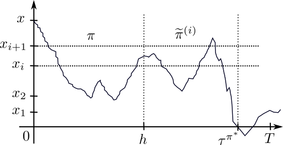
where and . Notice that, for we have that . In addition, in the case , we take the index such that , and follow the strategy , for . Figure 1 shows the graphical representation of the strategy . In addition, notice that if , then , for all , for and for . Therefore, we have that . Furthermore, on , by Equation (4.6) we obtain
| (4.8) |
Consenquently, similar to Equation (4.2) we have that
Now, we use the fact that
Therefore, using Equation (4.8), we get
| (4.9) |
Since is arbitrary, we obtain that , proving the theorem for .
We now consider the general case, when . Let be a partition of , where , . Define
Note that are simple functions such that , -a.s. Further, take only a finite number of values. Further, if and if , for all . Using the same argument as (4.2), it is easy to show that .
The reverse inequality shall prove utilizing induction on , in order to
| (4.10) |
For we have that on , so there is nothing to prove. Suppose that (4.10) holds for . We shall argue that (4.10) holds for as well. For any , on we have that and
Then, we have -a.s. on for all . Now, on we have
| (4.11) |
-a.s. on . Note that on the set , takes only values, then by inductional hypothesis and the Markov property of the process , we have that
| (4.12) |
Utilizing this inequality into (4.11) we obtain
| (4.13) |
-a.s. on . The las inequality is due to (4.1) for fixed time . Consequently, we obtain for all , whence for all . Finally, utilizing dominated convergence theorem, together with the continuity of the value function, we proof the general identity of (4.1). This complete the proof. ∎
5 The Hamilton-Jacobi-Bellman equation
We are now ready to calculate the Hamilton-Jacobi-Bellman (HJB) equation associated to our optimization problem (2.6). Given be a constant there exist a strategy and such that . Using Itô’s Lemma for a function of two variables and a similar argument as in Section 2.2 of Azcue and Muler [Azcue and Muler (2014)], we find
| (5.1) |
where , , and is the distribution function of claim size. By Theorem 4.1 we have that
| (5.2) |
In the before equation we can let tend to zero. Assuming that is twice continuously differentiable in and continuously differentiable in , and dividing by and letting we get
where . This inequality has to hold for all . Therefore, this motives the Hamilton-Jacobi-Bellman equation by our optimization problem
| (5.3) |
with the boundary conditions , and where is the following second order partial integro-differential operator
for , the set of all functions twice continuously differentiable in and continuously differentiable in .
In addition, by Lemma 1, is strictly increasing and concave in with the boundary condition . Because the left hand side of (5.3) is quadratic in , we find that
| (5.4) |
Strategy will be our candidate for the optimal strategy. As is the amount invested in the risky asset, we have that , where represent the proportion of the surplus invested in the risky asset at time (hence for all ). Then, using (5.4) we find that
| (5.5) |
Note that, if the expected return of the stock market is greater than the risk-free rate , then , but that does not guarantee that is less than 1. Thus, if the right strategy would be . In the other hand, if the right strategy will be .
Theorem 5.1.
Suppose that there exists a solution of (5.3) that is a function twice continuously differentiable in and continuously differentiable in with boundary conditions . Then . If
| (5.6) |
is bounded and for all , then and an optimal strategy is given by .
Proof.
Let and let be the interarrival times in . The controlled investment process has finite jumps on each finite time interval . The jump size of the process at time es denoted by , then
where is the claim size at time . Consider the process conditioned on . Using Itô’s Lemma for a jump process (see for details [Cont and Tankov (2004)]), we have that
It is known that the stochastic integral is a martingale. Thus
Then, by the Hamilton-Jacobi-Bellman equation (5.3) we have that
Because , we obtain the following inequality
Now, if we take supremum over all strategies , we have that .
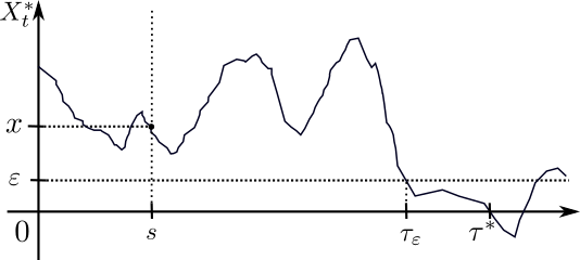
Suppose now that is bounded by a value . Note that by the Hamilton-Jacobi-Bellman equation (5.3), whenever , where is the process with optimal investment strategy . Choose and define . Note that converges monotonically as , where is the time to ruin of the process .
As is a concave function, we have that . Thus, is increasing on and for all . Then, is bounded on . Now, by the Hamilton-Jacobi-Bellman equation (5.3) and the Itô formula we obtain
| (5.7) |
In addition, as is bounded, then the second moment of is bounded for all , and . Thus, we have that is a martingale (for more details see [Karatzas and Shreve, 1991], [Ikeda and Watanabe, 1981]). Therefore, we obtain the following equation,
Notice that, as we have that
monotonically. The first term can be written as follow
The term is bounded by , which is uniformly bounded. Thus, by the boundary condition, it converges to . Again, by boundary condition, the second term converges monotonically to
This completes the proof. ∎
Finally, suppose that is a solution of (5.3) twice continuously differentiable in and continuously differentiable in with boundary conditions . Assume that there exists some constant such that
Remember that and . Then
Therefore, for some constants and we have that
This bound for the solution motivate trying a solution of the form .
6 Numerical example
We apply the method to the Cobb-Douglas type utility function , where , , in order to solve the optimization problem (2.6) trying a solution of the form for a continuously differentiable function with boundary condition . By (5.4) we have that the optimal strategy for our problem is given by
| (6.1) |
and the optimal proportion of the surplus invested in the risky asset at time is given by
| (6.2) |
Notice that in this case solving our optimization problem we obtain that the optimal proportion to be invested in the risky asset is the Merton ratio, introduced in [Merton R. (1969)]. Next, by the HJB equation (5.3) we obtain the following equation
Thus, the function satisfies the following relation
with boundary condition , where
for all and . Thus, we have that satisfies the differential equation
In order to solve these we are now going to use the substitution obtaining the differential equation , where . We thus find that the solution is given by
| (6.3) |
Exponential claim sizes: Assume that the claim sizes has distribution, i.e., . Then, we obtain the following identity
Thus, we have that as . Using this result is straightforward prove the following asymptotic result for the function .
Proposition 1.
Let be a sequence of independent, identically distributed (i.i.d). random variables having distribution. Then the following hold.
-
1.
If , then
where is the optimal proportion of the surplus invested in the risky asset.
-
2.
If , then .
6.1 Simulation of the ruin probability with and without optimal investment
In this section, we conduct Monte Carlo simulation in order to compute and compare the behavior of the ruin probability with and without optimal investment. For the purpose of comparison, ruin probability with and without optimal investment are calculated to Pareto and Weibull distribution as claim sizes. The ruin probability for the risk process with investment can be simulated by randomly drawing sample paths according to the process and counting the trajectories that lead to ruin and dividing this number by the total number of simulated trajectories. Thus, we get an unbiased estimator of the ruin probability
| (6.4) |
where is the set of all trajectories that lead to ruin up to time . Notice that to estimate the ruin probability it is necessary to simulate a sample trajectories of the jump-diffusion process
where is a compound Poisson process.
Now, we wish to simulate paths of the process without knowing its distribution or an explicit solution to the equation SDE in order to know if each simulated trajectory goes to ruin or not. We can simulate a discretized version of the jump-diffusion process. In particular, we simulate a discretized trajectories, where is the number of time steps, is a constant and . The smaller the value of , the closer our discretized path will be to the continuous-time path of that we wish to simulate (for more details see example [Karatzas and Shreve, 1991], [Oksendal (2000)] and [Ikeda and Watanabe, 1981]).
In the literature there are several discretization schemes available, the simplest approach is the Euler scheme. The Euler method is intuitive and easy to implement, and in our case we get the following discretize version
| (6.5) |
where the are i.i.d. .
Note that the risk process with investment has finite jumps on any finite interval , and in absence of claims (or between the jumps of ) is continuous and satisface the discretized version of the process
The jump size of the process at time is denoted by . The notation refers to . Thus, if the jump in the compound Poisson process occurs at time we have
where is the claim size at time .
Taking in account previous remarks, an approach to stimulating a discretized version of on the interval is given by
-
1.
First simulate the arrival times in the compound Poisson process up to time .
-
2.
Use a pure diffusion discretization between the jump times.
-
3.
At the arrival time , simulate the claim size conditional on the value of the discretized process, , immediately before .
We consider the case of a Weibull and Pareto distribution for the claim size (severity) with and , frequency parameter , premium rate and safety loading factor . Parameters to the optimal investment are: risk-free rate , expected return , volatility and risk aversion . In our simulation we have around of 0.48% monthly excess return and Merton ratio . The choice of the parameters is purely academic and year.
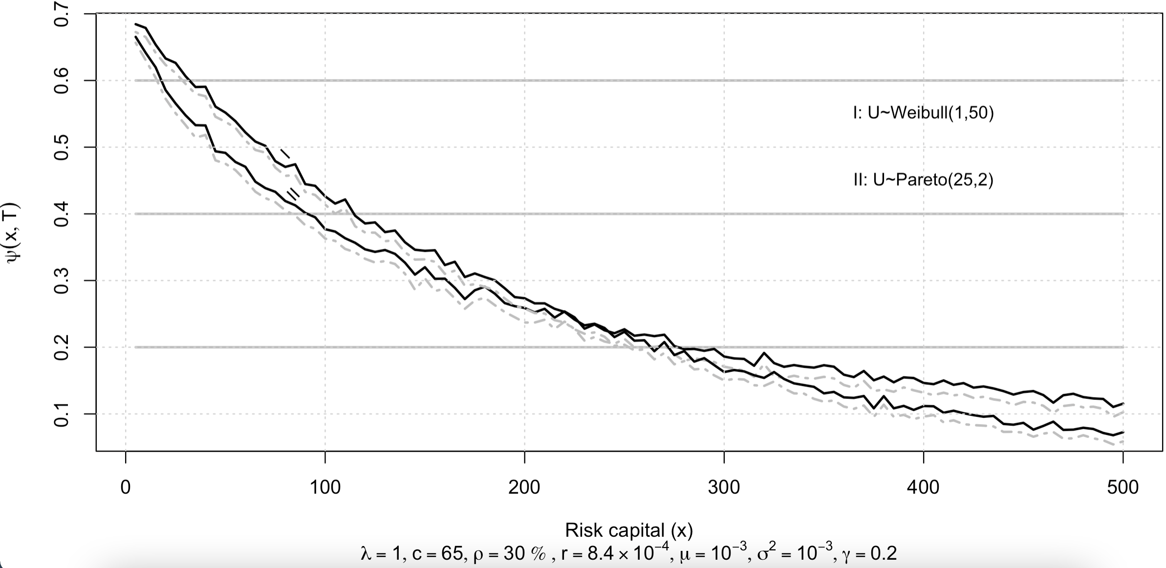
Using the discretized version of the process 6.5, we simulate trajectories for each case. Numerical results, in Figure 3, show that the optimal strategy in one year reduce the ruin probability of the portfolio for diferent claim size distributions. Solid line is the ruin probability without investment and dashed line is the ruin probability with investment. The difference in ruin probabilities seems to be small, but notice that, with Exponential claim size for capital risk we have a ruin probability of 0.4306 with optimal investment, while the ruin probability is 0.4406 without investment . In Table 1, we summarize our results for Exponential, Pareto and Weibull distributions for the claim size, and different values of risk capital .
| Exponential | Pareto | Weibull | ||||
|---|---|---|---|---|---|---|
| 100 | 0.4406 | 0.4372 | 0.377 | 0.3728 | 0.4262 | 0.424 |
| 200 | 0.274 | 0.2676 | 0.2588 | 0.247 | 0.2734 | 0.268 |
| 400 | 0.1014 | 0.097 | 0.1464 | 0.1418 | 0.1118 | 0.106 |
Acknowledgements.
I would like to thank Prof. A. Yambartsev for very valuable discussions and his encouragement. J.C.H would like to thank the CONCYTEC- FONDECYT, contract 232-2019 and 427-2019, for the financial support.
References
- [Andersen and Sparre (1957)] Andersen, E. Sparre. (1957). On the collective theory of risk in case of contagion between the claims. Transactions XVth International Congress of Actuaries, New York, II, 219-229.
- [Asmusen (1984)] Asmusen, S. Aproximations for the probability of ruin within finite time, Scand. Act. J. 31-57 (1984).
- [Asmusen (1989)] Asmussen, S. Risk theory in a markovian environment. Scand. Actuarial I., 66 - 100. (1989)
- [Asmusen and Albrecher (2010)] Asmusen, S. and Albrecher, H.: Ruin probabilities, World Scientific Publishing, Second Edition (2010)
- [Azcue and Muler (2014)] Azcue P. and Muler N.. Stochastic optimization in insurance: A dynamic programming approach Springer (2014).
- [Browne (1995)] Browne S. (1995). Optimal investment policies for a firm with a random risk process: exponential utility and minimizing the probability of ruin. Math. Oper. Res., 20(4), 937–958.
- [Cont and Tankov (2004)] Cont R. and Tankov P. . Financial Modelling with Jump Processes, Chapman & Hall / CRC Press (2004).
- [Cramer (1930)] Cramér, H. (1930). On the Mathematical Theory of Risk. Skandia Jubilee Volume, Stockholm.
- [Cramer (1945)] Cramér, H.: Collective Risk Theory. Skandia Jubilee Volume, Stockholm (1945)
- [De Finetti (1957)] De Finetti, B. (1957). Su un’ impostazione alternativa dell teoria collettiva del risichio. Transactions of the XVth congress of actuaries, (II), 433–443.
- [Diko et al. (2011)] Diko, P. and Usabel, M.: A numerical method for the expected penalty reward function in a Markov-modulated jump diffusion process. Insurance: Mathematical and Economics, V49, Issue 1, 126–131 (2011).
- [Embrechts and Veraverbeke (1982)] Embrechts, P. and Veraverbeke, N. Estimates for the probability of ruin with special emphasis on the possibility of large claims. Insurance: Mathematics and Economics 1, 55 - 72. (1982)
- [Embrechts et al. (1997)] Embrechts P., Kluppelberg C, and Mikosch T. Modelling Extremal Events for Insurance and Finance. Stochastic Modelling and Applied Probability. Springer (1997).
- [Gordon (1959)] Gordon,M.J. (1959). Dividends, earnings and stock prices, Review of Economics and Statistics, 41, 99–105.
- [Hipp and Plum (2000)] Hipp, C. and Plum, M. (2000) Optimal investment for insurers. Insurance: Mathematical and Economics, 27, 215–228.
- [Hipp and Plum (2003)] Hipp, C. and Plum, M. (2003). Optimal investment for investors with state dependent income, and for insurers. Finance and Stochastics, 7, 299–321 (2003).
- [Hipp and Vogt (2003)] Hipp C. and Vogt M. Optimal dynamic XL reinsurance. ASTIN Bull 33(2):193–207 (2003).
- [Hipp (2004)] Hipp, C.: Stochastic control with Application in Insurance. Stochastics Methods in Finance, pp. 127–164. Lecture notes in Mathematics, No 1856, Springer, Berlin (2004).
- [Ikeda and Watanabe, 1981] Ikeda N. and Watanabe, S. (1981). Stochastic Differential Equations and Diffusion processes. North Holland, Amsterdam.
- [Karatzas and Shreve, 1991] Karatzas I. and Shreve, S. (1991). Brawnian Motion and Stochastic Calculus. Springer.
- [Lundberg (1903)] Lundberg, F. (1903). I. Approximerad Framställning av Sannolikhets - funktionen. Almqvist-Wiksell, Uppsala.
- [Lundberg (1909)] Lundberg, F. (1909). Über Die Theorie Der Rückversicherung. Transactions of the VIth International Congress of Actuaries, vol. 1, pp. 877-948
- [Landsman and Sherris (2001)] Landsman, Z. and Sherris, M.: Risk measures and insurance premium principles. Insurance: Mathematics and Economics, 29(1), 103 - 115. (2001)
- [Merton R. (1969)] Merton Robert C. (1969). Lifetime Portfolio Selection under Uncertainty: The Continuous-Time Case. The Review of Economics and Statistics. 51, No. 3 , pp. 247–257
- [Merton R. (1971)] Merton Robert C. (1971). Optimum Consumption and Portfolio Rules in a Continuous-Time Model. Journal of Economic Theory. 3, pp. 373–413
- [Mikosh (2004)] Mikosh, T. Non-Life Insurance Mathematics: an introduction with Stochastic Processes. Springer (India), New Delhi (2004)
- [Modigliani1 and Miller (1961)] Miller, M. H. and Modigliani, F. (1961). Dividend policy, growth, and the valuation of shares, The Journal of Business, 34(4), 411–433.
- [Ramasubramanian (2009)] Ramasubramanian, S.: Lectures on Insurance Models, Hindustan Book Agency, India, New Delhi, (2009).
- [Rolski et al. (2005)] Rolski, T. , Schmidli, H., Schmidt, V. and Teugels, J.L.: Stochastic Processes for Insurance and Finance. 8th edition. Elsevier India, New Delhi, (2005).
- [Oksendal (2000)] Oksendal Bernt. Stochastic Differential Equations, An Introduction with Applications. Springer, (2000).
- [Schmidli (2008)] Schmidli H. Stochastic control in insurance. Springer, New York (2008).
- [Teugels and Sundt (2004)] Teugels, J.L. and Sundt B. : Encyclopedia of Actuarial Science, 3 Vols. Wiley, Chichester (2004).
- [Thorin (1971)] Thorin, O. Further remarks on the ruin problem in case the epochs of the claims form a renewal process. Skand. AktuarTidskr., 14 - 38 and 121 - 142. (1971)
- [Thorin (1974)] Thorin, O. On the asymptotic behavior of the ruin probability for an infinite period when the epochs of claims form a renewal process. Scand. Actuarial J., 81 - 99. (1974)
- [Thorin (1975)] Thorin, O. Stationarity aspects of the Sparre Andersen risk process and the corresponding ruin probabilities. Scand. Actuarial J., 87 - 98. (1975)
- [Wang and Dhaene (1998)] Wang, S. and Dhaene, J.: Comonotonicity, correlation order and premium principles. Insurance: Mathematics and Economics, 22(3), 235 - 242 (1998)
- [Wang et al. (1997)] Wang, S., Young, V.R. and Panjer, H.: Axiomatic characterization of insurance prices. Insurance: Mathematics and Economics, 21(2), 173 - 183 (1997)
- [Young (2006)] Young, V. R. Premium Principles. John Wiley and Sons, Ltd. (2006)