Extension of unimodular gravity and the cosmological constant

Abstract

A new way is proposed to cancel the cosmological constant. The proposal involves the metric determinant acting as a type of self-adjusting $q$-field without need of a fine-tuned chemical potential. Since the determinant of the metric now plays a role in the physics, the allowed coordinate transformations are restricted to those with unit Jacobian. This approach to the cosmological constant problem is, therefore, similar to the unimodular-gravity approach of the previous literature. The resulting cosmology has been studied and the obtained results show the natural cancellation of an initial cosmological constant if quantum-dissipative effects are included.

I Introduction

The cosmological constant problem, at the interface of gravitation and elementary particle physics, is certainly one of the most important problems of modern physics Weinberg1989 ; Carroll2001 . In a nutshell, the main cosmological constant problem is as follows (throughout, we use natural units with $c=1$ and $\hbar=1$). The electroweak standard model of elementary particles involves a vacuum energy density $\epsilon_{V}^{\text{\,(EWSM)}}$ of the order of $(100\;\text{GeV})^{4}\sim 10^{44}\;\text{eV}^{4}$. Moreover, this energy density can be expected to vary as the temperature $T$ of the Universe drops. How, then, can the Universe end up with a vacuum energy density $\Lambda^{\text{(observed)}}$ of order $10^{-11}\;\text{eV}^{4}$? There are 55 orders of magnitude to explain. See, in particular, Ref. Carroll2001 for further discussion of the astronomical observations.

We remark that the cosmological constant problem is about canceling all different contributions to the vacuum energy density appearing over the whole history of the Universe and not about canceling just one number. For this reason, some form of adjustment mechanism seems to be called for. A particular adjustment mechanism has been proposed that is inspired by condensed matter physics, where a special type of vacuum variable $q$ provides for the natural cancellation of any previously available vacuum energy density KlinkhamerVolovik2008a ; KlinkhamerVolovik2008b .

The 4-form realization of $q$-theory suggests the existence of a chemical potential $\mu$ which leads to the cancellation of the gravitating vacuum energy density in equilibrium. However, the dynamics towards the equilibrium remains a problem since the relaxation of $\mu$ to its equilibrium value $\mu_{0}$ in the Minkowski vacuum was not demonstrated in the original papers KlinkhamerVolovik2008a ; KlinkhamerVolovik2008b .

Here, we consider another version of $q$-theory, where the role of the dynamical vacuum variable $q$ is played by the tetrad determinant KlinkhamerVolovik2019 . The chemical potential in this case may arise, for example, from a model of the vacuum as a spacetime crystal, where the number of lattice points is conserved, which gives rise to a chemical potential $\mu$.

The present paper essentially consists of two parts, where the second part (Secs. VI and VII) presents the main cosmological results from an assumed action (18). This assumed action, with only the fields of general relativity and the standard model of elementary particles, has a single nonstandard term involving the square root of the negative metric determinant (or, equivalently, the tetrad determinant). The first part (Secs. II–V) gives a condensed-matter-inspired motivation for the assumed action (18), but this action may very well have another origin.

The specific content of the first part, which can be skipped in a first reading, is as follows. In Sec. II, we present a physical motivation for having a chemical potential associated with the metric determinant. In Sec. III, we then show that the metric determinant can, in principle, cancel an initial cosmological constant, but the chemical potential needs to be fine-tuned. In Sec. IV, we avoid this fine-tuning of the chemical potential by introducing a nonstandard coupling of the metric determinant to matter, provided the allowed coordinate transformations are restricted to those with unit Jacobian. In Sec. V, we compare the new metric-determinant cancellation mechanism with what happens in condensed matter physics, which was the inspiration of our previous work on $q$-theory (for a brief review, see App. A in Ref. KlinkhamerVolovik2022-BBasTopQPT ).

The specific content of the second part, which can essentially be read without knowledge of the first part, is as follows. In Sec. VI, we present a basic model for cosmology with the metric determinant as a dynamic variable. We have both analytic and numeric results, but the cosmological constant cannot be cancelled in general. For that cancellation, we may need to appeal to nonreversible effects such as dissipation. In Sec. VII, we consider a phenomenological model of cosmology with quantum-dissipative effects included. The main result is that it appears possible to cancel a cosmological constant for initial boundary conditions within a finite domain (attractor behavior). The three appendices give further results.

In Sec. VIII, we give some concluding remarks on both parts.

II Spacetime crystal: Conservation of lattice points

As explained in Sec. I, it is possible to skip ahead to Sec. VI in a first reading. The present section sets out to explore a potential condensed-matter-type origin of the action used later for cosmology.

For a $(3+1)$-dimensional vacuum crystal with elasticity tetrads NissinenVolovik2019 ; Nissinen2020

$$E^{\,a}_{\alpha}(x)=\partial_{\alpha}\,X^{a}(x)\,,$$ (1)

the density $n$ of lattice points is determined by the volume of the Brillouin zone,

$$n(x)=\frac{1}{(2\pi)^{4}}\,e^{\alpha\beta\gamma\delta}\,E^{\,0}_{\alpha}(x)\,E^{\,1}_{\beta}(x)\,E^{\,2}_{\gamma}(x)\,E^{\,3}_{\delta}(x)\,.$$ (2)

Neglecting factors of $2\pi$, the quantity $n(x)$ equals the tetrad determinant $E(x)$ with the dimension of inverse length to the fourth power (the phase fields $X^{a}$ are dimensionless).

As suggested in Sec. VII of Ref. NissinenVolovik2019 , it is, in principle, possible that gravity emerges from a vacuum crystal with elasticity tetrads (1). There would then be an effective metric $g_{\alpha\beta}$ built from the elasticity tetrads, $g_{\alpha\beta}\propto\eta_{ab}\,E^{\,a}_{\alpha}\,E^{\,b}_{\beta}\,$. In that case, we can identify the tetrad determinant with the square root of minus the metric determinant, $E\propto\sqrt{-g}$. If the vacuum crystal has a fundamental length scale $\ell\equiv 1/M$, we would have

$$M^{-4}\,n(x)\equiv M^{-4}\,E(x)=\sqrt{-g(x)}\,,$$ (3)

which relates the lattice-point density $n$ to the emergent dimensionless metric $g_{\alpha\beta}$ that enters the Einstein–Hilbert action for gravity.

The total number of lattice points is given by

$$N=\int d^{4}x\,n(x)\,,$$ (4)

and it is natural to assume that this number is conserved. Then there is a Lagrange multiplier in the action,

$$S_{N}=-\mu\,N=-\mu\int d^{4}x\;n(x)\,,$$ (5)

where $\mu$ is the corresponding chemical potential. This chemical potential $\mu$ is dimensionless, which may be of direct relevance for a recent proposal to replace the big bang singularity by a quantum phase transition KlinkhamerVolovik2022-BBasTopQPT .

Instead of a spacetime crystal with a conserved number of lattice points, one might consider the conventional vacuum, but now with conservation of the 4-volume. This would give the same action (5) with $n$ from (3), which is really the only input needed for the following.

III Cancellation of the cosmological constant

The total action is

$$S=S_{G}+S_{M}+S_{N}\,,$$ (6)

with the action $S_{N}$ from (5), the gravitational Einstein–Hilbert action $S_{G}$ containing the Ricci curvature scalar, and the action $S_{M}$ for the matter fields. The action (6) is fully diffeomorphism invariant.

To study the Minkowski vacuum, we can neglect the gradient terms in the matter action and also the curvature term. The matter term then depends only on a potential $\epsilon\,$:

$$S_{M}=\int d^{4}x\,M^{-4}\,n\,\epsilon(\Phi)\,,$$ (7)

where $\Phi$ is a generic scalar field, considered here to be without gradients, i.e., constant over the spacetime manifold. The equilibrium vacuum state is obtained by variation of this last action over $\Phi$:

$$\left.\frac{d\epsilon(\Phi)}{d\Phi}\right|_{\Phi=\Phi_{0}}=0\,.$$ (8)

The equilibrium value $\Phi_{0}$ gives the vacuum energy contribution $\epsilon(\Phi_{0})$ to the effective cosmological constant. It is nonzero if there is no artificial fine-tuning.

The total contribution to the vacuum energy density $\rho_{\text{vac}}$ that enters the Einstein gravitational field equation comes from $S_{M}+S_{N}$ by variation of $M^{-4}\,n$,

$$\rho_{\text{vac}}=\epsilon(\Phi_{0})-\mu\,M^{4}\,.$$ (9)

From the Einstein equation applied to the state with zero curvature $R=0$ and zero temperature $T=0$, we obtain the equilibrium value $\mu=\mu_{0}$ of the Minkowski vacuum,

$$\rho_{\text{vac}}=\epsilon(\Phi_{0})-\mu_{0}\,M^{4}=0\,.$$ (10)

The vacuum energy density of the matter field $\epsilon(\Phi_{0})$ is naturally cancelled by the chemical potential $\mu=\mu_{0}$. This is similar to the 4-form $q$-theory KlinkhamerVolovik2008a , where the equations $\epsilon(q)-\mu\,q=0$ and $d\epsilon/dq-\mu=0$ determine both $q_{0}$ and $\mu_{0}$.

The main problem, now, is in the dynamics: how to describe the dynamical relaxation of the parameter $\mu$ to its equilibrium value $\mu_{0}$.

IV Metric determinant as a dynamic variable

Probably the best way to deal with the chemical-potential fine-tuning problem is to introduce the dependence of the matter energy density on $n$, i.e, to have a potential $\epsilon=\epsilon(\Phi,\,n)$. In this case, the action is invariant only under those coordinate transformations that have a Jacobian equal to unity,

$$\det\Big{(}\partial x^{\prime\,\alpha}/\partial x^{\beta}\Big{)}=1\,.$$ (11)

These restricted coordinate transformations also appear in the unimodular-gravity approach to the cosmological constant problem Einstein1919 ; vanderBij-etal1982 ; Zee1983 ; BuchmuellerDragon1988 ; HenneauxTeitelboim1989 (a brief review is given in Sec. VII of Ref. Weinberg1989 ).

The Minkowski vacuum may then have a continuous set of $\mu$ values, which determine the equilibrium values $n_{0}(\mu)$ of the metric determinant in equilibrium. In other words, there are many different quantum vacua in flat Minkowski spacetime and they are parametrized by the values $\mu$ of the chemical potential. (Recall that the Minkowski vacuum in the original $q$-theory KlinkhamerVolovik2008a has a single value $\mu_{0}$ for the chemical potential.)

The Einstein gravitational field equation (to be given explicitly in Sec. VI.1) now contains the following vacuum energy density:

$$\rho_{\text{vac}}(\Phi,n)=M^{4}\,\frac{d}{dn}\Big{[}n\,M^{-4}\,\epsilon(\Phi,\,n)-\mu\,n\Big{]}=\epsilon(\Phi,\,n)+n\,\frac{d\epsilon(\Phi,\,n)}{dn}-\mu\,M^{4}\,.$$ (12)

The equilibrium vacua are obtained by variation of the action over both $\Phi$ and $n$,

$$\frac{d\epsilon(\Phi,\,n)}{d\Phi} = 0\,,$$ (13a)

$$\rho_{\text{vac}}(\Phi,n) = 0\,.$$ (13b)

These equations determine the equilibrium values of the variables $\Phi$ and $n$ as functions of $\mu$, that is, having $\Phi=\Phi(\mu)$ and $n=n(\mu)$ over a finite range of $\mu$. This range does not necessarily include $\mu=0$, as can be seen from the example below. Hence, it is necessary to introduce $\mu$ and we cannot just forget about it.

The simplest example is

$$\epsilon(\Phi,\,n) = \widetilde{\epsilon}(\Phi)\left(1+\frac{n}{n_{\text{scale}}}\right)\,,$$ (14a)

with a fixed positive density $$n_{\text{scale}} M^{4}$$ (alternatively written as ). The corresponding gravitating vacuum energy density from (12) reads

$$\rho_{\text{vac}}(\Phi,n) = \widetilde{\epsilon}(\Phi)\left(1+2\,\frac{n}{n_{\text{scale}}}\right)-\mu\,M^{4}\,.$$ (14b)

Now, condition (13a) gives the equilibrium value $\Phi_{0}$ of the matter field $\Phi$ and condition (13b) gives the equilibrium value $n_{0}=n_{0}(\mu)$ of the metric determinant $n\propto\sqrt{-g}$,

$$n_{0}(\mu)=n_{\text{scale}}\;\frac{\mu\,M^{4}-\widetilde{\epsilon}(\Phi_{0})}{2\,\widetilde{\epsilon}(\Phi_{0})}\,.$$ (15)

Assume, for definiteness, that $\widetilde{\epsilon}(\Phi_{0})>0$. Then, self-sustained Minkowski vacua with $n_{0}>0$ exist only at $\mu\,M^{4}>\widetilde{\epsilon}(\Phi_{0})$, which does not allow for $\mu=0$ as mentioned above. [Incidentally, the condition $\mu\,M^{4}>\widetilde{\epsilon}(\Phi_{0})$ can be relaxed by modifying the $\epsilon(\Phi,\,n)$ Ansatz (14a); a related example will be presented in the last paragraph of App. A.]

This approach with a dynamically-fixed metric determinant is an extension of the unimodular-gravity approach Einstein1919 ; vanderBij-etal1982 ; Zee1983 ; BuchmuellerDragon1988 ; HenneauxTeitelboim1989 , where typically the metric determinant is eliminated as a dynamical variable; see, e.g., the second and third paragraphs of Sec. VII in Ref. Weinberg1989 . (Some related ideas on a dynamical measure of integration in the action, generalizing $\sqrt{-g}$, appear in Ref. BensityGuendelman-etal2020 and references therein.)

The simple model (14) can be used for calculations of the dynamics of the cosmological constant, since, contrary to the original $q$-theory, the relaxation to the Minkowski vacuum does not require the fine-tuning of $\mu$ to the value $\mu_{0}$. Instead of the problematic relaxation of $\mu$, there is the relaxation of $n$ at a given value $\mu\,M^{4}>\widetilde{\epsilon}(\Phi_{0})>0$ for the example considered.

We can also study the relaxation after a cosmological phase transition, at which the $\Phi_{0}$ value may change. Different from the original $q$-theory approach, this does not require a change in the chemical potential. After the transition, the quantity $n_{0}$ will be adjusted to a new equilibrium state, while $\mu$ remains fixed. Moreover, we can expect a phase transition between the self-sustained Minkowski vacuum with $\widetilde{\epsilon}(\Phi_{0})<\mu\,M^{4}$ and the state with $\widetilde{\epsilon}(\Phi_{0})>\mu\,M^{4}$, which can be expanding or contracting.

V Comparison with condensed matter physics

In condensed matter physics with conservation of particle number, there is the thermodynamic equilibrium equation,

$$\frac{d\epsilon}{dn}=\mu\,,$$ (16a)

and the Gibbs–Duhem relation at temperature $$T=0$$,

$$\rho_{\text{vac}}=\epsilon(n)-\mu\,n=-P\,.$$ (16b)

The combination of both relations determines $\mu$ and $n$ as a function of the pressure $P$.

If there is no external pressure, $P_{\text{external}}=0$, one obtains the nullification of the effective cosmological constant,

$$\rho_{\text{vac}}=\epsilon(n)-\mu\,n=-P=-P_{\text{external}}=0\,.$$ (17)

Here, the nullification of the vacuum energy is provided by the absence of an external environment. But only self-sustained systems can exist in the absence of external pressure.

For the example (14), self-sustained vacua exist if $\mu\,M^{4}>\epsilon(\Phi_{0})$. The vacua with $\mu\,M^{4}<\epsilon(\Phi_{0})$ are not self-sustained, so that the cosmological constant (the analog of the external pressure) is nonzero and leads to expansion or contraction of these vacua (a de-Sitter-type universe).

VI Cosmology: Basic model

VI.1 Action and Ansätze

We will now investigate the application to cosmology of the theory as discussed in the previous sections. These previous sections can, however, be skipped in a first reading, as the present section and the next are self-contained. Here, we aim to establish the asymptotic vanishing of the total gravitating vacuum energy density. For that, we simplify the theory to the bare minimum: we remove the scalar $\Phi$ field (which is not really needed for the cosmological-constant cancellation) and add a standard real scalar $X$ (needed to get the appropriate expansion of the Friedmann–Robertson–Walker-type model).

The postulated action is given by

$$S = S_{G}+S_{M}+S_{\Lambda-\text{plus}}+S_{N}\,,$$ (18a)

$$S_{G} = \int d^{4}x\,\sqrt{-g}\;\frac{R}{16\pi G_{N}}\,,$$ (18b)

$$S_{M} = \int d^{4}x\,\sqrt{-g}\;\left[\frac{1}{2}\,g^{\alpha\beta}\,\partial_{\alpha}X\,\partial_{\beta}X+\overline{\epsilon}(X)\right]\,,$$ (18c)

$$S_{\Lambda-\text{plus}} = \int d^{4}x\,\sqrt{-g}\;\epsilon(\Lambda,\,n)\,,$$ (18d)

$$S_{N} = -\mu\,\int d^{4}x\;n(x)\,,$$ (18e)

$$n(x) = \sqrt{-g(x)}\;M^{4}\,,$$ (18f)

where $g(x)$ is the determinant of the metric $g_{\alpha\beta}(x)$ with Lorentzian signature and $1/M$ is a fundamental length scale of the underlying theory. In (18c) and (18d), we simply take

$$\overline{\epsilon}(X) = \frac{1}{2}\,g_{2}\,M^{2}\,X^{2}\,,$$ (19a)

$$\epsilon(\Lambda,\,n) = \Lambda+\zeta\,n\,,$$ (19b)

with real parameters $g_{2}\geq 0$ and $\zeta>0$. We emphasize that, strictly speaking, the only new input is the single term $n\propto\sqrt{-g}$ in the potential (19b), consistent with having coordinate invariance restricted by (11). A possible condensed-matter-type origin of the action (18) has been discussed in Secs. II–V, but this action can also have an entirely different origin.

In the resulting gravitational field equation,

$$\frac{1}{8\pi G_{N}}\left(R_{\alpha\beta}-\frac{1}{2}\,R\,g_{\alpha\beta}\right)=\rho_{\text{vac}}\,g_{\alpha\beta}+T^{M}_{\alpha\beta}\,,$$ (20)

we have

$$\rho_{\text{vac}} = \Lambda+2\,\zeta\,n-\mu\,M^{4}\,,$$ (21a)

$$\Lambda = \lambda\,M^{4}\,,$$ (21b)

where the chemical potential $\mu\neq 0$ traces back to the action term (18e) and $n$ has been defined by (18f). Taking the covariant divergence of (20) and using the contracted Bianchi identities, we obtain the following combined energy-momentum conservation relation:

$$\Big{(}\rho_{\text{vac}}\,g_{\alpha\beta}+T^{M}_{\alpha\beta}\Big{)}^{;\,\beta}=0\,,$$ (22)

where the semicolon stands for a covariant partial derivative (the colon stands for a standard partial derivative). If the matter component is separately conserved, $\left(T^{M}_{\alpha\beta}\right)^{;\,\beta}=0$, then equally so for the vacuum component, so that $\rho_{\text{vac}}^{\hskip 11.38109pt,\,\beta}=0$.

With diffeomorphisms restricted to those of unit Jacobian, the appropriate spatially-flat Robertson–Walker (RW) metric has been given in Ref. AlvarezFaedo2007 (see also Ref. Zee1983 ):

$$ds^{2} = g_{\alpha\beta}(x)\,dx^{\alpha}\,dx^{\beta}=-\widetilde{A}(t)\;dt^{2}+\widetilde{R}^{\,2}(t)\;\delta_{ij}\,dx^{i}\,dx^{j}\,,$$ (23)

where $t$ is the cosmic time coordinate from $x^{0}=c\,t=t$ and $\widetilde{A}(t)>0$ is an additional Ansatz function. The spatial indices $i$, $j$ in (23) run over $\{1,\,2,\,3\}$ and $\widetilde{R}(t)$ is the cosmic scale factor [the tilde marks the difference with the Ricci scalar appearing in (18b)]. For $\widetilde{A}(t)=\text{const}>0$, we recover the standard spatially-flat RW metric. We remark that the extended RW metric (23) gives the vacuum variable

$$n\propto\sqrt{-g}=(\widetilde{A}\,)^{1/2}\>|\widetilde{R}\,|^{3}\,,$$ (24)

with proportionality constant $M^{4}$ according to (18f).

If the scalar field $X$ is spatially homogeneous in the cosmological spacetime (23), $X=X(t)$, then its energy-momentum tensor corresponds to that of a perfect fluid with the following energy density and pressure Mukhanov2005 :

$$\rho_{X}(t) = \frac{1}{2}\,\frac{1}{a(t)}\,\left(\frac{dX(t)}{dt}\right)^{2}+\frac{1}{2}\,g_{2}\,M^{2}\,\Big{(}X(t)\Big{)}^{2}\,,$$ (25a)

$$P_{X}(t) = \frac{1}{2}\,\frac{1}{a(t)}\,\left(\frac{dX(t)}{dt}\right)^{2}-\frac{1}{2}\,g_{2}\,M^{2}\,\Big{(}X(t)\Big{)}^{2}\,.$$ (25b)

If the scalar field $$X X(t)=X_{0}\,\cos(\omega\,t)$$ is, moreover, rapidly oscillating, , then the time averages of the energy density and the pressure give the following matter equation-of-state parameter:

$$w_{M} = \frac{\langle P_{X}\rangle}{\langle\rho_{X}\rangle}=\frac{\omega^{2}/a-g_{2}\,M^{2}}{\omega^{2}/a+g_{2}\,M^{2}}\,,$$ (25c)

where the cosmological time scale relevant to $a(t)$ is assumed to be much larger than $1/\omega$ or $1/M$. Obviously, $g_{2}=0$ gives $w_{M}=1$ and a value $w_{M}=1/3$ follows from $\omega^{2}/a=2\,g_{2}\,M^{2}$.

In the following, we will work with this perfect fluid instead of the original scalar $X$ field and take $w_{M}=1/3$, which can be interpreted as a gas of ultrarelativistic particles.

VI.2 Dimensionless ordinary differential equations

Henceforth, we set

$$M=E_{\text{Planck}}\equiv 1/\sqrt{G_{N}}\,,$$ (26)

and introduce the following dimensionless quantities (the chemical potential $\mu$ is already dimensionless):

$$t \to\tau\,, \rho_{X}(t) \to r_{\chi}(\tau)\,, \widetilde{A}(t) \to a(\tau)\,,$$ (27a)

$$X(t) \to\chi(\tau)\,, P_{X}(t) \to p_{\chi}(\tau)\,, \widetilde{R}(t) \to r(\tau)\,,$$ (27b)

$$n(t) \to n(\tau)\,, \Lambda \to\lambda\,,$$ (27c)

where $n(\tau)$ is dimensionless and equal to $\sqrt{-g(\tau)}=\sqrt{a(\tau)}\,|r(\tau)|^{3}$.

From the field equations of the action (18) and using the homogeneous perfect fluid from the $\chi$ scalar, we obtain the following dimensionless ordinary differential equations (ODEs):

$$\dot{r}_{\chi}+3\,(1+w_{M})\,\left(\frac{\dot{r}}{r}\right)\,r_{\chi}=0\,,$$ (28d)

$$3\,\left(\frac{\dot{r}}{r}\right)^{2}=8\,\pi\,a\,\Big{(}r_{\chi}+r_{\text{vac}}\Big{)}\,,$$

$$\frac{2\,\ddot{r}}{r}+\left(\frac{\dot{r}}{r}\right)^{2}-\left(\frac{\dot{a}}{a}\right)\,\left(\frac{\dot{r}}{r}\right)=-8\,\pi\,a\,\Big{(}w_{M}\,r_{\chi}-r_{\text{vac}}\Big{)}\,,$$

$$r_{\text{vac}}=\lambda+2\,\zeta\,\sqrt{a}\,|r|^{3}-\mu\,,$$

where the overdot stands for differentiation with respect to $\tau$. These ODEs have three real parameters: the matter equation-of-state parameter $w_{M}>-1$ and two parameters entering the vacuum energy density $r_{\text{vac}}$, namely $\zeta>0$ and $\mu\neq 0$. Incidentally, the function $a(\tau)$ has been assumed to be positive, so that there is no difficulty in taking its square root.

It can be shown that the ODEs (28) give an equation for the constancy of the vacuum energy density,

$$\dot{r}_{\text{vac}}=0\,.$$ (29)

This equation corresponds to the energy-conservation equation of a homogeneous perfect fluid with equation-of-state parameter $w_{\text{vac}}=-1$, compared with (28d) for the matter component. In fact, (29) traces back to (22) for matter with $\left(T^{M}_{\alpha\beta}\right)^{;\,\beta}=0$, so that $\rho_{\text{vac}}^{\hskip 11.38109pt,\,\beta}=0$. In Sec. VII, we will introduce a vacuum-matter energy exchange, but here we do without and keep (29).

VI.3 Analytic Friedmann-type solution for $\mathbf{w_{M}=1/3}$

We now present an exact solution of the ODEs (28) for $w_{M}=1/3$ (an exact solution for general $w_{M}>-1$ is given in App. A). We take the following Ansatz functions for $\tau>0$:

$$a(\tau) = \alpha\;\tau^{-2\,p}\,,$$ (30a)

$$r(\tau) = \alpha^{-1/6}\;\widehat{r}\;\tau^{p/3}\,,$$ (30b)

$$r_{\chi}(\tau) = \alpha^{-1}\;\widehat{\chi}\;\tau^{-m}\,,$$ (30c)

with positive parameters $\alpha$, $p$, $\widehat{r}$, $\widehat{\chi}$, and $m$. The vanishing of $r_{\text{vac}}$ from (28d) gives immediately

$$\widehat{r}_{\text{\,sol}}=\sqrt[3]{\frac{\,1}{2\,\zeta}\;\big{(}\mu-\lambda\big{)}}\,,$$ (31)

where, for a given value $\mu>0$, the dimensionless cosmological constant $\lambda$ must obey the following condition:

$$\lambda<\mu\,,$$ (32)

so that $\lambda$ can also be negative. Here, and in the following, we have assumed a positive $\mu$, but similar results are obtained for a negative $\mu$.

For the Ansatz functions (30), the dimensionless Ricci and Kretschmann curvature scalars read

$$\mathcal{R} = \frac{2}{3}\,p\,\big{(}5\,p-3\big{)}\,\frac{1}{\alpha}\,{\tau}^{-2\,(1-p)}\,,$$ (33a)

$$\mathcal{K} = \frac{4}{27}\,p^{2}\,\big{(}9-24\,p+17\,p^{2}\big{)}\,\frac{1}{\alpha^{2}}\,{\tau}^{-4\,(1-p)}\,.$$ (33b)

Restricting the power $p$ of the Ansatz functions to the range

$$0<p<1\,,$$ (34)

we look for an expanding ($p>0$) Friedmann-type universe approaching Minkowski spacetime (different from a de-Sitter spacetime at $p=1$; cf. Eq. (52) in Ref. Bamba-etal2016 ). Some details of the analytic de-Sitter-type solution with $p=1$ and $\widehat{\chi}=0$ are given in App. B.

With the Ansatz functions (30), the three ODEs from (28) reduce to the following expressions:

$$0 = \frac{1}{\alpha}\,\left(4\,p/3-m\right)\,\widehat{\chi}\,{\tau}^{-1-m}\,,$$ (35a)

$$0 = \frac{p^{2}}{3\,{\tau}^{2}}-8\,\pi\,\widehat{\chi}\,{\tau}^{-m-2\,p}\,,$$ (35b)

$$0 = \frac{p^{2}}{{\tau}^{2}}-\frac{2\,p}{3\,{\tau}^{2}}+\frac{8}{3}\,\pi\,\widehat{\chi}\,{\tau}^{-m-2\,p}\,.$$ (35c)

These equations have an exact solution,

$$p_{\text{\,sol}} = 3/5\,,$$ (36a)

$$m_{\text{\,sol}} = 4/5\,,$$ (36b)

$$\widehat{\chi}_{\text{\,sol}} = \frac{3}{200\,\pi}\approx 0.00477465\,,$$ (36c)

for arbitrary $\alpha>0$. Technically speaking, the solution exists because of an interplay between the two metric Ansatz functions and the matter energy density. The evaluated matter equation (35a) fixes the power $m$ to be equal to $4\,p/3$. The evaluated first Friedmann equation (35b) then fixes $p=3/5$ and $m=4/5$, so that both terms in the equation get the same temporal dependence $\tau^{-2}$ and cancel each other for an appropriate value of the constant $\widehat{\chi}$. It turns out that the evaluated second Friedmann equation (35c) is then also satisfied.

The main points of this cosmology are

• an expanding Friedmann-type universe with cosmic scale factor $r\sim\tau^{1/5}$.

• a decreasing perfect-fluid energy density and pressure $r_{\chi}(\tau)=3\,p_{\chi}(\tau)\sim\tau^{-4/5}$.

• a cosmological constant cancelled by $\sqrt{-g}=\widehat{r}_{\text{\,sol}}$ from (31), provided condition (32) holds, so that $r_{\text{vac}}(\tau)=0$.

• the curvature scalars $\mathcal{R}(\tau)\sim 0$ and $\mathcal{K}(\tau)\sim\tau^{-8/5}$, approaching Minkowski spacetime for $\tau\to\infty$.

Observe that, for a given value $\mu$, we have a whole family of asymptotic solutions depending on the cosmological constant $\lambda$ via (31), as long as condition (32) holds. The numerics must tell us whether or not there is an attractor behavior towards Minkowski spacetime.

VI.4 Initial boundary conditions

Before we turn to the numerical evaluation of the ODEs (28), we need to address the delicate issue of boundary conditions. We are concerned with three functions: $a(\tau)$, $r(\tau)$, and $r_{\chi}(\tau)$. The corresponding function space is vast and we will seek guidance from the analytic solution obtained in Sec. VI.3.

So, we will start out at an arbitrary coordinate time $\tau_{\text{bcs}}>0$ and obtain boundary conditions on the three functions by considering small perturbations of the analytic solution as given by (30), (31), and (36), for $\alpha=1$. There are two kinds of perturbations, those that do not change $r_{\text{vac}}(\tau_{\text{bcs}})=0$ to leading order and those that do (let us call the first kind “mild” and the second kind “dangerous”). We have two types of perturbations in the first category [keeping $r_{\text{vac}}(\tau_{\text{bcs}})\approx 0$] and one type of perturbations in the second category [making $r_{\text{vac}}(\tau_{\text{bcs}})$ nonzero to leading order in the perturbation].

The first type of “mild” perturbations can be written as follows:

$$\left\{\frac{\delta a}{a},\,\frac{\delta r}{r},\,\frac{\delta r_{\chi}}{r_{\chi}}\right\}^{(\text{type-}1)} = \left\{0,\,0,\,\delta_{1}\right\}\,,$$ (37a)

with a negative or positive infinitesimal $$\delta_{1}$$. For this type-1 perturbation, the vacuum energy density (28d) stays strictly zero.

The second type of “mild” perturbations has

$$\left\{\frac{\delta a}{a},\,\frac{\delta r}{r},\,\frac{\delta r_{\chi}}{r_{\chi}}\right\}^{(\text{type-}2)} = \left\{-\,6\>\delta_{2},\,\delta_{2},\,0\right\}\,,$$ (37b)

with a negative or positive infinitesimal $\delta_{2}$. The actual ratio of $\delta r/r$ and $\delta a/a$ in (37b) keeps the combination $\sqrt{a}\,|r|^{3}$ unchanged to first order in $\delta_{2}$ and precisely this combination enters the vacuum energy density (28d).

The third type of perturbations is in the “dangerous” category, having $r_{\text{vac}}\neq 0$ at the starting value $\tau=\tau_{\text{bcs}}\,$,

$$\left\{\frac{\delta a}{a},\,\frac{\delta r}{r},\,\frac{\delta r_{\chi}}{r_{\chi}}\right\}^{(\text{type-}3)} = \left\{\delta_{3}/6,\,\delta_{3},\,0\right\}\,,$$ (37c)

with a negative or positive infinitesimal $\delta_{3}$. These perturbations give, indeed, $r_{\text{vac}}\propto\delta_{3}$, which can be negative or positive.

Note, finally, that the above three perturbations are mutually orthogonal.

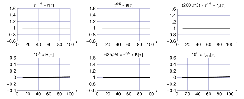
Figure 1: Numerical solution of the ODEs (28) with parameters $w_{M}=1/3$, $\zeta=1$, $\mu=3$, and $\lambda=1$. The initial boundary conditions are taken from the analytic solution (30), (31), and (36), for $\alpha=1$. Specifically, the boundary conditions at $\tau=\tau_{\text{bcs}}=10$ are: $\{a,r,\dot{r},r_{\chi}\}$ $=$ $\{0.0630957344,1.58489319,0.0316978638,0.000756730758\}$, where the $\dot{r}$ value has been obtained from the first Friedman equation (28d). The top row shows the three basic variables: the metric functions $r(\tau)$ and $a(\tau)$ and the dimensionless matter energy density $r_{\chi}$. The bottom row shows three derived quantities: the dimensionless Ricci curvature scalar $\mathcal{R}$, the dimensionless Kretschmann curvature scalar $\mathcal{K}$, and the dimensionless gravitating vacuum energy density $r_{\text{vac}}$ from (28d).

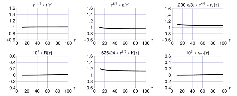
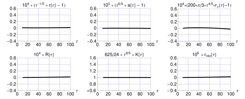
Figure 2: The model parameters and boundary conditions at $\tau=\tau_{\text{bcs}}=10$ are as in Fig. 1, but now with a type-1 perturbation (37a) for a constant $\delta_{1}=+1/10$: $\{a,r,\dot{r},r_{\chi}\}$ $=$ $\{0.0630957344,1.58489319,0.0332450001,0.000832403833\}$, where the $\dot{r}$ value has been obtained from the first Friedman equation (28d). Similar results are obtained for $\delta_{1}=-1/10$.

Figure 3: The model parameters and boundary conditions at $\tau=\tau_{\text{bcs}}=10$ are as in Fig. 1, but now with a type-2 perturbation (37b) for a constant $\delta_{2}=+10^{-6}$: $\{a,r,\dot{r},r_{\chi}\}$ $=$ $\{0.0630953559,1.58489478,0.0316978000,0.000756730758\}$, where the $\dot{r}$ value has been obtained from the first Friedman equation (28d). Similar results are obtained for $\delta_{2}=-10^{-6}$.

VI.5 Numerical results

The ODEs (28) can be solved numerically. Specifically, we use the first-order ODE (28d) and the second-order ODE (28d), together with the $\tau$ derivative of the first-order ODE (28d), while fixing the boundary conditions to satisfy (28d) as a constraint.

Numerical results for $\mu=3$ and $\lambda=1$ are shown in Fig. 1 for boundary conditions from the analytic solution of Sec. VI.3. The numerical solution of Fig. 1 essentially reproduces the analytic solution, which allows us to test the numerical accuracy. In fact, we see a small error building up in the dimensionless Ricci curvature scalar $\mathcal{R}(\tau)$, but the gravitating vacuum energy density $r_{\text{vac}}(\tau)$ stays close to zero within an accuracy of $10^{-7}$.

Further numerical results are shown in Fig. 3 for boundary conditions from a type-1 perturbation (37a). The other “mild” perturbation (37b) gives the numerical results shown in Fig. 3. The numerical solution of Fig. 3 asymptotically approaches the analytic solution from Sec. VI.3 for an $\alpha$ value approximately equal to $0.95$. The numerical solution of Fig. 3 also gets close to the analytic solution but not perfectly so, as $r_{\text{vac}}(\tau)$ is not exactly zero (the linear term in $\delta_{2}$ vanishes at $\tau=\tau_{\text{bcs}}$ but not the quadratic term).

For these five different boundary conditions (unperturbed, type-1 perturbations with $\delta_{1}=\pm 1/10$, and type-2 perturbations with $\delta_{2}=\pm 10^{-6}$), the vacuum energy density is found to be cancelled to high precision (less than $10^{-7}$ for the numerical solutions shown, where $\lambda=1$ sets the scale). Obviously, these “mild” type-1 and type-2 perturbations have $r_{\text{vac}}\approx 0$ at the starting value $\tau=\tau_{\text{bcs}}$, which is then not changed by the later dynamics [numerically, a nontrivial result; analytically, we have $\dot{r}_{\text{vac}}=0$, as discussed in Sec. VI.2].

As mentioned in Sec. VI.4, “dangerous” perturbations have $r_{\text{vac}}\neq 0$ at the starting value $\tau=\tau_{\text{bcs}}$. We have obtained numerical results for a type-3 perturbation (37c) with $\delta_{3}=+10^{-6}$, giving a constant vacuum energy density $r_{\text{vac}}=6.17444\times 10^{-6}$ (a related figure will be given in Sec. VII.3). Apparently, we need to modify the dynamics, in order to cure the “dangerous” perturbations. For this reason, modified ODEs with vacuum-matter energy exchange (earlier work Klinkhamer2017 already suggested the need for this type of energy exchange) will be introduced in the next section.

VII Cosmology: Quantum-dissipative effects

VII.1 Preliminary remarks

A general discussion of relaxation effects in $q$-theory has been presented in Ref. KlinkhamerSavelainenVolovik2016 . A specific calculation, for a standard spatially-flat Robertson–Walker metric [i.e., $\widetilde{A}(t)=1$ in (23)], relies on particle production by spacetime curvature ZeldovichStarobinsky1977 . The resulting Zeldovich–Starobinsky-type source term reads KlinkhamerVolovik-MPLA-2016

$$\Gamma_{\text{particle-production}}=\widehat{\gamma}\,\left|\widetilde{R}^{-1}\;\frac{d\widetilde{R}}{dt}\right|\,R^{2}\,,$$ (38)

with the cosmic scaling function $\widetilde{R}(t)$ of the metric (23) and the Ricci curvature scalar $R(t)=R\big{[}\widetilde{A}(t),\,\widetilde{R}(t)\,\big{]}$.

We then have for the cosmic evolution of the matter and vacuum energy densities:

$$\frac{d\rho_{M}}{dt}+\cdots = +\Gamma_{\text{particle-production}}\,,$$ (39a)

$$\frac{d\rho_{V}}{dt}+\cdots = -\Gamma_{\text{particle-production}}\,,$$ (39b)

because of energy conservation (22). Observe that Eqs. (39a) and (39b) are time-reversal noninvariant for the source term as given by (38). This time-reversal noninvariance is, of course, to be expected for a dissipative effect, in fact a quantum-dissipative effect as particle creation or annihilation is a genuine quantum phenomenon.

VII.2 Modified ODEs with vacuum-matter energy exchange

We now consider a relativistic matter component with equation-of-state parameter $w_{M}\equiv P_{\chi}/\rho_{\chi}=1/3$ and add a positive source term $\Gamma$ on the right-hand side of (28d). We then need to determine how this addition feeds into the other ODEs. Specifically, we take three steps towards modified ODEs with a phenomenological implementation of quantum-dissipative effects. Henceforth, we use the dimensionless variables from (27).

In step 1, we add a source term $\Gamma$ to the right-hand side of (28d) for $w_{M}=1/3$ to get

$$\dot{r}_{\chi}+4\,\left(\frac{\dot{r}}{r}\right)\,r_{\chi}=\Gamma\,.$$ (40a)

Next, we see how the new term in (40a) feeds into the two ODEs (28d) and (28d).

In step 2, we eliminate $r_{\chi}$ by taking the sum of one third of (28d) and (28d) for $w_{M}=1/3$,

$$\frac{1}{8\,\pi\,a}\,\left[\frac{2\,\ddot{r}}{r}+2\,\left(\frac{\dot{r}}{r}\right)^{2}-\left(\frac{\dot{r}}{r}\right)\,\left(\frac{\dot{a}}{a}\right)\right]=\frac{4}{3}\,r_{\text{vac}}\,,$$ (40b)

where the $r_{\text{vac}}$ expression will be recalled shortly.

In step 3, we take the derivative of (28d), use (40a) to eliminate $\dot{r}_{\chi}$, use (28d) to eliminate $r_{\chi}$, use the $\ddot{r}$ expression from (40b), and get

$$\dot{r}_{\text{vac}}=-\Gamma\,,$$ (40c)

$$r_{\text{vac}}=\lambda+2\,\zeta\,\sqrt{a}\,|r|^{3}-\mu\,,$$ (40d)

where the explicit $r_{\text{vac}}$ expression has now been repeated. For completeness, we give the original first-order Friedman equation,

$$3\,\left(\frac{\dot{r}}{r}\right)^{2}=8\,\pi\,a\,\Big{(}r_{\chi}+r_{\text{vac}}\Big{)}\,,$$ (41)

which, if it holds initially for the solution of the ODEs (40), will be satisfied at subsequent times (later on, this will make for a useful diagnostic of the numerical accuracy).

Two remarks are in order:

• For Minkowski spacetime with $a(\tau)=r(\tau)=1$ in the dimensionless version of (23), we have $\dot{r}_{\chi}=\Gamma$ from (40a) and $\dot{r}_{\text{vac}}=-\Gamma$ from (40c), which corresponds to a direct vacuum-matter energy exchange as long as $\Gamma$ is nonvanishing.

• It would appear that the ODEs (40b)and (40c) are independent of the matter energy density $r_{\chi}$, but that dependence enters by the use of the first-order Friedman equation (41) as a constraint on the boundary conditions.

Another point is the choice of $\Gamma$ so that the numerics works. A suitable choice is

$$\Gamma = \widetilde{\gamma}\;|\dot{r}/r|\;\left(r_{\text{vac}}\right)^{2}\,,$$ (42a)

$$\widetilde{\gamma}(\tau) = \gamma\;\left[\frac{\tau^{2}-\tau_{\text{bcs}}^{2}}{\tau^{2}+1}\right]^{2}\,,$$ (42b)

$$\gamma \geq 0\,,$$ (42c)

for initial boundary conditions at $\tau=\tau_{\text{bcs}}$. This basically has the structure of expression (38), because the left-hand side of (40b)is proportional to the Ricci scalar [recall that we have a matter component with $w_{M}=1/3$, so that the right-hand side of (40b)vanishes if there is no vacuum component]. We have added in (42) a smooth switch-on function $\widetilde{\gamma}(\tau)$, in order to ease the numerical evaluation of the ODEs.

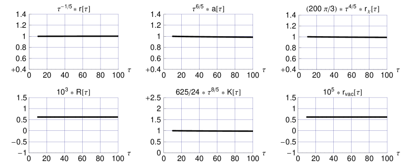
Figure 4: Numerical solution of the modified ODEs (40) with source term (42) and parameters $w_{M}=1/3$, $\zeta=1$, $\mu=3$, $\lambda=1$, and $\gamma=0$ (quantum-dissipative effects turned off). The initial boundary conditions are taken from the analytic solution (30), (31), and (36), for $\alpha=1$, but now with a type-3 perturbation (37c) for $\delta_{3}=+10^{-6}$. Specifically, the boundary conditions at $\tau=\tau_{\text{bcs}}=10$ are: $\{a,r,\dot{r},r_{\chi}\}$ $=$ $\{0.0630957450,1.58489478,0.03182679077,0.000756730758\}$, where the $\dot{r}$ value has been obtained from the first Friedman equation (41). The top row shows the three basic variables: the metric functions $r(\tau)$ and $a(\tau)$ and the dimensionless matter energy density $r_{\chi}$. The bottom row shows three derived quantities: the dimensionless Ricci curvature scalar $\mathcal{R}$, the dimensionless Kretschmann curvature scalar $\mathcal{K}$, and the dimensionless gravitating vacuum energy density $r_{\text{vac}}$ from (40d). The vacuum energy density from the initial conditions is $r_{\text{vac}}(\tau_{\text{bcs}})=6.16667\times 10^{-6}$, which stays essentially constant.

Observe, again, that the ODEs (40a) and (40c) with source term (42) are time-reversal noninvariant. The basic structure of the resulting vacuum-energy equation,

$$\dot{r}_{\text{vac}}=-\widetilde{\gamma}\;\big{|}\dot{r}/r\big{|}\;\big{(}r_{\text{vac}}\big{)}^{2}\,,$$ (43)

is similar to the one discussed in Refs. KlinkhamerVolovik-MPLA-2016 ; Klinkhamer2022-preprint , where, with a rapid switch-on, an analytic solution could be obtained for $r_{\text{vac}}(\tau)$ that drops to zero as $\tau\to\infty$.

The exact solution of Sec. VI.3 carries over to the modified ODEs (40) with source term (42) . The reason is simply that this source term $\Gamma$ vanishes if $r_{\text{vac}}=0$, which is precisely the case for our analytic solution.

VII.3 Numerical results

Numerical results from the original ODEs (28) for “mild” perturbations (keeping $r_{\text{vac}}\approx 0$) have been discussed in Sec VI.5. These results are essentially unchanged if we use the modified ODEs (40), as the source term (42) vanishes if $r_{\text{vac}}$ does. We then turn to the “dangerous” perturbations (making for nonzero $r_{\text{vac}}$ to leading order in the perturbation), for which we have introduced the modified ODEs (40) with the source term $\Gamma$ from (42).

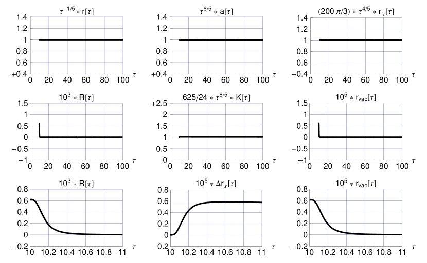
Figure 5: The boundary conditions at $\tau=\tau_{\text{bcs}}=10$ and the model parameters are the same as in Fig. 4, but now with $\gamma=2\times 10^{11}$ (quantum-dissipative effects turned on). The vacuum energy density is initially $r_{\text{vac}}(10)=6.16667\times 10^{-6}$ and drops to $r_{\text{vac}}(100)\sim 1\times 10^{-10}$. The bottom-middle panel shows the extra contribution to the matter energy density compared to that of the $\gamma=0$ numerical solution of Fig. 4, specifically $\Delta r_{\chi}(\tau)\equiv r_{\chi}(\tau)-r_{\chi}^{(\gamma=0,\,\text{num-sol})}(\tau)$.

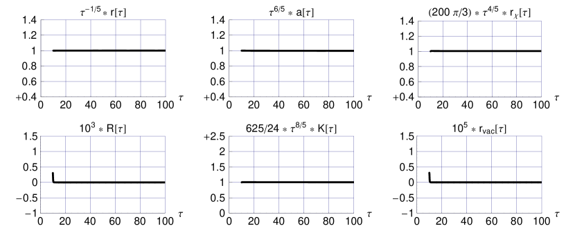
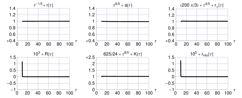
Figure 6: The model parameters and the boundary conditions at $\tau=\tau_{\text{bcs}}=10$ are the same as in Fig. 5, but now with a type-3 perturbation (37c) for $\delta_{3}=+5\times 10^{-7}$: $\{a,r,\dot{r},r_{\chi}\}$ $=$ $\{0.0630957397,1.584893985,0.03176239262,0.000756730758\}$, where the $\dot{r}$ value has been obtained from the first Friedman equation (41). The vacuum energy density is initially $r_{\text{vac}}(10)=3.08333\times 10^{-6}$ and drops to $r_{\text{vac}}(100)\sim 1\times 10^{-10}$.

Figure 7: The model parameters and the boundary conditions at $\tau=\tau_{\text{bcs}}=10$ are the same as in Fig. 5, but now with a type-3 perturbation (37c) for $\delta_{3}=+2\times 10^{-6}$: $\{0.0630957555,1.584896362,0.03195519835,0.000756730758\}$, where the $\dot{r}$ value has been obtained from the first Friedman equation (41). The vacuum energy density is initially $r_{\text{vac}}(10)=1.23334\times 10^{-5}$ and drops to $r_{\text{vac}}(100)\sim 2\times 10^{-10}$.

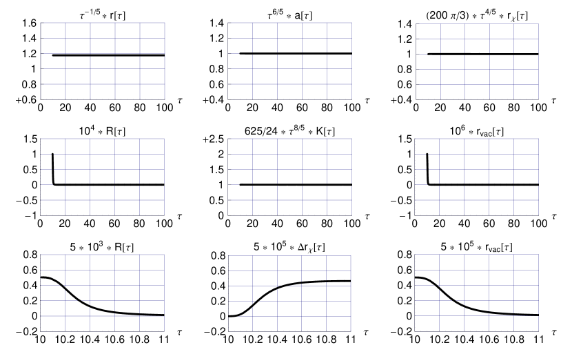
Figure 8: Numerical solution of the modified ODEs (40) with source term (42) and parameters $w_{M}=1/3$, $\zeta=1$, $\mu=3$, $\gamma=2\times 10^{11}$, and $\lambda=-1/4$ (different from the value $\lambda=1$ in Fig. 5). The initial boundary conditions are taken from the analytic solution (30), (31), and (36), for $\alpha=1$, but now with a type-3 perturbation (37c) for $\delta_{3}=+10^{-7}$. Specifically, the boundary conditions at $\tau=\tau_{\text{bcs}}=10$ are: $\{a,r,\dot{r},r_{\chi}\}$ $=$ $\{0.0630957355,1.86330736,0.0372908137,0.000756730758\}$, where the $\dot{r}$ value has been obtained from the first Friedman equation (41). The basic variables shown have been explained in the caption of Fig. 4 and $\Delta r_{\chi}$ from the bottom-middle panel is defined in the caption of Fig. 5. The vacuum energy density is initially $r_{\text{vac}}(10)=1.00208\times 10^{-6}$ and drops to $r_{\text{vac}}(100)\sim 2\times 10^{-10}$.

Numerical results, for $\mu=3$ and $\lambda=1$, are presented in Figs. 4 and 5 for boundary conditions from a type-3 perturbation (37c) with $\delta_{3}=+10^{-6}$ at $\tau=\tau_{\text{bcs}}=10$ and two values of the vacuum-matter energy-exchange coupling constant, $\gamma=0$ and $\gamma=2\times 10^{11}$. Focussing on the $r_{\text{vac}}$ panels in Fig. 5, we see that the modified ODEs (40) can cancel an initial positive vacuum energy density and get an asymptotic behavior close to that of the analytic Friedmann-type solution of Sec. VI.3 for $\alpha\approx 0.995$. A further remark on these $r_{\text{vac}}$ panels is that the drop of $r_{\text{vac}}(\tau)$ by about an order of magnitude occurs smoothly but rapidly, over the interval $\tau\in[10,\,10.3]$. A similar drop occurs for the Ricci curvature scalar (see the bottom-left panel of Fig. 5), which is consistent with the result $\mathcal{R}=32\,\pi\,r_{\text{vac}}\approx 100.53\,r_{\text{vac}}$ from the ODE (40b). Corresponding to the drop of the vacuum energy density (bottom-right panel of Fig. 5), there is an increase of the matter energy density (bottom-middle panel), but the match between both panels is not perfect, which may be due to the nonlinearity of the ODEs and the numerical accuracy.

For the same source term (42) with $\gamma=2\times 10^{11}$, different type-3 boundary conditions also give a relaxation to vanishing $r_{\text{vac}}$ (see Figs. 7 and 7). In short, we get, for $\mu=3$ and $\lambda=1$, a vanishing vacuum energy density $r_{\text{vac}}$ from a finite domain of initial conditions, namely $\delta_{3}\in[5\times 10^{-7},\,2\times 10^{-6}]$ for type-3 perturbations. Recall, that we also have finite domains for the type-1 and type-2 perturbations discussed in Sec. VI.5. There is, in fact, a finite 3-volume in the $\{a(\tau_{\text{bcs}}),\,r(\tau_{\text{bcs}}),\,r_{\chi}(\tau_{\text{bcs}})\}$ space (parametrized by $\delta_{1}\in[-0.1,\,+0.1]$, $\delta_{2}\in[-10^{-6},\,+10^{-6}]$, and $\delta_{3}\in[5\times 10^{-7},\,2\times 10^{-6}]$), whose corresponding solutions have $r_{\text{vac}}=\text{O}\left(10^{-5}\right)$ initially and $r_{\text{vac}}=\text{O}\left(10^{-10}\right)$ asymptotically.

Similar results have been obtained for other values of the cosmological constant, provided condition (32) holds. Numerical results for $\mu=3$ and $\lambda=-1/4$ are presented in Fig. 8. The numerical solution of Fig. 8 approaches asymptotically the analytic solution from Sec. VI.3 for $\widehat{r}_{\text{\,sol}}=(13/8)^{\,1/3}\approx 1.176$ and an $\alpha$ value approximately equal to $0.9992$.

The previous results start “close” to the analytic Friedmann-type solution in configuration space, but it is also possible to start “further away” in configuration space. Specifically, we can start from the analytic de-Sitter-type configuration as given in App. B. Numerical results, for $\mu=3$ and $\lambda=10^{-4}$, are presented in Figs. 9 and 10 with two values of the vacuum-matter-energy-exchange coupling constant $\gamma$. The numerical solution of Fig. 9 with $\gamma=0$ essentially reproduces the analytic solution of App. B, whereas the numerical solution of Fig. 10 with $\gamma=2\times 10^{11}$ shows the reduction of the vacuum energy density $r_{\text{vac}}$ and the approach to the analytic Friedmann-type solution of Sec. VI.3 [see, in particular, the bottom-row panels in Fig. 10 with $r(\tau)\propto\tau^{1/5}$, $a(\tau)\propto\tau^{-6/5}$, and $r_{\chi}(\tau)\propto\tau^{-4/5}$ ].

To summarize, it has been shown that the cosmological constant $\Lambda$ can, in principle, be cancelled by $\sqrt{-g}$ and appropriate quantum-dissipative effects. For completeness, we give, in App. C, further numerical results on how the vacuum energy density is cancelled before and after a phase transition, making concrete the general remarks in the last paragraph of Sec. IV.

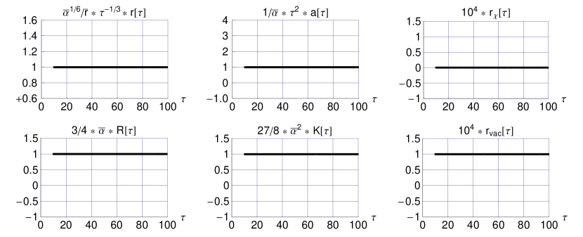
Figure 9: Numerical solution of the modified ODEs (40) with source term (42) and parameters $w_{M}=1/3$, $\zeta=1$, $\mu=3$, $\lambda=10^{-4}$, and $\gamma=0$ (quantum-dissipative effects turned off). The initial boundary conditions are taken from the analytic de-Sitter-type solution (51) and (54), having $\overline{\alpha}\equiv\alpha_{\text{deS-spec-sol}}=132.629$ and $\overline{r}\equiv r_{\text{deS-spec-sol}}=1.14471$. Specifically, the boundary conditions at $\tau=\tau_{\text{bcs}}=10$ are: $\{a,r,\dot{r},r_{\chi}\}$ $=$ $\{1.32629119,1.09208709,0.0364029029,0\}$, where the $\dot{r}$ value has been obtained from the first Friedman equation (41). The top row shows the three basic variables: the metric functions $r(\tau)$ and $a(\tau)$ and the dimensionless matter energy density $r_{\chi}$. The bottom row shows three derived quantities: the dimensionless Ricci curvature scalar $\mathcal{R}$, the dimensionless Kretschmann curvature scalar $\mathcal{K}$, and the dimensionless gravitating vacuum energy density $r_{\text{vac}}$ from (40d). The vacuum energy density from the initial conditions is $r_{\text{vac}}(\tau_{\text{bcs}})=1\times 10^{-4}$, which stays essentially constant.

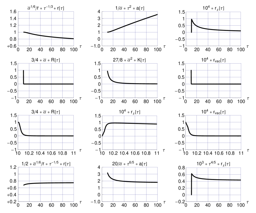
Figure 10: The boundary conditions at $\tau=\tau_{\text{bcs}}=10$ and the model parameters are the same as in Fig. 9, but now with $\gamma=2\times 10^{11}$ (quantum-dissipative effects turned on). The vacuum energy density is initially $r_{\text{vac}}(10)=1\times 10^{-4}$ and drops to $r_{\text{vac}}(100)\sim 2\times 10^{-10}$. The third row shows the behavior near the initial boundary conditions and the fourth row the asymptotic behavior.

VIII Final remarks

Perhaps the most interesting suggestion of this paper is the interpretation of the action (5) for $n(x)\propto\sqrt{-g(x)}$, as discussed in Sec. II. In the standard formulation of general relativity, this action is just a cosmological constant term with “$\mu$” proportional to the cosmological constant. Moreover, the action (5) is fully diffeomorphism invariant, but the integrand $n(x)\propto\sqrt{-g(x)}$ is not, as it is a scalar density.

If we now consider this $n(x)$ to be a physical quantity with $\mu$ in (5) interpreted as a chemical potential (possibly related to an underlying spacetime crystal), then $n(x)$ must be invariant under coordinate transformations and this implies that the only allowed coordinate transformations are those with unit Jacobian. In that case, it is possible that $n$ also enters the matter potential $\epsilon$, as discussed in Sec. IV. It is precisely this last step which makes for the “extension” mentioned in the title of the present paper. (The possibility of adding extra $\sqrt{-g}$ terms in the matter action was already noted on p. 220 of Ref. Zee1983 , but was not pursued further.)

The example potential $\epsilon$ from (14a) then shows that, for an appropriate range of $\mu$ values, the equilibrium value of $n$ can nullify the total gravitating vacuum energy density (14b). In a cosmological context as discussed in Secs. VI and VII, the dynamics of $n$ displays an attractor behavior towards Minkowski spacetime, provided quantum-dissipative effects are taken into account. The cosmological cancellation of an initial vacuum energy density, perhaps the most important result of this paper, is illustrated by Figs. 9 and 10.

There are two ingredients for this cosmic reduction of an initial vacuum energy density $\rho_{\text{vac}}$ (including a genuine cosmological constant $\Lambda$). First, the quantum-dissipative processes give an energy transfer from the vacuum component (with energy density $\rho_{\text{vac}}$ and equation-of-state parameter $w_{\text{vac}}=-1$) to a particle component (with $\rho_{M}$ and $w_{M}\geq 0$). Second, the expansion of the Universe does not affect the vacuum energy density [$\rho_{\text{vac}}(t)$ is constant] but does reduce the matter energy density [$\rho_{M}(t)$ drops with increasing cosmic scale factor $\widetilde{R}(t)$ from the Robertson–Walker metric (23)]. Such a two-step process has been considered before KlinkhamerVolovik-MPLA-2016 ; Klinkhamer2022-preprint . New, here, is that the vacuum variable is not a postulated quantity (such as a 4-form field strength or a 4D-brane density), but is provided by the already available spacetime metric, namely by its determinant.

Appendix A ANALYTIC FRIEDMANN-TYPE SOLUTION FOR GENERAL $\mathbf{w_{M}}$

We present in this appendix an exact solution of the ODEs (28) for matter equation-of-state parameter $w_{M}>-1$ and $\mu>0$ (similar results hold for $\mu<0$). As in the main text, we take the following Ansatz functions for $\tau>0$:

$$a(\tau) = \alpha\;\tau^{-2\,p}\,,$$ (44a)

$$r(\tau) = \alpha^{-1/6}\;\widehat{r}\;\tau^{p/3}\,,$$ (44b)

$$r_{\chi}(\tau) = \alpha^{-1}\;\widehat{\chi}\;\tau^{-m}\,,$$ (44c)

with positive parameters $\alpha$, $p$, $\widehat{r}$, $\widehat{\chi}$, and $m$. The vanishing of $r_{\text{vac}}$ from (28d) gives

$$\widehat{r}_{\text{\,sol}}=\left[\frac{\,1}{2\,\zeta}\;\big{(}\mu-\lambda\big{)}\right]^{1/3}\,,$$ (45)

where, for a given value $\mu>0$, the following condition holds on the dimensionless cosmological constant $\lambda$:

$$\lambda<\mu\,,$$ (46)

so that $\lambda$ can also be negative (see the last paragraph of this appendix for a related remark).

For the Ansatz functions (44), the dimensionless Ricci and Kretschmann curvature scalars read

$$\mathcal{R} = \frac{2}{3}\,p\,\big{(}5\,p-3\big{)}\,\frac{1}{\alpha}\,{\tau}^{-2\,(1-p)}\,,$$ (47a)

$$\mathcal{K} = \frac{4}{27}\,p^{2}\,\big{(}9-24\,p+17\,p^{2}\big{)}\,\frac{1}{\alpha^{2}}\,{\tau}^{-4\,(1-p)}\,.$$ (47b)

We look for an expanding ($p>0$) Friedmann-type universe approaching Minkowski spacetime (different from a de-Sitter spacetime at $p=1$).

With the Ansatz functions (44), the three ODEs from (28) reduce to the following expressions:

$$0 = \frac{1}{\alpha}\;\Big{(}p\,\left(1+w_{M}\right)-m\Big{)}\,\widehat{\chi}\,{\tau}^{-1-m}\,,$$ (48a)

$$0 = \frac{p^{2}}{3\,{\tau}^{2}}-8\,\pi\,\widehat{\chi}\,{\tau}^{-m-2\,p}\,,$$ (48b)

$$0 = \frac{p^{2}}{{\tau}^{2}}-\frac{2\,p}{3\,{\tau}^{2}}+8\,\pi\,w_{M}\,\widehat{\chi}\,{\tau}^{-m-2\,p}\,.$$ (48c)

The exact solution has arbitrary $\alpha>0$ and

$$p_{\text{\,sol}} = \frac{2}{3+w_{M}}\,,$$ (49a)

$$m_{\text{\,sol}} = \frac{2\,\left(1+w_{M}\right)}{3+w_{M}}\,,$$ (49b)

$$\widehat{\chi}_{\text{\,sol}} = \frac{1}{6\,\pi\,{\left(3+w_{M}\right)}^{2}}\,,$$ (49c)

where $p_{\text{\,sol}}$ ranges over $(0,\,1)$ for $w_{M}\in(-1,\,+\infty)$. Phrased differently, the analytic solution for fixed values of the model parameters $\mu$, $\lambda$, and $w_{M}$, has a one-dimensional modulus space $\mathbb{R}^{+}$ parametrized by $\alpha$.

The main points of the cosmology, with $w_{M}=1$ for example, are as follows:

• an expanding Friedmann-type universe with scale factor $r\sim\tau^{1/6}$.

• a perfect-fluid energy density and pressure $r_{\chi}(\tau)=p_{\chi}(\tau)\sim 1/\tau$.

• a cosmological constant cancelled by $\sqrt{-g}=\widehat{r}_{\text{\,sol}}$ from (45), provided condition (46) holds, so that $r_{\text{vac}}(\tau)=0$.

• the curvature scalars $\mathcal{R}(\tau)\sim 1/\tau$ and $\mathcal{K}(\tau)\sim 1/\tau^{2}$.

The overall behavior of this $w_{M}=1$ cosmology is not very different from that of Sec. VI.3, which had a $w_{M}=1/3$ perfect fluid.

Let us end with a parenthetical remark expanding on the third item of the previous paragraph. It is, namely, possible to relax condition (46) by changing the $\epsilon$ Ansatz (19b). An example, using dimensionless variables, is given by $\epsilon=\lambda+n+1/n^{2}$, which gives $r_{\text{vac}}=\lambda+2\,n-1/n^{2}-u$ from (12). In this $r_{\text{vac}}$ expression, any value of $\lambda-u$ can be cancelled by an appropriate real value $n=\overline{n}>0$.

Appendix B ANALYTIC DE-SITTER-TYPE SOLUTION

The ODEs (28) have an analytic Friedmann-type solution, as discussed in Sec. VI.3 and App. A. But there is also an analytic de-Sitter-type solution, which will be presented here.

As before, we assume the model parameters to obey the following conditions:

$$\zeta > 0\,,$$ (50a)

$$\mu > 0\,,$$ (50b)

$$\lambda < \mu\,,$$ (50c)

where the condition on the chemical potential $\mu$ is only to simplify the discussion (what really matters is that the combination $\mu-\lambda$ is positive). The Ansatz functions for $\tau>0$ are

$$a(\tau) = \alpha\;\tau^{-2\,p}\,,$$ (51a)

$$r(\tau) = \alpha^{-1/6}\;\widehat{r}\;\tau^{p/3}\,,$$ (51b)

$$r_{\chi}(\tau) = 0\,,$$ (51c)

with positive parameters $\alpha$, $p$, and $\widehat{r}$. The general de-Sitter-type solution (denoted “deS-gen-sol”) then has the following parameters:

$$p_{\text{deS-gen-sol}} = 1\,,$$ (52a)

$$\alpha_{\text{deS-gen-sol}} = 1/(24\,\pi\,r_{\text{vac-deS-gen-sol}})\,,$$ (52b)

$$r_{\text{vac-deS-gen-sol}} = \lambda+2\,\zeta\,(\widehat{r}_{\text{deS-gen-sol}})^{3}-\mu>0\,,$$ (52c)

$$\widehat{r}_{\text{deS-gen-sol}} > 0\,.$$ (52d)

The corresponding dimensionless Ricci and Kretschmann curvature scalars read

$$\mathcal{R}_{\text{deS-gen-sol}} = \frac{4}{3}\,\frac{1}{\alpha_{\text{deS-gen-sol}}}\,,$$ (53a)

$$\mathcal{K}_{\text{deS-gen-sol}} = \frac{8}{27}\,\frac{1}{\alpha_{\text{deS-gen-sol}}^{2}}\,.$$ (53b)

The above solution has $r_{\text{vac}}$ (or, equivalently, $\widehat{r}$ ) as a free parameter. For $\lambda>0$, a special solution (denoted “deS-spec-sol”) has vacuum energy density $r_{\text{vac}}=\lambda$ if the following parameters are chosen:

$$p_{\text{deS-spec-sol}} = 1\,,$$ (54a)

$$\alpha_{\text{deS-spec-sol}} = \frac{1}{24\,\pi\,\lambda}\,,$$ (54b)

$$\widehat{r}_{\text{deS-spec-sol}} = \sqrt[3]{\frac{\,\mu}{2\,\zeta}}\,.$$ (54c)

The dimensionless Ricci and Kretschmann curvature scalars are given by (53) with $\alpha_{\text{deS-gen-sol}}$ replaced by $\alpha_{\text{deS-spec-sol}}$.

Appendix C READJUSTMENT AFTER A PHASE TRANSITION

The readjustment of the vacuum variable $q$ to a cosmological phase transition has been discussed, in general terms, by Sec. II-C of Ref. KlinkhamerVolovik2008a . We expect a similar behavior of the metric-determinant vacuum variable $n$ from (3), especially as we have observed an attractor behavior in the numerical results of Secs. VI and VII. The present appendix aims to verify these expectations with a simplified setup. From now on, we will use only the dimensionless variables from Sec. VI.2.

Specifically, we model the phase transition by taking different $\lambda$ values before and after a cosmic time $\tau_{\text{PhT}}$ ,

$$\lambda(\tau)=\begin{cases}\lambda_{1}\,,&\text{for}\;\;\tau<\tau_{\text{PhT}}\,,\\[5.69054pt] \lambda_{2}\,,&\text{for}\;\;\tau>\tau_{\text{PhT}}\,.\end{cases}$$ (55)

Let us consider, for simplicity, the case $\lambda_{2}>\lambda_{1}>0$. Then, we will solve the modified ODEs (40) over the cosmic time interval $\tau\in[\tau_{\text{bcs}},\,\tau_{\text{PhT}})$ for $\tau_{\text{bcs}}<\tau_{\text{PhT}}$ and $\lambda=\lambda_{1}$ and over the interval $\tau\in(\tau_{\text{PhT}},\,\tau_{\text{max}}]$ for $\tau_{\text{PhT}}<\tau_{\text{max}}$ and $\lambda=\lambda_{2}$. At $\tau=\tau_{\text{PhT}}$, we take the metric functions $\{a(\tau),r(\tau),\dot{r}(\tau)\}$ to be continuous and the $r_{\chi}$ value just above $\tau_{\text{PhT}}$ from the first Friedman equation (41) with $\lambda=\lambda_{2}>\lambda_{1}$. (Different matching conditions are needed for the case $0<\lambda_{2}<\lambda_{1}$.)

Numerical results are shown in Fig. 11 for the case without vacuum-matter energy exchange ($\gamma=0$) and in Fig. 12 for the case with vacuum-matter energy exchange ($\gamma>0$). The results from Fig. 12 demonstrate that, as expected, the added vacuum energy from a phase transition can be rapidly cancelled by the metric-determinant vacuum variable, provided quantum-dissipative effects are included.

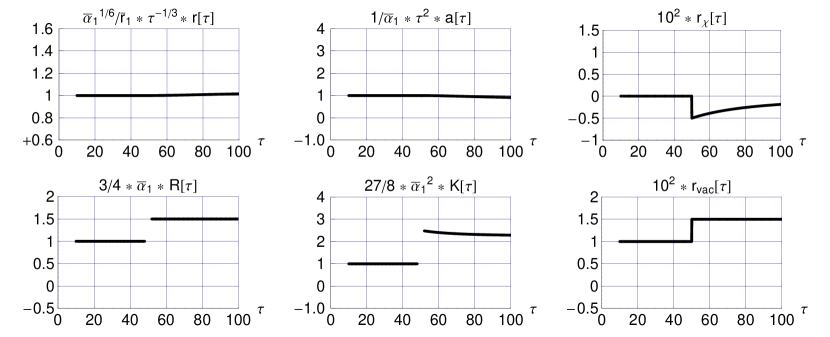
Figure 11: Numerical solution of the modified ODEs (40) with the source term (42) and the $\lambda$ stepfunction (55) modelling a cosmological phase transition at $\tau=\tau_{\text{PhT}}$, for parameters $w_{M}=1/3$, $\zeta=1$, $\mu=3$, $\lambda_{1}=10^{-2}$, $\lambda_{2}=1.5\times 10^{-2}$, and $\gamma=0$ (quantum-dissipative effects turned off). The initial boundary conditions at $\tau=\tau_{\text{bcs}}=10$ are taken from the analytic de-Sitter-type solution and are similar to those of Fig. 9. The boundary conditions at $\tau=\tau_{\text{PhT}}{}^{+}=50^{+}$ take the numerical function values of $\{a(\tau),r(\tau),\dot{r}(\tau)\}$ obtained just below $\tau_{\text{PhT}}$, while the $r_{\chi}(50^{+})$ value follows from the first Friedman equation (41) with $\lambda=\lambda_{2}$.

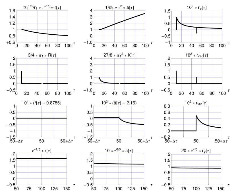
Figure 12: The boundary conditions at $\tau=\tau_{\text{bcs}}=10$ and the model parameters are the same as in Fig. 11, but now with $\gamma=2\times 10^{11}$ (quantum-dissipative effects turned on). The vacuum energy density starts from the value $r_{\text{vac}}(10)=1\times 10^{-2}$, drops to $r_{\text{vac}}(50^{-})\approx 2\times 10^{-10}$, then jumps to $r_{\text{vac}}(50^{+})\approx 0.5\times 10^{-2}$, and finally drops to $r_{\text{vac}}(100)\approx 3\times 10^{-10}$. The numerical results for $\mathcal{R}(\tau)$ and $\mathcal{K}(\tau)$ on the second row are not plotted at $\tau_{\text{PhT}}=50$, as the “spikes” there are primarily artifacts. The third row shows the behavior of the two metric functions and the vacuum energy density in a small interval around at $\tau_{\text{PhT}}=50$ with $\Delta\tau=10^{-6}$ [the left and middle panels use the combinations $\widehat{r}(\tau)\equiv\overline{\alpha}_{1}{\,}^{1/6}/\overline{r}_{1}\,\tau^{-1/3}\,r(\tau)$ and $\widehat{a}(\tau)\equiv 1/\overline{\alpha}_{1}\,\tau^{2}\,a(\tau)$, which are precisely the combinations from the top row]. The fourth row shows the asymptotic behavior of the two metric functions and the matter energy density.

References

- (1) S. Weinberg, “The cosmological constant problem,” Rev. Mod. Phys. 61, 1 (1989).
- (2) S.M. Carroll, “The cosmological constant,” Living Rev. Relativity 4, 1 (2001), arXiv:astro-ph/0004075.
- (3) F.R. Klinkhamer and G.E. Volovik, “Self-tuning vacuum variable and cosmological constant,” Phys. Rev. D 77, 085015 (2008), arXiv:0711.3170.
- (4) F.R. Klinkhamer and G.E. Volovik, “Dynamic vacuum variable and equilibrium approach in cosmology,” Phys. Rev. D 78, 063528 (2008), arXiv:0806.2805.
- (5) F.R. Klinkhamer and G.E. Volovik, Tetrads and -theory, JETP Lett. 109, 364 (2019), arXiv:1812.07046.
- (6) F.R. Klinkhamer and G.E. Volovik, “Big bang as a topological quantum phase transition,” Phys. Rev. D 105, 084066 (2022), arXiv:2111.07962.
- (7) J. Nissinen and G.E. Volovik, Elasticity tetrads, mixed axial-gravitational anomalies, and (3+1)-d quantum Hall effect, Phys. Rev. Res. 1, 023007 (2019), arXiv:1812.03175.
- (8) J. Nissinen, “Field theory of higher-order topological crystalline response, generalized global symmetries and elasticity tetrads,” arXiv:2009.14184.
-
(9)
A. Einstein,
“Spielen Gravitationsfelder im Aufbau
der materiellen Elementarteilchen eine wesentliche Rolle?”
(Do gravitational fields play an essential role
in the structure of the elementary particles of matter?),
Preussische Akademie der Wissenschaften Berlin,
Sizungsberichte (Math. Phys.), 1919, 349
(1919);
paper and translation available from
https://einsteinpapers.press.princeton.edu/vol7-doc/187andhttps://einsteinpapers.press.princeton.edu/vol7-trans/101. - (10) J.J. van der Bij, H. van Dam, and Y.J. Ng, “The exchange of massless spin two particles,” Physica (Amsterdam) 116 A, 307 (1982).
- (11) A. Zee, “Remarks on the cosmological constant problem,” in High-Energy Physics: Proceedings of Orbis Scientiae 1983, edited by S.L. Mintz and A. Perlmutter (Plenum Press, N.Y., 1985), pp. 211–230.
- (12) W. Buchmüller and N. Dragon, “Einstein gravity from restricted coordinate invariance,” Phys. Lett. B 207, 292 (1988).
- (13) M. Henneaux and C. Teitelboim, “The cosmological constant and general covariance,” Phys. Lett. B 222, 195 (1989).
- (14) D. Bensity, E.I. Guendelman, A. Kaganovich, E. Nissimov, and S. Pacheva, “Non-canonical volume-form formulation of modified gravity theories and cosmology,” Eur. Phys. J. Plus 136, 46 (2021), arXiv:2006.04063.
- (15) E. Alvarez and A.F. Faedo, “Unimodular cosmology and the weight of energy,” Phys. Rev. D 76, 064013 (2007), arXiv:hep-th/0702184.
- (16) V. Mukhanov, Physical Foundations of Cosmology (Cambridge University Press, Cambridge, England, 2005).
- (17) K. Bamba, S.D. Odintsov, and E.N. Saridakis, “Inflationary cosmology in unimodular gravity,” Mod. Phys. Lett. A 32, 1750114 (2017), arXiv:1605.02461.
- (18) F.R. Klinkhamer, “A generalization of unimodular gravity with vacuum-matter energy exchange,” Int. J. Mod. Phys. D 26, 1750006 (2016), arXiv:1604.03065.
- (19) F.R. Klinkhamer, M. Savelainen, and G.E. Volovik, “Relaxation of vacuum energy in -theory,” J. Exp. Theor. Phys. 125, 268 (2017), arXiv:1601.04676.
-
(20)
Ya.B. Zel’dovich and A.A. Starobinsky,
“Rate of particle production in gravitational fields,”
JETP Lett. 26, 252 (1977); paper available
from
http://jetpletters.ru/ps/1379/article_20902.pdf. - (21) F.R. Klinkhamer and G.E. Volovik, “Dynamic cancellation of a cosmological constant and approach to the Minkowski vacuum,” Mod. Phys. Lett. A 31, 1650160 (2016), arXiv:1601.00601.
- (22) F.R. Klinkhamer, “Q-field from a 4D-brane: Cosmological constant cancellation and Minkowski attractor,” to appear in LHEP, arXiv:2207.03453.