Filtering and imaging of frequency-degenerate spin waves using nanopositioning of a single-spin sensor

Abstract

Nitrogen-vacancy (NV) magnetometry is a new technique for imaging spin waves in magnetic materials. It detects spin waves by their microwave magnetic stray fields, which decay evanescently on the scale of the spin-wavelength. Here, we use nanoscale control of a single-NV sensor as a wavelength filter to characterize frequency-degenerate spin waves excited by a microstrip in a thin-film magnetic insulator. With the NV-probe in contact with the magnet, we observe an incoherent mixture of thermal and microwave-driven spin waves. By retracting the tip, we progressively suppress the small-wavelength modes until a single coherent mode emerges from the mixture. In-contact scans at low drive power surprisingly show occupation of the entire iso-frequency contour of the two-dimensional spin-wave dispersion despite our one-dimensional microstrip geometry. Our distance-tunable filter sheds light on the spin-wave band occupation under microwave excitation and opens opportunities for imaging magnon condensates and other coherent spin-wave modes.

Spin waves are collective spin excitations of magnetically ordered materials, with associated quasi-particles called magnons[1]. Due to their low damping, spin waves are promising as information carriers in information-technology devices[2, 3, 4, 5]. Techniques to image spin waves aid in studying such devices and realizing their technological potential. As such, several imaging techniques have been developed, with most established techniques based on the spin-dependent scattering of photons[6, 7, 8].

Nitrogen-vacancy (NV) magnetometry images spin waves by their microwave magnetic stray fields. It uses the electronic spin of the NV lattice defect in diamond as a sensor, which can be read out through spin-dependent photoluminescence (PL), is atomic-sized and can stably exist within nanometers from the diamond surface[9, 10]. This enables magnetic imaging with nanoscale spatial resolution and high sensitivity. The NV spin allows probing spin-wave spectra with a $\sim$1-MHz frequency resolution through spin lifetime measurements and characterizing spin-wave amplitudes by measuring the NV spin rotation rate[29]. Recently, NV magnetometry has been used to study domain-wall-guided spin-wave modes[12], magnon scattering[13, 30, 15], spin chemical potentials[16], and frequency combs[17]. To enable sensitivity to target spin-wavelengths, accurate control of the NV-sample distance is crucial because the spin-wave stray fields depend exponentially on the distance to the sample at a length scale set by their wavelength.

Here, we demonstrate that controlling the NV-sample distance using a diamond tip mounted on an atomic force microscope (Fig. 1a) creates a tunable wavelength filter that enables selective probing of frequency-degenerate spin-wave modes. Increasing the NV-sample distance progressively filters out small-wavelength spin waves, enabling studies of long-wavelength modes that are otherwise hidden in thermal spin-wave noise. We demonstrate high-contrast imaging over a range of wavelengths by adjusting the NV-sample distance on the nanoscale. When maximizing the wavenumber-cutoff of our distance-tunable filter via in-contact scans, we find a surprising pattern of standing spin waves instead of the expected traveling waves. Fourier transforms of the patterns reveal an occupation of spin-wave modes along the entire iso-frequency contour of the two-dimensional spin-wave dispersion despite our one-dimensional stripline geometry, which we attribute to spin-wave scattering. These results show that the exponential decay of the spin-wave stray fields provide a resource unique to magnetic-resonance spin-wave imaging, enabling wavenumber-selective detection of frequency-degenerate spin waves and high-resolution imaging of spin-wave scattering.

Our system consists of a thin film of yttrium iron garnet (YIG), a magnetic insulator with ultra-low spin-wave damping[18]. We excite spin waves by applying a microwave current to a stripline that is microfabricated onto the YIG surface (Fig. 1a, methods). We apply a bias field $B_{0}$ along the NV axis to tune the NV electron spin resonance (ESR) frequencies ($f_{\pm}$) relative to the spin-wave band. The orientation of $B_{0}$ magnetizes the film in-plane and perpendicularly to the stripline, enabling efficient excitation of ‘backward-volume’ spin waves[18] that travel parallel to the magnetization (Fig. 1b) (Supporting Information, Note S.1-S.2). The spin waves generate magnetic stray fields above the surface that drive our NV spin when resonant with an NV electron spin resonance (ESR) frequency. We detect these NV-resonant spin waves via the NV-center’s spin-dependent photoluminescence[19] (PL).

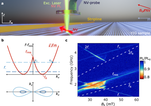
Figure 1: Imaging stripline-driven spin waves using scanning nitrogen-vacancy (NV) magnetometry. (a) A single NV spin embedded $\sim$20\text{\,}\mathrm{nm}$$ from the apex of a diamond tip measures the magnetic stray fields of spin waves excited by a microwave stripline in a $235\text{\,}\mathrm{nm}$-thick yttrium iron garnet (YIG) film. The NV spin is initialized using a green laser and read out via its spin-dependent photoluminescence (PL). A bias magnetic field $B_{0}$ is applied along the NV axis, magnetizing the film perpendicularly to the $1\text{\,}\mathrm{mm}$-long, $15\text{\,}\mathrm{\SIUnitSymbolMicro m}$-wide stripline. (b) Top: Calculated dispersion of spin waves traveling parallel to the YIG magnetization (‘backward-volume’ spin waves). The NV spin detects spin waves at its electron spin resonance (ESR) frequency, $f_{-}$, indicated by dashed lines for two values of $B_{0}$ (darker color corresponds to a larger $B_{0}$). In this work we focus on spin waves resonant with $f_{-}$ in the range $f_{\text{B}}<f_{-}<f_{\text{FMR}}$ for which there exist two frequency-degenerate backward-volume modes, $k_{1}$ and $k_{2}$. Bottom: iso-frequency contours of the two-dimensional spin-wave dispersion at the frequencies indicated by the dashed lines in the top panel. (c) NV photoluminescence as a function of $B_{0}$ and the microwave drive frequency. Data taken with the NV-tip in contact with the YIG at $\sim$30\text{\,}\mathrm{\SIUnitSymbolMicro m}$$ from the stripline edge at $1\text{\,}\mathrm{mW}$ drive power. The NV photoluminescence under microwave excitation (PL) is normalized to the NV photoluminescence without microwave excitation ($\text{PL}_{0}$). The ESR frequencies ($f_{\pm}$) and calculated FMR frequency $f_{\text{FMR}}$ are labelled. The dashed lines indicate the calculated minimum spin-wave frequency $f_{\text{B}}$ and its harmonic at $2f_{\text{B}}$.

We start by providing an overview of the NV PL as a function of the frequency of the microwave current applied to the stripline and the bias field $B_{0}$ (Fig. 1c). We do so with the diamond tip in contact with the YIG at $\sim$30\text{\,}\mathrm{\SIUnitSymbolMicro m}$$ from the stripline (methods). We observe several regions of reduced PL caused by NV spin transitions that provide a first insight into the spin waves excited by the stripline: First, two lines of reduced PL occur when the drive frequency is resonant with the NV ESR frequencies $f_{-}$ and $f_{+}$. Here, the NV spin is driven by the sum of the direct stripline field and the stray field of spin waves excited by the stripline[29, 30]. Second, a line of reduced PL reveals the YIG ferromagnetic resonance (FMR). Here, FMR-induced magnon-magnon scattering leads to spin-wave noise at the NV frequencies that causes NV spin relaxation and an associated PL reduction[13, 16]. Third, we observe a broad region of reduced PL when $f_{-}$ is in the vicinity of the FMR. In this region, the stripline efficiently excites spin waves because of their micron-scale wavelengths near the FMR (Supporting Information, Note S.2). These spin waves in turn scatter efficiently to modes resonant with $f_{-}$ because they are close in frequency and wavelength[20], causing NV spin relaxation. Correspondingly, the region of reduced PL ends abruptly when $f_{-}$ drops below the bottom of the spin-wave band (labelled $f_{\text{B}}$ in Fig. 1c) at $B_{0}\approx 41$ mT. In this work, we study spin waves in the region $f_{\text{B}}<f_{-}<f_{\text{FMR}}$ and use the nanoscale control of the NV tip as a wavelength filter to separate the contributions from frequency-degenerate incoherent and coherent spin waves.

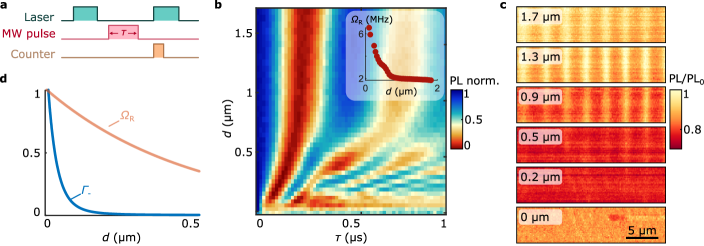
Figure 2: Tuning the NV-sample distance as a filter to selectively image a long-wavelength spin-wave mode. (a) Pulse sequence used for the measurement in (b): A $2.5\text{\,}\mathrm{\SIUnitSymbolMicro s}$ green laser pulse initializes the NV spin. A variable-duration microwave (MW)-pulse excites spin waves. The final NV spin state is read out by measuring the NV photoluminescence during the first $600\text{\,}\mathrm{ns}$ of a second green laser pulse. (b) Spin-wave-driven NV spin dynamics vs tip-sample distance $d$. The dynamics are governed by the stray-field spectrum of the spin waves at the NV frequency. For $d\gtrsim$100\text{\,}\mathrm{nm}$$, the stray field of a coherent spin wave yields high-visibility Rabi oscillations with a long decay time. Below $\sim$100\text{\,}\mathrm{nm}$$, the Rabi decay time starts to vanish, attributed to the more rapidly increasing stray field generated by thermal spin waves (see (d)). Measurement taken at $31\text{\,}\mathrm{\SIUnitSymbolMicro m}$ from the stripline edge at $B_{0}=$32\text{\,}\mathrm{mT}$$, $f_{-}=$1.98\text{\,}\mathrm{GHz}$$ and $P_{\text{MW}}=$6.3\text{\,}\mathrm{mW}$$. Inset: Fitted Rabi frequency vs $d$ down to $100\text{\,}\mathrm{nm}$. (c) Spatial maps of the ESR contrast while driving spin waves at $f_{-}=$1.89\text{\,}\mathrm{GHz}$$ and $B_{0}=$35\text{\,}\mathrm{mT}$$ at $P_{\text{MW}}=$1\text{\,}\mathrm{mW}$$ for varying $d$. The ESR contrast is obtained by normalizing the NV photoluminescence under microwave excitation (PL) to that without microwave excitation ($\text{PL}_{0}$). (d) Calculation comparing the NV relaxation rate $\Gamma_{-}$ caused by thermal spin waves to the NV Rabi oscillation rate caused by a coherently driven spin wave. Both rates are normalized to their value at $d=0$ to highlight the different scaling with distance. The calculation of $\Gamma_{-}$ assumes an equal population of all spin-wave modes at frequency $f_{-}$ as expected for a Rayleigh-Jeans distribution[28]. The calculation of $\Omega_{\text{R}}$ assumes only a single spin-wave mode with wavenumber $k=$2\text{\,}{\mathrm{\SIUnitSymbolMicro m}}^{-1}$$ (as imaged in (c)) is excited.

Spin waves generate a rotating magnetic stray field with amplitude $B_{\text{SW}}$ that decays with increasing distance $d$ to the sample[28], with the decay length set by the spin-wavenumber $k$ according to:

$$B_{\text{SW}}\propto ke^{-kd}$$ (1)

As such, increasing the NV-sample distance progressively filters out the stray fields of high-wavenumber spin waves (Supporting Information, Note S.3). We demonstrate the filtering by characterizing the stray fields of spin waves excited by the microwave stripline as a function of the NV-sample distance. We do so by measuring the NV spin rotation rate (Rabi frequency), which depends linearly on the amplitude of the NV-resonant microwave field. We measure the Rabi frequency by tuning the NV frequency $f_{-}$ to the iso-frequency contour of figure 1b and applying variable-duration microwave pulses. These pulses excite $f_{-}$-resonant spin waves that drive NV spin rotations via their magnetic stray field[22] (Fig. 2a-b).

With the tip in contact with the YIG (Fig. 2b, $d=0$ nm), we observe fast NV spin decoherence, indicating a strong presence of incoherent spin-wave noise. As further shown below, the noise is caused by a combination of thermal and microwave-excited spin wave modes. By lifting the NV a few hundreds of nanometers, we suppress the noise sufficiently and start observing NV Rabi oscillations, indicating a coherent microwave field at the NV frequency. The non-exponential decrease of the Rabi frequency with a further increasing $d$ (Fig. 2b and its inset) shows that the Rabi oscillations are driven by an ensemble of coherent spin waves of which the high wavenumbers are progressively suppressed by the distance-dependent cutoff of the filter.

Using spatial maps of the ESR contrast (Fig. 2c), we demonstrate that the distance-tunable filter enables spatial imaging of a single low-$k$ spin wave within an ensemble of frequency-degenerate spin-wave modes. We define the contrast $C$ by the ratio of the NV PL with and without microwave drive ($C=1-\text{PL}/\text{PL}_{0}$). The spatial contrast arises due to the interference between the field of the excited spin waves (which are propagating) and the uniform reference field that is supplied by our stripline[29, 30]. The in-contact scan (bottom panel Fig. 2c) shows two important features: first, the maximum contrast, $C_{\text{max}}(d=0)=0.15$, is reduced with respect to the maximum contrast at increased distances $C_{\text{max}}(d>$200\text{\,}\mathrm{nm}$)=0.25$. Second, the contrast equals its maximum value throughout the scan (i.e., it is saturated). We attribute the reduced contrast of the in-contact scan to the strong distance dependence of the stray fields generated by thermally excited spin waves (Fig. 2d), which cause NV relaxation and PL reduction in the absence of the microwave drive[28, 23](Supporting Information, Note S.4). The spatially homogeneous saturation indicates a large amplitude of the microwave-driven spin waves, as we will show in more detail below.

Retracting the tip to $d=$0.2\text{\,}\mathrm{\SIUnitSymbolMicro m}$$, we find that the contrast approximately doubles with respect to $d=$0\text{\,}\mathrm{\SIUnitSymbolMicro m}$$. This is expected from the rapid suppression of the thermal spin-wave stray fields by our filter. However, we still find that the contrast is saturated over the entire spatial map (Fig. 2c) due to the large stray fields of spin waves excited by the microwave drive. For distances $d>$1\text{\,}\mathrm{\SIUnitSymbolMicro m}$$, the microwave-driven spin waves are filtered to an extent that yields a clear spatial image of a single low-$k$ spin-wave mode (Fig. 2c). These results show how lifting the tip from the surface filters out high-$k$ spin waves, enabling high-contrast imaging of a single low-$k$ spin wave within an ensemble of thermal and coherent spin-wave modes.

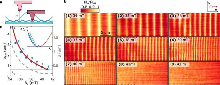
Figure 3: Adapting the sensor-to-sample distance to realize high-contrast imaging of different spin-wavelengths. (a) Spin waves generate a magnetic stray field that decays exponentially at the scale of the spin-wavelength. We tune the tip-sample distance $d$ to optimize the detection of different wavelengths. (b) Spatial maps of the NV ESR contrast showing backward-volume spin waves excited by the stripline at different magnetic fields $B_{0}$. Increasing $B_{0}$ (panels 1-8) decreases the wavelength of the spin waves that are resonant with the NV ESR frequency. In each scan, we tune the distance $d$ to maintain a constant ESR contrast, as plotted in c. In panel 8, we extract the wavelength by analyzing the dashed box. Drive power $P_{\text{MW}}=$4\text{\,}\mathrm{mW}$$. (c) The wavelengths extracted by fitting (Supporting Information Note S.5) the wave patterns in b (blue dots) compared to the wavelengths calculated from the backward-volume dispersion (plotted in red, Supporting Information, Note S.1), as a function of $B_{0}$. The wavelength at the minimum of the spin-wave band is indicated by $\lambda_{\text{B}}$. Grey dashed line (right y-axis): The tip-sample distance $d$ used in each of the scans shown in b. Inset, red line: calculated dispersion of the backward-volume spin waves relative to the minimum spin-wave frequency. Blue dots: modes imaged in b.

Fast NV-imaging of spin waves requires a strong ESR contrast. Because the spin-wave stray field falls off exponentially (Eq. 1), maintaining a strong contrast requires adapting the NV-sample distance to the expected spin-wavelength (Fig. 3a). We change the wavelength of the mode, indicated by $k_{1}$ in figure 1b, by increasing $B_{0}$ while reducing the drive frequency according to $f_{-}=D-\gamma B_{0}$ to maintain resonance with the NV, where $D=$2.87\text{\,}\mathrm{GHz}$$ is the NV zero-field splitting and $\gamma=$28\text{\,}\mathrm{GHz}\text{\,}{\mathrm{T}}^{-1}$$ is the electron gyromagnetic ratio. Starting from the distance used in figure 2c for $B_{0}=$35\text{\,}\mathrm{mT}$$, we find that keeping $kd=constant$ yields high-contrast images over a range of wavelengths (Fig. 3b). The spatial images of figure 3b show how the wavelength decreases with increasing $B_{0}$ until the $f_{-}$ detection frequency drops below the bottom of the spin-wave band at $B_{0}\approx$41\text{\,}\mathrm{mT}$$ (inset Fig. 3c). The large ESR contrast enables a straightforward extraction of the wavelengths (Supporting Information Note S.5), which correspond well with the calculated spin-wave dispersion (Fig. 3c).

Bringing the NV-tip into contact with the sample maximizes the wavenumber cutoff of our filter and increases the relative contribution of high-wavenumber modes to the stray field (Supporting Information, Note S.3). We use in-contact scans to study the ensemble of spin-wave modes excited in the magnetic film. To avoid the in-contact saturation observed in figure 2c, we tune down the drive power by a factor 500, which reveals a rich pattern of spin waves in different directions (Fig. 4a).

To interpret the wavenumber content of the spin-wave patterns observed in figure 4a, we perform a Fourier transform. The Fourier maps reveal the excitation of spin-wave modes along the entire $f_{-}$-isofrequency contour of the two-dimensional spin-wave dispersion (Fig. 4b). Although these modes are not directly excited by our microstrip, such an homogeneous occupation of the spin-wave dispersion may be expected when taking into account scattering of the primarily excited backward-volume spin waves[24] enhanced by the presence of defects in our film[32, 33] (Supporting Information, Note S.6).

Surprisingly, the absence of ESR contrast for fields larger than $40\text{\,}\mathrm{mT}$ (Supporting Information, Note S.7) shows that the amplitude of the direct stripline field is insufficient to generate the observed standing-wave pattern in the magnetic stray field. We therefore conclude that the observed spin waves are standing waves, created by scattered waves that have a fixed phase relation with the stripline drive field. These results highlight the coherent nature of the scattering process and the efficiency by which it leads to the occupation of high-momentum modes that are otherwise inaccessible to a one-dimensional excitation stripline.

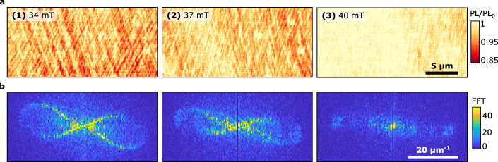
Figure 4: Emergence of frequency-degenerate, standing spin-wave modes in spatial maps of the ESR contrast. (a) Measured ESR contrast when the tip is in contact with the sample at low drive power ($6.3\text{\,}\mathrm{\SIUnitSymbolMicro W}$) for different magnetic bias fields $B_{0}$. (b) Absolute value of the Fourier-transformations of the maps in (a), revealing the wavevectors present in the spatial spin-wave patterns. The full isofrequency contour of the spin-wave dispersion is visible at $B_{0}=$34\text{\,}\mathrm{mT}$$.

Nanoscale control of the NV-sample distance serves as a tunable filter that enables balancing the magnetic fields generated by an ensemble of incoherent and coherently driven spin waves of different wavelengths. This control enables selective imaging of a coherent spin-wave mode within a mixture of frequency-degenerate spin waves and retaining a high-visibility response when imaging different wavelengths. In-contact scans at reduced drive power show a surprising pattern of standing spin-wave modes. The Fourier transforms of these patterns reveal spin-wave occupation along the entire iso-frequency contour of the two-dimensional spin-wave dispersion. We attribute the occupation of these high-momentum modes to defect-enhanced spin-wave scattering. The phase relation between the scattered modes is maintained, emphasizing the coherent nature of the scattering process. Nanoscale control of the NV-sample distance and wavenumber-selective imaging of magnetic oscillations at microwave frequencies paves the way for imaging magnon condensates[27] or other coherent spin-wave modes[12], and could also be used to probe microwave electric current distributions in devices.

Methods

YIG Sample

The $\sim$235(10)\text{\,}\mathrm{nm}$$ thick yttrium iron garnet (YIG) was grown on a gadolinium gallium garnet (GGG) substrate by liquid-phase epitaxy (Matesy GmbH). The YIG chip was first sonicated in acetone to remove contaminants. A $1\text{\,}\mathrm{mm}$-long and $15\text{\,}\mathrm{\SIUnitSymbolMicro m}$-wide stripline ($5\text{\,}\mathrm{nm}$ titanium / $200\text{\,}\mathrm{nm}$ gold) for spin-wave excitation was then deposited on top of the YIG surface using e-beam evaporation preceded by e-beam lithography, using a double PMMA resist (A8 495K / A3 950K) and a top layer of Elektra95.

Measurement Setup

Our scanning NV-magnetometry setup consists of two stacks of Attocube positioners (ANPx51/RES/LT) and scanners (ANSxy50/LT and ANSz50/LT) that enable individual positioning of the tip and sample, in addition to a confocal microscope setup, which are all placed in an acoustical enclosure. The confocal setup uses a $515\text{\,}\mathrm{nm}$ green laser (Cobolt 06-MLD, pigtailed) for NV excitation, which is focused by the objective lens (LT-APO/VISIR/0.82) onto a single-NV tip with the NV located approximately $20\text{\,}\mathrm{nm}$ below the tip surface ((001)-oriented, Qzabre). The NV photoluminescence (PL) is collected by the same objective and separated from the excitation laser by a dichroic mirror (Semrock Di03-R532-t3-25x36) and a long-pass filter (Semrock BLP01-594R-25), spatially filtered by a pinhole ($50\text{\,}\mathrm{\SIUnitSymbolMicro m}$), and finally collected by an avalanche photodiode (APD) (Excelitas SPCM-AQRH-13). A SynthHD (v2) microwave generator (Windfreak Technologies, LLC) was used to apply microwave signals. A programmable pulse generator (SpinCore Technologies, Inc. PulseBlasterESR-PRO 500) controls the timing of the laser excitation, detection window and microwaves. A National Instruments card (PCIe 6323) was used for the data acquisition.

Spin-wave imaging

All measurements were performed close to the middle of the $1\text{\,}\mathrm{mm}$-long stripline to prevent edge effects from stripline corners, within $30\text{\,}\mathrm{\SIUnitSymbolMicro m}$ from the edge of the $15\text{\,}\mathrm{\SIUnitSymbolMicro m}$-wide stripline. The direct stripline field interferes with the spin-wave field to form the standing-wave stray-field patterns of figures 2 and 3 [29, 30]. The static field $B_{0}$ is applied by moving a small permanent magnet mounted on translation stages. For all measurements, the magnet is aligned along the NV axis within $\sim$5\text{\,}\mathrm{\SIUnitSymbolDegree}$$ such that the expected angle between the NV and the sample is $\theta\approx$54\text{\,}\mathrm{\SIUnitSymbolDegree}$$ with respect to the sample-plane normal. Because of some uncertainty introduced when mounting the NV-probe, we leave this angle as a free parameter when fitting the measured wavelength to the spin-wave dispersion, yielding $\theta=$49\text{\,}\mathrm{\SIUnitSymbolDegree}$$ (Fig. 3d). For the scans at non-zero tip-sample distances in figures 2 and 3, we first touch down onto the sample with the tip to acquire a well-defined distance reference. Then, we turn off the AFM feedback and set the lift height using our piezo scanner (Supporting Information, Note S.8). We repeat this for each line trace. As there is no feedback, the lift height can change over a line trace due to drift or sample tilt.

Supporting Information

S.1 Spin-wave dispersion

Here, we calculate the spin-wave dispersion of our 235 nm film of yttrium iron garnet (YIG). We assume a 2D geometry, where the magnetization does not change across the film thickness (Fig. S.1). We first consider the relevant energy contributions for our magnetic system to evaluate the Landau-Liftshitz-Gilbert (LLG) equation that describes the dynamics of the magnetization. Following the approach described by Rustagi et. al[28], we then obtain the magnetic susceptibility (section S.1.1) and the spin-wave dispersion (section S.1.3).

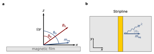
Figure S.1: Schematic of the measurement geometry. (a) Side view of our measurement geometry. The magnetic field is applied at an angle $\theta_{B}$ with respect to the sample normal. As a result the equilbrium magnetization $\vec{m}_{\mathrm{eq}}$ tilts slightly out-of-plane with an angle $\theta_{0}$. (b) Top view of the measurement geometry. We drive the transverse magnetization via an oscillating magnetic field supplied by a microwave current that is sent through a microstrip with width $15\text{\,}\mathrm{\SIUnitSymbolMicro m}$ and length $1\text{\,}\mathrm{mm}$. In this work, the stripline field excites spin waves that travel parallel to the equilibrium magnetization, also called backward-volume spin waves.The parameters used for calculating the spin-wave dispersion for the film studied in this work are: $M_{s}=1.42\cdot 10^{5}$ A/m, $A_{\mathrm{ex}}=3.8\cdot 10^{-12}$ J/m, $\alpha=1\cdot 10^{-4}$ and $L=235$ nm [29]. The angle between the magnetic field and the film, $\theta_{B}$ is $\theta_{B}\approx\theta_{\mathrm{NV}}\approx 54$°.

S.1.1 Magnetic susceptibility

Given that the Zeeman interaction, the demagnetizing field and the exchange interaction are the relevant energy contributions, we calculate the response of the transverse magnetization $\delta\vec{m^{\prime}}_{\perp}$ to a drive field $\vec{h}_{\perp}(\vec{k})$ via $\delta\vec{m^{\prime}}_{\perp}=S\vec{h}_{\perp}$. Here, $\delta\vec{m}^{\prime}$ is defined in the magnet frame, where the equilibrium magnetization ($\vec{m}_{\mathrm{eq}}$) points in the $z$-direction. And $S$ is the transverse magnetic susceptibility, which is given by [28]:

$$S(\vec{k},\omega)=\frac{\gamma}{\Lambda}\begin{bmatrix}\omega_{3}-i\alpha\omega&-\omega_{1}-i\omega\\ -\omega_{1}+i\omega&\omega_{2}-i\alpha\omega\end{bmatrix}$$ (S.1)

where

$$\omega_{0}(\vec{k}) =\omega_{\text{B}}\cos(\theta_{B}-\theta_{0})-\omega_{\text{M}}\cos^{2}\theta_{0}+\omega_{D}k^{2},$$ (S.2)

$$\omega_{1}(\vec{k}) =\omega_{\text{M}}f_{L}\sin\phi_{k}\cos\phi_{k}\cos\theta_{0},$$ (S.3)

$$\omega_{2}(\vec{k}) =\omega_{0}+\omega_{\text{M}}\left[f_{L}\cos^{2}\phi_{k}\cos^{2}\theta_{0}+(1-f_{L})\sin^{2}\theta_{0}\right],$$ (S.4)

$$\omega_{3}(\vec{k}) =\omega_{0}+\omega_{\text{M}}f_{L}\sin^{2}\phi_{k},$$ (S.5)

$$\Lambda(\omega) =(\omega_{2}-i\alpha\omega)(\omega_{3}-i\alpha\omega)-\omega_{1}^{2}-\omega^{2}.$$ (S.6)

Here, $\omega_{B}=\gamma B_{0}$, is the frequency associated with the Zeeman energy, where $\gamma$ is the gyromagnetic ratio and $B_{0}$ the externally applied magnetic field. We apply $B_{0}$ at an angle $\theta_{B}$, which is the direction of the magnetic field with respect to the sample normal, such that it aligns with the NV center. As a result, the equilibrium magnetization $\theta_{0}$ tilts out-of-plane by an angle $\theta_{0}$. Next, the frequency associated with the demagnetizing field is given by: $\omega_{M}=\gamma\mu_{0}M_{s}$, where $\mu_{0}$ and $M_{s}$ are the vacuum permeability and the saturation magnetization respectively. Finally, $\omega_{D}=\frac{\gamma D}{M_{s}}$ is associated with the exchange interaction, where $D$ is the spin stiffness. A wave vector, $\vec{k}$ is described by its wavenumber $k$ (i.e. the modulus of the wave vector) and by its direction which is described by $\phi_{k}$. Finally, the prefactor $f_{L}$ is given by $f_{L}\equiv 1-(1-e^{-kL})/(kL)$ in which $L$ is the film thickness.

S.1.2 Equilibrium magnetization

The equilibrium angle of the magnetization, $\theta_{0}$, follows from minimizing the free energy and solving for each value of the magnetic field:

$$-2B_{0}\sin(\theta_{B}-\theta_{0})=\mu_{0}M_{s}\sin(2\theta_{0})$$ (S.7)

We calculate that $\theta_{0}$ is in-plane to within a few degrees for the magnetic fields used in our measurements.

S.1.3 Spin-wave dispersion

The spin-wave dispersion is given by the frequencies for which the susceptibility is singular, i.e. when: $\Lambda=0$ (Fig. S.2).By tuning the external magnetic field, we vary $f_{-}$ with respect to the minimum spin-wave frequency, as such the contour (dashed line in Fig. S.2) changes shape such that $f_{-}$ becomes resonant with spin waves of different wavevectors.

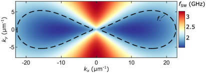
Figure S.2: Spin-wave dispersion. Calculated spin-wave dispersion for $B_{0}=$35\text{\,}\mathrm{mT}$$, i.e. when $f_{\mathrm{B}}<f_{-}<f_{\mathrm{FMR}}$. The field is aligned along the NV-axis such that $f_{-}=1.89$ $\mathrm{GHz}$, which is represented by the iso-frequency contour (dashed line).

S.2 Stripline field

We use a stripline oriented along $y$, with width $w$, length $L$ and thickness $h$ for spin-wave excitation, centered at $x=0$ and $z=-h/2$. A microwave current density $J(\omega)$ applied to the stripline generates a magnetic field with components [29]:

$$h_{\mathrm{x}}=2J(\omega)e^{kz}\frac{e^{kh}-1}{kk_{x}}\sin(k_{x}\frac{w}{2})\frac{\sin(k_{y}\frac{L}{2})}{k_{y(x)}}$$ (S.8)

$$h_{\mathrm{z}}=-2iJ(\omega)e^{kz}\frac{e^{kh}-1}{k^{2}}\sin(k_{x}\frac{w}{2})\frac{\sin(k_{y}\frac{L}{2})}{k_{y}}$$ (S.9)

in k-space. Because the film is magnetized along $x$, the x-component of the field does not contribute to spin-wave excitation. As such, we only consider the $z-$component. The field exciting the spin waves is obtained by averaging over the film thickness:

$$\tilde{h}_{z} =-2iJ(\omega)\frac{e^{-kL}-1}{kL}\frac{e^{kh}-1}{k^{2}}\sin(k_{x}\frac{w}{2})\frac{\sin(k_{y}\frac{L}{2})}{k_{y}}$$ (S.11)

Because the length of the stripline far exceeds its width and the distance between the stripline center and our measurement location, it is essentially a one-dimensional stripline that does not excite spin waves in the $k_{y}$ direction. (Fig. S.3).

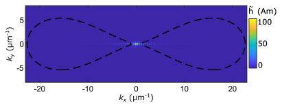
Figure S.3: The effective field strength for a stripline that is aligned perpendicular to the magnetization (backward-volume geometry). Using a $15\text{\,}\mathrm{\SIUnitSymbolMicro m}$-wide and $1\text{\,}\mathrm{mm}$-long stripline. The stripline field is most efficient in driving low-wavenumber modes (close to the FMR). Due to its one-dimensional character, spin waves with a component in the $k_{y}$ direction are not excited. Dashed line indicates the $f_{-}$-isofrequency contour (Fig. S.2) of NV resonant modes at 35 mT.

S.3 Wavenumber-dependent filtering of the spin-wave stray field

The measured spin-wave stray field is proportional to a prefactor $f_{k}$ that is dependent on the NV-to-sample distance ($d$) according to:

$$B_{\mathrm{SW}}\propto f_{k}=k\exp(-kd)$$ (S.12)

Here, $f_{k}$ is the ’filter function’ responsible for the wavenumber-filtering action of the measured spin-wave stray fields. The filter peaks at $k=1/d$ (Fig. S.4). We see that increasing the NV-sample distance progressively filters out the stray fields of the short wavelength spin-wave modes.

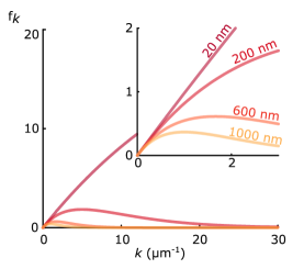
Figure S.4: Wavenumber selective filtering by tuning the NV-to-sample distance $d$. The filter function $f_{k}$ peaks at $k=1/d$, where $k$ is the spin-wavenumber. The filter function is plotted for several values of the NV-to-sample distance

S.4 NV relaxation induced by thermal magnons

We follow the approach of Rustagi et al.[28] to calculate the NV relaxation rates induced by the magnons in our YIG film (Fig. 2d, main text) using:

$$\Gamma_{\mp}(\omega_{\mp})=\frac{\gamma^{2}}{2}\int\frac{d\vec{k}}{(2\pi)^{2}}\sum_{{i,j}\in\{x,y\}}\mathcal{D}^{\text{eff}}_{\pm i}(\vec{k})\mathcal{D}^{\text{eff}}_{\mp j}(-\vec{k})C_{ij}(\vec{k},\omega_{\mp}).$$ (S.13)

Here, $\Gamma_{\mp}$ are the relaxation rates corresponding to the $\omega_{\mp}$ ESR frequencies, $\vec{k}$ is the spin-wavevector, $\mathcal{C}$ is a spin-spin correlator describing the thermal magnon fluctuations, and $\mathcal{D}^{\text{eff}}$ is a dipolar tensor that calculates the magnetic stray fields that induce NV spin relaxation generated by these fluctuations. Note, this equation is defined in the magnet frame, for which the equilibrium magnetization is along the $z$-direction.

The thermal transverse spin fluctuations in the film are described by [28]:

$$C_{ij}(\vec{k},\omega)=2D_{th}\sum_{\nu=\{x,y\}}S_{i\nu}(\vec{k},\omega)S_{j\nu}(-\vec{k},-\omega)$$ (S.14)

where $D_{\text{th}}=\frac{\alpha k_{B}T}{\gamma M_{\text{s}}L}$, with $k_{B}$ the Boltzmann constant, $T$ the temperature, $S$ the magnetic susceptibility (Eq. S.1).

The dipolar tensor $D^{\text{eff}}(\vec{k},\omega)$ is obtained by first rotating the magnet frame to the lab frame, then multiplying by the dipolar tensor $\mathcal{D}(\vec{k})$ in the lab frame, and then rotating the result to the NV frame: $D^{\text{eff}}(\vec{k},\omega)=R_{yz}(\theta_{\text{NV}},\phi_{\text{NV}})\mathcal{D}(\vec{k})R_{Y}(\theta_{0})^{T}$, where

$$\mathcal{D}(\vec{k})=-\frac{\mu_{0}M_{s}}{2}e^{-|\vec{k}|d_{\text{NV}}}(1-e^{-|\vec{k}|L})\begin{bmatrix}\cos^{2}\phi_{k}&\sin(2\phi_{k})/2&i\cos\phi_{k}\\ \sin(2\phi_{k})/2&\sin^{2}\phi_{k}&i\sin\phi_{k}\\ i\cos\phi_{k}&i\sin\phi_{k}&-1\end{bmatrix},$$ (S.15)

where $\mu_{0}$ is the vacuum permeability and $d_{\text{NV}}$ is the distance between the NV and the sample surface. The terms in Eq. (S.13) that induce spin relaxation are given by[28]: $\mathcal{D}^{\text{eff}}_{\pm\nu}=\mathcal{D}^{\text{eff}}_{x\nu}\pm i\mathcal{D}^{\text{eff}}_{y\nu}$.

For a magnon gas in thermal equilibrium, in the absence of microwave driving, the dependence of the NV relaxation rate on the NV-sample distance can be calculated using Eq. (S.13). The fast increase in rate (Fig. 2d, main text) results in a reduction of the ESR contrast as the NV sensor approaches the film to within nanometer proximity.

S.5 Spatial ESR contrast generated by a single spin wave

Here, we determine the spatial profile of the ESR contrast generated by a propagating spin-wave mode, with wavenumber $k$ that interferes with an uniform reference field of varying amplitude (Fig. S.5)[30, 29]. We show that the ESR contrast spatially varies depending on the wavenumber given that the reference field has a finite amplitude.

Spin waves produce a field of which the component ($B_{\text{SW}}$) that is rotating with the correct handedness in a plane that is perpendicular to the NV-axis drives Rabi oscillations[29]. This component varies spatially according to:

$$B_{\text{SW}}=B^{0}_{\text{SW}}e^{ik(x-x_{0})}$$ (S.16)

This field induces NV Rabi oscillations of which the rate is given by:

$$\Omega_{R}=\frac{\gamma}{\sqrt{2}}|B_{\text{SW}}+B_{\text{ref}}|$$ (S.17)

where $B_{\text{ref}}$ is the component of the reference field that is rotating with the correct handedness in a plane perpendicular to the NV-axis. The ESR contrast is given by:

$$\mathrm{PL}/\mathrm{PL}_{0} =1-C_{\text{ESR}}$$ (S.18)

$$\mathrm{PL}/\mathrm{PL}_{0} =1-\beta\frac{\Omega^{2}_{R}}{\Omega^{2}_{R}+\delta^{2}}$$ (S.19)

where $\beta$ is a constant that describes the maximum ESR contrast and $\delta$ is a parameter that depends on the optical pumping rate[31], which we assume to be constant as all measurements were taken at the same laser power.

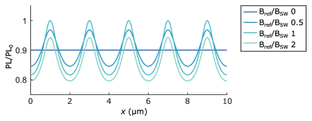
Figure S.5: Spatial profile of a single spin wave mode interfering with a reference field. The expected $\mathrm{PL}/\mathrm{PL}_{0}$ for a single spin-wave mode for various strengths of the reference field.

S.5.1 Extracting the spin wavelength of the low wavenumber mode

Here we analyze the spatial maps shown in figure 3b of the main text and extract the wavelength of the imaged modes. To do so, we first plot the signal as a function of $x$ (Fig. S.6a), after subtracting a linear term to account for the non-uniformity of the stripline-field. Using equation S.19, we then fit the averaged data (Fig. S.6a). The fit allows to extract the wavenumber $k$, which we plot as a function of $B_{0}$ (Fig. 3c, main text). In figure S.6b, we show the corresponding Fourier transform of the averaged data traces.

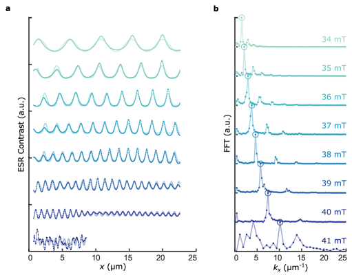
Figure S.6: Wavelength analysis of spin-wave maps (a) We average the 2D maps of figure 3b of the main text, to obtain a 1D linetrace of the ESR contrast as a function of $x$-position. We fit the data using equation S.19, to obtain the wavenumber and its uncertainty. (b) Fourier transform of the 1D data shown in (a). Circles represent peak positions used as initial guess for the fitting.

Finally, we fit the extracted wavenumbers to the backward-volume spin-wave dispersion and we find that an angle of $\theta_{B}=49$°, which is the angle between the magnetic field and the YIG surface normal, fits our data best, due to an uncertainty in mounting of the NV-probe with respect to the sample surface.

S.6 Combined atomic force microscopy and photoluminescence scans of the YIG surface

In contact mode, our scanning NV magnetometry setup collects both the topography, via the AFM feedback signal, and the NV photoluminescence (Fig. S.7). The topography image not only shows dirt particles laying on top of the surface (large white dot in the center of the scan), but also scratches and tiny pits in the YIG surface that can lead to magnon scattering [32, 33].

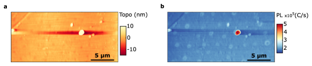
Figure S.7: YIG surface. (a) Surface topography (Topo) and (b) photoluminescence (PL) of our 235 nm-thick YIG film surface. Data corresponds to the ESR map in figure S.8b, scan 1 taken with the tip in contact with the YIG surface.

S.7 Overview spin-wave images

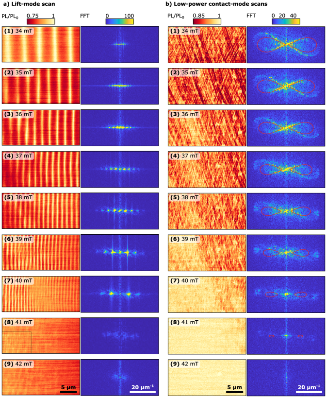
Figure S.8: Overview spin-wave images (a) Scans corresponding to Fig. 3b of the main text using $P_{\mathrm{MW}}=$4\text{\,}\mathrm{mW}$$ and we change the NV-to-sample depending on the spin-wavelength. (b) Scans corresponding to Fig. 4a of the main text using $P_{\mathrm{MW}}=$6.3\text{\,}\mathrm{\SIUnitSymbolMicro W}$$ while keeping the NV-tip in contact with the magnetic surface. Red line: the calculated isofrequency contour of the 2D spin-wave dispersion.

S.8 Calibration of the piezoelectric scanners

S.8.1 Lateral displacement

Our piezoelectric scanner (ANSxy50/LT) exhibits a nonlinear motion as a function of applied voltage. We calibrate this non-linear motion using a silicon nitride sample with $2\text{\,}\mathrm{\SIUnitSymbolMicro m}$ chess pitch structures. Specifically, we scan over the same region of interest and piezoscanner voltages/offsets while recording the photoluminescence (Figure S.9a). Our calibration procedure to convert the non-linear displacement as a function of applied voltage to position is as follows:

1. We first remove the first 25 lines from our scan data which show large non-linear and non-reproducible displacements depending on scan-speed and time spent on the first pixel.

2. We assign the applied voltage to known positions of subsequent chess pitches (Fig. S.9). For simplicity, we do this for a single row or column (Fig. S.9b).

3. We fit a second order polynomial to the known X or Y displacement.

We repeat this process for the two scan speeds used in this work: $0.1\text{\,}\mathrm{V}\text{\,}{\mathrm{s}}^{-1}$ and $0.05\text{\,}\mathrm{V}\text{\,}{\mathrm{s}}^{-1}$ used for the lift-mode and contact mode scans. We can now interpolate our 2D spatial scans, that were taken at linearly spaced voltage interval and obtain a 2D image with linearly spaced position intervals. Note that all scan data shown in the manuscript are taken in the forward scan direction and we therefore do not take piezoelectric hysteresis into account.

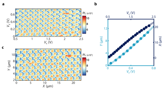
Figure S.9: Calibration of lateral piezoelectric scanners. (a) 2D spatial scan of calibration sample with a $2\text{\,}\mathrm{\SIUnitSymbolMicro m}$ pitch using linearly spaced voltage intervals at a scan speed of $0.1\text{\,}\mathrm{V}\text{\,}{\mathrm{s}}^{-1}$. (b) We fit the known X and Y-displacement of the chess pits (using a single row or column) as a function of applied X and Y voltage. (c) Interpolated data shown in (a), now using linearly spaced position intervals obtained by the fitting functions in (b) and with the first 25 scan lines removed

S.8.2 Calibration of the NV-to-sample distance

When retracting the NV-tip from the YIG surface, we observe oscillations in the NV PL (Fig. S.10a). We assume that the oscillations are caused by interference between the YIG-surface-reflected laser light and the laser light internally reflected in the diamond tip (akin to the effect leading to Newton rings). The interference leads to PL oscillations with a spatial period equal to half the laser wavelength (i.e. $515\text{\,}\mathrm{nm}$/2). We use these oscillations to estimate the tip-sample distance $d$ for each setpoint distance obtained from the linear voltage-to-distance conversion provided by the supplier of the scanners (Fig. S.10b) .

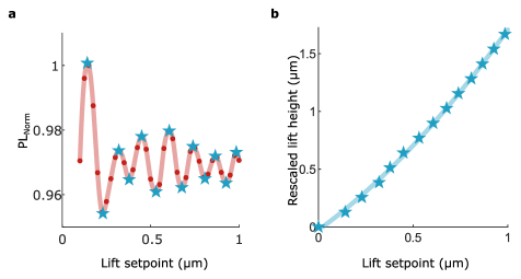
Figure S.10: Calibration of lift height. (a) Oscillating PL signal when the tip is retracted from the YIG surface. The stars are the found extrema. Data corresponds to the Rabi measurement shown in Fig. 2b of the main text. (b) We allocate a distance of $\lambda/4$ between each extremum (stars), of which the first maximum corresponds to an absolute distance of $\lambda/4$ from the surface. Our contact position is fixed at zero lift height. We use a second order polynomial to fit the displacement (solid line).

References

- [1] Sergio M Rezende “Fundamentals of magnonics” Springer, 2020
- [2] Andrii V Chumak, Alexander A Serga and Burkard Hillebrands “Magnon transistor for all-magnon data processing” In Nature Communications 5, 2014, pp. 4700
- [3] Qi Wang et al. “Reconfigurable nanoscale spin-wave directional coupler” In Science Advances 4.1, 2018, pp. e1701517 DOI: doi:10.1126/sciadv.1701517
- [4] A.. Chumak et al. “Roadmap on Spin-Wave Computing” In IEEE Transactions on Magnetics 58.6, 2022, pp. 0800172 DOI: 10.1109/TMAG.2022.3149664
- [5] LJ Cornelissen et al. “Long-distance transport of magnon spin information in a magnetic insulator at room temperature” In Nature Physics 11, 2015, pp. 1022–1026
- [6] Y. Acremann et al. “Imaging Precessional Motion of the Magnetization Vector” In Science 290.5491, 2000, pp. 492–495 DOI: doi:10.1126/science.290.5491.492
- [7] Thomas Sebastian et al. “Micro-focused Brillouin light scattering: imaging spin waves at the nanoscale” In Frontiers in Physics 3, 2015, pp. 35
- [8] Volker Sluka et al. “Emission and propagation of 1D and 2D spin waves with nanoscale wavelengths in anisotropic spin textures” In Nature Nanotechnology 14, 2019, pp. 328–333 DOI: 10.1038/s41565-019-0383-4
- [9] L. Rondin et al. “Magnetometry with nitrogen-vacancy defects in diamond” In Reports on Progress in Physics 77.5, 2014, pp. 056503 DOI: 10.1088/0034-4885/77/5/056503
- [10] C. Degen, F. Reinhard and P. Cappellaro “Quantum sensing” In Reviews of Modern Physics 89.3, 2017, pp. 035002 DOI: 10.1103/RevModPhys.89.035002
- [11] Iacopo Bertelli et al. “Magnetic resonance imaging of spin-wave transport and interference in a magnetic insulator” In Science Advances 6.46, 2020, pp. eabd3556
- [12] Aurore Finco et al. “Imaging non-collinear antiferromagnetic textures via single spin relaxometry” In Nature communications 12, 2021, pp. 767
- [13] Brendan A McCullian et al. “Broadband multi-magnon relaxometry using a quantum spin sensor for high frequency ferromagnetic dynamics sensing” In Nature Communications 11, 2020, pp. 5229
- [14] Tony X. Zhou et al. “A magnon scattering platform” In Proceedings of the National Academy of Sciences 118.25, 2021, pp. e2019473118 DOI: doi:10.1073/pnas.2019473118
- [15] Iacopo Bertelli et al. “Imaging Spin-Wave Damping Underneath Metals Using Electron Spins in Diamond” In Advanced Quantum Technologies 4.12, 2021, pp. 2100094 DOI: https://doi.org/10.1002/qute.202100094
- [16] Chunhui Du et al. “Control and local measurement of the spin chemical potential in a magnetic insulator” In Science 357.6347, 2017, pp. 195–198
- [17] Chris Koerner et al. “Frequency multiplication by collective nanoscale spin-wave dynamics” In Science 375.6585, 2022, pp. 1165–1169 DOI: doi:10.1126/science.abm6044
- [18] AA Serga, AV Chumak and B Hillebrands “YIG magnonics” In Journal of Physics D: Applied Physics 43.26, 2010, pp. 264002
- [19] Chris S Wolfe et al. “Off-resonant manipulation of spins in diamond via precessing magnetization of a proximal ferromagnet” In Physical Review B 89.18, 2014, pp. 180406(R)
- [20] Tobias Hula et al. “Nonlinear losses in magnon transport due to four-magnon scattering” In Applied Physics Letters 117.4, 2020, pp. 042404 DOI: 10.1063/5.0015269
- [21] Avinash Rustagi, Iacopo Bertelli, Toeno Van Der Sar and Pramey Upadhyaya “Sensing chiral magnetic noise via quantum impurity relaxometry” In Physical Review B 102.22, 2020, pp. 220403(R)
- [22] Paolo Andrich et al. “Long-range spin wave mediated control of defect qubits in nanodiamonds” In npj Quantum Information 3, 2017, pp. 28 DOI: 10.1038/s41534-017-0029-z
- [23] B. Flebus and Y. Tserkovnyak “Quantum-Impurity Relaxometry of Magnetization Dynamics” In Physical Review Letters 121.18, 2018, pp. 187204 DOI: 10.1103/PhysRevLett.121.187204
- [24] M. Mohseni et al. “Backscattering Immunity of Dipole-Exchange Magnetostatic Surface Spin Waves” In Physical Review Letters 122.19, 2019, pp. 197201 DOI: 10.1103/PhysRevLett.122.197201
- [25] Felix Groß et al. “Building Blocks for Magnon Optics: Emission and Conversion of Short Spin Waves” In ACS Nano 14.12, 2020, pp. 17184–17193 DOI: 10.1021/acsnano.0c07076
- [26] Joachim Gräfe et al. “Direct observation of spin-wave focusing by a Fresnel lens” In Physical Review B 102.2, 2020, pp. 024420 DOI: 10.1103/PhysRevB.102.024420
- [27] Sergej O Demokritov et al. “Bose–Einstein condensation of quasi-equilibrium magnons at room temperature under pumping” In Nature 443, 2006, pp. 430–433
- [28] Avinash Rustagi, Iacopo Bertelli, Toeno Van Der Sar and Pramey Upadhyaya “Sensing chiral magnetic noise via quantum impurity relaxometry” In Physical Review B 102.22, 2020, pp. 220403(R)
- [29] Iacopo Bertelli et al. “Magnetic resonance imaging of spin-wave transport and interference in a magnetic insulator” In Science Advances 6.46, 2020, pp. eabd3556
- [30] Tony X. Zhou et al. “A magnon scattering platform” In Proceedings of the National Academy of Sciences 118.25, 2021, pp. e2019473118 DOI: doi:10.1073/pnas.2019473118
- [31] A. Dréau et al. “Avoiding power broadening in optically detected magnetic resonance of single NV defects for enhanced dc magnetic field sensitivity” In Physical Review B 84.19, 2011, pp. 195204 DOI: 10.1103/PhysRevB.84.195204
- [32] Felix Groß et al. “Building Blocks for Magnon Optics: Emission and Conversion of Short Spin Waves” In ACS Nano 14.12, 2020, pp. 17184–17193 DOI: 10.1021/acsnano.0c07076
- [33] Joachim Gräfe et al. “Direct observation of spin-wave focusing by a Fresnel lens” In Physical Review B 102.2, 2020, pp. 024420 DOI: 10.1103/PhysRevB.102.024420