Simple and Efficient Heterogeneous Graph Neural Network

Abstract

Heterogeneous graph neural networks (HGNNs) have powerful capability to embed rich structural and semantic information of a heterogeneous graph into node representations. Existing HGNNs inherit many mechanisms from graph neural networks (GNNs) designed for homogeneous graphs, especially the attention mechanism and the multi-layer structure. These mechanisms bring excessive complexity, but seldom work studies whether they are really effective on heterogeneous graphs. In this paper, we conduct an in-depth and detailed study of these mechanisms and proposes Simple and Efficient Heterogeneous Graph Neural Network (SeHGNN). To easily capture structural information, SeHGNN pre-computes the neighbor aggregation using a light-weight mean aggregator, which reduces complexity by removing overused neighbor attention and avoiding repeated neighbor aggregation in every training epoch. To better utilize semantic information, SeHGNN adopts the single-layer structure with long metapaths to extend the receptive field, as well as a transformer-based semantic fusion module to fuse features from different metapaths. As a result, SeHGNN exhibits the characteristics of a simple network structure, high prediction accuracy, and fast training speed. Extensive experiments on five real-world heterogeneous graphs demonstrate SeHGNN’s superiority over the state-of-the-arts on both accuracy and training speed.

Introduction

Recent years witness explosive growth in graph neural networks (GNNs) in pursuit of performance improvement of graph representation learning (Wu et al. 2020; Liu et al. 2022b; Lin et al. 2022). GNNs are primarily designed for homogeneous graphs associated with a single type of nodes and edges, following a neighborhood aggregation scheme to capture structural information of a graph, where the representation of each node is computed by recursively aggregating the features of neighbor nodes (Kipf and Welling 2017).

However, GNNs are insufficient to deal with the heterogeneous graph which possesses rich semantic information in addition to structural information (Shi et al. 2016). Many real-world data in complex systems are naturally represented as heterogeneous graphs, where multiple types of entities and relations among them are embodied by various types of nodes and edges, respectively. For example, as shown in Figure 1, the citation network ACM includes several types of nodes: Paper (P), Author (A), and Subject (S), as well as many relations with different semantic meanings, such as Author$\xrightarrow{\rm writes}$Paper, Paper$\xrightarrow{\rm cites}$Paper, Paper$\xrightarrow{\rm belongs~{}to}$Subject. These relations can be composited with each other to form high-level semantic relations, which are represented as metapaths (Sun et al. 2011; Sun and Han 2012). For example, the 2-hop metapath Author-Paper-Author (APA) represents the co-author relationship, while the 4-hop metapath Author-Paper-Subject-Paper-Author (APSPA) describes that the two authors have been engaged in the research of the same subject. Heterogeneous graphs contain more comprehensive information and rich semantics and require specifically designed models.

Various heterogeneous graph neural networks (HGNNs) have been proposed to capture semantic information, achieving great performance in heterogeneous graph representation learning (Dong et al. 2020; Yang et al. 2020; Wang et al. 2020; Zheng et al. 2022; Yan et al. 2022). Therefore, HGNNs are at the heart of a broad range of applications such as social network analysis (Liu et al. 2018), recommendation (Fan et al. 2019; Niu et al. 2020), and knowledge graph inference (Bansal et al. 2019; Vashishth et al. 2020; Wang et al. 2021a).

Figure 1 depicts the two main categories of HGNNs. Metapath-based methods (Schlichtkrull et al. 2018; Zhang et al. 2019; Wang et al. 2019; Fu et al. 2020) capture the structural information of the same semantic first and then fuse different semantic information. These models first aggregate neighbor features at the scope of each metapath to generate semantic vectors, and then fuse these semantic vectors to generate the final embedding vector. Metapath-free methods (Zhu et al. 2019; Hong et al. 2020; Hu et al. 2020b; Lv et al. 2021) capture structural and semantic information simultaneously. These models aggregate messages from a node’s local neighborhood like traditional GNNs, but use extra modules (e.g. attentions) to embed semantic information such as node types and edge types into propagated messages.

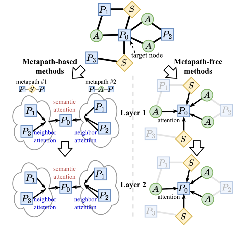
Figure 1: The general architectures of metapath-based methods and metapath-free methods on heterogeneous graphs.

Existing HGNNs inherit many mechanisms from GNNs over homogeneous graphs, especially the attention mechanism and the multi-layer structure, as illustrated in Figure 1, but seldom work studies whether these mechanisms are really effective on heterogeneous graphs. Moreover, the hierarchy attention calculation in the multi-layer network and repeated neighbor aggregation in every epoch bring excessive complexity and computation. For example, the neighbor aggregation process with attention modules takes more than 85% of total time in the metapath-based model HAN (Wang et al. 2019) and the metapath-free model HGB (Lv et al. 2021), which has become the speed bottleneck for the application of HGNNs on larger-scale heterogeneous graphs.

This paper provides an in-depth and detailed study of these mechanisms and yields two findings: (1) semantic attention is essential while neighbor attention is not necessary, (2) models with a single-layer structure and long metapaths outperform those with multi-layers and short metapaths. These findings imply that neighbor attention and multi-layer structure not only introduce unnecessary complexity, but also hinder models to from achieving better performance.

To this end, we propose a novel metapath-based method named SeHGNN. SeHGNN employs the mean aggregator (Hamilton, Ying, and Leskovec 2017) to simplify neighbor aggregation, adopts a single-layer structure with long metapaths to extend the receptive field, and utilizes a transformer-based semantic fusion module to learn mutual attentions between semantic pairs. Additionally, as the simplified neighbor aggregation in SeHGNN is parameter-free and only involves linear operations, it earns the opportunity to execute the neighbor aggregation in the pre-processing step only once. As a result, SeHGNN not only demonstrates better performance but also avoids the need of repeated neighbor aggregation in every training epoch, leading to significant improvements in training speed.

We conduct experiments on four widely-used datasets from HGB benchmark (Lv et al. 2021) and a large-scale dataset from OGB challenge (Hu et al. 2020a). Results show that SeHGNN achieves superior performance over the state-of-the-arts for node classification on heterogeneous graphs.

The contributions of this work are summarized as follows:

• We conduct an in-depth study about the attention mechanism and the network structure in HGNNs and obtain two important findings, which reveal the needlessness of neighbor attention and the superiority of utilizing the single-layer structure and long metapaths.

• Motivated by the findings above, we propose a simple and effective HGNN architecture SeHGNN. To easily capture structural information, SeHGNN pre-computes the neighbor aggregation in the pre-processing step using a light-weight mean aggregator, which removes the overused neighbor attention and avoids repeated neighbor aggregation in every training epoch. To better utilize semantic information, SeHGNN adopts the single-layer structure with long metapaths to extend the receptive field, as well as a transformer-based semantic fusion module to fuse features from different metapaths.

• Experiments on five widely-used datasets demonstrate the superiority of SeHGNN over the state-of-the-arts, i.e., high prediction accuracy and fast training speed.

Preliminaries

Definition 1   Heterogeneous graphs.  A heterogeneous graph is defined as $G=\{V,E,\mathcal{T}^{v},\mathcal{T}^{e}\}$, where $V$ is the set of nodes with a node type mapping function $\phi:V\rightarrow\mathcal{T}^{v}$, and $E$ is the set of edges with an edge type mapping function $\psi:E\rightarrow\mathcal{T}^{e}$. Each node $v_{i}{\in}V$ is attached with a node type $c_{i}{=}\phi(v_{i}){\in}\mathcal{T}^{v}$. Each edge $e_{t\leftarrow s}{\in}E\,$($e_{ts}$ for short) is attached with a relation $r_{c_{t}\leftarrow c_{s}}{=}\psi(e_{ts}){\in}\mathcal{T}^{e}$ ($r_{c_{t}c_{s}}$ for short), pointing from the source node $s$ to the target node $t$. When $|\mathcal{T}^{v}|{=}|\mathcal{T}^{e}|{=}1$, the graph degenerates into homogeneous.

The graph structure of $G$ can be represented by a series of adjacency matrices $\{A_{r}:r\in\mathcal{T}^{e}\}$. For each relation $r_{c_{t}c_{s}}{\in}\mathcal{T}^{e}$,  $A_{c_{t}c_{s}}{\in}\mathbb{R}^{|V^{c_{t}}|\times|V^{c_{s}}|}$ is the corresponding adjacency matrix where the nonzero values indicate positions of edges $E^{c_{t}c_{s}}$ of the current relation.

Definition 2   Metapaths.  A metapath defines a composite relation of several edge types, represented as $\mathcal{P}\triangleq c_{1}\leftarrow c_{2}\leftarrow\ldots\leftarrow c_{l}$  ($\mathcal{P}=c_{1}c_{2}\ldots c_{l}$ for short).

Given the metapath $\mathcal{P}$, a metapath instance $p$ is a node sequence following the schema defined by $\mathcal{P}$, represented as $p(v_{1},v_{l})=\{v_{1},\,e_{12},\,v_{2},\,\ldots,\,v_{l-1},\,e_{(l-1)l},\,v_{l}:v_{i}\in V^{c_{i}},\,e_{i(i+1)}\in E^{c_{i}c_{i+1}}\}$. In particular, $p(v_{1},v_{l})$ indicates the relationship of $(l{-}1)$-hop neighborhood where $v_{1}$ is the target node and $v_{l}$ is one of $v_{1}$’s metapath-based neighbors.

Given a metapath $\mathcal{P}$ with the node types of its two ends as $c_{1},c_{l}$, a metapath neighbor graph $G^{\mathcal{P}}=\{V^{c_{1}}\bigcup V^{c_{l}},E^{\mathcal{P}}\}$ can be constructed out of $G$, where an edge $e_{ij}\in E^{\mathcal{P}},\phi(i)=c_{1},\phi(j)=c_{l}$ exists in $G^{\mathcal{P}}$ if and only if there is an metapath instance $p(v_{i},v_{j})$ of $\mathcal{P}$ in $G$.

Related Work

For homogeneous graphs, GNNs are widely used to learn node representation from the graph structure. The pioneer GCN (Kipf and Welling 2017) proposes a multi-layer network following a layer-wise propagation rule, where the $l^{th}$ layer learns an embedding vector $h_{v}^{(l+1)}$ by aggregating features $\{h_{u}^{(l)}:u\in\mathcal{N}_{v}\}$ from the local 1-hop neighbor set $\mathcal{N}_{v}$ for each node $v\in V$. GraphSAGE (Hamilton, Ying, and Leskovec 2017) improves the scalability for large graphs by introducing mini-batch training and neighbor sampling (Liu et al. 2022a). GAT (Veličković et al. 2018) introduces the attention mechanism to encourage the model to focus on the most important part of neighbors. SGC (Wu et al. 2019) removes nonlinearities between consecutive graph convolutional layers, which brings great acceleration and does not impact model effects.

Heterogeneous graphs contain rich semantics besides structural information, revealed by multiple types of nodes and edges. According to the way to deal with different semantics, HGNNs are categorized into metapath-based and metapath-free methods.

Metapath-based HGNNs first aggregate neighbor features of the same semantic and then fuse different semantics. RGCN (Schlichtkrull et al. 2018) is the first to separate 1-hop neighbor aggregation according to edge types. HetGNN (Zhang et al. 2019) takes use of neighbors of different hops. It uses random walks to collect neighbors of different distances and then aggregates neighbors of the same node type. HAN (Wang et al. 2019) utilizes metapaths to distinguish different semantics. It aggregates structural information with neighbor attention in each metapath neighbor graph in the neighbor aggregation step, and then fuses outputs from different subgraphs with semantic attention for each node in the semantic fusion step. MAGNN (Fu et al. 2020) further leverages all nodes in a metapath instance rather than only the nodes of the two endpoints.

Metapath-free HGNNs aggregate messages from neighbors of all node types simultaneously within the local 1-hop neighborhood like GNNs, but using additional modules such as attentions to embed semantic information such as node types and edge types into propagated messages. RSHN (Zhu et al. 2019) builds the coarsened line graph to obtain the global embedding representation of different edge types, and then it uses the combination of neighbor features and edge-type embeddings for feature aggregation in each layer. HetSANN (Hong et al. 2020) uses a multi-layer GAT network with type-specific score functions to generate attentions for different relations. HGT (Hu et al. 2020b) proposes a novel heterogeneous mutual attention mechanism based on Transformer (Vaswani et al. 2017), using type-specific trainable parameters for different types of nodes and edges. HGB (Lv et al. 2021) takes the multi-layer GAT network as the backbone and incorporates both node features and learnable edge-type embeddings to generate attention values.

	DBLP		ACM
	macro-f1	micro-f1	macro-f1	micro-f1
HAN	92.59	93.06	90.30	90.15
HAN*	92.75	93.23	90.61	90.48
HAN†	92.19	92.66	89.78	89.67
HGB	94.15	94.53	93.09	93.03
HGB*	94.20	94.58	93.11	93.05
HGB†	93.77	94.15	92.32	92.27

Table 1: Experiments to analyze the effects of two kinds of attentions. * means removing neighbor attention and $\dagger$ means removing semantic attention.

	DBLP		ACM
network	macro-f1	micro-f1	macro-f1	micro-f1
(1,)	79.43	80.16	89.81	90.03
(1,1)	85.06	86.69	90.79	90.87
(2,)	88.18	88.83	91.64	91.67
(1,1,1)	88.38	89.37	87.95	88.84
(3,)	93.33	93.72	92.67	92.64
(1,1,1,1)	89.55	90.44	88.62	88.93
(2,2)	91.88	92.35	92.57	92.53
(4)	93.60	94.02	92.82	92.79

Table 2: Experiments to analyze the effects of different combinations of the number of layers and the maximum metapath hop. e.g., the structure (1,1,1) means a three-layer network with all metapaths no more than 1 hop in each layer.

Except for the above two main categories of HGNNs, SGC-based work such as NARS (Yu et al. 2020), SAGN (Sun, Gu, and Hu 2021), and GAMLP (Zhang et al. 2022) also show impressive results on heterogeneous graphs, but they aggregate features of all types of nodes together without explicitly distinguishing different semantics.

Motivation

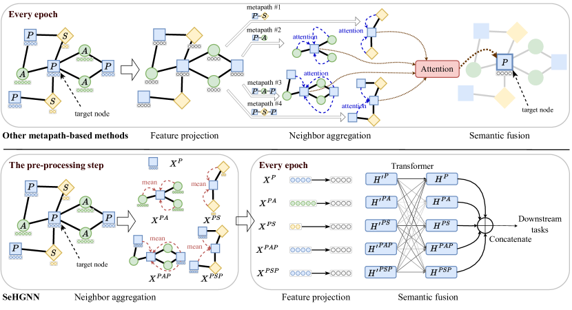
Figure 2: The architecture of SeHGNN compared to previous metapath-based methods. The example is based on ACM dataset with node types author (A), paper (P), and subject (S). This figure exhibits aggregation of 0-hop metapath P (the target node itself), 1-hop metapaths PA, PS, and 2-hop metapaths PAP, PSP.

Existing HGNNs inherit many mechanisms from GNNs without analysis of their effects. In this section, we conduct an in-depth and detailed study of widely-used mechanisms, i.e. the attention mechanism and the multi-layer structure for HGNNs. Through experiments, we obtain two important findings that guide us in designing the architecture of SeHGNN. All results presented in this section are the average of 20 runs with different data partitions to mitigate the influence of random noise.

Study on attentions. HGNNs use multiple attentions, as shown in Figure 1, which are calculated using distinct modules or parameters. These attentions can be classified into two types: neighbor attention within neighbors of the same relation and semantic attention among different relations. Metapath-based methods like HAN incorporate two attentions in the neighbor aggregation step and the semantic fusion step, respectively. Metapath-free methods like HGB compute attentions of 1-hop neighbors with relation-specific embeddings. While distinguishing between the two types of attention in metapath-free methods can be challenging, we can perform additional calculations to eliminate the influence of either attention. Specifically, for the attentions values of each node’s neighbors, we can average them within each relation which equals removing neighbor attention, or normalize them within each relation so that each relation contributes equally to final results to remove semantic attention.

Re-implement experiments on HGB reveal that a well-trained HGB model tends to assign similar attention values within each relation, leading us to investigate the necessity of different attentions. We conduct experiments on HAN and HGB, where * means removing neighbor attention and ^† means removing semantic attention. Results in Table 1 indicate that models without semantic attention exhibit a decrease of model effects, while models without neighbor attention do not, from which we obtain the first finding.

Finding 1: Semantic attention is essential, while neighbor attention is not necessary. This finding is reasonable, as semantic attention is able to weigh the importance of different semantics. And for neighbor attention, various SGC-based work (Wu et al. 2019; Rossi et al. 2020; Zhang et al. 2022) has demonstrated that simple mean aggregation can be just as effective as aggregation with attention modules.

Study on multi-layer structure. Without neighbor attention, metapath-free methods have an equivalent form that first averages features of neighbors within each relation and then fuses outputs of different relations. Therefore, they can be converted to metapath-based methods with a multi-layer structure and only 1-hop metapaths in each layer. So, in the following experiments, we focus on the influence of number of layers and metapaths in metapath-based methods.

We conduct experiments on HAN using a list of numbers to represent the structure of each variant. For instance, on the ACM dataset, the structure (1,1,1,1) represents a four-layer network with 1-hop metapaths PA, PS in each layer, and (4) represent a single-layer network with all metapaths no more than 4-hop, such as PA, PS, PAP, PSP, PAPAP, PSPSP and so on. These lists also exhibit the sizes of receptive field. For example, structures (1,1,1,1), (2,2), (4) have the same receptive field size, which involves 4-hop neighbors. Based on the results shown in Table 2, we conclude the second finding.

Finding 2: Models with a single-layer structure and long metapaths outperform those with multi-layers and short metapaths. As shown in Table 2, models with a single-layer and long metapaths achieve better performance under the same size of the receptive field. We attribute this to the fact that multi-layer networks fuse semantics per layer, making it difficult to distinguish high-level semantics. For instance, in a model with the structure (4), the utilization of multi-hop metapaths allow us to distinguish between high-level semantics, such as being written by the same author (PAP) or familiar authors (PAPAP), whereas these distinctions are unavailable in a four-layer network (1,1,1,1) as all intermediate vectors between two consecutive layers represent mixtures of different semantics. Moreover, increasing the maximum metapath length enhances the model’s performance by introducing more metapaths with different semantics.

Proposal of SeHGNN. Motivated by the two findings, on one hand, we can avoid redundant neighbor attention by employing mean aggregation at the scope of each metapath without sacrificing model effects; on the other hand, we can simplify the network structure using a single layer, but use more and longer metapaths to expand the receptive field and achieve better performance. Furthermore, as the neighbor aggregation part without the attention module involves only linear operations and no trainable parameters, it endows an opportunity to execute neighbor aggregation in the pre-processing step only once rather than in every training epoch, which significantly reduces the training time. Overall, these optimizations simplify the network structure and make it more efficient, which are the key points of SeHGNN.

Methodology

This section formally proposes Simple and Efficient Heterogeneous Neural Network (SeHGNN). SeHGNN’s architecture is illustrated in Figure 2 and includes three primary components: simplified neighbor aggregation, multi-layer feature projection, and transformer-based semantic fusion. Figure 2 also highlights the distinction between SeHGNN and other metapath-based HGNNs, i.e., SeHGNN pre-computes the neighbor aggregation in the pre-processing step, thereby avoiding the excessive complexity of repeated neighbor aggregation in every training epoch. Algorithm 1 outlines the overall training process.

Simplified Neighbor Aggregation

The simplified neighbor aggregation is executed only once in the pre-processing step and generates a list of feature matrices $M=\{X^{\mathcal{P}}:\mathcal{P}\in\Phi_{X}\}$ of different semantics for the set $\Phi_{X}$ of all given metapaths. Generally, for each node $v_{i}$, it employs the mean aggregation to aggregate features from metapath-based neighbors for each given metapath, and outputs a list of semantic feature vectors, denoted as

$$m_{i}=\{\mathbf{z}^{\mathcal{P}}_{i}=\frac{1}{||S^{\mathcal{P}}||}\sum_{p(i,j)\in S_{\mathcal{P}}}\mathbf{x}_{j}:\mathcal{P}\in\Phi_{X}\},$$

where $S^{\mathcal{P}}$ is the set of all metapath instances corresponding to metapath $\mathcal{P}$ and $p(i,j)$ represents one metapath instance with the target node $i$ and the source node $j$.

We propose a new method to simplify the collection of metapath-based neighbors. Existing metapath-based methods like HAN build metapath neighbor graphs that enumerate all metapath-based neighbors for each metapath, which brings a high overhead as the number of metapath instances grows exponentially with the length of the metapath. Inspired by the layer-wise propagation of GCN, we calculate the final contribution weight of each node to targets using the multiplication of adjacency matrices. Specifically, let $X^{c}=\{{x_{0}^{c}}^{T};{x_{1}^{c}}^{T};$ $\ldots;{x_{||V^{c}||-1}^{c}}^{T}\}\in\mathbb{R}^{||V^{c}||\times d^{c}}$ be the raw feature matrix of all nodes belonging to type $c$, where $d^{c}$ is the feature dimension, and then the simplified neighbor aggregation process can be expressed as

$$X^{\mathcal{P}}=\hat{A}_{c,c_{1}}\hat{A}_{c_{1},c_{2}}\ldots\hat{A}_{c_{l-1},c_{l}}X^{c_{l}},$$

where $\mathcal{P}=cc_{1}c_{2}\ldots c_{l}$ is a $l$-hop metapath, and $\hat{A}_{c_{i},c_{i+1}}$ is the row-normalized form of adjacency matrix $A_{c_{i},c_{i+1}}$ between node type $c_{i}$ and $c_{i+1}$. Please note that, the aggregation results of short metapaths can be used as intermediate values for long metapaths. For example, given two metapaths PAP and PPAP for the ACM dataset, we can calculate $X^{PAP}$ first and then calculate $X^{PPAP}=\hat{A}_{PP}X^{PAP}$.

Algorithm 1 The overall training process of SeHGNN

Input: Raw feature matrices $\{X^{c_{i}}:c_{i}\in\mathcal{T}^{v}\}$; the raw label matrix $Y$; metapath sets $\Phi_{X}$ for features and $\Phi_{Y}$ for labels
Parameter: ${\rm MLP}_{\mathcal{P}_{i}}$ for feature projection; $W_{Q}$, $W_{K}$, $W_{V}$, $\beta$ for semantic fusion; ${\rm MLP}$ for downstream tasks
Output: Node classification results ${\rm Pred}$ for target type $c$

1:  % Neighbor aggregation

2:  Calculate aggregation of raw features for each $\mathcal{P}\in\Phi_{X}$ $X^{\mathcal{P}}{=}\hat{A}_{c,c_{1}}\ldots\hat{A}_{c_{l{-}1}c_{l}}X^{c_{l}},\,\,\,\,\mathcal{P}{=}cc_{1}\ldots c_{l{-}1}c_{l}$

3:  Calculate aggregation of labels for each $\mathcal{P}\in\Phi_{Y}$ $Y^{\mathcal{P}}{=}{\rm rm\_diag}(\hat{A}_{c,c_{1}}\ldots\hat{A}_{c_{l{-}1}c})Y,\,\,\,\,\mathcal{P}{=}cc_{1}\ldots c_{l{-}1}c$

4:  Collect all semantic matrices $M=\{X^{\mathcal{P}}:\mathcal{P}\in\Phi_{X}\}\bigcup\{Y^{\mathcal{P}}:\mathcal{P}\in\Phi_{Y}\}$

5:  for ${\rm each\,epoch}$ do

6:     % Feature projection

7:     ${H^{\prime}}^{\mathcal{P}_{i}}={\rm MLP}_{\mathcal{P}_{i}}(M^{\mathcal{P}_{i}}),\,\,M^{\mathcal{P}_{i}}\in M$

8:     % Semantic fusion

9:     $Q^{\mathcal{P}_{i}}{=}W_{Q}{H^{\prime}}^{\mathcal{P}_{i}},\,K^{\mathcal{P}_{i}}{=}W_{K}{H^{\prime}}^{\mathcal{P}_{i}},\,V^{\mathcal{P}_{i}}{=}W_{V}{H^{\prime}}^{\mathcal{P}_{i}}$

10:     $\alpha_{ij}=\frac{\exp{(Q^{\mathcal{P}_{i}}\cdot{K^{\mathcal{P}_{j}}}^{T}})}{\sum_{t}\exp{(Q^{\mathcal{P}_{i}}\cdot{K^{\mathcal{P}_{t}}}^{T})}}$

11:     $H^{\mathcal{P}_{i}}=\beta\sum_{j}\alpha_{ij}V^{\mathcal{P}_{i}}+{H^{\prime}}^{\mathcal{P}_{i}}$

12:     $H^{c}={\rm concatenate}([H^{\mathcal{P}_{1}}||H^{\mathcal{P}_{2}}||\ldots])$

13:     % Downstream tasks

14:     ${\rm Pred}={\rm MLP}(H^{c})$

15:     Calculate loss function $\mathcal{L}=-\sum_{i}y_{i}\ln pred_{i}$, do back-propagation and update network parameters

16:  end for

17:  return ${\rm Pred}$

Besides, previous (Wang and Leskovec 2020; Wang et al. 2021b; Shi et al. 2021) research has demonstrated that incorporating labels as additional inputs can improve model performance. To capitalize on this, similar to the aggregation of raw features, we represent labels in the one-hot format and propagate them across various metapaths. This process generates a series of matrices $\{Y^{\mathcal{P}}:\mathcal{P}\in\Phi_{Y}\}$ that reflect the label distribution of corresponding metapath neighbor graphs. Please note that the two endpoints of any metapath $\mathcal{P}\in\Phi_{Y}$ should be the target node type $c$ in the node classification task. Given a metapath $\mathcal{P}=cc_{1}c_{2}\ldots c_{l-1}c\in\Phi_{Y}$, the label propagation process can be represented as

$$Y^{\mathcal{P}}={\rm rm\_diag}(\hat{A}^{\mathcal{P}})Y^{c},\,\hat{A}^{\mathcal{P}}=\hat{A}_{c,c_{1}}\hat{A}_{c_{1},c_{2}}\ldots\hat{A}_{c_{l-1},c},$$

where $Y^{c}$ is the raw label matrix. In the matrix $Y^{c}$, rows corresponding to nodes in the training set take the values of one-hot format labels, while other rows are filled with 0. To avoid label leakage, we prevent each node from receiving the ground truth label information of itself, by removing the diagonal values in the results of multiplication of adjacency matrices. The label propagation also executes in the neighbor aggregation step and produces semantic matrices as extra inputs for later training.

		DBLP		IMDB		ACM		Freebase
		macro-f1	micro-f1	macro-f1	micro-f1	macro-f1	micro-f1	macro-f1	micro-f1
1st	RGCN	91.52±0.50	92.07±0.50	58.85±0.26	62.05±0.15	91.55±0.74	91.41±0.75	46.78±0.77	58.33±1.57
	HetGNN	91.76±0.43	92.33±0.41	48.25±0.67	51.16±0.65	85.91±0.25	86.05±0.25	-	-
	HAN	91.67±0.49	92.05±0.62	57.74±0.96	64.63±0.58	90.89±0.43	90.79±0.43	21.31±1.68	54.77±1.40
	MAGNN	93.28±0.51	93.76±0.45	56.49±3.20	64.67±1.67	90.88±0.64	90.77±0.65	-	-
2nd	RSHN	93.34±0.58	93.81±0.55	59.85±3.21	64.22±1.03	90.50±1.51	90.32±1.54	-	-
	HetSANN	78.55±2.42	80.56±1.50	49.47±1.21	57.68±0.44	90.02±0.35	89.91±0.37	-	-
	HGT	93.01±0.23	93.49±0.25	63.00±1.19	67.20±0.57	91.12±0.76	91.00±0.76	29.28±2.52	60.51±1.16
	HGB	94.01±0.24	94.46±0.22	63.53±1.36	67.36±0.57	93.42±0.44	93.35±0.45	47.72±1.48	66.29±0.45
3rd	SeHGNN	95.06±0.17	95.42±0.17	67.11±0.25	69.17±0.43	94.05±0.35	93.98±0.36	51.87±0.86	65.08±0.66
4th	Variant#1	93.61±0.51	94.08±0.48	64.48±0.45	66.58±0.42	93.06±0.18	92.98±0.18	33.23±1.39	57.60±1.17
	Variant#2	94.66±0.27	95.01±0.24	65.27±0.60	66.68±0.52	93.46±0.43	93.38±0.44	46.82±1.12	64.08±1.43
	Variant#3	94.86±0.14	95.24±0.13	66.63±0.34	68.21±0.32	93.95±0.48	93.87±0.50	50.71±0.44	63.41±0.47
	Variant#4	94.52±0.05	94.93±0.06	64.99±0.54	66.65±0.50	93.88±0.63	93.80±0.64	50.30±0.23	64.53±0.38

Table 3: Experiment results on the four datasets from HGB benchmark, where “-” means that the models run out of memory.

Multi-layer Feature Projection

The feature projection step projects semantic vectors into the same data space, as semantic vectors of different metapaths may have different dimensions or lie in various data spaces. Generally, it defines a semantic-specific transformation matrix $W^{\mathcal{P}}$ for each metapath $\mathcal{P}$ and calculates ${H^{\prime}}^{\mathcal{P}}=W^{\mathcal{P}}X^{\mathcal{P}}$. For better representation power, we use a multi-layer perception block $\rm{MLP}_{\mathcal{P}}$ for each metapath $\mathcal{P}$ with a normalization layer, a nonlinear layer, and a dropout layer between two consecutive linear layers. Then, this process can be expressed as

$${H^{\prime}}^{\mathcal{P}}=\rm{MLP}_{\mathcal{P}}(X^{\mathcal{P}}).$$

Transformer-based Semantic Fusion

The semantic fusion step fuses semantic feature vectors and generates the final embedding vector for each node. Rather than using a simple weighted sum format, we propose a transformer (Vaswani et al. 2017) -based semantic fusion module to further explore the mutual relationship between each pair of semantics.

The transformer-based semantic fusion module is designed to learn the mutual attention between pairs of semantic vectors, given the pre-defined metapath list $\Phi=\{\mathcal{P}_{1},\ldots,\mathcal{P}_{K}\}$ and projected semantic vectors $\{{h^{\prime}}^{\mathcal{P}_{1}},\ldots,{h^{\prime}}^{\mathcal{P}_{K}}\}$ for each node. For each semantic vector ${h^{\prime}}^{\mathcal{P}_{i}}$, the module maps this vector into a query vector $q^{\mathcal{P}_{i}}$, a key vector $k^{\mathcal{P}_{i}}$, and a value vector $v^{\mathcal{P}_{i}}$. The mutual attention weight $\alpha_{(\mathcal{P}_{i},\mathcal{P}_{j})}$ is the dot product result of the query vector $q^{\mathcal{P}_{i}}$ and the key vector $k^{\mathcal{P}_{j}}$ after a softmax normalization. The output vector $h^{\mathcal{P}_{i}}$ of current semantic $\mathcal{P}_{i}$ is the weighted sum of all value vectors $v^{\mathcal{P}_{j}}$ plus a residual connection. The process of semantic fusion can be presented as

$$q^{\mathcal{P}_{i}}=W_{Q}{h^{\prime}}^{\mathcal{P}_{i}},\,k^{\mathcal{P}_{i}}=W_{K}{h^{\prime}}^{\mathcal{P}_{i}},\,v^{\mathcal{P}_{i}}=W_{V}{h^{\prime}}^{\mathcal{P}_{i}},\,\,\mathcal{P}_{i}\in\Phi,$$

$$\alpha_{(\mathcal{P}_{i},\mathcal{P}_{j})}=\frac{\exp{(q^{\mathcal{P}_{i}}\cdot{k^{\mathcal{P}_{j}}}^{T})}}{\sum_{\mathcal{P}_{t}\in\Phi}\exp{(q^{\mathcal{P}_{i}}\cdot{k^{\mathcal{P}_{t}}}^{T})}},$$

$$h^{\mathcal{P}_{i}}=\beta\sum_{\mathcal{P}_{j}\in\Phi}\alpha_{(\mathcal{P}_{i},\mathcal{P}_{j})}\,v^{\mathcal{P}_{j}}+{h^{\prime}}^{\mathcal{P}_{i}},$$

where $W_{Q},W_{K},W_{V},\beta$ are trainable parameters shared across all metapaths.

The final embedding vector of each node is the concatenation of all those output vectors. For downstream tasks like the node classification, another MLP is used to generate prediction results, which can be expressed as

$${\rm Pred}={\rm MLP}([h^{\mathcal{P}_{1}}||h^{\mathcal{P}_{2}}||\ldots||h^{\mathcal{P}_{|\Phi|}}]).$$

Experiment

Experiments are conducted on four widely-used heterogeneous graphs including DBLP, ACM, IMDB, and Freebase from HGB benchmark (Lv et al. 2021), as well as a large-scale dataset ogbn-mag from OGB challenge (Hu et al. 2021). The details about all experiment settings and the network configurations are recorded in Appendix.

Results on HGB Benchmark

Table 3 presents the performance of SeHGNN on four datasets compared to several baselines in HGB benchmark, including four metapath-based methods (1st block) and four metapath-free methods (2nd block). Results demonstrate the effectiveness of SeHGNN as it achieves the best performance over all these baselines but the second best for micro-f1 accuracy on the Freebase dataset.

Additionally, we conduct comprehensive ablation studies to validate the two findings in the Motivation section and to determine the importance of other modules. The 4th block of Table 3 shows the results of four variants of SeHGNN.

Variant#1 utilizes GAT for each metapath in the neighbor aggregation step like HAN. Variant#2 uses a two-layer structure, where each layer has independent neighbor aggregation and semantic fusion steps, but the maximum hop of metapaths in each layer is half of that in SeHGNN to ensure that SeHGNN and its Variant#2 have the same size of receptive field. The performance gap between SeHGNN and its two variants proves that the two findings also apply for SeHGNN.

Variant#3 does not include labels as extra inputs, and Variant#4 replaces the transformer-based semantic fusion with the weighted sum fusion like HAN. Notably, although inferior to SeHGNN, Variant#3 has already outperformed most baselines except the micro-f1 on the Freebase dataset. These results show that the utilization of label propagation and transformer-based fusion improves model performance.

Methods	Validation accuracy	Test accuracy
RGCN	48.35±0.36	47.37±0.48
HGT	49.89±0.47	49.27±0.61
NARS	51.85±0.08	50.88±0.12
SAGN	52.25±0.30	51.17±0.32
GAMLP	53.23±0.23	51.63±0.22
HGT+emb	51.24±0.46	49.82±0.13
NARS+emb	53.72±0.09	52.40±0.16
GAMLP+emb	55.48±0.08	53.96±0.18
SAGN+emb+ms	55.91±0.17	54.40±0.15
GAMLP+emb+ms	57.02±0.41	55.90±0.27
SeHGNN	55.95±0.11	53.99±0.18
SeHGNN+emb	56.56±0.07	54.78±0.17
SeHGNN+ms	58.70±0.08	56.71±0.14
SeHGNN+emb+ms	59.17±0.09	57.19±0.12

Table 4: Experiment results on ogbn-mag compared with methods on the OGB leaderboard, where “emb” means using extra embeddings and “ms” means multi-stage training.

Results on Ogbn-mag

The ogbn-mag dataset presents two extra challenges: (1) some types of nodes lack raw features, (2) target type nodes are split according to years, causing training nodes and test nodes to have different data distribution. Existing methods usually address these challenges by (1) generating extra embeddings (abbreviated as emb) using unsupervised representation learning algorithms like ComplEx (Trouillon et al. 2016) and (2) utilizing multi-stage learning (abbreviated as ms), which selects test nodes with confident predictions in last training stage, adds these nodes to the training set and re-trains the model in the new stage (Li, Han, and Wu 2018; Sun, Lin, and Zhu 2020; Yang et al. 2021). To provide a comprehensive comparison, we compare results with or without these tricks. For methods without emb, we use randomly initialized raw feature vectors.

Table 4 displays the results on the large-scale dataset ogbn-mag compared with baselines on the OGB leaderboard. Results show that SeHGNN outperforms other methods under the same condition. It is worth noting that SeHGNN with randomly initialized features even outperforms others with well-trained embeddings from additional representation learning algorithms, which reflects that SeHGNN learns more information from the graph structure.

Time Analysis

Firstly, we theoretically analyze the time complexity of SeHGNN compared to HAN and HGB as Table 5 shows. We assume a one-layer structure with $k$ metapaths for SeHGNN and HAN, and $l$-layer structure for HGB. The maximum hop of metapaths is also $l$ to ensure the same size of receptive field. The number of target type nodes is $n$ and the dimension of input and hidden vectors is $d$. The average number of neighbors in metapath neighbor graphs on HAN and involved neighbors during multi-layer aggregation on HGB are $e_{1},e_{2}$, respectively. Please note that both $e_{1}$ and $e_{2}$ grow exponentially with the length of metapaths and layer number $l$. For the above five datasets we use tens of metapaths at most, but each node averagely aggregates information from thousands of neighbors for $l\geq 3$. Generally, we have $e_{1}\gg k^{2},e_{2}\gg k^{2}$, so the theoretical complexity of SeHGNN is much lower than that of HAN and HGB.

To validate our theoretical analysis, we conduct experiments to compare the time consumption of SeHGNN with previous HGNNs. Figure 3 shows achieving micro-f1 scores relative to the average time consumption of each training epoch for these models, which reflects the superiority of SeHGNN on both the training speed and the model effect.

	Feature projection	Neighbor    aggregation	Semantic fusion	Total
SeHGNN	$\,\,O(nkd^{2})$	–	$O(n(kd^{2}{+}k^{2}d))$	$\,\,O(nd(k^{2}{+}kd))$
HAN	$O(nd^{2})$	$O(nke_{1}d)$	$O(nkd^{2})$	$O(nd(ke_{1}{+}kd))$
HGB	$O(nld^{2})$	$O(ne_{2}d)$		$O(nd(e_{2}{+}ld))$

Table 5: Time complexity of SeHGNN, HAN and HGB.

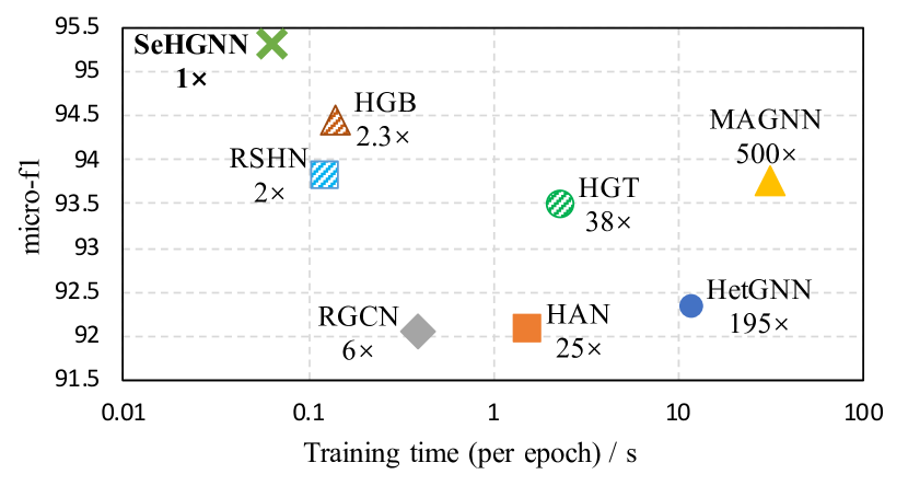
Figure 3: Micro-f1 scores and time consumption of different HGNNs on DBLP dataset. Numbers below model names exhibit the ratio of time consumption relative to SeHGNN. e.g., “6x” below RGCN means RGCN costs 6 times of time.

Conclusion

This paper proposes a novel approach called SeHGNN for heterogeneous graph representation learning, which is based on two key findings about attention utilization and network structure. SeHGNN adopts a light-weight mean aggregator to pre-compute neighbor aggregation, which effectively captures structural information while avoiding overused neighbor attention and repeated neighbor aggregation. Moreover, SeHGNN utilizes a single-layer structure with long metapaths to extend the receptive field and a transformer-based semantic fusion module to better utilize semantic information, resulting in significant improvements in model effectiveness. Experiments on five commonly used datasets demonstrate that SeHGNN outperforms state-of-the-art methods in terms of both accuracy and training speed.

Appendix A Appendix

Observation in HGB models

The metapath-free method HGB (Lv et al. 2021) calculates the attention value over each edge using the concatenation of node embeddings of the two endpoints and the edge-type embedding, presented as

$$\alpha_{ij}=\frac{{\rm exp}({\rm LeakyReLU}(\mathbf{a}^{T}[\mathbf{Wh}_{i}||\mathbf{Wh}_{j}||\mathbf{W}_{r}\mathbf{r}_{ij}]))}{\sum_{k\in\mathcal{N}_{i}}{\rm exp}({\rm LeakyReLU}(\mathbf{a}^{T}[\mathbf{Wh}_{i}||\mathbf{Wh}_{k}||\mathbf{W}_{r}\mathbf{r}_{ik}]))}.$$

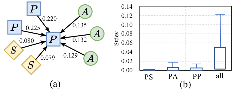
Figure 4: (a) An illustration of the observation that HGB tends to assign similar attention values within each relation for each target node. (b) The box plot of standard deviations of attention values for different relations in HGB.

	RGCN	HetGNN	HAN	MAGNN
Feature projection	$\textbf{h}_{v}^{r}=W^{\psi(r)}\textbf{x}_{v}$	$\textbf{h}^{\prime}_{v}={\rm Bi\raisebox{0.0pt}{-}LSTM}^{\phi(v)}(\textbf{x}_{v})$	$\textbf{h}^{\prime}_{v}=W^{\phi(v)}\textbf{x}_{v}$
Neighbor aggregation	$\textbf{z}_{v}^{r}=\frac{1}{|\mathcal{N}_{v}^{r}|}\sum_{u\in\mathcal{N}_{v}^{r}}\textbf{h}^{r}_{u}$	$\textbf{z}_{v}^{t}={\rm Bi\raisebox{0.0pt}{-}LSTM}(\{\textbf{h}^{\prime}_{u}:u\in\mathcal{N}_{v}^{t}\})$	$\gamma^{\mathcal{P}}_{v,u}=\sigma(\textbf{a}^{T}_{\mathcal{P}}\cdot[\textbf{h}^{\prime}_{v}||\textbf{h}^{\prime}_{u}])$	$\textbf{h}^{\prime}_{p(v,u)}={\rm Encoder}(p(v,u))$ $\gamma^{\mathcal{P}}_{v,u}=\sigma(\textbf{a}^{T}_{\mathcal{P}}\cdot[\textbf{h}^{\prime}_{v}||\textbf{h}^{\prime}_{p(v,u)}])$
			$\alpha^{\mathcal{P}}_{v,u}=\frac{\exp(\gamma^{\mathcal{P}}_{v,u})}{\sum_{k\in\mathcal{N}^{\mathcal{P}}_{v}}\exp(\gamma^{\mathcal{P}}_{v,k})},\,\,\textbf{z}^{\mathcal{P}}_{v}=\sigma(\sum_{k\in\mathcal{N}^{\mathcal{P}}_{v}}\alpha^{\mathcal{P}}_{v,k}\textbf{h}^{\prime}_{p(v,k)})$
Semantic fusion	$\textbf{h}_{v}=\sum_{r}\textbf{z}_{v}^{r}+W_{0}\textbf{x}_{v}$	$\alpha_{v}^{t}=\frac{\exp{({\rm LeakyReLU}(\textbf{a}^{T}[\textbf{z}_{v}^{t}||\textbf{h}^{\prime}_{v}]))}}{\sum_{k}\exp{({\rm LeakyReLU}(\textbf{a}^{T}[\textbf{z}_{v}^{k}||\textbf{h}^{\prime}_{v}]))}}$ $\textbf{h}_{v}=\alpha_{v}\textbf{h}^{\prime}_{v}+\sum_{t}\alpha_{v}^{t}\textbf{z}^{t}_{v}$	$w_{\mathcal{P}}=\frac{1}{||V^{\phi(v)}||}\sum_{k\in V^{\phi(v)}}\textbf{q}^{T}\cdot\tanh(\textbf{W}\textbf{z}_{k}^{\mathcal{P}}+\textbf{b})$ $\beta_{\mathcal{P}_{i}}=\frac{\exp(w_{P_{i}})}{\sum_{\mathcal{P}_{j}}\exp(w_{P_{j}})},\,\,\textbf{h}_{v}=\sum_{\mathcal{P}_{i}}\beta_{\mathcal{P}_{i}}\textbf{z}^{\mathcal{P}_{i}}_{v}$

Table 6: The unified framework of existing metapath-based HGNNs.

In our re-implemention experiments of HGB, we find that the attention values are mainly dominated by the edge-type embeddings. This is revealed from the observation that attention values within each relation are similar, while those among different relations ary significantly. Figure 4 (a) depicts this observation and Figure 4 (b) shows the statistics of standard deviations of attention values within each relation and among all relations for each target node on the ACM dataset.

This observation motivates us to investigate the necessity of neighbor attention within each relation and semantic attention among different relations in HGNNs.

Framework of existing metapath-based methods

For each layer of existing metapath-based methods, the calculation can be divided into three primary steps, feature projection, neighbor aggregation, and semantic fusion, as presented in Table 6. The feature projection step aims to map raw feature vectors of different types of nodes into the same data space, usually presented as one linear projection layer. Then the neighbor aggregation step aggregates feature vectors of neighbors for each semantic scope, e.g., for each relation (can be viewed as 1-hop metapath) in RGCN, for each node type in HetGNN, or for each metapath in HAN and MAGNN. Finally, the semantic aggregation step fuses those semantic vectors across all semantics and outputs the final embedding for each node.

After removing neighbor attention, since both the one-layer feature projection and neighbor aggregation contain no nonlinear functions, the order of the two steps can be exchanged. Further, as the neighbor aggregation step does not involve any trainable parameters, it can be put ahead in the pre-processing step, and its results are shared across all training epochs.

In later experiments, we find a multi-layer block for feature projection can further enhance the performance. Therefore, SeHGNN employs an MLP block rather than a single linear layer for each metapath in the feature projection step.

Experiment settings

The evaluation of SeHGNN involves four medium-scale datasets from HGB benchmark (Lv et al. 2021) and a large-scale dataset ogbn-mag from the OGB challenge (Hu et al. 2021). The statistics of these heterogeneous graphs are summarized in Table 7. For the medium-scale datasets, we follow the dataset configuration requirements of the HGB benchmark. Specifically, the target type nodes are split with 30% for local training and 70% for online test, where labels of test nodes are not made public and researchers have to submit their predictions to the website of HGB benchmark for online evaluation. For local training, we randomly split the 30% nodes into 24% for training for 6% for validation. We compare our results with the baseline scores reported in the HGB paper, and all scores are the average of 5 different local data partitions. For the ogbn-mag dataset, we follows the official data partition where papers published before 2018, in 2018, and since 2019 are nodes for training, validation, and test, respectively. We compare our results with the scores on the OGB leaderboard, and all scores are the average of 10 separate trainings.

Dataset	#Nodes	#Node types	#Edges	#Classes
DBLP	26,128	4	239,566	4
ACM	10,942	4	547,872	3
IMDB	21,420	4	86,642	5
Freebase	180,098	8	1,057,688	7
Ogbn-mag	1,939,743	4	21,111,007	349

Table 7: The statistics of datasets used in this paper.

	Feature propagation		Label Propagation
	Max Hop	#Metapaths	Max Hop	#Metapaths
DBLP	2	5	4	4
IMDB	4	25	4	12
ACM	4	41	3	9
Freebase	2	73	3	9
Ogbn-mag	2	10	2	5

Table 8: The maximum hops and numbers of metapaths for raw feature propagation and label propagation.

We adopt a simple metapath selection method where we preset the maximum hop and use all available metapaths no more than this maximum hop. We test different combinations of maximum hops for raw feature propagation and label propagation and the final choices are listed in Figure 8.

For all experiments, SeHGNN adopts a two-layer MLP for each metapath in the feature projection step, where the dimension of hidden vectors is 512. In the transformer-based fusion module, the dimension of query and key vectors are 1/4 of hidden vectors, the dimension of value vectors equals that of hidden vectors, and the number of heads is 1.

SeHGNN is optimized with Adam (Kingma and Ba 2015) during training. The learning rate is 0.0003 and the weight decay is 0.0001 for the Freebase dataset, and the learning rate is 0.001 and the weight decay is 0 for others.

Further analysis of time complexity

	Feature projection	Neighbor aggregation	Semantic fusion
HAN	$O((n{+}m)d^{2})$	$O(nke_{1}d{+}(n{+}m)kd)$	$O(nkd^{2})$
HGB	$O((n{+}m)ld^{2})$	$O(ne_{2}d{+}(n{+}m)ld)$

Table 9: Revised time complexity on HAN and HGB with consideration of nodes of all types.

The computation complexity of HAN and HGB methods is challenging to estimate as it encompasses various node types and the reuse of projected neighbor node features in the neighbor aggregation step. To make a straightforward comparison, Table 5 includes the complexity of linear projection for target type nodes in HAN and HGB but omits that of nodes of other types. As illustrated in Table 9, we add the computation complexity of nodes of other types assuming the number of these nodes involved in one training batch to be $m$. These additions include the linear projection in the feature projection step and the calculation of neighbor attentions in the neighbor aggregation step.

When training in full-batch mode, $n$ and $m$ represent the total number of target type nodes and other type nodes in the heterogeneous graph, respectively. If $n$ and $m$ are comparable, i.e., $O(n)=O(m)$, then results in Table 9 can be reduced to those in Table 5.

However, for mini-batch training, $m$ can be significantly larger than $n$ for each training batch. In the case of a small batch size $n$ and almost no reusable projected neighbor node features, $m$ increases exponentially with the metapath length or number of layers (i.e., $O(m)=O(nke_{1})$ for HAN and $O(m)=O(ne_{2})$ for HGB). In this scenario, the computation complexity results on HAN and HGB in Table 5 show a significant under-estimation.

In contrast, estimating the computation complexity of SeHGNN is much simpler. Because the neighbor aggregation is calculated in the pre-processing step, eliminating the involvement of nodes of other types in each training batch.

References

- Bansal et al. (2019) Bansal, T.; Juan, D.-C.; Ravi, S.; and McCallum, A. 2019. A2N: Attending to neighbors for knowledge graph inference. In Proceedings of the 57th annual meeting of the association for computational linguistics, 4387–4392.
- Dong et al. (2020) Dong, Y.; Hu, Z.; Wang, K.; Sun, Y.; and Tang, J. 2020. Heterogeneous Network Representation Learning. In IJCAI, volume 20, 4861–4867.
- Fan et al. (2019) Fan, S.; Zhu, J.; Han, X.; Shi, C.; Hu, L.; Ma, B.; and Li, Y. 2019. Metapath-guided heterogeneous graph neural network for intent recommendation. In Proceedings of the 25th ACM SIGKDD international conference on knowledge discovery & data mining, 2478–2486.
- Fu et al. (2020) Fu, X.; Zhang, J.; Meng, Z.; and King, I. 2020. Magnn: Metapath aggregated graph neural network for heterogeneous graph embedding. In Proceedings of The Web Conference 2020, 2331–2341.
- Hamilton, Ying, and Leskovec (2017) Hamilton, W.; Ying, Z.; and Leskovec, J. 2017. Inductive representation learning on large graphs. Advances in neural information processing systems, 30.
- Hong et al. (2020) Hong, H.; Guo, H.; Lin, Y.; Yang, X.; Li, Z.; and Ye, J. 2020. An attention-based graph neural network for heterogeneous structural learning. In Proceedings of the AAAI Conference on Artificial Intelligence, volume 34, 4132–4139.
- Hu et al. (2021) Hu, W.; Fey, M.; Ren, H.; Nakata, M.; Dong, Y.; and Leskovec, J. 2021. OGB-LSC: A Large-Scale Challenge for Machine Learning on Graphs. In Vanschoren, J.; and Yeung, S., eds., Proceedings of the Neural Information Processing Systems Track on Datasets and Benchmarks, volume 1.
- Hu et al. (2020a) Hu, W.; Fey, M.; Zitnik, M.; Dong, Y.; Ren, H.; Liu, B.; Catasta, M.; and Leskovec, J. 2020a. Open graph benchmark: Datasets for machine learning on graphs. Advances in neural information processing systems, 33: 22118–22133.
- Hu et al. (2020b) Hu, Z.; Dong, Y.; Wang, K.; and Sun, Y. 2020b. Heterogeneous graph transformer. In Proceedings of The Web Conference 2020, 2704–2710.
- Kingma and Ba (2015) Kingma, D. P.; and Ba, J. 2015. Adam: A Method for Stochastic Optimization. In Bengio, Y.; and LeCun, Y., eds., International Conference on Learning Representations, ICLR 2015.
- Kipf and Welling (2017) Kipf, T. N.; and Welling, M. 2017. Semi-Supervised Classification with Graph Convolutional Networks. In International Conference on Learning Representations, ICLR 2017.
- Li, Han, and Wu (2018) Li, Q.; Han, Z.; and Wu, X.-M. 2018. Deeper insights into graph convolutional networks for semi-supervised learning. In Thirty-Second AAAI conference on artificial intelligence.
- Lin et al. (2022) Lin, H.; Yan, M.; Ye, X.; Fan, D.; Pan, S.; Chen, W.; and Xie, Y. 2022. A Comprehensive Survey on Distributed Training of Graph Neural Networks. arXiv preprint arXiv:2211.05368.
- Liu et al. (2022a) Liu, X.; Yan, M.; Deng, L.; Li, G.; Ye, X.; and Fan, D. 2022a. Sampling Methods for Efficient Training of Graph Convolutional Networks: A Survey. IEEE/CAA Journal of Automatica Sinica, 9(2): 205–234.
- Liu et al. (2022b) Liu, X.; Yan, M.; Deng, L.; Li, G.; Ye, X.; Fan, D.; Pan, S.; and Xie, Y. 2022b. Survey on Graph Neural Network Acceleration: An Algorithmic Perspective. In Raedt, L. D., ed., Proceedings of the Thirty-First International Joint Conference on Artificial Intelligence, IJCAI-22, 5521–5529.
- Liu et al. (2018) Liu, Z.; Chen, C.; Yang, X.; Zhou, J.; Li, X.; and Song, L. 2018. Heterogeneous graph neural networks for malicious account detection. In Proceedings of the 27th ACM international conference on information and knowledge management, 2077–2085.
- Lv et al. (2021) Lv, Q.; Ding, M.; Liu, Q.; Chen, Y.; Feng, W.; He, S.; Zhou, C.; Jiang, J.; Dong, Y.; and Tang, J. 2021. Are we really making much progress? Revisiting, benchmarking and refining heterogeneous graph neural networks. In Proceedings of the 27th ACM SIGKDD Conference on Knowledge Discovery & Data Mining, 1150–1160.
- Niu et al. (2020) Niu, X.; Li, B.; Li, C.; Xiao, R.; Sun, H.; Deng, H.; and Chen, Z. 2020. A dual heterogeneous graph attention network to improve long-tail performance for shop search in e-commerce. In Proceedings of the 26th ACM SIGKDD International Conference on Knowledge Discovery & Data Mining, 3405–3415.
- Rossi et al. (2020) Rossi, E.; Frasca, F.; Chamberlain, B.; Eynard, D.; Bronstein, M.; and Monti, F. 2020. Sign: Scalable inception graph neural networks. arXiv preprint arXiv:2004.11198.
- Schlichtkrull et al. (2018) Schlichtkrull, M.; Kipf, T. N.; Bloem, P.; Berg, R. v. d.; Titov, I.; and Welling, M. 2018. Modeling relational data with graph convolutional networks. In European semantic web conference, 593–607. Springer.
- Shi et al. (2016) Shi, C.; Li, Y.; Zhang, J.; Sun, Y.; and Philip, S. Y. 2016. A survey of heterogeneous information network analysis. IEEE Transactions on Knowledge and Data Engineering, 29(1): 17–37.
- Shi et al. (2021) Shi, Y.; Huang, Z.; Feng, S.; Zhong, H.; Wang, W.; and Sun, Y. 2021. Masked Label Prediction: Unified Message Passing Model for Semi-Supervised Classification. In Zhou, Z.-H., ed., Proceedings of the Thirtieth International Joint Conference on Artificial Intelligence, IJCAI-21, 1548–1554.
- Sun, Gu, and Hu (2021) Sun, C.; Gu, H.; and Hu, J. 2021. Scalable and adaptive graph neural networks with self-label-enhanced training. arXiv preprint arXiv:2104.09376.
- Sun, Lin, and Zhu (2020) Sun, K.; Lin, Z.; and Zhu, Z. 2020. Multi-stage self-supervised learning for graph convolutional networks on graphs with few labeled nodes. In Proceedings of the AAAI Conference on Artificial Intelligence, volume 34, 5892–5899.
- Sun and Han (2012) Sun, Y.; and Han, J. 2012. Mining heterogeneous information networks: principles and methodologies. Synthesis Lectures on Data Mining and Knowledge Discovery, 3(2): 1–159.
- Sun et al. (2011) Sun, Y.; Han, J.; Yan, X.; Yu, P. S.; and Wu, T. 2011. Pathsim: Meta path-based top-k similarity search in heterogeneous information networks. Proceedings of the VLDB Endowment, 4(11): 992–1003.
- Trouillon et al. (2016) Trouillon, T.; Welbl, J.; Riedel, S.; Gaussier, É.; and Bouchard, G. 2016. Complex embeddings for simple link prediction. In International conference on machine learning, 2071–2080. PMLR.
- Vashishth et al. (2020) Vashishth, S.; Sanyal, S.; Nitin, V.; and Talukdar, P. 2020. Composition-based Multi-Relational Graph Convolutional Networks. In International Conference on Learning Representations.
- Vaswani et al. (2017) Vaswani, A.; Shazeer, N.; Parmar, N.; Uszkoreit, J.; Jones, L.; Gomez, A. N.; Kaiser, Ł.; and Polosukhin, I. 2017. Attention is all you need. Advances in neural information processing systems, 30.
- Veličković et al. (2018) Veličković, P.; Cucurull, G.; Casanova, A.; Romero, A.; Liò, P.; and Bengio, Y. 2018. Graph Attention Networks. International Conference on Learning Representations, ICLR 2018.
- Wang and Leskovec (2020) Wang, H.; and Leskovec, J. 2020. Unifying graph convolutional neural networks and label propagation. arXiv preprint arXiv:2002.06755.
- Wang et al. (2021a) Wang, S.; Wei, X.; Nogueira dos Santos, C. N.; Wang, Z.; Nallapati, R.; Arnold, A.; Xiang, B.; Yu, P. S.; and Cruz, I. F. 2021a. Mixed-curvature multi-relational graph neural network for knowledge graph completion. In Proceedings of the Web Conference 2021, 1761–1771.
- Wang et al. (2020) Wang, X.; Bo, D.; Shi, C.; Fan, S.; Ye, Y.; and Yu, P. S. 2020. A survey on heterogeneous graph embedding: methods, techniques, applications and sources. arXiv preprint arXiv:2011.14867.
- Wang et al. (2019) Wang, X.; Ji, H.; Shi, C.; Wang, B.; Ye, Y.; Cui, P.; and Yu, P. S. 2019. Heterogeneous graph attention network. In The world wide web conference, 2022–2032.
- Wang et al. (2021b) Wang, Y.; Jin, J.; Zhang, W.; Yu, Y.; Zhang, Z.; and Wipf, D. 2021b. Bag of tricks of semi-supervised classification with graph neural networks. arXiv preprint arXiv:2103.13355.
- Wu et al. (2019) Wu, F.; Souza, A.; Zhang, T.; Fifty, C.; Yu, T.; and Weinberger, K. 2019. Simplifying graph convolutional networks. In International conference on machine learning, 6861–6871. PMLR.
- Wu et al. (2020) Wu, Z.; Pan, S.; Chen, F.; Long, G.; Zhang, C.; and Philip, S. Y. 2020. A comprehensive survey on graph neural networks. IEEE transactions on neural networks and learning systems, 32(1): 4–24.
- Yan et al. (2022) Yan, M.; Zou, M.; Yang, X.; Li, W.; Ye, X.; Fan, D.; and Xie, Y. 2022. Characterizing and Understanding HGNNs on GPUs. IEEE Computer Architecture Letters, 21(2): 69–72.
- Yang et al. (2020) Yang, C.; Xiao, Y.; Zhang, Y.; Sun, Y.; and Han, J. 2020. Heterogeneous network representation learning: A unified framework with survey and benchmark. IEEE Transactions on Knowledge and Data Engineering.
- Yang et al. (2021) Yang, H.; Yan, X.; Dai, X.; Chen, Y.; and Cheng, J. 2021. Self-enhanced gnn: Improving graph neural networks using model outputs. In 2021 International Joint Conference on Neural Networks (IJCNN), 1–8. IEEE.
- Yu et al. (2020) Yu, L.; Shen, J.; Li, J.; and Lerer, A. 2020. Scalable graph neural networks for heterogeneous graphs. arXiv preprint arXiv:2011.09679.
- Zhang et al. (2019) Zhang, C.; Song, D.; Huang, C.; Swami, A.; and Chawla, N. V. 2019. Heterogeneous graph neural network. In Proceedings of the 25th ACM SIGKDD International Conference on Knowledge Discovery & Data Mining, 793–803.
- Zhang et al. (2022) Zhang, W.; Yin, Z.; Sheng, Z.; Li, Y.; Ouyang, W.; Li, X.; Tao, Y.; Yang, Z.; and Cui, B. 2022. Graph Attention Multi-Layer Perceptron. In Proceedings of the 28th ACM SIGKDD Conference on Knowledge Discovery and Data Mining, KDD ’22, 4560–4570. ISBN 9781450393850.
- Zheng et al. (2022) Zheng, X.; Liu, Y.; Pan, S.; Zhang, M.; Jin, D.; and Yu, P. S. 2022. Graph Neural Networks for Graphs with Heterophily: A Survey. arXiv preprint arXiv:2202.07082.
- Zhu et al. (2019) Zhu, S.; Zhou, C.; Pan, S.; Zhu, X.; and Wang, B. 2019. Relation structure-aware heterogeneous graph neural network. In 2019 IEEE international conference on data mining (ICDM), 1534–1539. IEEE.