Adaptive deep learning for nonlinear time series models

Abstract.

In this paper, we develop a general theory for adaptive nonparametric estimation of the mean function of a nonstationary and nonlinear time series model using deep neural networks (DNNs). We first consider two types of DNN estimators, non-penalized and sparse-penalized DNN estimators, and establish their generalization error bounds for general nonstationary time series. We then derive minimax lower bounds for estimating mean functions belonging to a wide class of nonlinear autoregressive (AR) models that include nonlinear generalized additive AR, single index, and threshold AR models. Building upon the results, we show that the sparse-penalized DNN estimator is adaptive and attains the minimax optimal rates up to a poly-logarithmic factor for many nonlinear AR models. Through numerical simulations, we demonstrate the usefulness of the DNN methods for estimating nonlinear AR models with intrinsic low-dimensional structures and discontinuous or rough mean functions, which is consistent with our theory.

1. Introduction

Motivated by the great success of deep neural networks (DNNs) in several applications such as pattern recognition and natural language processing, there has been an increasing interest in revealing the reason why DNNs work well from the statistical point of view. In the past few years, many researchers have contributed to understand theoretical advantages of DNN estimates for nonparametric regression models. See, for example, Bauer and Kohler (2019), Imaizumi and Fukumizu (2019), Schmidt-Hieber (2019, 2020), Suzuki (2019), Hayakawa and Suzuki (2020), Nakada and Imaizumi (2020), Kohler and Langer (2021), Suzuki and Nitanda (2021), Tsuji and Suzuki (2021), and references therein.

In contrast to the recent progress of DNNs, theoretical results on statistical properties of DNN methods for stochastic processes are scarce. As exceptional studies, we refer to Phandoidaen and Richter (2020), Kohler and Krzyzak (2023), Ogihara (2021), and Oga and Koike (2021). Phandoidaen and Richter (2020) investigates forecasting ability of feed-forward DNNs for stationary processes and derive bounds for an expected forecast error. Kohler and Krzyzak (2023) consider a time series prediction problem and investigate the convergence rate of a deep recurrent neural network estimate. Ogihara (2021) considers DNN estimation for the diffusion matrices and studies their estimation errors as misspecified parametric models. Oga and Koike (2021) investigate nonparametric drift estimation of a multivariate diffusion process. Notably, there seem no theoretical results on the statistical properties of feed-forward DNN estimators for nonparametric estimation of the mean functions of nonlinear and possibly nonstationary time series models.

The goal of this paper is to develop a general theory for adaptive nonparametric estimation of the mean function of a nonlinear time series using DNNs. The contributions of this paper are as follows.

First, we provide bounds of (i) generalization error (Lemma C.1) and (ii) expected empirical error (Lemma C.2) of general estimators of the mean function of a nonlinear and nonstationary $\beta$-mixing time series. We note that Lemma C.1 allows the $\beta$-mixing coefficients to decay both polynomially and exponentially fast and are of independent theoretical interest since they can be useful to investigate asymptotic properties of nonparametric estimators including DNNs. Building upon the results, we establish a generalization error bound of non-penalized DNN estimators (Theorem 3.1) with a $C$-Lipschitz activation function (e.g., rectified linear unit (ReLU), LeakyReLU, sigmoid, and softplus).

Second, we consider a sparse-penalized DNN estimator which is defined as a minimizer of an empirical risk with a sparse penalty and develop its asymptotic properties. In particular, we establish a generalization error bound of the sparse penalized DNN estimator (Theorem 3.2) with a $C$-Lipschitz activation function when the observations are $\beta$-mixing and can be nonstationary. While the result is shown under the condition that the $\beta$-mixing coefficients decay exponentially fast, it is straightforward to extend it to the case that the $\beta$-mixing coefficients decay polynomially fast. We note that our conditions on the penalty function cover several examples such as the clipped $L_{1}$ penalty (Zhang, 2010b), the SCAD penalty (Fan and Li, 2001), the minimax concave penalty (Zhang, 2010a), and the seamless $L_{0}$ penalty (Dicker et al., 2013), and the generalization error bound enables us to estimate mean functions of nonlinear time series models adaptively. Our work can be viewed as extensions of the results in Schmidt-Hieber (2020) and Ohn and Kim (2022) for independent observations to nonstationary time series. From the technical point of view, our analysis is related to the strategy in Schmidt-Hieber (2020). Due to the existence of temporal dependence, the extensions are nontrivial and we achieve this by developing a new strategy to obtain generalization error bounds for dependent data using a blocking technique for $\beta$-mixing processes and exponential inequalities for self-normalized martingale difference sequences. It shall be noted that our approach is also quite different from that of Ohn and Kim (2022) since their approach strongly depends on the independence of observations and our generalization error bounds of the sparse penalized DNN estimator improve the power of the logs in their bounds. More detailed differences are discussed in Section 3.3 and the supplementary material. Our approach to deriving generalization error bounds paves a way to new techniques for studying statistical properties of machine learning methods for more richer classes of models for dependent data including time series and spatial data.

Third, we establish that the sparse-penalized DNN estimators achieve minimax rates of convergence up to a poly-logarithmic factor over a wide class of nonlinear AR($d$) processes including generalized additive AR models and functional coefficient AR models introduced in Chen and Tsay (1993) that allow discontinuous mean functions. When the mean function belongs to a class of suitably smooth functions (e.g., Hölder space), one can use other nonparametric estimators for adaptively estimating the mean function (see Hoffmann (1999) for example). Similar assumptions on the smoothness of the mean functions have been made in most papers that investigate nonparametric estimation of the mean functions of nonlinear and stationary time series models (Robinson (1983), Tran (1993), Truong (1994), Masry (1996a, b), Hoffmann (1999), Fan and Yao (2008), Zhao and Wu (2008), Hansen (2008), Liu and Wu (2010)). Vogt (2012) and Zhang and Wu (2015) investigate nonparametric regression of locally stationary (i.e., nonstationary) models. The authors derive uniform convergence rates of kernel estimators of general smooth mean functions. Vogt (2012) also considers nonparametric estimation of additive mean functions. The generalization error bounds (Theorems 3.1 and 3.2) in this paper can be applied to nonstationary time series models with more general mean functions that include those considered in Vogt (2012) and Zhang and Wu (2015). However, the methods in those papers cannot be applied for estimating nonlinear time series models with possibly discontinuous mean functions. Our results show that the sparse-penalized DNN estimation is a unified method for adaptively estimating both smooth and discontinuous mean functions of time series regression models. Further, we shall note that the sparse-penalized DNN estimators attain the parametric rate of convergence up to a logarithmic factor when the mean functions belong to an $\ell^{0}$-bounded affine class that include (multi-regime) threshold AR processes (Theorems 4.3 and 4.4).

In addition to the theoretical results, we also conduct simulation studies to investigate the finite sample performance of the DNN estimators. We find that the DNN methods work well for the models with (i) intrinsic low-dimensional structures and (ii) discontinuous or rough mean functions. These results are consistent with our main results.

To summarize, this paper contributes to the literature on nonparametric estimation of nonlinear and nonstationary time series by establishing (i) the theoretical validity of non-penalized and sparse-penalized DNN estimators for the adaptive nonparametric estimation of mean functions of nonlinear time series models and (ii) show the optimality of the sparse-penalized DNN estimator for a wide class of nonlinear AR processes.

The rest of the paper is organized as follows. In Section 2, we introduce nonparametric regression models considered in this paper and demonstrate that they cover a range of nonlinear time series models. In Section 3, we provide generalization error bounds of (i) the non-penalized and (ii) the sparse-penalized DNN estimators. In Section 4, we present the minimax optimality of the sparse-penalized DNN estimators and show that the estimators achieve the minimax optimal convergence rate up to a logarithmic factor over (i) composition structured functions and (ii) $\ell^{0}$-bounded affine classes. In Section 5, we provide simulation results. Section 6 concludes and discusses possible extensions. Proofs for Section 3 are given in Appendix A. The supplementary material includes a discussion of our main results (Section B), auxiliary lemmas (Section C), proofs for Section 4 (Section D), and technical tools (Section E).

1.1. Notations

For any $a,b\in\mathbb{R}$, we write $a\vee b=\max\{a,b\}$ and $a\wedge b=\min\{a,b\}$. For $x\in\mathbb{R}$, $\lfloor x\rfloor$ denotes the largest integer $\leq x$. Given a function $f$ defined on a subset of $\mathbb{R}^{d}$ containing $[0,1]^{d}$, we denote by $f|_{[0,1]^{d}}$ the restriction of $f$ to $[0,1]^{d}$. When $f$ is real-valued, we write $\|f\|_{\infty}:=\sup_{x\in[0,1]^{d}}|f(x)|$ for the supremum on the compact set $[0,1]^{d}$. Also, let $\operatorname{supp}(f)$ denote the support of the function $f$. For a vector or matrix $W$, we write $|W|$ for the Frobenius norm (i.e. the Euclidean norm for a vector), $|W|_{\infty}$ for the maximum-entry norm and $|W|_{0}$ for the number of non-zero entries. For any positive sequences $a_{n},b_{n}$, we write $a_{n}\lesssim b_{n}$ if there is a positive constant $C>0$ independent of $n$ such that $a_{n}\leq Cb_{n}$ for all $n$, $a_{n}\asymp b_{n}$ if $a_{n}\lesssim b_{n}$ and $b_{n}\lesssim a_{n}$.

2. Settings

Let $(\Omega,\mathcal{G},\{\mathcal{G}_{t}\}_{t\geq 0},\operatorname{P})$ be a filtered probability space. Consider the following nonparametric time series regression model:

$$Y_{t} =m(X_{t})+\eta(X_{t})v_{t},\ t=1,\dots,T,$$ (2.1)

where $T\geq 3$, $(Y_{t},X_{t})\in\mathbb{R}\times\mathbb{R}^{d}$, and $\{X_{t},v_{t}\}_{t=1}^{T}$ is a sequence of random vectors adapted to the filtration $\{\mathcal{G}_{t}\}_{t=1}^{T}$. We assume $C_{\eta}:=\sup_{x\in[0,1]^{d}}|\eta(x)|<\infty$. In this paper we investigate nonparametric estimation of the mean function $m$ on the compact set $[0,1]^{d}$, that is, $f_{0}:=m\mathbf{1}_{[0,1]^{d}}$. The model (2.1) covers a range of nonlinear time series models.

Example 2.1 (Nonlinear AR($p$)-ARCH($q$) model).

Consider a nonlinear AR model:

$$Y_{t} =\widetilde{m}(Y_{t-1},\dots,Y_{t-p})+(\gamma_{0}+\gamma_{1}Y_{t-1}^{2}+\dots+\gamma_{q}Y_{t-q}^{2})^{1/2}v_{t},$$

where $\gamma_{0}>0$, $\gamma_{i}\geq 0$, $i=1,\dots,q$ with $1\leq p,q\leq d$. This example corresponds to the model (2.1) with $X_{t}=(Y_{t-1},\dots,Y_{t-d})^{\prime}$, $m(x_{1},\dots,x_{d})=\widetilde{m}(x_{1},\dots,m_{p})$ and $\eta(x_{1},\dots,x_{d})=(\gamma_{0}+\gamma_{1}x_{1}^{2}+\dots+\gamma_{q}x_{q}^{2})^{1/2}$.

Example 2.2 (Multivariate nonlinear time series).

Consider the case that we observe multivariate time series $\{\mathbf{Y}_{t}=(Y_{1,t},\dots,Y_{p,t})^{\prime}\}_{t=1}^{T}$ and $\{\mathbf{X}_{t}=(X_{1,t},\dots,X_{d,t})^{\prime}\}_{t=1}^{T}$ such that

$$Y_{j,t} =m_{j}(\mathbf{X}_{t})+\eta_{j}(\mathbf{X}_{t})v_{j,t},\ j=1,\dots,p.$$ (2.2)

The model (2.2) corresponds to (i) multivariate nonlinear AR model when $\mathbf{X}_{t}=(\mathbf{Y}^{\prime}_{t-1},\dots,\mathbf{Y}^{\prime}_{t-q})^{\prime}$ for some $q\geq 1$ and (ii) multivariate nonlinear time series regression with exogenous variables when $\eta_{j}(\cdot)=1$ and $\{\mathbf{X}_{t}\}_{t=1}^{T}$ is uncorrelated with $\{\mathbf{v}_{t}=(v_{1,t},\dots,v_{p,t})^{\prime}\}_{t=1}^{T}$. If one is interested in estimating the mean function $\mathbf{m}=(m_{1},\dots,m_{p})^{\prime}:\mathbb{R}^{d}\to\mathbb{R}^{p}$, then it is enough to estimate each component $m_{j}$. In this case, the problem of estimating $m_{j}$ is reduced to that of estimating the mean function $m$ of the model (2.1).

Example 2.3 (Time-varying nonlinear models).

Consider a nonlinear time-varying model:

$$Y_{t} =m\left({t\over T},Y_{t-1},\dots,Y_{t-p}\right)+\eta\left({t\over T},Y_{t-1},\dots,Y_{t-q}\right)v_{t},$$ (2.3)

where $1\leq p,q\leq d-1$. This example corresponds to the model (2.1) with $X_{t}=(t/T,Y_{t-1},\dots,Y_{t-d+1})^{\prime}$ as well as $m$ and $\eta$ regarded as functions on $\mathbb{R}^{d}$ in the canonical way. If the random variables $v_{t}$ are i.i.d., then the model (2.3) corresponds to that considered in Vogt (2012). Moreover, the model (2.3) covers, for instance, time-varying AR($p$)-ARCH($q$) models when $m(u,x_{1},\dots,x_{p})=m_{0}(u)+\sum_{j=1}^{p}m_{j}(u)x_{j}$ and $\eta(u,x_{1},\dots,x_{q})=(\eta_{0}(u)+\sum_{j=1}^{q}\eta_{j}(u)x_{j}^{2})^{1/2}$ with some functions $m_{j}:[0,1]\to\mathbb{R}$, $\eta_{j}:[0,1]\to[0,\infty)$. By the same approach as in Example 2.2, the model (2.1) can be applied to multivariate time-varying nonlinear models.

3. Main results

In this section, we provide generalization error bounds of (i) the non-penalized and (ii) the sparse-penalized DNN estimators. First, we define the $\beta$-mixing coefficients of the possibly nonstationary process $\{X_{t}\}_{t=1}^{T}$. Recall that the process $\{X_{t}\}_{t=1}^{T}$ is defined on a filtered probability space $(\Omega,\mathcal{G},\{\mathcal{G}_{t}\}_{t\geq 0},\operatorname{P})$. Let $\mathcal{A}$ and $\mathcal{B}$ be subfields of $\mathcal{G}$. Define $\beta(\mathcal{A},\mathcal{B})=\sup{1\over 2}\sum_{i=1}^{I}\sum_{j=1}^{J}|\operatorname{P}(A_{i}\cap B_{j})-\operatorname{P}(A_{i})\operatorname{P}(B_{j})|$ where the supremum is taken over all pairs of (finite) partitions $\{A_{1},\dots,A_{I}\}$ and $\{B_{1},\dots,B_{J}\}$ of $\Omega$ such that $A_{i}\in\mathcal{A}$ and $B_{j}\in\mathcal{B}$. The $\beta$-mixing coefficients of the process $\{X_{t}\}_{t=1}^{T}$ is defined as $\beta_{X}(t):=\beta_{X,T}(t)=\sup_{1\leq r\leq T-t}\beta(\sigma(X_{s}:1\leq s\leq r),\sigma(X_{s}:r+t\leq s\leq T))$, where $\sigma(Z)$ is the $\sigma$-field generated by $Z$ (cf. Vogt (2012)). We assume the following conditions.

Assumption 3.1.

• The random variables $v_{t}$ are conditionally centered and sub-Gaussian, that is, $\mathrm{E}[v_{t}\mid\mathcal{G}_{t-1}]=0$ and $\mathrm{E}[\exp(v_{t}^{2}/K_{t}^{2})|\mathcal{G}_{t-1}]\leq 2$ for some constant $K_{t}>0$. Moreover, $\mathrm{E}[v_{t}^{2}|\mathcal{G}_{t-1}]=1$. Define $K=\max_{1\leq t\leq T}K_{t}$.

• The process $X=\{X_{t}\}_{t=1}^{T}$ is exponentially $\beta$-mixing, i.e. the $\beta$-mixing coefficient $\beta_{X}(t)$ of $X$ satisfies $\beta_{X}(t)\leq C_{1,\beta}\exp(-C_{2,\beta}t)$ with some positive constants $C_{1,\beta}$ and $C_{2,\beta}$ for all $t\geq 1$.

• The process $X$ is predictable, that is, $X_{t}$ is measurable with respect to $\mathcal{G}_{t-1}$.

Condition (i) is used to apply exponential inequalities for self-normalized processes presented in de la Peña et al. (2004). Since $\mathrm{E}[\mathrm{E}[\exp(v_{t}^{2}/K_{t}^{2})|\mathcal{G}_{t-1}]]=\mathrm{E}[\exp(v_{t}^{2}/K_{t}^{2})]$, Condition (i) also implies that each $v_{t}$ is sub-Gaussian. Condition (ii) is satisfied for a wide class of nonlinear time series. Note that the process $X=\{X_{t}\}_{t=1}^{T}$ can be nonstationary. When $X_{t}=(Y_{t-1},\dots,Y_{t-d})^{\prime}$, Chen and Chen (2000) provide a set of sufficient conditions for the process $X$ to be strictly stationary and exponentially $\beta$-mixing (Theorem 1 in Chen and Chen (2000)):

• $\{v_{t}\}$ is a sequence of i.i.d. random variables and has an everywhere positive and continuous density function, $E[v_{t}]=0$, and $v_{t}$ is independent of $X_{t-s}$ for all $s\geq 1$.

• The function $m$ is bounded on every bounded set, that is, for every $\Gamma\geq 0$, $\sup_{|x|\leq\Gamma}|m(x)|<\infty$.

• The function $\eta$ satisfies, for every $\Gamma\geq 0$, $0<\eta_{1}\leq\inf_{|x|\leq\Gamma}\eta(x)\leq\sup_{|x|\leq\Gamma}\eta(x)<\infty$, where $\eta_{1}$ is a constant.

• There exist constants $c_{m,i}\geq 0$, $c_{\eta,i}\geq 0$ ($i=0,\dots,d$) and $M>0$ such that $|m(x)|\leq c_{m,0}+\sum_{i=1}^{d}c_{m,i}|x_{i}|$ and $\eta(x)\leq c_{\eta,0}+\sum_{i=1}^{d}c_{\eta,i}|x_{i}|$ for $|x|\geq M$, and $\sum_{i=1}^{d}(c_{m,i}+c_{\eta,i}E[|v_{1}|])<1$.

We also refer to Tjøstheim (1990), Bhattacharya and Lee (1995), Lu and Jiang (2001), Cline and Pu (2004) and Vogt (2012) for other sufficient conditions for the process $X$ being strictly or locally stationary and exponentially $\beta$-mixing.

Remark 3.1.

Although the (exponential) $\beta$-mixing condition does not directly imply any kind of stationarity (as far as we know), for Markov processes it is implied by asymptotic stationarity (cf. Proposition 3 of Liebscher (2005)), and this sufficient condition is practically used to check the $\beta$-mixing condition. To our knowledge, locally stationary processes are the only known (non-artificial) examples satisfying the $\beta$-mixing condition without asymptotic stationarity. In particular, this condition seems to exclude explosive/unit-root cases, although we do not know any formal result in this direction.

3.1. Deep neural networks

To estimate the mean function $m$ of the model (2.1), we fit a deep neural network (DNN) with a nonlinear activation function $\sigma:\mathbb{R}\to\mathbb{R}$. The network architecture $(L,\mathbf{p})$ consists of a positive integer $L$ called the number of hidden layers or depth and a width vector $\mathbf{p}=(p_{0},\dots,p_{L+1})\in\mathbb{N}^{L+2}$. A DNN with network architecture $(L,\mathbf{p})$ is then any function of the form

$$f:\mathbb{R}^{p_{0}}\to\mathbb{R}^{p_{L+1}},\ x\mapsto f(x)=A_{L+1}\circ\sigma_{L}\circ A_{L}\circ\sigma_{L-1}\circ\dots\circ\sigma_{1}\circ A_{1}(x),$$ (3.1)

where $A_{\ell}:\mathbb{R}^{p_{\ell-1}}\to\mathbb{R}^{p_{\ell}}$ is an affine linear map defined by $A_{\ell}(x):=W_{\ell}x+\mathbf{b}_{\ell}$ for given $p_{\ell-1}\times p_{\ell}$ weight matrix $W_{\ell}$ and a shift vector $\mathbf{b}_{\ell}\in\mathbb{R}^{p_{\ell}}$, and $\sigma_{\ell}:\mathbb{R}^{p_{\ell}}\to\mathbb{R}^{p_{\ell}}$ is an element-wise nonlinear activation map defined as $\sigma_{\ell}(z):=(\sigma(z_{1}),\dots,\sigma(z_{p_{\ell}}))^{\prime}$. We assume that the activation function $\sigma$ is $C$-Lipschitz for some $C>0$, that is, there exists $C>0$ such that $|\sigma(x_{1})-\sigma(x_{2})|\leq C|x_{1}-x_{2}|$ for any $x_{1},x_{2}\in\mathbb{R}$. Examples of $C$-Lipschitz activation functions include the rectified linear unit (ReLU) activation function $x\mapsto\max\{x,0\}$ and the sigmoid activation function $x\mapsto 1/(1+e^{-x})$. For a neural network of the form (3.1), we define $\theta(f):=(\text{vec}(W_{1})^{\prime},\mathbf{b}^{\prime}_{1},\dots,\text{vec}(W_{L+1})^{\prime},\mathbf{b}^{\prime}_{L+1})^{\prime}$ where $\text{vec}(W)$ transforms the matrix $W$ into the corresponding vector by concatenating the column vectors.

We let $\mathcal{F}_{\sigma,p_{0},p_{L+1}}$ be the class of DNNs which take $p_{0}$-dimensional input to produce $p_{L+1}$-dimensional output and use the activation function $\sigma:\mathbb{R}\to\mathbb{R}$. Since we are interested in real-valued function on $\mathbb{R}^{d}$, we always assume that $p_{0}=d$ and $p_{L+1}=1$ in the following.

For a given DNN $f$, we let $\text{depth}(f)$ denote the depth and $\text{width}(f)$ denote the width of $f$ (i.e. $\text{width}(f)=\max_{1\leq\ell\leq L}p_{\ell}$). For positive constants $L,N,B$, and $F$, we set $\mathcal{F}_{\sigma}(L,N,B):=\{f\in\mathcal{F}_{\sigma,d,1}:\text{depth}(f)\leq L,\text{width}(f)\leq N,|\theta(f)|_{\infty}\leq B\}$ and

$$\mathcal{F}_{\sigma}(L,N,B,F):=\left\{f\mathbf{1}_{[0,1]^{d}}:f\in\mathcal{F}_{\sigma}(L,N,B),\|f\|_{\infty}\leq F\right\}.$$ (3.2)

Moreover, we define a class of sparsity constrained DNNs with sparsity level $S>0$ by

$$\mathcal{F}_{\sigma}(L,N,B,F,S) :=\left\{f\in\mathcal{F}_{\sigma}(L,N,B,F):|\theta(f)|_{0}\leq S\right\}.$$ (3.3)

3.2. Non-penalized DNN estimator

Let $\widehat{f}_{T}$ be an estimator which is a real-valued random function on $\mathbb{R}^{p}$ such that the map $(\omega,x)\mapsto\widehat{f}_{T}(\omega,x)$ is measurable with respect to the product of the $\sigma$-field generated by $\{Y_{t},X_{t}\}_{t=1}^{T}$ and the Borel $\sigma$-field of $\mathbb{R}^{d}$. In this section, we provide finite sample properties of a DNN estimator $\widehat{f}_{T}\in\mathcal{F}_{\sigma}(L,N,B,F,S)$ of $f_{0}$.

In particular, we provide bounds for the generalization error

$$R(\widehat{f}_{T},f_{0})=\mathrm{E}\left[{1\over T}\sum_{t=1}^{T}(\widehat{f}_{T}(X_{t}^{\ast})-f_{0}(X_{t}^{\ast}))^{2}\right],$$

where $\{X_{t}^{\ast}\}_{t=1}^{T}$ is an independent copy of $X$.

Remark 3.2.

When $\{X_{t}\}_{t\geq 1}$ has the common marginal distribution $\Pi$, i.e. $X_{t}\sim\Pi$ for all $t\geq 1$, we can rewrite $R(\widehat{f}_{T},f_{0})$ as $R(\widehat{f}_{T},f_{0})=\operatorname{E}[\int|\widehat{f}_{T}(x)-f_{0}(x)|^{2}\Pi(dx)]$, so it can be interpreted as the $L^{2}$-risk of the estimator $\widehat{f}_{T}$ with respect to $\Pi$. In this case, we can also relate it to the so-called path-dependent generalization error using the $\beta$-mixing coefficient of $\{X_{t},Y_{t}\}_{t\geq 1}$ as follows. First, the path-dependent generalization error is introduced in Kuznetsov and Mohri (2017) and defined as $\widetilde{R}_{s}(\widehat{f}_{T},f_{0}):=\operatorname{E}[(\widehat{f}_{T}(X_{T+s})-f_{0}(X_{T+s}))^{2}\mid\{Y_{t},X_{t}\}_{1\leq t\leq T}]$, where $s\geq 1$ is a fixed integer. This quantity can be interpreted as an $s$-ahead forecast error of $\widehat{f}_{T}$ given observation data. Now, by Lemma E.1, we can construct a random vector $X_{T+s}^{*}$ in $\mathbb{R}^{d}$ independent of $\{Y_{t},X_{t}\}_{t=1}^{T}$ such that $X_{T+s}^{*}\overset{d}{=}X_{T+s}(\sim\Pi)$ and $P(X_{T+s}^{*}\neq X_{T+s})=\beta_{Z}(s)$, where $\beta_{Z}$ is the $\beta$-mixing coefficient of the process $Z_{t}=(X_{t},Y_{t})$, $t\geq 1$. Then we have

$$\widetilde{R}_{s}(\widehat{f}_{T},f_{0}) \leq\operatorname{E}\left[\left(\widehat{f}_{T}(X^{*}_{T+s})-f_{0}(X^{*}_{T+s})\right)^{2}\mid\{Y_{t},X_{t}\}_{t=1}^{T}\right]+4F^{2}\beta_{Z}(s)$$

$$=\int_{\mathbb{R}^{d}}|\widehat{f}_{T}(x)-f_{0}(x)|^{2}\Pi(dx)+4F^{2}\beta_{Z}(s),$$

provided that $\|\widehat{f}_{T}\|_{\infty}\vee\|f_{0}\|_{\infty}\leq F$ for some constant $F$. Hence $\operatorname{E}[\widetilde{R}_{s}(\widehat{f}_{T},f_{0})]\leq R(\widehat{f}_{T},f_{0})+4F^{2}\beta_{Z}(s)$. In particular, if the process $Z_{t}$ is $\beta$-mixing in the sense that $\beta_{Z}(s)\to 0$ as $s\to\infty$, then a bound for $R(\widehat{f}_{T},f_{0})$ gives sufficiently far ahead forecast error bounds.

Let $\mathcal{F}$ be a pointwise measurable class of real-valued functions on $\mathbb{R}^{d}$ (cf. Example 2.3.4 in van der Vaart and Wellner (1996)). Define $\Psi_{T}^{\mathcal{F}}(\widehat{f}_{T}):=\mathrm{E}\left[Q_{T}(\widehat{f}_{T})-\inf_{\bar{f}\in\mathcal{F}}Q_{T}(\bar{f})\right]$ where $Q_{T}(f)$ is the empirical risk of $f$ defined by $Q_{T}(f):={1\over T}\sum_{t=1}^{T}(Y_{t}-f(X_{t}))^{2}$. The function $\Psi_{T}^{\mathcal{F}}(\widehat{f}_{T})$ measures a gap between $\widehat{f}_{T}$ and an exact minimizer of $Q_{T}(f)$ subject to $f\in\mathcal{F}$. Define

$$\widehat{f}_{T,np}\in\mathop{\rm arg~{}min}\limits_{f\in\mathcal{F}_{\sigma}(L,N,B,F,S)}Q_{T}(f)$$

and we call $\widehat{f}_{T,np}$ as the non-penalized DNN estimator.

The next result gives a generalization error bound of $\widehat{f}_{T,np}$.

Theorem 3.1.

Suppose that Assumption 3.1 is satisfied. Consider the nonparametric time series regression model (2.1) with unknown regression function $m$ satisfying $\|f_{0}\|_{\infty}\leq F$ where $f_{0}=m\mathbf{1}_{[0,1]^{d}}$ for some $F\geq 1$. Let $\widehat{f}_{T}$ be any estimator taking values in the class $\mathcal{F}=\mathcal{F}_{\sigma}(L,N,B,F,S)$ with $B\geq 1$. Then for any $\rho>1$, there exists a constant $C_{\rho}$, only depending on $(C_{\eta},C_{1,\beta},C_{2,\beta},K,\rho)$, such that

$$R(\widehat{f}_{T},f_{0}) \leq\rho\left(\Psi_{T}^{\mathcal{F}}(\widehat{f}_{T})+\inf_{f\in\mathcal{F}}R(f,f_{0})\right)+C_{\rho}F^{2}{S(L+1)\log\left((L+1)(N+1)BT\right)(\log T)\over T}.$$

Theorem 3.1 is an extension of Theorem 2 in Schmidt-Hieber (2020) to possibly nonstationary $\beta$-mixing sequence and the process $\{v_{t}\}$ can be non Gaussian and dependent. The result follows from Lemmas C.1 and C.2 in the supplementary material. Note that these Lemmas are of independent interest since they are general results so that the estimator $\widehat{f}_{T}$ do not need to take values in $\mathcal{F}_{\sigma}(L,N,B,F,S)$. Hence the results would be useful to investigate generalization error bounds of other nonparametric estimators.

Let $f_{0}=m\mathbf{1}_{[0,1]^{d}}$ belong to composition structured functions $\mathcal{F}_{0}=\mathcal{G}\big{(}q,\mathbf{d},\mathbf{t},\bm{\beta},A\big{)}$ for example (see Section 4.1 for the definition). By choosing $\sigma(x)=\max\{x,0\}$ and the parameters of $\mathcal{F}_{\sigma}(L_{T},N_{T},B_{T},F,S_{T})$ as $L_{T}\asymp\log T$, $N_{T}\asymp T$, $B_{T}\geq 1$, $F>\|f_{0}\|_{\infty}$, and $S_{T}\asymp T^{\kappa/(\kappa+1)}\log T$ with $\kappa$ depending on $\mathbf{t}$ and $\bm{\beta}$, one can show that the non-penalized DNN estimator achieves the minimax convergence rate over $\mathcal{F}_{0}$ up to a logarithmic factor. However, the sparsity level $S_{T}$ depends on the characteristics $\mathbf{t}$ and $\bm{\beta}$ of $f_{0}$. Therefore, the non-penalized DNN estimator is not adaptive since we do not know the characteristics in practice. In the next subsection, we provide a generalization error bound of sparse-penalized DNN estimators which plays an important role to show that the sparse-penalized DNN estimators can estimate $f_{0}$ adaptively.

Remark 3.3 (Generalization error bound under $\beta$-mixing coefficients with polynomial decay).

We can also give a generalization error bound of the non-penalized DNN estimator $\widehat{f}_{T,np}$ under $\beta$-mixing coefficients with polynomial decay. Instead of Assuption 3.1 (ii), assume that $\beta_{X}(t)\leq C_{\beta}t^{-\alpha}$ for some $\alpha>0$. Then under the same assumptions in Theorem 3.1, we have

$$R(\widehat{f}_{T},f_{0}) \leq\rho\left(\Psi^{\mathcal{F}}(\widehat{f}_{T})+\inf_{f\in\mathcal{F}}R(f,f_{0})\right)+\overline{C}F^{2}\left({(\log T)(\log\mathcal{N}_{T})\over T}+\left({\log\mathcal{N}_{T}\over T}\right)^{{\alpha\over\alpha+1}}\right),$$ (3.4)

where $\mathcal{N}_{T}$ depends on the $T^{-1}$-covering number of $\mathcal{F}_{\sigma}(L,N,B,F,S)$ with respect to $\|\cdot\|_{\infty}$ and we can see that $\log\mathcal{N}_{T}\leq c_{1}S(L+1)\log\left((L+1)(N+1)BT\right)$ (see Appendix A and Section E of the supplementary material for the detailed definition the covering number and the bound of $\log\mathcal{N}_{T}$), respectively. Here, $c_{1}$ is a universal constant and $\overline{C}$ is a constant depending only on $(C_{\eta},C_{\beta},K,\rho)$. A similar generalization error bound can be derived for the sparse-penalized DNN, which is defined in the next subsection (see Remarks A.1 and A.2 in Appendix A for details). We speculate the bound (3.4) would be suboptimal (at least) when $\{X_{t}\}_{t=1}^{T}$ and $\{v_{t}\}_{t=1}^{T}$ are independent. On this point, we refer to Kulik and Lorek (2011) that investigates the convergence rate of the Nadaraya–Watson estimator for nonparametric time series regression models with serially correlated covariates and errors. See Section B of the supplementary material for a more detailed discussion on this point.

3.3. Sparse-penalized DNN estimator

Define $\bar{Q}_{T}(f)$ as a penalized version of the empirical risk $\bar{Q}_{T}(f):={1\over T}\sum_{t=1}^{T}(Y_{t}-f(X_{t}))^{2}+J_{T}(f)$ where $J_{T}(f)$ is the a sparse penalty of the form $J_{T}(f)=\sum_{j=1}^{p}\pi_{\lambda_{T},\tau_{T}}(\theta_{j}(f))$ with a function $\pi_{\lambda_{T},\tau_{T}}:\mathbb{R}\to[0,\infty)$ having two tuning parameters $\lambda_{T}>0$ and $\tau_{T}>0$. Here, $p$ is the length of the vector $\theta(f)$ and $\theta_{j}(f)$ denotes the $j$-th component of $\theta(f)$. We assume that $\pi_{\lambda_{T},\tau_{T}}$ satisfies the following conditions:

1. $\pi_{\lambda_{T},\tau_{T}}(0)=0$ and $\pi_{\lambda_{T},\tau_{T}}(\theta)$ is non-decreasing in $|\theta|$.

2. $\pi_{\lambda_{T},\tau_{T}}(\theta)=\lambda_{T}$ if $|\theta|>\tau_{T}$.

A prominent example is the clipped $L_{1}$ penalty of Zhang (2010b) which is given by

$$\pi_{\lambda_{T},\tau_{T}}(\theta)=\lambda_{T}\left({|\theta|\over\tau_{T}}\wedge 1\right).$$ (3.5)

This choice is used in Ohn and Kim (2022). Other possible choices are the SCAD penalty (Fan and Li, 2001), the minimax concave penalty (Zhang, 2010a) and the seamless $L_{0}$ penalty (Dicker et al., 2013). In this section, we provide finite sample properties of the sparse-penalized DNN estimator defined as

$$\widehat{f}_{T,sp}\in\mathop{\rm arg~{}min}\limits_{f\in\mathcal{F}_{\sigma}(L,N,B,F)}\bar{Q}_{T}(f).$$

Further, for any estimator $\widehat{f}_{T}\in\mathcal{F}=\mathcal{F}_{\sigma}(L,N,B,F)$ of $f_{0}$, we define
$\bar{\Psi}_{T}^{\mathcal{F}}(\widehat{f}_{T}):=\mathrm{E}\left[\bar{Q}_{T}(\widehat{f}_{T})-\inf_{\bar{f}\in\mathcal{F}}\bar{Q}_{T}(\bar{f})\right]$.

The next result provides a generalization error bound of the sparse-penalized DNN estimator.

Theorem 3.2.

Suppose that Assumption 3.1 is satisfied. Consider the nonparametric time series regression model (2.1) with unknown regression function $m$ satisfying $\|f_{0}\|_{\infty}\leq F$ where $f_{0}=m\mathbf{1}_{[0,1]^{d}}$ for some $F\geq 1$. Let $\widehat{f}_{T}$ be any estimator taking values in the class $\mathcal{F}=\mathcal{F}_{\sigma}(L_{T},N_{T},B_{T},F)$ where $L_{T},N_{T}$, and $B_{T}$ are positive values such that $L_{T}\leq C_{L}\log^{\nu_{0}}T$, $N_{T}\leq C_{N}T^{\nu_{1}}$, $1\leq B_{T}\leq C_{B}T^{\nu_{2}}$ for some positive constants $C_{L},C_{N},C_{B},\nu_{0},\nu_{1}$, and $\nu_{2}$. Moreover, we assume that the tuning parameters $\lambda_{T}$ and $\tau_{T}$ of the sparse penalty function $J_{T}(f)$ satisfy $\lambda_{T}=(F^{2}\iota_{\lambda}(T)\log^{2+\nu_{0}}T)/T$ with a strictly increasing function $\iota_{\lambda}(x)$ such that $\iota_{\lambda}(x)/\log x\to\infty$ as $x\to\infty$ and $\tau_{T}(L_{T}+1)((N_{T}+1)B_{T})^{L_{T}+1}\leq C_{\tau}T^{-1}$ with some positive constant $C_{\tau}$ for any $T$. Then,

$$R(\widehat{f}_{T},f_{0}) \leq 6\left(\bar{\Psi}_{T}^{\mathcal{F}}(\widehat{f}_{T})+\inf_{f\in\mathcal{F}}\left(R(f,f_{0})+J_{T}(f)\right)\right)+CF^{2}\left({1+\log T\over T}\right),$$

where $C$ is a positive constant only depending on $(C_{\eta},C_{1,\beta},C_{2,\beta},C_{L},C_{N},C_{B},C_{\tau},\nu_{0},\nu_{1},\nu_{2},K,\iota_{\lambda})$.

Theorem 3.2 is an extension of Theorem 1 in Ohn and Kim (2022), which considers i.i.d. observations. Here we explain some differences between their result and ours. First, our conditions on the penalty function cover the clipped $L_{1}$ penalty, which is considered in Ohn and Kim (2022), as a special case. Second, Theorem 3.2 can be applied to nonstationary time series since we only assume the process $X$ to be $\beta$-mixing. Third, our approach to proving Theorem 3.2 is different from that of Ohn and Kim (2022). Their proofs heavily depend on the theory for i.i.d. data in Györfi et al. (2002) so extending their approach to our framework seems to require substantial work. In contrast, our approach is based on other technical tools such as the blocking technique of $\beta$-mixing processes in Rio (2013) and exponential inequalities for self-normalized martingale difference sequences. In particular, considering continuous time embedding of a martingale difference sequence and applying the results on (super-) martingales in Barlow et al. (1986), we can allow the process $\{v_{t}\}_{t=1}^{T}$ to be conditionally centered and circumvent additional conditions on its distribution such as conditional Gaussianity or symmetry (see also Lemma E.2 and the proof of Lemma E.3 in the supplementary material). As a result, our result improves the power of logs in their generalization error bound. Fourth, (a) the upper bound of the depth of the sparse penalized DNN estimator $L$ can grow by a power of $\log T$ and (b) we take the tuning parameter $\lambda_{T}$ to depend on $F^{2}$. Particularly, (a) enables us to estimate $f_{0}$ adaptively when $f_{0}$ belongs to an $\ell^{0}$-bounded affine class as well as composition structured functions (see Sections 4.1 and 4.2 for details) and (b) enables $\widehat{f}_{T,sp}$ to be adaptive with respect to $\|f\|_{\infty}\leq F$. See also the comments on Proposition 4.1 on the improvement of the upper bound.

4. Minimax optimality in nonlinear AR models

In this section, we show the minimax optimality of the sparse-penalized DNN estimator $\widehat{f}_{T,sp}$. In particular, we show that $\widehat{f}_{T,sp}$ achieves the minimax convergence rate over (i) composition structured functions and (ii) $\ell^{0}$-bounded affine class. We note that these classes of functions include many nonlinear AR models such as (generalized) additive AR models, single-index models, (multi-regime) threshold AR models, and exponential AR models.

We consider the observation $\{Y_{t}\}_{t=1}^{T}$ generated by the following nonlinear AR($d$) model:

$$\left\{\begin{array}[]{l}Y_{t}=m(Y_{t-1},\dots,Y_{t-d})+v_{t},\qquad t=1,\dots,T,\\ v_{t}\overset{i.i.d.}{\sim}N(0,1),\qquad(Y_{0},Y_{-1},\dots,Y_{-d+1})^{\prime}\sim\nu.\end{array}\right.$$ (4.1)

Here, $\nu$ is a (fixed) probability measure on $\mathbb{R}^{d}$ such that $\int_{\mathbb{R}^{d}}|x|\nu(dx)<\infty$, and $m:\mathbb{R}^{d}\to\mathbb{R}$ is an unknown function to be estimated.

Remark 4.1.

Note that the process $\{Y_{t}\}_{t=1}^{T}$ is possibly non-stationary because the initial distribution $\nu$ is not necessarily the stationary distribution. However, below we impose conditions to ensure ergodicity of the process, so we require the model to be asymptotically stationary in this sense. This is necessary because we need an error bound uniformly valid over a class of mean functions to establish (near) minimax optimality. A major difficulty to obtain such a bound is establishing a uniform upper bound for $\beta$-mixing coefficients because it is unclear how most available bounds depend on model parameters. For this purpose we prove Lemma 4.1 using the technique developed in Hairer and Mattingly (2011). This is the place where we need assumptions to ensure ergodicity. By contrast, the setup in the previous sections allows for some asymptotically non-stationary models like locally stationary processes (cf. Example 2.3). We conjecture that a uniform $\beta$-mixing bound could be established for locally stationary processes under appropriate uniform versions of assumptions in (Vogt, 2012, Theorem 3.4), but this requires us to carefully examine the entire proof of this result. This is beyond the scope of the paper and we leave it to future research.

Let $\mathbf{c}=(c_{0},c_{1},\dots,c_{d})\in(0,\infty)^{d+1}$ satisfy $\sum_{i=1}^{d}c_{i}<1$. We denote by $\mathcal{M}_{0}(\mathbf{c})$ the set of measurable functions $m:\mathbb{R}^{d}\to\mathbb{R}$ satisfying $|m(x)|\leq c_{0}+\sum_{i=1}^{d}c_{i}|x_{i}|$ for all $x\in\mathbb{R}^{d}$. The following lemma shows that the process $Y=\{Y_{t}\}_{t=1}^{T}$ is exponentially $\beta$-mixing “uniformly” over $m\in\mathcal{M}_{0}(\mathbf{c})$.

Lemma 4.1.

Consider the nonlinear AR($d$) model (4.1) with $m\in\mathcal{M}_{0}(\mathbf{c})$. Let $\beta_{Y}(t)$ be the $\beta$-mixing coefficient of $Y$. There are positive constants $C_{\beta}$ and $C_{\beta}^{\prime}$ depending only on $\mathbf{c},d$ and $\nu$ such that

$$\beta_{Y}(t)\leq C^{\prime}_{\beta}e^{-C_{\beta}t}\qquad\text{for all }t\geq 1.$$ (4.2)

The next result gives a generalization error bound of DNN estimators for a family of functions that can be approximated with a certain degree of accuracy by DNNs.

Proposition 4.1.

Consider the nonlinear AR($d$) model (4.1) with $m\in\mathcal{M}_{0}(\mathbf{c})$. Let $F$, $\widehat{f}_{T}$, $\mathcal{F}$, $L_{T}$, $N_{T}$, $B_{T}$, $\lambda_{T}$ and $\tau_{T}$ as in Theorem 3.2. Suppose that there are constants $\kappa,r\geq 0$, $C_{0}>0$ and $C_{S}>0$ such that $\inf_{f\in\mathcal{F}_{\sigma}(L_{T},N_{T},B_{T},F,S_{T})}\|f-f_{0}\|_{L^{2}([0,1]^{d})}^{2}\leq C_{0}T^{-1/(\kappa+1)}$ with $S_{T}:=C_{S}T^{\kappa/(\kappa+1)}\log^{r}T$. Then,

$$R(\widehat{f}_{T},f_{0})\leq 6\bar{\Psi}_{T}^{\mathcal{F}}(\widehat{f}_{T})+C^{\prime}F^{2}\frac{\iota_{\lambda}(T)\log^{2+\nu_{0}+r}T}{T^{1/(\kappa+1)}},$$

where $C^{\prime}$ is a positive constant only depending on $(\!\mathbf{c},d,\nu,C_{L},C_{N},C_{B},C_{\tau},\nu_{0},\nu_{1},\nu_{2},K,\iota_{\lambda},\kappa,r,C_{0},C_{S}\!)$.

If $\widehat{f}_{T}=\widehat{f}_{T,sp}$, then the generalization error bound in Proposition 4.1 is reduced to $R(\widehat{f}_{T},f_{0})\leq C^{\prime}F^{2}\iota_{\lambda}(T)(\log^{2+\nu_{0}+r}T)T^{-1/(\kappa+1)}$. When $\nu_{0}=1$ and $\iota_{\lambda}(T)=\log^{\nu_{3}}T$ with $\nu_{3}\in(1,2)$, one can see that our result improves the power of logs in the generalization error bound in Theorem 2 in Ohn and Kim (2022). Moreover, our result allows the generalization error bound to depend explicitly on $F$. Combining this with the results in the following sections implies that the sparse-penalized DNN estimator can be adaptive concerning the upper bound of $\|f_{0}\|_{\infty}$ (by taking $F\asymp\log^{\nu_{4}}T$ with $\nu_{4}>0$ for example) and hence Proposition 4.1 is useful for the computation of $\widehat{f}_{T,sp}$ since the upper bound $F$ is unknown in practice as well as other information about the shape of $f_{0}$.

4.1. Composition structured functions

In this subsection, we consider nonparametric estimation of the mean function $f_{0}$ when it belongs to a class of composition structured functions which is defined as follows (cf. Schmidt-Hieber (2020)).

For $p,r\in\mathbb{N}$ with $p\geq r$, $\beta,A>0$ and $l<u$, we denote by $C_{r}^{\beta}([l,u]^{p},A)$ the set of functions $f:[l,u]^{p}\to\mathbb{R}$ satisfying the following conditions:

1. $f$ depends on at most $r$ coordinates.

2. $f$ is of class $C^{\lfloor\beta\rfloor}$ and satisfies

   $$\sum_{\bm{\alpha}:|\bm{\alpha}|_{1}<\beta}\|\partial^{\bm{\alpha}}f\|_{\infty}+\sum_{\bm{\alpha}:|\bm{\alpha}|_{1}=\lfloor\beta\rfloor}\,\sup_{x,y\in[l,u]^{p}:x\neq y}\frac{|\partial^{\bm{\alpha}}f(x)-\partial^{\bm{\alpha}}f(y)|}{|x-y|_{\infty}^{\beta-\lfloor\beta\rfloor}}\leq A,$$

   where we used multi-index notation, that is, $\partial^{\bm{\alpha}}=\partial^{\alpha_{1}}\cdots\partial^{\alpha_{p}}$ with $\bm{\alpha}=(\alpha_{1},\ldots,\alpha_{p})\in\mathbb{Z}_{\geq 0}^{p}$ and $|\bm{\alpha}|_{1}:=\sum_{j=1}^{p}\alpha_{j}.$

Let $\mathbf{d}=(d_{0},\ldots,d_{q+1})\in\mathbb{N}^{q+2}$ with $d_{0}=d$ and $d_{q+1}=1$, $\mathbf{t}=(t_{0},\ldots,t_{q})\in\mathbb{N}^{q+1}$ with $t_{i}\leq d_{i}$ for all $i$ and $\bm{\beta}=(\beta_{0},\ldots,\beta_{q})\in(0,\infty)^{q+1}$. We define $\mathcal{G}\big{(}q,\mathbf{d},\mathbf{t},\bm{\beta},A\big{)}$ as the class of functions $f:[0,1]^{d}\to\mathbb{R}$ of the form

$$f=g_{q}\circ\cdots\circ g_{0},$$ (4.3)

where $g_{i}=(g_{ij})_{j}:[l_{i},u_{i}]^{d_{i}}\rightarrow[l_{i+1},u_{i+1}]^{d_{i+1}}$ with $g_{ij}\in C_{t_{i}}^{\beta_{i}}\big{(}[l_{i},u_{i}]^{d_{i}},A\big{)}$ for some $|l_{i+1}|,|u_{i+1}|\leq A$, $i=0,\dots,q$.

Denote by $\mathcal{M}\big{(}\mathbf{c},q,\mathbf{d},\mathbf{t},\bm{\beta},A\big{)}$ the class of functions in $\mathcal{M}_{0}(\mathbf{c})$ whose restrictions to $[0,1]^{d}$ belong to $\mathcal{G}\big{(}q,\mathbf{d},\mathbf{t},\bm{\beta},A\big{)}$. Also, define $\beta_{i}^{*}:=\beta_{i}\prod_{\ell=i+1}^{q}(\beta_{\ell}\wedge 1)$, $\phi_{T}:=\max_{i=0,\ldots,q}T^{-\frac{2\beta_{i}^{*}}{2\beta_{i}^{*}+t_{i}}}$.

Example 4.1 (Nonlinear additive AR model).

Consider a nonlinear AR model:

$$Y_{t} =m_{1}(Y_{t-1})+\dots+m_{d}(Y_{t-d})+v_{t},$$

where $m_{1},\dots,m_{d}$ are univariate measurable functions. In this case, the mean function can be written as a composition of functions $m=g_{1}\circ g_{0}$ with $g_{0}(x_{1},\dots,x_{d})=(m_{1}(x_{1}),\dots,m_{d}(x_{d}))^{\prime}$ and $g_{1}(x_{1},\dots,x_{d})=\sum_{j=1}^{d}x_{j}$. Suppose that $m_{j}|_{[0,1]}\in C_{1}^{\beta}([0,1],A)$ for $j=1,\dots,d$. Note that $g_{1}\in C_{d}^{\gamma}([-A,A]^{d},(A+1)d)$ for any $\gamma>1$. Then we can see that $m|_{[0,1]^{d}}:[0,1]^{d}\to[-Ad,Ad]$ and

$$m|_{[0,1]^{d}}\in\mathcal{G}\big{(}1,(d,d,1),(1,d),(\beta,(\beta\vee 2)d),(A+1)d\big{)}.$$

Hence $\phi_{T}=T^{-\frac{2\beta}{2\beta+1}}$ in this case.

Example 4.2 (Nonlinear generalized additive AR model).

Consider a nonlinear AR model:

$$Y_{t} =\phi(m_{1}(Y_{t-1})+\dots+m_{d}(Y_{t-d}))+v_{t},$$

where $\phi:\mathbb{R}\to\mathbb{R}$ is some unknown link function. In this case, the mean function can be written as a composition of functions $m=g_{2}\circ g_{1}\circ g_{0}$ with $g_{0}$ and $g_{1}$ as in Example 4.1 and $g_{2}=\phi$. Suppose that $\phi\in C_{1}^{\gamma}([-Ad,Ad],A)$ and take $m_{j}$ and $g_{1}$ as in Example 4.1. Then we can see that $m|_{[0,1]^{d}}:[0,1]^{d}\to[-A,A]$ and

$$m|_{[0,1]^{d}}\in\mathcal{G}\big{(}2,(d,d,1,1),(1,d,1),(\beta,(\beta\vee 2)d,\gamma),(A+1)d\big{)}.$$

Hence $\phi_{T}=T^{-\frac{2\beta(\gamma\wedge 1)}{2\beta(\gamma\wedge 1)+1}}\vee T^{-\frac{2\gamma}{2\gamma+1}}$ in this case.

Example 4.3 (Single-index model).

Consider a nonlinear AR model:

$$Y_{t} =\phi_{0}(Z_{t})+\phi_{1}(Z_{t})Y_{t-1}+\cdots+\phi_{d}(Z_{t})Y_{t-d}+v_{t}, Z_{t} =b_{0}+b_{1}Y_{t-1}+\cdots+b_{d}Y_{t-d},$$

where, for $j=0,1,\dots,d$, $\phi_{j}:\mathbb{R}\to\mathbb{R}$ is an unknown function and $b_{j}$ is an unknown constant. In this case, the mean function can be written as a composition of functions $m=g_{2}\circ g_{1}\circ g_{0}$ with $g_{0}(x_{1},\dots,x_{d})=(b_{0}+b_{1}x_{1}+\cdots+b_{d}x_{d},x_{1},\dots,x_{d})^{\prime}$, $g_{1}\!(z,x_{1},\dots,x_{d})=(\!\phi_{0}(z),\dots,\phi_{d}(z),x_{1},\dots,x_{d}\!)^{\prime}$, and $g_{2}(w_{0},w_{1},\dots,w_{d},x_{1},\dots,x_{d})=w_{0}+w_{1}x_{1}+\cdots+w_{d}x_{d}$. Suppose that $\phi_{0},\dots,\phi_{d}\in C_{1}^{\beta}\!(\![-A,A],A\!)$ for some constants $\beta\geq 1$ and $A\geq 1\vee\sum_{j=0}^{d}|b_{j}|$. Then we have

$$m|_{[0,1]^{d}}\in\mathcal{G}\big{(}2,(d,d+1,2d+1,1),(d,1,2d+1),(\beta d,\beta,\beta(2d+1)),(A+1)(1+d+dA)\big{)}.$$

Hence $\phi_{T}=T^{-\frac{2\beta}{2\beta+1}}$ in this case.

Below we show the minimax lower bound for estimating $f_{0}\in\mathcal{M}(\mathbf{c},q,\mathbf{d},\mathbf{t},\bm{\beta},A)$.

Theorem 4.1.

Consider the nonlinear AR($d$) model (4.1) with $m\in\mathcal{M}(\mathbf{c},q,\mathbf{d},\mathbf{t},\bm{\beta},A)$. Suppose that $c_{0}\geq A$ and $t_{j}\leq\min\{d_{0},\dots,d_{j-1}\}$ for all $j$. Then, for sufficiently large $A$,

$$\liminf_{T\to\infty}\phi_{T}^{-1}\inf_{\widehat{f}_{T}}\sup_{m\in\mathcal{M}(\mathbf{c},q,\mathbf{d},\mathbf{t},\bm{\beta},A)}R(\widehat{f}_{T},f_{0})>0,$$

where the infimum is taken over all estimators $\widehat{f}_{T}$.

Theorem 4.1 and the next result imply that the sparse-penalized DNN estimator $\widehat{f}_{T,sp}$ is rate optimal since it attains the minimax lower bound up to a poly-logarithmic factor. We write $\operatorname{ReLU}$ for the ReLU activation function, i.e. $\operatorname{ReLU}(x)=\max\{x,0\}$.

Theorem 4.2.

Consider the nonlinear AR($d$) model (4.1) with $m\in\mathcal{M}(\mathbf{c},q,\mathbf{d},\mathbf{t},\bm{\beta},A)$. Let $F\geq 1\vee A$ be a constant, $L_{T}\asymp\log^{r}T$ for some $r>1$, $N_{T}\asymp T$, $B_{T},\lambda_{T}$ and $\tau_{T}$ as in Theorem 3.2 with $\nu_{0}=r$, and $\widehat{f}_{T}$ a minimizer of $\bar{Q}_{T}(f)$ subject to $f\in\mathcal{F}_{\operatorname{ReLU}}(L_{T},N_{T},B_{T},F)$. Then

$$\sup_{m\in\mathcal{M}(\mathbf{c},q,\mathbf{d},\mathbf{t},\bm{\beta},A)}R(\widehat{f}_{T},f_{0})=O\left(\phi_{T}\iota_{\lambda}(T)\log^{3+r}T\right)\qquad\text{as}~{}T\to\infty.$$

Remark 4.2.

The lower bound given in Theorem 4.1 is the same as the one obtained in (Schmidt-Hieber, 2020, Theorem 3) for nonparametric regression models with i.i.d. errors, while the upper bound in Theorem 4.2 has the extra $\log T$ factor compared to Schmidt-Hieber (2020). We conjecture that the latter would be an artifact of the proof by the following reasons:

• Yang (2001) showed that the minimax rates for nonparametric regression models under random design are typically unchanged even if errors have long-range dependence.

• Hoffmann (1999) showed that the minimax rates for nonlinear AR(1) models are exactly the same as those for nonparametric regression models with i.i.d. errors in some cases.

4.2. $\ell^{0}$-bounded affine class

In this subsection, we consider nonparametric estimation of the mean function $f_{0}$ when it belongs to an $\ell^{0}$-bounded affine class $\mathcal{I}^{0}_{\Phi}$. This class was introduced in Hayakawa and Suzuki (2020) and is defined as follows.

Definition 4.1.

Given a set $\Phi$ of real-valued functions on $\mathbb{R}^{d}$ with $\|\varphi\|_{L^{2}([0,1]^{d})}=1$ for each $\varphi\in\Phi$ along with constants $n_{s}\in\mathbb{N}$ and $C>0$, we define an $\ell^{0}$-bounded affine class $\mathcal{I}^{0}_{\Phi}$ as

$$\mathcal{I}^{0}_{\Phi}(n_{s},C):=\left\{\sum_{i=1}^{n_{s}}\theta_{i}\varphi_{i}(A_{i}\cdot-b_{i}):A_{i}\in\mathbb{R}^{d\times d},b_{i}\in\mathbb{R}^{d},\theta_{i}\in\mathbb{R},\varphi_{i}\in\Phi,\right.\\ \left.|\det A_{i}|^{-1}\vee|A_{i}|_{\infty}\vee|b_{i}|_{\infty}\vee|\theta_{i}|\leq C,~{}i=1,\dots,n_{s}\right\}.$$

By taking the set $\Phi$ suitably, the class of functions $\mathcal{I}^{0}_{\Phi}$ includes many nonlinear AR models such as threshold AR (TAR) models and we can show that the sparse-penalized DNN estimator attains the convergence rate $O(T^{-1})$ up to a poly-logarithmic factor (Theorem 4.4).

Example 4.4 (Threshold AR model).

Consider a two-regime TAR(1) model:

$$Y_{t}=(a_{1}\mathbf{1}_{(-\infty,r]}(Y_{t-1})+a_{2}\mathbf{1}_{(r,\infty)}(Y_{t-1}))Y_{t-1}+v_{t},$$

where $a_{1},a_{2},r$ are some constants. This model corresponds to (4.1) with $d=1$ and
$m(y)=(a_{1}\mathbf{1}_{(-\infty,r]}(y)+a_{2}\mathbf{1}_{(r,\infty)}(y))y$. Note that the mean function $m$ can be discontinuous and this $m$ can be rewritten as

$$m(y)=-a_{1}\operatorname{ReLU}(r-y)+a_{1}r\mathbf{1}_{[0,\infty)}(r-y)+a_{2}\operatorname{ReLU}(y-r)+a_{2}r\mathbf{1}_{[0,\infty)}(y-r).$$

Hence $m\in\mathcal{I}^{0}_{\Phi}(n_{s},C)$ with $\Phi=\{\sqrt{3}\operatorname{ReLU},\mathbf{1}_{[0,\infty)}\}$, $n_{s}\geq 4$ and $C\geq\max\{|a_{1}|,|a_{2}|,|r|\}$. This argument can be extended to a multi-regime (self-exciting) TAR model of any order in an obvious manner.

We will later see in Example 4.10 that functional coefficient AR models are also covered by Definition 4.1.

We set $\mathcal{M}_{\Phi}^{0}(\mathbf{c},n_{s},C):=\mathcal{M}_{0}(\mathbf{c})\cap\mathcal{I}^{0}_{\Phi}(n_{s},C)$. Below we show the minimax lower bound for estimating $f_{0}\in\mathcal{M}_{\Phi}^{0}(\mathbf{c},n_{s},C)$.

Theorem 4.3.

Consider the nonlinear AR($d$) model (4.1) with $m\in\mathcal{M}_{\Phi}^{0}(\mathbf{c},n_{s},C)$. Suppose that $C\geq 1/2$ and there is a function $\varphi\in\Phi$ such that $\operatorname{supp}(\varphi)\subset[0,1]^{d}$ and $\|\varphi\|_{\infty}\leq c_{0}$. Then,

$$\liminf_{T\to\infty}T\inf_{\widehat{f}_{T}}\sup_{m\in\mathcal{M}_{\Phi}^{0}(\mathbf{c},n_{s},C)}R(\widehat{f}_{T},f_{0})>0,$$

where the infimum is taken over all estimators $\widehat{f}_{T}$.

Now we extend the argument in Example 4.4. For this, we introduce the function class
$\mathrm{AP}_{\sigma,d}(C_{1},C_{2},D,r)$ which can be approximated by “light” networks.

Definition 4.2.

For $C_{1},C_{2},D>0$ and $r\geq 0$, we denote by $\mathrm{AP}_{\sigma,d}(C_{1},C_{2},D,r)$ the set of functions $\varphi:\mathbb{R}^{d}\to\mathbb{R}$ satisfying that, for each $\varepsilon\in(0,1/2)$, there exist parameters $L_{\varepsilon},N_{\varepsilon},B_{\varepsilon},S_{\varepsilon}>0$ such that

• $L_{\varepsilon}\vee N_{\varepsilon}\vee S_{\varepsilon}\leq C_{1}\{\log_{2}(1/\varepsilon)\}^{r}$ and $B_{\varepsilon}\leq C_{2}/\varepsilon$ hold;

• there exists an $f\in\mathcal{F}_{\sigma}(L_{\varepsilon},N_{\varepsilon},B_{\varepsilon})$ such that $|\theta(f)|_{0}\leq S_{\varepsilon}$ and $\|f-\varphi\|_{L^{2}([-D,D]^{d})}^{2}\leq\varepsilon$.

Depending on the value of $r$, $\mathrm{AP}_{\sigma,d}(C_{1},C_{2},D,r)$ contains various functions such as step functions ($0\leq r$), polynomials ($r=1$), and very smooth functions ($r=2$).

Example 4.5 (Piecewise linear functions).

For $\sigma=\operatorname{ReLU}$, we evidently have
$\operatorname{ReLU}\in\mathrm{AP}_{\sigma,1}(C_{1},C_{2},D,r)$ for any $C_{1},C_{2},D\geq 2$ and $r\geq 0$. In this case we also have $\mathbf{1}_{[0,\infty)}\in\mathrm{AP}_{\sigma,1}(C_{1},C_{2},D,r)$ if $C_{1},C_{2}\geq 7$. In fact, for any $\varepsilon\in(0,1/2)$, the function
$f_{\varepsilon}(x)=\sigma\left(\sigma(x+1)-\sigma(x)-\frac{1}{\varepsilon}\sigma(-x)\right)$, $x\in\mathbb{R}$ satisfies $\|f_{\varepsilon}-\mathbf{1}_{[0,\infty)}\|_{L^{2}([-D,D])}^{2}\leq\varepsilon$.

Example 4.6 (Polynomial functions).

Take $\sigma=\operatorname{ReLU}$ and consider a polynomial function $\varphi(x)=\sum_{i=0}^{p}a_{i}x^{i}$ for some constants $a_{0},\dots,a_{p}\in\mathbb{R}$. Then, given $D>0$, we have $\varphi\in\mathrm{AP}_{\sigma,1}(C_{1},1/2,D,1)$ for some constant $C_{1}>0$ depending only on $\max_{i=0,\dots,p}|a_{i}|$, $p$ and $D$ by Proposition III.5 in Elbrächter et al. (2021).

Example 4.7 (Very smooth functions).

Take $\sigma=\operatorname{ReLU}$ again. Let $\varphi:\mathbb{R}\to\mathbb{R}$ be a $C^{\infty}$ function such that there are constants $A\geq 1$ and $D>0$ satisfying $\sup_{x\in[-D,D]}|\varphi^{(n)}(x)|\leq n!A$ for all $n\in\mathbb{Z}_{\geq 0}$. Then, by Lemma A.6 in Elbrächter et al. (2021), $A^{-1}\varphi\in\mathrm{AP}_{\sigma,1}(C_{1},1,D,2)$ for some constants $C_{1}>0$ depending only on $D$. Hence $\varphi\in\mathrm{AP}_{\sigma,1}(C_{1},A,D,2)$. The condition on $\varphi$ is satisfied e.g. when there is a holomorphic function $\Psi$ on $\{z\in\mathbb{C}:|z|<D+1\}$ such that $|\Psi|\leq A$ and $\Psi(x)=\varphi(x)$ for all $x\in[-D,D]$. This follows from Cauchy’s estimates (cf. Theorem 10.26 in Rudin (1987)).

Example 4.8 (Product with an indicator function).

Again consider the ReLU activation function $\sigma=\operatorname{ReLU}$. Let $\varphi\in\mathrm{AP}_{\sigma,1}(C_{1},C_{2},D,r)$ for some constants $C_{1},C_{2},D>0$ and $r\geq 1$, and assume $\sup_{x\in[-D,D]}|\varphi(x)|\leq A$ for some constant $A\geq 1$. Then $\varphi\mathbf{1}_{[0,\infty)}\in\mathrm{AP}_{\sigma,1}(C_{3},C_{3},D,r)$ for some constant $C_{3}$ depending only on $C_{1},C_{2},D,A$. To see this, fix $\varepsilon\in(0,1/2)$ arbitrarily and take $L_{\varepsilon},N_{\varepsilon},B_{\varepsilon},S_{\varepsilon}$ and $f$ as in Definition 4.2. Also, let $f_{\varepsilon}$ defined as in Example 4.5. By Proposition III.3 in Elbrächter et al. (2021), there is an $f_{1}\in\mathcal{F}_{\sigma}(C_{4}\log(1/\varepsilon),5,1)$ with $C_{4}>0$ depends only on $A$ such that $\sup_{x,y\in[-A,A]}|f_{1}(x,y)-xy|\leq\varepsilon$. Then, by Lemmas II.3–II.4 and A.7 in Elbrächter et al. (2021), there is an $f_{2}\in\mathcal{F}_{\sigma}(C_{5}\{\log(1/\varepsilon)\}^{r},C_{5}\{\log(1/\varepsilon)\}^{r},C_{5}/\varepsilon)$ with $C_{5}>0$ depending only on $C_{1},C_{2},A$ such that $f_{2}(x)=f_{1}(f(x),f_{\varepsilon}(x))$ for all $x\in\mathbb{R}$ and $\|\theta(f_{2})\|_{\infty}\leq C_{5}\{\log(1/\varepsilon)\}^{r}$. For this $f_{2}$, we have

$$\|f_{2}-\varphi\mathbf{1}_{[0,\infty)}\|_{L^{2}([-D,D])}$$

$$\leq\|f_{2}-ff_{\varepsilon}\|_{L^{2}([-D,D])}+\|(f-\varphi)f_{\varepsilon}\|_{L^{2}([-D,D])}+\|\varphi(f_{\varepsilon}-\mathbf{1}_{[0,\infty)})\|_{L^{2}([-D,D])}$$

$$\leq(D+1+A)\sqrt{\varepsilon}.$$

Applying this argument to $\varepsilon/\sqrt{D+1+A}$ instead of $\varepsilon$, we obtain the desired result.

Theorem 4.3 and the next result imply that the sparse-penalized DNN estimator $\widehat{f}_{T,sp}$ attains the minimax optimal rate over $\mathcal{M}_{\Phi}^{0}(\mathbf{c},n_{s},C)$ up to a poly-logarithmic factor.

Theorem 4.4.

Consider the nonlinear AR($d$) model (4.1) with $m\in\mathcal{M}_{\Phi}^{0}(\mathbf{c},n_{s},C)$. Suppose that $\Phi\subset\mathrm{AP}_{\operatorname{ReLU},d}(C_{1},C_{2},D,r)$ for some constants $C_{1},C_{2}>0$, $D\geq(d+1)C$ and $r\geq 0$. Let $F\geq 1+c_{0}$ be a constant, $L_{T}\asymp\log^{r^{\prime}}T$ for some $r^{\prime}>r$, $N_{T}\asymp T$, $B_{T}\asymp T^{\nu}$ for some $\nu>1$, $\lambda_{T}$ and $\tau_{T}$ as in Theorem 3.2 with $\nu_{0}=r^{\prime}$, and $\widehat{f}_{T}$ a minimizer of $\bar{Q}_{T}(f)$ subject to $f\in\mathcal{F}_{\operatorname{ReLU}}(L_{T},N_{T},B_{T},F)$. Then

$$\sup_{m\in\mathcal{M}_{\Phi}^{0}(\mathbf{c},n_{s},C)}R(\widehat{f}_{T},f_{0})=O\left(\frac{\iota_{\lambda}(T)\log^{2+r+r^{\prime}}T}{T}\right)\qquad\text{as}~{}T\to\infty.$$

Example 4.9.

By Examples 4.4 and 4.5, the sparse-penalized DNN estimator adaptively achieve the minimax rate of convergence up to a logarithmic factor for threshold AR models. Thanks to Examples 4.6–4.8, this result can be extended to some threshold AR models with nonlinear coefficients.

Example 4.10 (Functional coefficient AR model).

Examples 4.7 and 4.8 also imply that Theorem 4.4 can be extended to some functional coefficient AR (FAR) models introduced in Chen and Tsay (1993):

$$Y_{t}=f_{1}(\mathbf{Y}_{t-1}^{*})Y_{t-1}+\dots+f_{d}(\mathbf{Y}_{t-1}^{*})Y_{t-d}+v_{t}$$

where $\mathbf{Y}_{t-1}^{*}=(Y_{t-1},\dots,Y_{t-d})^{\prime}$ and $f_{j}:\mathbb{R}^{d}\to\mathbb{R}$ are measurable functions. This model include many nonlinear AR models such as (1) TAR models (when $f_{j}$ are step functions), (2) exponential AR (EXPAR) models proposed in Haggan and Ozaki (1981) (when $f_{j}$ are exponential functions), and (3) smooth transition AR (STAR) models (e.g. Granger and Teräsvirta (1993) and Teräsvirta (1994)). Note that some classes of FAR models such as EXPAR and STAR models can be written as a composition of functions so Theorem 4.2 can be applied to those examples.

5. Simulation results

In this section, we conduct a simulation experiment to assess the finite sample performance of DNN estimators for the mean function of nonlinear time series. Following Ohn and Kim (2022), we compare the following five estimators in our experiment: Kernel ridge regression (KRR), $k$-nearest neighbors (kNN), random forest (RF), non-penalized DNN estimator (NPDNN), and sparse-penalized DNN estimator (SPDNN).

For kernel ridge regression, we used a Gaussian radial basis function kernel and selected the tuning parameters by 5-fold cross-validation as in Ohn and Kim (2022). We determined the search grids for selection of the tuning parameters following Exterkate (2013). The tuning parameter $k$ for $k$-nearest neighbors was also selected by 5-fold cross-validation with the search grid $\{5,7,\dots,41,43\}$. For random forest, unlike Ohn and Kim (2022), we did not tune the number of the trees but fix it to 500 following discussions in (Hastie et al., 2009, Section 15.3.4) as well as the analysis of Probst and Boulesteix (2018). Instead, we tuned the number of variables randomly sampled as candidates at each split. This was done by the R function tuneRF of the package randomForest.

For the DNN based estimators, we set the network architecture $(L,\mathbf{p})$ as $L=3$ and $p_{1}=p_{2}=p_{3}=128$ along with the ReLU activation function $\sigma(x)=\max\{x,0\}$. Supposing that data were appropriately scaled, we ignored the restriction to $[0,1]^{d}$ of observations when constructing (and evaluating) the DNN based estimators. The network weights were trained by Adam (Kingma and Ba, 2015) with learning rate $10^{-3}$ and minibatch size of 64. To avoid overfitting, we determined the number of epochs by the following early stopping rule: First, we train the network weights using the first half of observation data and evaluate its mean square error (MSE) using the second half of the data at each epoch. We stop the training when the MSE is not improved within 5 epochs. After determining the number of epochs by this rule, we trained the network weights using the full sample. For the sparse-penalized DNN estimator, we also need to select the penalty function $\pi_{\lambda_{T},\tau_{T}}$ and the tuning parameters $\lambda_{T}$ and $\tau_{T}$. We use the clipped $L_{1}$ penalty given by (3.5). We set $\tau_{T}=10^{-9}$. $\lambda_{T}$ was selected from $\{\frac{S_{y}\log_{10}^{3}T}{8T},\frac{S_{y}\log_{10}^{3}T}{4T},\frac{S_{y}\log_{10}^{3}T}{2T},\frac{S_{y}\log_{10}^{3}T}{T},\frac{2S_{y}\log_{10}^{3}T}{T}\}$ to minimize the MSE in the above early stopping rule. Here, $S_{y}$ is the sample variance of $\{Y_{t}\}_{t=1}^{T}$.

We consider the following non-linear AR models for data-generating processes. Throughout this section, $\{\varepsilon_{t}\}_{t=1}^{T}$ denote i.i.d. standard normal variables.

EXPAR:

$Y_{t}=a_{1}(Y_{t-1})Y_{t-1}+a_{2}(Y_{t-1})Y_{t-2}+0.2\varepsilon_{t}$ with

$$a_{1}(y) =0.138+(0.316+0.982y)e^{-3.89y^{2}},$$

$$a_{2}(y) =-0.437-(0.659+1.260y)e^{-3.89y^{2}}.$$

TAR:

$Y_{t}=b_{1}(Y_{t-1})Y_{t-1}+b_{2}(Y_{t-1})Y_{t-2}+\varepsilon_{t}$ with

$$b_{1}(y) =0.4\cdot\mathbf{1}_{(-\infty,1]}(y)-0.8\cdot\mathbf{1}_{(1,\infty)}(y),$$

$$b_{2}(y) =-0.6\cdot\mathbf{1}_{(-\infty,1]}(y)+0.2\cdot\mathbf{1}_{(1,\infty)}(y).$$

FAR:

$$Y_{t}=-Y_{t-2}\exp(-Y_{t-2}^{2}/2)+\frac{1}{1+Y_{t-2}^{2}}\cos(1.5Y_{t-2})Y_{t-1}+0.5\varepsilon_{t}.$$

AAR:

$$Y_{t}=4\frac{Y_{t-1}}{1+0.8Y_{t-1}^{2}}+\frac{\exp\{3(Y_{t-2}-2)\}}{1+\exp\{3(Y_{t-2}-2)\}}+\varepsilon_{t}.$$

SIM:

$$Y_{t}=\exp(-8Z_{t}^{2})+0.5\sin(2\pi Z_{t})Y_{t-1}+0.1\varepsilon_{t},\quad Z_{t}=0.8Y_{t-1}+0.6Y_{t-2}-0.6.$$

SIM_v:

For $v\in\{0.5,1.0,5.0\}$,

$$Y_{t} =\{\Phi(-vZ_{t})-0.5\}Y_{t-1}+\{\Phi(2vZ_{t})-0.6\}Y_{t-2}+\varepsilon_{t},$$

$$Z_{t} =Y_{t-1}+Y_{t-2}-Y_{t-3}-Y_{t-4},$$

where $\Phi$ is the standard normal distribution function.

The first four models, EXPAR, TAR, FAR and AAR, are taken from Chapter 8 of Fan and Yao (2008); see Examples 8.3.7, 8.4.7 and 8.5.6 ibidem. The models SIM and SIM_v are respectively taken from (Xia and Li, 1999, Example 1) and (Xia et al., 2007, Example 3.2) to cover the single-index model (cf. Example 4.3). Since the model SIM_v has a parameter $v$ varying over $\{0.5,1,5\}$, we consider totally eight models. We generated observation data $\{Y_{t}\}_{t=1}^{T}$ with $T=400$ and burn-in period of 100 observations.

As in Ohn and Kim (2022), we evaluate the performance of each estimator by the empirical $L_{2}$ error computed based on newly generated $10^{5}$ simulated data. Figure 1 shows the boxplots of the empirical $L_{2}$ errors of the five estimators over 500 Monte Carlo replications for eight models. As the figure reveals, the performances of KRR, NPDNN and SPDNN are superior to those of KNN and RF. Moreover, except for FAR, the DNN based estimators are comparable or better than KRR: For models with intrinsic low-dimensional structures such as AAR, SIM and SIM_0.5, the DNN based estimators perform slightly better than KRR. For models with discontinuous or rough mean functions such as TAR, SIM₁ and SIM₅, the performances of the DNN based estimators dominate that of KRR. These observations are in line with theoretical results developed in this paper.

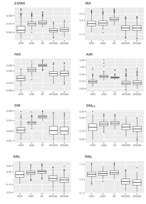
Figure 1. Boxplots of empirical $L_{2}$ errors

6. Concluding remarks

In this paper, we have advanced statistical theory of feed-forward deep neural networks (DNN) for dependent data. For this, we investigated statistical properties of DNN estimators for nonparametric estimation of the mean function of a nonstationary and nonlinear time series. We established generalization error bounds of both non-penalized and sparse-penalized DNN estimators and showed that the sparse-penalized DNN estimators can estimate the mean functions of a wide class of the nonlinear autoregressive (AR) models adaptively and attain the minimax optimal convergence rates up to a logarithmic factor. The class of nonlinear AR models covers nonlinear generalized additive AR, single index models, and popular nonlinear AR models with discontinuous mean functions such as multi-regime threshold AR models.

It would be possible to extend the results in Section 4 to other function classes such as piecewise smooth functions (Imaizumi and Fukumizu, 2019), functions with low intrinsic dimensions (Schmidt-Hieber, 2019; Nakada and Imaizumi, 2020), and functions with varying smoothness (Suzuki, 2019; Suzuki and Nitanda, 2021). We leave such extensions as future research.

Appendix A Proofs for Section 3

For random elements $X$ and $Y$, we write $X\stackrel{{\scriptstyle\mathcal{L}}}{{=}}Y$ if they have the same law. Let $\mathcal{F}$ be a pointwise measurable class of real-valued functions on $\mathbb{R}^{d}$. For $\delta>0$, a finite set $\mathcal{G}\subset\mathcal{F}$ is called a $\delta$-covering of $\mathcal{F}$ with respect to $\|\cdot\|_{\infty}$ if for any $f\in\mathcal{F}$ there exists $g\in\mathcal{G}$ such that $\|f-g\|_{\infty}\leq\delta$. The minimum cardinality of a $\delta$-covering of $\mathcal{F}$ with respect to $\|\cdot\|_{\infty}$ is called the covering number of $\mathcal{F}$ with respect to $\|\cdot\|_{\infty}$ and denoted by $N(\delta,\mathcal{F},\|\cdot\|_{\infty})$. Let $\sigma(Z)$ be the $\sigma$-field generated by the random element $Z$. Let $\widehat{f}_{T}$ be an estimator taking values in $\mathcal{F}$ and define its expected empirical error by

$$\widehat{R}(\widehat{f}_{T},f_{0})=\mathrm{E}\left[{1\over T}\sum_{t=1}^{T}(\widehat{f}_{T}(X_{t})-f_{0}(X_{t}))^{2}\right].$$

In what follows, we set $\beta(t)=\beta_{X}(t)$.

A.1. Proof of Theorem 3.1

First, we give an overview of the proof. To prove Theorem 3.1, we will show the following results:

Lemma A.1 (Lemma C.1).

Let $\delta>0$ and suppose that there exists an integer $\mathcal{N}_{T}$ such that $\mathcal{N}_{T}\geq N(\delta,\mathcal{F},\|\cdot\|_{\infty})\vee\exp(10)$. Also, let $a_{T}$ be a positive number such that $\mu_{T}:=\lfloor T/(2a_{T})\rfloor>0$. In addition, suppose that there is a number $F\geq 1$ such that $\|f\|_{\infty}\leq F$ for all $f\in\mathcal{F}\cup\{f_{0}\}$. Then, for all $\varepsilon\in(0,1]$,

$$R(\widehat{f}_{T},f_{0}) \leq(1+\varepsilon)\widehat{R}(\widehat{f}_{T},f_{0})+{21(1+\varepsilon)^{2}\over\varepsilon}F^{2}{\log\mathcal{N}_{T}\over\mu_{T}}+{4F^{2}\over\mu_{T}}+4(2+\varepsilon)F^{2}\beta(a_{T})+4(2+\varepsilon)F\delta.$$

Lemma A.2 (Lemma C.2).

Let $\{(Y_{t},X_{t})\}_{t=1}^{T}$ be a time series satisfying (2.1), and set $f_{0}:=m\mathbf{1}_{[0,1]^{d}}$. Also, let $\delta>0$ and assume $\mathcal{N}_{T}:=N(\delta,\mathcal{F},\|\cdot\|_{\infty})<\infty$. Suppose that there is a number $F\geq 1$ such that $\|f\|_{\infty}\leq F$ for all $f\in\mathcal{F}\cup\{f_{0}\}$. Suppose also that $\operatorname{supp}(f)\subset[0,1]^{d}$ for all $f\in\mathcal{F}$. Then, under Assumption 3.1, for all $\varepsilon\in(0,1)$ there exists a constant $C_{\varepsilon}$ depending only on $(C_{\eta},\varepsilon,K)$ such that

$$\widehat{R}(\widehat{f}_{T},f_{0}) \leq{1\over 1-\varepsilon}\Psi_{T}^{\mathcal{F}}(\widehat{f}_{T})+{1\over 1-\varepsilon}\inf_{f\in\mathcal{F}}R(f,f_{0})+C_{\varepsilon}F^{2}\gamma_{\delta,T},$$

where

$$\gamma_{\delta,T}:=\delta+{(\log T)(\log\mathcal{N}_{T})\over T}+{1\over T}.$$

Combining these results, we have

$$R(\widehat{f}_{T},f_{0}) \leq{1+\varepsilon\over 1-\varepsilon}\left(\Psi^{\mathcal{F}}(\widehat{f}_{T})+\inf_{f\in\mathcal{F}}R(f,f_{0})\right)$$

$$\quad+C_{\varepsilon}(1+\varepsilon)F^{2}\left(\delta+{(\log T)(\log\mathcal{N}_{T})\over T}+{1\over T}\right)+{21(1+\varepsilon)^{2}F^{2}\over\varepsilon}{\log\mathcal{N}_{T}\over\mu_{T}}+{4F^{2}\over\mu_{T}}$$

$$\quad+4(2+\varepsilon)F^{2}\beta(a_{T})+4(2+\varepsilon)F\delta,$$ (A.1)

where $C_{\varepsilon}$ is a constant depending only on $(\varepsilon,C_{\eta},K)$. Lemma C.1 provides a bound of the generalization error using the expected empirical error and Lemma C.2 provides a bound of the expected empirical error. Note that the results do not require the estimator $\widehat{f}_{T}$ to take values in $\mathcal{F}_{\sigma}(L,N,B,F,S)$ and hence would be of independent interest. Lemma C.1 can be shown as follows: Firstly, we apply the blocking technique for $\beta$-mixing sequences in Rio (2013) to approximate the data with independent blocks. Then, we employ an approach similar to Lemma 4(I) in Schmidt-Hieber (2020) for these independent blocks. In this bound, what distinguishes it from independent data is that the second and third terms come from the blocking argument, while the fourth term depends on the $\beta$-mixing coefficient. When the data is independent, corresponding to $\mu_{T}=T$ and $\beta(a_{T})=0$, this bound corresponds to Lemma 4(I) in Schmidt-Hieber (2020). Lemma C.2 corresponds to Lemma 4(III) in Schmidt-Hieber (2020). Although the bound in Lemma C.2 does not explicitly manifest the time-series structure, a key aspect of the proof involves establishing a new exponential inequality for self-normalized martingale differences (Lemma D.3) and using this result to evaluate $\mathrm{E}[T^{-1}\sum_{t=1}^{T}(\widehat{f}_{T}(X_{t})-f_{0}(X_{t}))\eta(X_{t})v_{t}]$. This approach differs from Schmidt-Hieber (2020) and constitutes a unique aspect of the proof. Theorem 3.1 follows from these lemmas and the bound on the $T^{-1}$-covering number of $\mathcal{F}_{\sigma}(L,N,B,F,S)$ with respect to $\|\cdot\|_{\infty}$.

Now we move on to the proof of Theorem 3.1. Letting $\mathcal{F}=\mathcal{F}_{\sigma}(L,N,B,F,S)$, $\delta=T^{-1}$ and $a_{T}=C_{2,\beta}^{-1}\log T$ in (A.1), we have

$$R(\widehat{f}_{T},f_{0}) \leq{1+\varepsilon\over 1-\varepsilon}\Psi_{T}^{\mathcal{F}}(\widehat{f}_{T})+{1+\varepsilon\over 1-\varepsilon}\inf_{f\in\mathcal{F}}R(f,f_{0})+\left({21(1+\varepsilon)^{2}\over\varepsilon}\log\mathcal{N}_{T}+4\right){F^{2}\over\mu_{T}}$$

$$\quad+\left(2C_{\varepsilon}(1+\varepsilon)+8(2+\varepsilon)\right){F^{2}\over T}+C_{\varepsilon}(1+\varepsilon)F^{2}{(\log T)(\log\mathcal{N}_{T})\over T}.$$

We may assume $\mu_{T}=\lfloor{T\over 2a_{T}}\rfloor>0$; otherwise $T<2a_{T}$ and thus $C_{2,\beta}/2<{\log T\over T}$. Moreover, using Lemma E.5, $\log N\left(T^{-1},\mathcal{F}_{\sigma}(L,N,B,F,S),\|\cdot\|_{\infty}\right)\leq 2S(L+1)\log\left((L+1)(N+1)BT\right)$. Therefore, letting $\mathcal{N}_{T}:=N\left(T^{-1},\mathcal{F}_{\sigma}(L,N,B,F,S),\|\cdot\|_{\infty}\right)\vee\exp(10)$, there exists a universal constant $c_{1}>0$ such that $\log\mathcal{N}_{T}\leq c_{1}S(L+1)\log\left((L+1)(N+1)BT\right)$. Combining all the estimates above, we obtain the desired result. ∎

Remark A.1 (Derivation of (3.4)).

When the $\beta$-mixing coefficient decays polynomially fast, that is, $\beta(t)\leq C_{\beta}t^{-\alpha}$ for some $\alpha>0$, then letting $\delta=T^{-1}$ and $a_{T}=(T/\log\mathcal{N}_{T})^{{1\over\alpha+1}}$ in (A.1), we obtain (3.4).

A.2. Proof of Theorem 3.2

Throughout the proof, we set $\beta(t)=\beta_{X}(t)$. Without loss of generality, we may assume $(1+C_{\tau})T^{-1}<1$; otherwise, the desired bound holds with $C=4(1+C_{\tau})$ because $R(\widehat{f}_{T},f_{0})\leq 4F^{2}$. Then we have

$$\delta_{T}:=T^{-1}+\tau_{T}(L_{T}+1)((N_{T}+1)B_{T})^{L_{T}+1}\leq(1+C_{\tau})T^{-1}<1.$$ (A.2)

Next, for $k\geq 0$ and $s>0$, we define $\mathcal{F}_{T,k,s}:=\left\{f\in\mathcal{F}:2^{k-1}s\mathbf{1}_{\{k\neq 0\}}\leq J_{T}(f)<2^{k}s\right\}$, $\Omega_{T,k,s}:=\left\{\widehat{f}_{T}\in\mathcal{F}_{T,k,s}\right\}$. Note that $\Omega=\bigcup_{k=0}^{\infty}\Omega_{T,k,s}$ and $\Omega_{T,k_{1},s}\cap\Omega_{T,k_{2},s}=\emptyset$ for $k_{1}\neq k_{2}$. For each $k$, set $\mathcal{N}_{k}:=N(\delta_{T},\mathcal{F}_{T,k,s},\|\cdot\|_{\infty})$ and let $\{f^{k}_{1},\dots,f^{k}_{\mathcal{N}_{k}}\}$ be a $\delta_{T}$-covering of $\mathcal{F}_{T,k,s}$ with respect to $\|\cdot\|_{\infty}$. By construction, we can define a random variable $J_{k}$ taking values in $\{1,\dots,\mathcal{N}_{k}\}$ such that $\|\widehat{f}_{T}-f^{k}_{J_{k}}\|_{\infty}\leq\delta_{T}$ on $\Omega_{T,k,s}$.

Step 1 (Reduction to independence) Let $a_{T}$ be a positive number such that $2a_{T}<T$, $a_{T}\to\infty$ and $a_{T}/\iota_{\lambda}(T)\to 0$ as $T\to\infty$, and set $\mu_{T}:=\lfloor T/2a_{T}\rfloor>0$. For $\ell=0,\dots,\mu_{T}-1$, let $I_{1,\ell}=\{2\ell a_{T}+1,\dots,(2\ell+1)a_{T}\}$, $I_{2,\ell}=\{(2\ell+1)a_{T}+1,\dots,2(\ell+1)a_{T}\}$. For each $k$, we define

$$\widetilde{g}^{k}_{\ell} :=(\widetilde{g}^{k}_{1,\ell},\dots,\widetilde{g}^{k}_{\mathcal{N}_{k},\ell})^{\prime}=\left(\sum_{t\in I_{1,\ell}}(f^{k}_{1}(X_{t})-f_{0}(X_{t}))^{2},\dots,\sum_{t\in I_{1,\ell}}(f^{k}_{\mathcal{N}_{k}}(X_{t})-f_{0}(X_{t}))^{2}\right)^{\prime},$$

$$\widetilde{g}_{\ell}^{\ast,k} :=(\widetilde{g}_{1,\ell}^{\ast,k},\dots,\widetilde{g}_{\mathcal{N}_{k},\ell}^{\ast,k})^{\prime}=\left(\sum_{t\in I_{1,\ell}}(f^{k}_{1}(X_{t}^{\ast})-f_{0}(X_{t}^{\ast}))^{2},\dots,\sum_{t\in I_{1,\ell}}(f^{k}_{\mathcal{N}_{k}}(X_{t}^{\ast})-f_{0}(X_{t}^{\ast}))^{2}\right)^{\prime}.$$

From a similar argument in Step1 of the proof of Lemma C.1, we can show that there exist two sequences of independent $\mathbb{R}^{\mathcal{N}_{k}}$-valued random variables $\{g_{\ell}^{k}\}_{\ell=0}^{\mu_{T}-1}$ and $\{g_{\ell}^{\ast,k}\}_{\ell=0}^{\mu_{T}-1}$ such that for all $\ell=0,\dots,\mu_{T}-1$,

$$g^{k}_{\ell} \stackrel{{\scriptstyle\mathcal{L}}}{{=}}\widetilde{g}^{k}_{\ell},\ \operatorname{P}(g^{k}_{\ell}\neq\widetilde{g}^{k}_{\ell})\leq\beta(a_{T}),\quad g^{\ast,k}_{\ell}\stackrel{{\scriptstyle\mathcal{L}}}{{=}}\widetilde{g}^{\ast,k}_{\ell},\ \operatorname{P}(g^{\ast,k}_{\ell}\neq\widetilde{g}^{\ast,k}_{\ell})\leq\beta(a_{T}).$$

with $0\leq g^{k}_{j,\ell}\leq 4F^{2}a_{T}$ and $0\leq g^{\ast,k}_{j,\ell}\leq 4F^{2}a_{T}$ a.s., where $g^{k}_{j,\ell}$ and $g_{j,\ell}^{\ast,k}$ are the $j$-th components of $g^{k}_{\ell}$ and $g_{\ell}^{\ast,k}$, respectively. Further, let $k_{T,s}$ be an integer such that $\sum_{k\geq k_{T,s}+1}\operatorname{P}(\Omega_{T,k,s})\leq 1/\mu_{T}$. For $\ell=0,\dots,\mu_{T}-1$, we define

$$\widetilde{\mathfrak{g}}_{\ell} :=\left((\widetilde{g}^{0}_{\ell})^{\prime},\dots,(\widetilde{g}^{k_{T,s}}_{\ell})^{\prime}\right)^{\prime},\ \widetilde{\mathfrak{g}}^{\ast}_{\ell}:=\left((\widetilde{g}^{\ast,0}_{\ell})^{\prime},\dots,(\widetilde{g}^{\ast,k_{T,s}}_{\ell})^{\prime}\right)^{\prime},$$

$$\mathfrak{g}_{\ell} :=\left((g^{0}_{\ell})^{\prime},\dots,(g^{k_{T,s}}_{\ell})^{\prime}\right)^{\prime},\ \mathfrak{g}^{\ast}_{\ell}:=\left((g^{\ast,0}_{\ell})^{\prime},\dots,(g^{\ast,k_{T,s}}_{\ell})^{\prime}\right)^{\prime}.$$

We can also assume that for all $\ell=0,\dots,\mu_{T}-1$,

$$\mathfrak{g}_{\ell} \stackrel{{\scriptstyle\mathcal{L}}}{{=}}\widetilde{\mathfrak{g}}_{\ell},\ \operatorname{P}(\mathfrak{g}_{\ell}\neq\widetilde{\mathfrak{g}}_{\ell})\leq\beta(a_{T}),\quad\mathfrak{g}^{\ast}_{\ell}\stackrel{{\scriptstyle\mathcal{L}}}{{=}}\widetilde{\mathfrak{g}}^{\ast}_{\ell},\ \operatorname{P}(\mathfrak{g}^{\ast}_{\ell}\neq\widetilde{\mathfrak{g}}^{\ast}_{\ell})\leq\beta(a_{T}).$$

Likewise, define

$$\widetilde{h}^{k}_{\ell} :=(\widetilde{h}^{k}_{1,\ell},\dots,\widetilde{h}^{k}_{\mathcal{N}_{k},\ell})=\left(\sum_{t\in I_{2,\ell}}(f^{k}_{1}(X_{t})-f_{0}(X_{t}))^{2},\dots,\sum_{t\in I_{2,\ell}}(f^{k}_{\mathcal{N}_{k}}(X_{t})-f_{0}(X_{t}))^{2}\right)^{\prime},$$

$$\widetilde{h}_{\ell}^{\ast,k} :=(\widetilde{h}_{1,\ell}^{\ast,k},\dots,\widetilde{h}_{\mathcal{N}_{k},\ell}^{\ast,k})=\left(\sum_{t\in I_{2,\ell}}(f^{k}_{1}(X_{t}^{\ast})-f_{0}(X_{t}^{\ast}))^{2},\dots,\sum_{t\in I_{2,\ell}}(f^{k}_{\mathcal{N}_{k}}(X_{t}^{\ast})-f_{0}(X_{t}^{\ast}))^{2}\right)^{\prime}$$

and there exist two sequences of independent $\mathbb{R}^{\mathcal{N}_{k}}$-valued random variables $\{h_{\ell}^{k}\}_{\ell=0}^{\mu_{T}-1}$ and $\{h_{\ell}^{\ast,k}\}_{\ell=0}^{\mu_{T}-1}$ such that for all $\ell=0,\dots,\mu_{T}-1$,

$$h^{k}_{\ell} \stackrel{{\scriptstyle\mathcal{L}}}{{=}}\widetilde{h}^{k}_{\ell},\ \operatorname{P}(h^{k}_{\ell}\neq\widetilde{h}^{k}_{\ell})\leq\beta(a_{T}),\quad h^{\ast,k}_{\ell}\stackrel{{\scriptstyle\mathcal{L}}}{{=}}\widetilde{h}^{\ast,k}_{\ell},\ \operatorname{P}(h^{\ast,k}_{\ell}\neq\widetilde{h}^{\ast,k}_{\ell})\leq\beta(a_{T}).$$

For $\ell=0,\dots,\mu_{T}-1$, we define

$$\widetilde{\mathfrak{h}}_{\ell} :=\left((\widetilde{h}^{0}_{\ell})^{\prime},\dots,(\widetilde{h}^{k_{T,s}}_{\ell})^{\prime}\right)^{\prime},\ \widetilde{\mathfrak{h}}^{\ast}_{\ell}:=\left((\widetilde{h}^{\ast,0}_{\ell})^{\prime},\dots,(\widetilde{h}^{\ast,k_{T,s}}_{\ell})^{\prime}\right)^{\prime},$$

$$\mathfrak{h}_{\ell} :=\left((h^{0}_{\ell})^{\prime},\dots,(h^{k_{T,s}}_{\ell})^{\prime}\right)^{\prime},\ \mathfrak{h}^{\ast}_{\ell}:=\left((h^{\ast,0}_{\ell})^{\prime},\dots,(h^{\ast,k_{T,s}}_{\ell})^{\prime}\right)^{\prime}.$$

We can also assume that for all $\ell=0,\dots,\mu_{T}-1$,

$$\mathfrak{h}_{\ell} \stackrel{{\scriptstyle\mathcal{L}}}{{=}}\widetilde{\mathfrak{h}}_{\ell},\ \operatorname{P}(\mathfrak{h}_{\ell}\neq\widetilde{\mathfrak{h}}_{\ell})\leq\beta(a_{T}),\quad\mathfrak{h}^{\ast}_{\ell}\stackrel{{\scriptstyle\mathcal{L}}}{{=}}\widetilde{\mathfrak{h}}^{\ast}_{\ell},\ \operatorname{P}(\mathfrak{h}^{\ast}_{\ell}\neq\widetilde{\mathfrak{h}}^{\ast}_{\ell})\leq\beta(a_{T}).$$

Step 2 (Bounding the generalization error) In this step, we will show

$$R(\widehat{f}_{T},f_{0}) \leq 3\left(\widehat{R}(\widehat{f}_{T},f_{0})+{1\over 3}\mathrm{E}[J_{T}(\widehat{f}_{T})]\right)+{32F^{2}a_{T}\over T}\left(1+{2^{5/4}\exp\left(-{sT\over 128F^{2}a_{T}}\right)\over 1-\exp\left(-{sT\over 256F^{2}a_{T}}\right)}\right)$$

$$\quad\quad+24F\delta_{T}+{s\over 4}+{32F^{2}\over\mu_{T}}+48F^{2}\beta(a_{T})$$ (A.3)

for $T\geq T_{0}$, where $T_{0}>0$ is a constant depending only on ($C_{L}$, $C_{N}$, $C_{B}$, $\nu_{0}$, $\nu_{1}$, $\nu_{2}$, $\iota_{\lambda}$). Define

$$D :=R(\widehat{f}_{T},f_{0})-\widehat{R}(\widehat{f}_{T},f_{0})-{1\over 2}\mathrm{E}[J_{T}(\widehat{f}_{T})],\ D_{k}:=\mathrm{E}\left[\mathbf{1}_{\Omega_{T,k,s}}\left({1\over T}\sum_{t=1}^{T}\Delta_{t}(\widehat{f}_{T})-{1\over 2}J_{T}(\widehat{f}_{T})\right)\right],$$

where $\Delta_{t}(f)=(f(X_{t}^{\ast})-f_{0}(X_{t}^{\ast}))^{2}-(f(X_{t})-f_{0}(X_{t}))^{2}$. Note that $D=\sum_{k=0}^{\infty}D_{k}$. Since $|\Delta_{t}(\widehat{f}_{T})-\Delta_{t}(f_{J_{k}}^{k})|\leq 8F\delta_{T}$, we have

$$D_{k} \leq\mathrm{E}\left[\mathbf{1}_{\Omega_{T,k,s}}\left({1\over T}\sum_{t=1}^{T}\Delta_{t}(f_{J_{k}}^{k})-{1\over 2}J_{T}(\widehat{f}_{T})\right)\right]+\mathrm{E}\left[\mathbf{1}_{\Omega_{T,k,s}}\left({1\over T}\sum_{t=1}^{T}\left|\Delta_{t}(\widehat{f}_{T})-\Delta_{t}(f_{J_{k}}^{k})\right|\right)\right]$$

$$\leq\mathrm{E}\left[\mathbf{1}_{\Omega_{T,k,s}}\left({1\over T}\sum_{t=1}^{T}\Delta_{t}(f_{J_{k}}^{k})-{1\over 2}J_{T}(\widehat{f}_{T})\right)\right]+8F\delta_{T}\operatorname{P}(\Omega_{T,k,s}).$$

Observe that

$$\mathrm{E}\left[\mathbf{1}_{\Omega_{T,k,s}}\left({1\over T}\sum_{t=1}^{T}\Delta_{t}(f_{J_{k}}^{k})\right)\right]$$

$$\leq\mathrm{E}\left[\mathbf{1}_{\Omega_{T,k,s}}{1\over T}\!\left(\sum_{\ell=0}^{\mu_{T}-1}\widetilde{g}_{J_{k},\ell}^{\ast,k}+\!\!\sum_{\ell=0}^{\mu_{T}-1}\widetilde{h}_{J_{k},\ell}^{\ast,k}-\!\!\sum_{\ell=0}^{\mu_{T}-1}\widetilde{g}_{J_{k},\ell}^{k}-\!\!\sum_{\ell=0}^{\mu_{T}-1}\widetilde{h}_{J_{k},\ell}^{k}\right)\!\right]\!+\!\mathrm{E}\left[\mathbf{1}_{\Omega_{T,k,s}}\!\left(\!{1\over T}\sum_{t=2a_{T}\mu_{T}+1}^{T}\!\!\!\!\!\!\!\!|\Delta_{t}(f^{k}_{J_{k}})|\!\right)\right]$$

$$\leq\mathrm{E}\left[\mathbf{1}_{\Omega_{T,k,s}}{1\over T}\!\left(\sum_{\ell=0}^{\mu_{T}-1}\widetilde{g}_{J_{k},\ell}^{\ast,k}+\!\!\sum_{\ell=0}^{\mu_{T}-1}\widetilde{h}_{J_{k},\ell}^{\ast,k}-\!\!\sum_{\ell=0}^{\mu_{T}-1}\widetilde{g}_{J_{k},\ell}^{k}-\!\!\sum_{\ell=0}^{\mu_{T}-1}\widetilde{h}_{J_{k},\ell}^{k}\right)\!\right]+{8F^{2}\over\mu_{T}}\operatorname{P}(\Omega_{T,k,s}).$$

Further,

$${1\over T}\sum_{\ell=0}^{\mu_{T}-1}\sum_{k=0}^{\infty}\mathrm{E}\left[\mathbf{1}_{\Omega_{T,k,s}}\left|\widetilde{g}_{J_{k},\ell}^{\ast,k}-g_{J_{k},\ell}^{\ast,k}\right|\right]\leq{4F^{2}a_{T}\over T}\sum_{\ell=0}^{\mu_{T}-1}\sum_{k=0}^{\infty}\mathrm{E}\left[\mathbf{1}_{\Omega_{T,k,s}}\mathbf{1}_{\left\{\widetilde{g}_{J_{k},\ell}^{\ast,k}\neq g_{J_{k},\ell}^{\ast,k}\right\}}\right]$$

$$\leq{4F^{2}a_{T}\over T}\sum_{\ell=0}^{\mu_{T}-1}\sum_{k=0}^{\infty}\mathrm{E}\left[\mathbf{1}_{\Omega_{T,k,s}}\mathbf{1}_{\left\{\mathfrak{\widetilde{g}}_{\ell}^{\ast}\neq\mathfrak{g}_{\ell}^{\ast}\right\}}\right]\leq{4F^{2}a_{T}\over T}\sum_{\ell=0}^{\mu_{T}-1}\!\left(\sum_{k=0}^{k_{T,s}}\mathrm{E}\left[\mathbf{1}_{\Omega_{T,k,s}}\mathbf{1}_{\left\{\mathfrak{\widetilde{g}}_{\ell}^{\ast}\neq\mathfrak{g}_{\ell}^{\ast}\right\}}\right]+\sum_{k=k_{T,s}+1}^{\infty}\!\!\!\!\!\mathrm{E}\left[\mathbf{1}_{\Omega_{T,k,s}}\right]\!\right)$$

$$\leq{4F^{2}a_{T}\over T}\sum_{\ell=0}^{\mu_{T}-1}\!\left(\mathrm{E}\left[\mathbf{1}_{\left\{\mathfrak{\widetilde{g}}_{\ell}^{\ast}\neq\mathfrak{g}_{\ell}^{\ast}\right\}}\right]\!+\!\!\sum_{k=k_{T,s}+1}^{\infty}\!\!\!\!\!\mathrm{E}\left[\mathbf{1}_{\Omega_{T,k,s}}\right]\!\right)\leq{4F^{2}a_{T}\over T}\cdot\mu_{T}\left(\beta(a_{T})+\frac{1}{\mu_{T}}\right)\leq 2F^{2}\left(\beta(a_{T})+\frac{1}{\mu_{T}}\right).$$ (A.4)

Therefore, similar arguments to obtain (A.2) yield

$$\sum_{k=0}^{\infty}\mathrm{E}\left[\mathbf{1}_{\Omega_{T,k,s}}\left({1\over T}\sum_{t=1}^{T}\Delta_{t}(f_{J_{k}}^{k})-{1\over 2}J_{T}(\widehat{f}_{T})\right)\right]$$

$$\leq\sum_{k=0}^{\infty}\!\mathrm{E}\!\left[\!\mathbf{1}_{\Omega_{T,k,s}}\!\!\left(\!{1\over T}\!\!\sum_{\ell=0}^{\mu_{T}-1}\!\!\!(g_{J_{k},\ell}^{\ast,k}\!-\!g_{J_{k},\ell}^{k})\!-\!{1\over 4}J_{T}(\widehat{f}_{T})\!\right)\!\right]$$

$$\quad\!+\!\sum_{k=0}^{\infty}\!\mathrm{E}\!\left[\!\mathbf{1}_{\Omega_{T,k,s}}\!\left(\!{1\over T}\!\!\sum_{\ell=0}^{\mu_{T}-1}\!\!\!(h_{J_{k},\ell}^{\ast,k}\!-\!h_{J_{k},\ell}^{k})\!-\!{1\over 4}J_{T}(\widehat{f}_{T})\!\right)\!\right]\!+\!{16F^{2}\over\mu_{T}}\!+\!8F^{2}\beta(a_{T}).$$

Define $b_{j,k}:=\mathbf{1}_{\Omega_{T,k,s}}\sum_{\ell=0}^{\mu_{T}-1}(g_{j,\ell}^{\ast,k}-g_{j,\ell}^{k})^{2}$, $\bar{b}_{k}:=\mathrm{E}\left[b_{J_{k},k}\right]$, $r_{j,k}:=2\sqrt{b_{j,k}+\bar{b}_{k}}$,
$B_{j,k}:=\mathbf{1}_{\Omega_{T,k,s}}\left|\sum_{\ell=0}^{\mu_{T}-1}(g_{j,\ell}^{\ast,k}-g_{j,\ell}^{k})/r_{j,k}\right|$, $B_{k}:=B_{J_{k},k}$, where $B_{j,k}:=0$ if the denominator equals $0$. Then we have

$$\mathrm{E}\left[\mathbf{1}_{\Omega_{T,k,s}}\left({1\over T}\sum_{\ell=0}^{\mu_{T}-1}(g_{J_{k},\ell}^{\ast,k}-g_{J_{k},\ell}^{k})-{1\over 4}J_{T}(\widehat{f}_{T})\right)\right] \leq\mathrm{E}\left[\left({1\over T}r_{J_{k},k}B_{k}-\mathbf{1}_{\Omega_{T,k,s}}{1\over 4}J_{T}(\widehat{f}_{T})\right)\right].$$

Applying the AM-GM inequality, we have

$$\mathrm{E}\!\left[\!\mathbf{1}_{\Omega_{T,k,s}}\!\!\left({1\over T}\!\sum_{\ell=0}^{\mu_{T}-1}\!\!(g_{J_{k},\ell}^{\ast,k}-g_{J_{k},\ell}^{k})\!-\!{1\over 4}J_{T}(\widehat{f}_{T})\!\right)\right]\leq\mathrm{E}\left[{r^{2}_{J_{k},k}\over 64F^{2}Ta_{T}}\right]+\mathrm{E}\left[{16F^{2}a_{T}\over T}B_{k}^{2}-\mathbf{1}_{\Omega_{T,k,s}}{1\over 4}J_{T}(\widehat{f}_{T})\right]$$

$$={8\over 64F^{2}Ta_{T}}\mathrm{E}\left[b_{J_{k},k}\right]\!+\!\mathrm{E}\!\left[\!{16F^{2}a_{T}\over T}B_{k}^{2}\!-\!\mathbf{1}_{\Omega_{T,k,s}}{1\over 4}J_{T}(\widehat{f}_{T})\right]=:I_{r,k}+I_{B,k}.$$

Now we evaluate $I_{r,k}$. Observe that

$$\mathrm{E}[b_{J_{k},k}]$$

$$\leq 4F^{2}a_{T}\mathrm{E}\left[\mathbf{1}_{\Omega_{T,k,s}}\sum_{\ell=0}^{\mu_{T}-1}\left|g_{J_{k},\ell}^{\ast,k}-g_{J_{k},\ell}^{k}\right|\right]$$

$$\leq 4F^{2}a_{T}\mathrm{E}\left[\mathbf{1}_{\Omega_{T,k,s}}\sum_{\ell=0}^{\mu_{T}-1}\left|\widetilde{g}_{J_{k},\ell}^{\ast,k}-\widetilde{g}_{J_{k},\ell}^{k}\right|\right]+4F^{2}a_{T}\mathrm{E}\left[\mathbf{1}_{\Omega_{T,k,s}}\sum_{\ell=0}^{\mu_{T}-1}\left(\left|\widetilde{g}_{J_{k},\ell}^{\ast,k}-g_{J_{k},\ell}^{\ast,k}\right|+\left|\widetilde{g}_{J_{k},\ell}^{k}-g_{J_{k},\ell}^{k}\right|\right)\right]$$

$$\leq 4F^{2}a_{T}\left(\mathrm{E}\left[\mathbf{1}_{\Omega_{T,k,s}}\sum_{\ell=0}^{\mu_{T}-1}\!\!\sum_{t\in I_{1,\ell}}(\widehat{f}_{T}(X_{t}^{\ast})-f_{0}(X_{t}^{\ast}))^{2}\right]+\mathrm{E}\left[\mathbf{1}_{\Omega_{T,k,s}}\sum_{\ell=0}^{\mu_{T}-1}\sum_{t\in I_{1,\ell}}(\widehat{f}_{T}(X_{t})-f_{0}(X_{t}))^{2}\right]\right)$$

$$\ +\!4F^{2}a_{T}\!\left(\!\mathrm{E}\!\left[\!\mathbf{1}_{\Omega_{T,k,s}}\!\!\!\!\sum_{\ell=0}^{\mu_{T}-1}\!\left|\widetilde{g}_{J_{k},\ell}^{\ast,k}\!-\!\!\sum_{t\in I_{1,\ell}}\!\!\!\!(\widehat{f}_{T}(X_{t}^{\ast})\!-\!f_{0}(X_{t}^{\ast})\!)^{2}\right|\right]\!+\!\mathrm{E}\!\left[\!\mathbf{1}_{\Omega_{T,k,s}}\!\!\!\!\sum_{\ell=0}^{\mu_{T}-1}\!\left|\widetilde{g}_{J_{k},\ell}^{k}\!-\!\!\sum_{t\in I_{1,\ell}}\!\!\!\!(\widehat{f}_{T}(X_{t})\!-\!f_{0}(X_{t})\!)^{2}\right|\right]\!\right)$$

$$\ +\!4F^{2}a_{T}\cdot 8F^{2}a_{T}\sum_{\ell=0}^{\mu_{T}-1}\mathrm{E}\left[\mathbf{1}_{\Omega_{T,k,s}}\left(\mathbf{1}_{\left\{\widetilde{g}_{J_{k},\ell}^{\ast,k}\neq g_{J_{k},\ell}^{\ast,k}\right\}}+\mathbf{1}_{\left\{\widetilde{g}_{J_{k},\ell}^{k}\neq g_{J_{k},\ell}^{k}\right\}}\right)\right]$$

$$\leq 4F^{2}a_{T}\mathrm{E}\left[\mathbf{1}_{\Omega_{T,k,s}}\sum_{\ell=0}^{\mu_{T}-1}\!\!\sum_{t\in I_{1,\ell}}(\widehat{f}_{T}(X_{t}^{\ast})-f_{0}(X_{t}^{\ast}))^{2}\right]+4F^{2}a_{T}\mathrm{E}\left[\mathbf{1}_{\Omega_{T,k,s}}\sum_{\ell=0}^{\mu_{T}-1}\!\!\sum_{t\in I_{1,\ell}}(\widehat{f}_{T}(X_{t})-f_{0}(X_{t}))^{2}\right]$$

$$\ +\!4F^{2}\!a_{T}\!\left(4Fa_{T}\mu_{T}\delta_{T}\!+\!4Fa_{T}\mu_{T}\delta_{T}\right)\!\operatorname{P}(\Omega_{T,k,s})\!+\!32F^{4}\!a_{T}^{2}\!\!\!\sum_{\ell=0}^{\mu_{T}-1}\!\!\!\mathrm{E}\!\left[\!\mathbf{1}_{\Omega_{T,k,s}}\!\!\left(\!\mathbf{1}_{\left\{\widetilde{g}_{J_{k},\ell}^{\ast,k}\neq g_{J_{k},\ell}^{\ast,k}\right\}}\!\!+\!\mathbf{1}_{\left\{\widetilde{g}_{J_{k},\ell}^{k}\neq g_{J_{k},\ell}^{k}\right\}}\!\right)\!\right].$$ (A.5)

For the above inequalities, we used the fact that $\left|\widetilde{g}_{J_{k},\ell}^{\ast,k}-g_{J_{k},\ell}^{\ast,k}\right|\leq 4F^{2}a_{T}$, $\left|\widetilde{g}_{J_{k},\ell}^{k}-g_{J_{k},\ell}^{k}\right|\leq 4F^{2}a_{T}$ a.s. and on $\Omega_{T,k,s}$, $\widehat{f}_{T}\in\mathcal{F}_{T,k,s}$ and

$$\left|(f^{k}_{J_{k}}(x)-f_{0}(x))^{2}-(\widehat{f}_{T}(x)-f_{0}(x))^{2}\right| \leq\left|\widehat{f}_{T}(x)-f^{k}_{J_{k}}(x)\right|\left|\widehat{f}_{T}(x)+f^{k}_{J_{k}}(x)-2f_{0}(x)\right|\leq 4F\delta_{T}.$$

Hence we obtain

$$\sum_{k=0}^{\infty}I_{r,k} \leq{4F^{2}a_{T}\over 8F^{2}Ta_{T}}\left(\mathrm{E}\left[\sum_{\ell=0}^{\mu_{T}-1}\sum_{t\in I_{1,\ell}}(\widehat{f}_{T}(X_{t}^{\ast})-f_{0}(X_{t}^{\ast}))^{2}\right]+\mathrm{E}\left[\sum_{\ell=0}^{\mu_{T}-1}\sum_{t\in I_{1,\ell}}(\widehat{f}_{T}(X_{t})-f_{0}(X_{t}))^{2}\right]\right)$$

$$\quad+{32F^{3}a_{T}^{2}\mu_{T}\delta_{T}\over 8F^{2}Ta_{T}}+{32F^{4}\cdot 4a_{T}^{2}\mu_{T}\beta(a_{T})\over 8F^{2}Ta_{T}}$$

$$={1\over 2}\left(\mathrm{E}\left[{1\over T}\sum_{\ell=0}^{\mu_{T}-1}\sum_{t\in I_{1,\ell}}(\widehat{f}_{T}(X_{t}^{\ast})-f_{0}(X_{t}^{\ast}))^{2}\right]+\mathrm{E}\left[{1\over T}\sum_{\ell=0}^{\mu_{T}-1}\sum_{t\in I_{1,\ell}}(\widehat{f}_{T}(X_{t})-f_{0}(X_{t}))^{2}\right]\right)$$

$$\quad+2F\delta_{T}+8F^{2}\beta(a_{T}).$$ (A.6)

Now we evaluate $I_{B,k}$. If $\bar{b}_{k}>0$, applying Lemmas E.2 and E.4 with $y=\sqrt{\bar{b}_{k}}$, we obtain $\mathrm{E}\left[\exp\left(2B_{j,k}^{2}\right)\sqrt{\bar{b}_{k}}/\sqrt{b_{j,k}+\bar{b}_{k}}\right]\leq 1$. Hence

$$\mathrm{E}\left[\exp\left(2B_{J_{k},k}^{2}\right)\sqrt{\bar{b}_{k}}/\sqrt{b_{J_{k},k}+\bar{b}_{k}}\right]\leq\mathrm{E}\left[\max_{1\leq j\leq\mathcal{N}_{k}}\exp\left(2B_{j,k}^{2}\right)\sqrt{\bar{b}_{k}}/\sqrt{b_{j,k}+\bar{b}_{k}}\right]\leq\mathcal{N}_{k}.$$

Therefore, by the Cauchy-Schwarz inequality, we obtain

$$\operatorname{E}[\exp(B_{k}^{2})]\!\leq\!\sqrt{\mathrm{E}\!\left[\exp\left(\!2B_{J_{k},k}^{2}\!\right)\!\!\sqrt{\bar{b}_{k}}/\!\sqrt{b_{J_{k},k}+\bar{b}_{k}}\right]\!\mathrm{E}\!\left[\!\sqrt{b_{J_{k},k}+\bar{b}_{k}}/\sqrt{\bar{b}_{k}}\right]}\!\leq\!\sqrt{\mathcal{N}_{k}\mathrm{E}\!\left[\!\sqrt{b_{J_{k},k}+\bar{b}_{k}}/\!\sqrt{\bar{b}_{k}}\right]}.$$

Since $\mathrm{E}\left[\sqrt{b_{J_{k},k}+\bar{b}_{k}}/\sqrt{\bar{b}_{k}}\right]\leq\sqrt{\mathrm{E}\left[(b_{J_{k},k}+\bar{b}_{k})/\bar{b}_{k}\right]}\leq\sqrt{2}$, we conclude

$$\operatorname{E}[\exp(B_{k}^{2})]\leq 2^{1/4}\sqrt{\mathcal{N}_{k}}.$$ (A.7)

This inequality also holds when $\bar{b}_{k}=0$ because we always have $B_{k}=0$ in such a case. Thus, for $k\geq 1$, we have

$$\mathrm{E}\left[{16F^{2}a_{T}\over T}B_{k}^{2}-\mathbf{1}_{\Omega_{T,k,s}}{1\over 4}J_{T}(\widehat{f}_{T})\right]\leq\int_{0}^{\infty}\operatorname{P}\left({16F^{2}a_{T}\over T}B_{k}^{2}-\mathbf{1}_{\Omega_{T,k,s}}{1\over 4}J_{T}(\widehat{f}_{T})>x\right)dx$$

$$\leq 2^{1/4}\sqrt{\mathcal{N}_{k}}\int_{0}^{\infty}\exp\left(-{T(x+2^{k-3}s)\over 16F^{2}a_{T}}\right)dx=2^{1/4}\sqrt{\mathcal{N}_{k}}\cdot{16F^{2}a_{T}\over T}\exp\left(-{2^{k-3}sT\over 16F^{2}a_{T}}\right),$$ (A.8)

where the second inequality follows from Markov’s inequality and (A.7). Recall that $\delta_{T}$ is defined by (A.2). Then by Lemma E.6,

$$\log\mathcal{N}_{k}\leq{2^{k}s\over\lambda_{T}}(L_{T}+1)\log\left({(L_{T}+1)(N_{T}+1)B_{T}\over T^{-1}}\right)\leq C_{1}{2^{k}s\over\lambda_{T}}\log^{1+\nu_{0}}T,$$ (A.9)

where $C_{1}$ is a positive constant depending only on ($C_{L}$, $C_{N}$, $C_{B}$, $\nu_{0}$, $\nu_{1}$, $\nu_{2}$). Since $a_{T}/\iota_{\lambda}(T)\to 0$ as $T\to\infty$, there is a constant $T_{0}$ depending only on $C_{1}$ and $\iota_{\lambda}$ such that $(C_{1}\log^{1+\nu_{0}}T)/\lambda_{T}\leq T/(128F^{2}a_{T})$ whenever $T\geq T_{0}$. For such $T$, we have

$$2^{1/4}\sqrt{\mathcal{N}_{k}}\cdot{16F^{2}a_{T}\over T}\exp\left(-{2^{k-3}sT\over 16F^{2}a_{T}}\right) \leq{2^{1/4}\cdot 16F^{2}a_{T}\over T}\exp\left({2^{k}sT\over 256F^{2}a_{T}}-{2^{k}sT\over 128F^{2}a_{T}}\right)$$

$$={2^{1/4}\cdot 16F^{2}a_{T}\over T}\exp\left(-{2^{k}sT\over 256F^{2}a_{T}}\right).$$

For $k=0$,

$$\mathrm{E}\left[{16F^{2}a_{T}\over T}B_{0}^{2}-\mathbf{1}_{\Omega_{T,0,s}}{1\over 4}J_{T}(\widehat{f}_{T})\right]\leq{16F^{2}a_{T}\over T}\mathrm{E}[B_{0}^{2}]={16F^{2}a_{T}\over T}\log(\exp(\mathrm{E}[B_{0}^{2}]))$$

$$\leq{16F^{2}a_{T}\over T}\log(\mathrm{E}[\exp(B_{0}^{2})])\leq{16F^{2}a_{T}\over T}\log(2^{1/4}\sqrt{\mathcal{N}_{0}})\leq{8F^{2}a_{T}\over T}(1+\log\mathcal{N}_{0})\leq{8F^{2}a_{T}\over T}+{s\over 16}.$$ (A.10)

For the second inequality, we used Jensen’s inequality and for the last inequality, we used $\log\mathcal{N}_{0}\leq sT/(128F^{2}a_{T})$. Combining (A.2) and (A.2), we have

$$\sum_{k=0}^{\infty}\!I_{B,k} \leq{8F^{2}a_{T}\over T}\!+\!{s\over 16}\!+\!{2^{1/4}\!\cdot\!16F^{2}a_{T}\over T}\sum_{k=1}^{\infty}\exp\left(-{2^{k}sT\over 256F^{2}a_{T}}\right)\leq{s\over 16}\!+\!{8F^{2}a_{T}\over T}\left(\!1\!+\!{2^{5/4}\exp\left(-{sT\over 128F^{2}a_{T}}\right)\over 1-\exp\left(-{sT\over 256F^{2}a_{T}}\right)}\!\right).$$ (A.11)

Therefore, (A.2) and (A.11) yield

$$\sum_{k=0}^{\infty}\mathrm{E}\left[\mathbf{1}_{\Omega_{T,k,s}}\left({1\over T}\sum_{\ell=0}^{\mu_{T}-1}(g_{J_{k},\ell}^{\ast,k}-g_{J_{k},\ell}^{k})-{1\over 4}J_{T}(\widehat{f}_{T})\right)\right]\leq\sum_{k=0}^{\infty}(I_{r,k}+I_{B,k})$$

$$\leq{1\over 2}\left(\mathrm{E}\left[{1\over T}\sum_{\ell=0}^{\mu_{T}-1}\sum_{t\in I_{1,\ell}}(\widehat{f}_{T}(X_{t}^{\ast})-f_{0}(X_{t}^{\ast}))^{2}\right]+\mathrm{E}\left[{1\over T}\sum_{\ell=0}^{\mu_{T}-1}\sum_{t\in I_{1,\ell}}(\widehat{f}_{T}(X_{t})-f_{0}(X_{t}))^{2}\right]\right)$$

$$\quad+2F\delta_{T}+8F^{2}\beta(a_{T})+{s\over 16}+{8F^{2}a_{T}\over T}\left(1+{2^{5/4}\exp\left(-{sT\over 128F^{2}a_{T}}\right)\over 1-\exp\left(-{sT\over 256F^{2}a_{T}}\right)}\right).$$

Likewise, we have

$$\sum_{k=0}^{\infty}\mathrm{E}\left[\mathbf{1}_{\Omega_{T,k,s}}\left({1\over T}\sum_{\ell=0}^{\mu_{T}-1}(h_{J_{k},\ell}^{\ast,k}-h_{J_{k},\ell}^{k})-{1\over 4}J_{T}(\widehat{f}_{T})\right)\right]$$

$$\leq{1\over 2}\left(\mathrm{E}\left[{1\over T}\sum_{\ell=0}^{\mu_{T}-1}\sum_{t\in I_{2,\ell}}(\widehat{f}_{T}(X_{t}^{\ast})-f_{0}(X_{t}^{\ast}))^{2}\right]+\mathrm{E}\left[{1\over T}\sum_{\ell=0}^{\mu_{T}-1}\sum_{t\in I_{2,\ell}}(\widehat{f}_{T}(X_{t})-f_{0}(X_{t}))^{2}\right]\right)$$

$$\quad+2F\delta_{T}+8F^{2}\beta(a_{T})+{s\over 16}+{8F^{2}a_{T}\over T}\left(1+{2^{5/4}\exp\left(-{sT\over 128F^{2}a_{T}}\right)\over 1-\exp\left(-{sT\over 256F^{2}a_{T}}\right)}\right).$$

Hence,

$$D =\sum_{k=1}^{\infty}D_{k}\leq{1\over 2}\left(R(\widehat{f}_{T},f_{0})+\widehat{R}(\widehat{f}_{T},f_{0})\right)$$

$$\quad\quad\quad\quad\quad\!+\!12F\delta_{T}\!+\!16F^{2}\beta(a_{T})\!+\!{s\over 8}\!+\!{16F^{2}a_{T}\over T}\left(1\!+\!{2^{5/4}\exp\left(-{sT\over 128F^{2}a_{T}}\right)\over 1-\exp\left(-{sT\over 256F^{2}a_{T}}\right)}\right)\!+\!{16F^{2}\over\mu_{T}}\!+\!8F^{2}\beta(a_{T}).$$

Since $D=R(\widehat{f}_{T},f_{0})-\widehat{R}(\widehat{f}_{T},f_{0})-{1\over 2}\mathrm{E}[J_{T}(\widehat{f}_{T})]$, we obtain (A.2).

Step 3 (Bounding the expected empirical error) In this step, we will show that for any $\bar{f}\in\mathcal{F}$,

$$\widehat{R}(\widehat{f}_{T},f_{0})+{1\over 3}\mathrm{E}[J_{T}(\widehat{f}_{T})] \leq 2\left(\bar{\Psi}_{T}(\widehat{f}_{T},\bar{f})+R(\bar{f},f_{0})+J_{T}(\bar{f})\right)+{22F^{2}\over 3T(\log T)}$$

$$\quad+{96K^{2}C_{\eta}^{2}(\log T)\over T}\left(1+{2^{5/4}\exp\left(-{5sT\over 1152K^{2}C_{\eta}^{2}(\log T)}\right)\over 1-\exp\left(-{5sT\over 2304K^{2}C_{\eta}^{2}(\log T)}\right)}\right)+4C_{\eta}\delta_{T}+{5\over 12}s$$ (A.12)

for $T\geq T_{1}$, where $\bar{\Psi}_{T}(\widehat{f}_{T},\bar{f})=\mathrm{E}\left[\bar{Q}_{T}(\widehat{f}_{T})-\bar{Q}_{T}(\bar{f})\right]$ and $T_{1}>0$ is a constant depending only on ($C_{L}$, $C_{N}$, $C_{B}$, $\nu_{0}$, $\nu_{1}$, $\nu_{2}$, $K$, $C_{\eta}$, $\iota_{\lambda}$).

For each $t=1,\dots,T$ and for any $\bar{f}\in\mathcal{F}$, we have

$$\mathrm{E}[(\bar{f}(X_{t})-Y_{t})^{2}+J_{T}(\bar{f})]-\mathrm{E}[(\widehat{f}_{T}(X_{t})-Y_{t})^{2}+J_{T}(\widehat{f}_{T})]$$

$$=\mathrm{E}[(\bar{f}(X_{t})-f_{0}(X_{t}))^{2}]+J_{T}(\bar{f})-\mathrm{E}[(\widehat{f}_{T}(X_{t})-f_{0}(X_{t}))^{2}]-\mathrm{E}[J_{T}(\widehat{f}_{T})]$$

$$\quad+2\mathrm{E}[(\widehat{f}_{T}(X_{t})-f_{0}(X_{t}))\eta(X_{t})v_{t}],$$

where we used the fact $\mathrm{E}[\bar{f}(X_{t})\eta(X_{t})v_{t}]=\mathrm{E}[\bar{f}(X_{t})\eta(X_{t})\mathrm{E}[v_{t}|\mathcal{G}_{t-1}]]=0$. Then we have

$$\widehat{R}(\widehat{f}_{T},f_{0})+{1\over 6}\mathrm{E}[J_{T}(\widehat{f}_{T})] =\bar{\Psi}_{T}(\widehat{f}_{T},\bar{f})+R(\bar{f},f_{0})+J_{T}(\bar{f})-{5\over 6}\mathrm{E}[J_{T}(\widehat{f}_{T})]$$

$$\quad+2\mathrm{E}\left[{1\over T}\sum_{t=1}^{T}(\widehat{f}_{T}(X_{t})-f_{0}(X_{t}))\eta(X_{t})v_{t}\right].$$ (A.13)

Observe that

$$2\mathrm{E}\left[{1\over T}\sum_{t=1}^{T}(\widehat{f}_{T}(X_{t})-f_{0}(X_{t}))\eta(X_{t})v_{t}\right]={2\over T}\sum_{k=0}^{\infty}\mathrm{E}\left[\mathbf{1}_{\Omega_{T,k,s}}\sum_{t=1}^{T}(\widehat{f}_{T}(X_{t})-f_{0}(X_{t}))\eta(X_{t})v_{t}\right]$$

$$={2\over T}\!\sum_{k=0}^{\infty}\mathrm{E}\left[\mathbf{1}_{\Omega_{T,k,s}}\!\!\sum_{t=1}^{T}(f^{k}_{J_{k}}(X_{t})-f_{0}(X_{t}))\eta(X_{t})v_{t}\right]\!+\!{2\over T}\sum_{k=0}^{\infty}\mathrm{E}\left[\mathbf{1}_{\Omega_{T,k,s}}\!\!\sum_{t=1}^{T}(\widehat{f}_{T}(X_{t})-f^{k}_{J_{k}}(X_{t}))\eta(X_{t})v_{t}\right].$$

Since $\sup_{x}|\widehat{f}_{T}(x)-f^{k}_{J_{k}}(x)|\leq\delta_{T}$ on $\Omega_{T,k,s}$ and ${2C_{\eta}\delta_{T}\over T}\mathrm{E}\left[\sum_{t=1}^{T}|v_{t}|\right]\leq{2C_{\eta}\delta_{T}\over T}\sum_{t=1}^{T}\sqrt{\mathrm{E}\left[v_{t}^{2}\right]}=2C_{\eta}\delta_{T}$, we have

$$2\mathrm{E}\left[{1\over T}\sum_{t=1}^{T}(\widehat{f}_{T}(X_{t})-f_{0}(X_{t}))\eta(X_{t})v_{t}\right] \leq{2\over T}\sum_{k=0}^{\infty}\mathrm{E}\left[\mathbf{1}_{\Omega_{T,k,s}}\sum_{t=1}^{T}(f^{k}_{J_{k}}(X_{t})-f_{0}(X_{t}))\eta(X_{t})v_{t}\right]+2C_{\eta}\delta_{T}.$$ (A.14)

Define $\eta_{j,k}:=\mathbf{1}_{\Omega_{T,k,s}}{U_{j,k}\over 2\sqrt{V_{j,k}^{2}+\mathrm{E}[V_{J_{k},k}^{2}]}}$, $\eta_{k}:=\eta_{J_{k},k}$,

$$U_{j,k} :=\sum_{t=1}^{T}(f_{j}^{k}(X_{t})-f_{0}(X_{t}))\eta(X_{t})v_{t},\ V_{j,k}:=\mathbf{1}_{\Omega_{T,k,s}}\left(\sum_{t=1}^{T}(f_{j}^{k}(X_{t})-f_{0}(X_{t}))^{2}\eta^{2}(X_{t})(v_{t}^{2}+1)\right)^{1/2},$$

where $\eta_{j,k}:=0$ if the denominator equals $0$. Observe that

$${2\over T}\mathrm{E}\!\left[\!\mathbf{1}_{\Omega_{T,k,s}}\!\!\sum_{t=1}^{T}\!(f^{k}_{J_{k}}(X_{t})\!-\!f_{0}(X_{t})\!)\eta(\!X_{t}\!)v_{t}\!\right] \!\leq{2\over T}\mathrm{E}\!\left[\mathbf{1}_{\Omega_{T,k,s}}\!\!\left(2\sqrt{V_{J_{k},k}^{2}+\mathrm{E}[V_{J_{k},k}^{2}]}\eta_{k}\right)\right]$$

$$\leq{1\over 6K^{2}C_{\eta}^{2}T(\log T)}\mathrm{E}\left[V_{J_{k},k}^{2}\right]+{96K^{2}C_{\eta}^{2}(\log T)\over T}\mathrm{E}[\mathbf{1}_{\Omega_{T,k,s}}\eta_{k}^{2}].$$ (A.15)

Combining (A.14) and (A.2), we have

$$2\mathrm{E}\left[{1\over T}\sum_{t=1}^{T}(\widehat{f}_{T}(X_{t})-f_{0}(X_{t}))\eta(X_{t})v_{t}\right]-{5\over 6}\mathrm{E}[J_{T}(\widehat{f}_{T})]$$

$$\leq\sum_{k=0}^{\infty}{1\over 6K^{2}C_{\eta}^{2}T(\log T)}\mathrm{E}\left[V_{J_{k},k}^{2}\right]+\sum_{k=0}^{\infty}\mathrm{E}\left[\mathbf{1}_{\Omega_{T,k,s}}\left({96K^{2}C_{\eta}^{2}(\log T)\over T}\eta_{k}^{2}-{5\over 6}J_{T}(\widehat{f}_{T})\right)\right]+2C_{\eta}\delta_{T}$$

$$=:\sum_{k=0}^{\infty}I_{V,k}+\sum_{k=0}^{\infty}I_{\eta,k}+2C_{\eta}\delta_{T}.$$ (A.16)

Now we evaluate $I_{V,k}$. Observe that

$$\mathrm{E}\left[V_{J_{k},k}^{2}\right]\leq C_{\eta}^{2}\mathrm{E}\left[\mathbf{1}_{\Omega_{T,k,s}}\sum_{t=1}^{T}(f^{k}_{J_{k}}(X_{t})-f_{0}(X_{t}))^{2}(v_{t}^{2}+1)\right]$$

$$=C_{\eta}^{2}\mathrm{E}\left[\mathbf{1}_{\Omega_{T,k,s}}\sum_{t=1}^{T}(\widehat{f}_{T}(X_{t})-f_{0}(X_{t}))^{2}(v_{t}^{2}+1)\right]+C_{\eta}^{2}\mathrm{E}\left[\mathbf{1}_{\Omega_{T,k,s}}\sum_{t=1}^{T}(f^{k}_{J_{k}}(X_{t})-\widehat{f}_{T}(X_{t}))^{2}(v_{t}^{2}+1)\right]$$

$$\quad+2C_{\eta}^{2}\mathrm{E}\left[\mathbf{1}_{\Omega_{T,k,s}}\sum_{t=1}^{T}(\widehat{f}_{T}(X_{t})-f_{0}(X_{t}))(f^{k}_{J_{k}}(X_{t})-\widehat{f}_{T}(X_{t}))(v_{t}^{2}+1)\right]$$

$$\leq C_{\eta}^{2}\mathrm{E}\left[\mathbf{1}_{\Omega_{T,k,s}}\sum_{t=1}^{T}(\widehat{f}_{T}(X_{t})-f_{0}(X_{t}))^{2}(v_{t}^{2}+1)\right]$$

$$\quad+2FC_{\eta}^{2}\delta_{T}\mathrm{E}\left[\mathbf{1}_{\Omega_{T,k,s}}\sum_{t=1}^{T}(v_{t}^{2}+1)\right]+4FC_{\eta}^{2}\delta_{T}\mathrm{E}\left[\mathbf{1}_{\Omega_{T,k,s}}\sum_{t=1}^{T}(v_{t}^{2}+1)\right]$$

$$=C_{\eta}^{2}\mathrm{E}\left[\mathbf{1}_{\Omega_{T,k,s}}\sum_{t=1}^{T}(\widehat{f}_{T}(X_{t})-f_{0}(X_{t}))^{2}(v_{t}^{2}+1)\right]+6FC_{\eta}^{2}\delta_{T}\mathrm{E}\left[\mathbf{1}_{\Omega_{T,k,s}}\sum_{t=1}^{T}(v_{t}^{2}+1)\right].$$

From the same arguments to obtain (C.16) in the proof of Lemma C.2, we have
$C_{\eta}^{2}\mathrm{E}\left[\sum_{t=1}^{T}(\widehat{f}_{T}(X_{t})-f_{0}(X_{t}))^{2}v_{t}^{2}\right]\leq 2C_{\eta}^{2}K^{2}T(\log T)\widehat{R}(\widehat{f}_{T},f_{0})+16C_{\eta}^{2}F^{2}K^{2}$. Hence we have

$$\sum_{k=0}^{\infty}I_{V,k} \leq{1\over 6K^{2}C_{\eta}^{2}T(\log T)}\left(C_{\eta}^{2}(2K^{2}T(\log T)+1)\widehat{R}(\widehat{f}_{T},f_{0})+16C_{\eta}^{2}F^{2}K^{2}+6FC_{\eta}^{2}T\delta_{T}\right)$$

$$\leq{1\over 2}\widehat{R}(\widehat{f}_{T},f_{0})+{11F^{2}\over 3(\log T)}\delta_{T}.$$ (A.17)

For the second inequality, we used the inequalities $T\delta_{T}\geq 1$, $F\geq 1$ and

$$1=\max_{1\leq t\leq T}\mathrm{E}[v_{t}^{2}]\leq\max_{1\leq t\leq T}K_{t}^{2}(\mathrm{E}[\exp(v_{t}^{2}/K_{t}^{2})]-1)\leq K.$$ (A.18)

Now we evaluate $I_{\eta,k}$. If $\mathrm{E}[V_{J_{k},k}^{2}]>0$, applying Lemmas E.3 and E.4 with $y=\sqrt{\mathrm{E}[V_{J_{k},k}^{2}]}$, we obtain $\mathrm{E}\left[\exp\left(2\eta_{j,k}^{2}\right)\sqrt{\mathrm{E}[V_{J_{k},k}^{2}]}/\sqrt{V_{j,k}^{2}+\mathrm{E}[V_{J_{k},k}^{2}]}\right]\leq 1$. Hence

$$\mathrm{E}\!\left[\exp\!\left(\!2\eta_{J_{k},k}^{2}\!\right)\!\!\sqrt{\mathrm{E}[V_{J_{k},k}^{2}]}/\!\!\sqrt{V_{J_{k},k}^{2}\!+\!\mathrm{E}[V_{J_{k},k}^{2}]}\right]\!\leq\!\mathrm{E}\!\left[\!\max_{1\leq j\leq\mathcal{N}_{k}}\!\!\!\exp\!\left(\!2\eta_{j,k}^{2}\!\right)\!\!\sqrt{\mathrm{E}[V_{J_{k},k}^{2}]}/\!\!\sqrt{V_{j,k}^{2}\!+\!\mathrm{E}[V_{J_{k},k}^{2}]}\right]\!\leq\!\mathcal{N}_{k}.$$

Therefore, by the Cauchy-Schwarz inequality, we obtain
$\operatorname{E}[\exp(\eta_{k}^{2})]\leq\sqrt{\mathcal{N}_{k}\mathrm{E}\left[\sqrt{V_{J_{k},k}^{2}+\mathrm{E}[V_{J_{k},k}^{2}]}/\sqrt{\mathrm{E}[V_{J_{k},k}^{2}]}\right]}$.

Since $\mathrm{E}\left[\sqrt{V_{J_{k},k}^{2}+\mathrm{E}[V_{J_{k},k}^{2}]}/\sqrt{\mathrm{E}[V_{J_{k},k}^{2}]}\right]\leq\sqrt{\mathrm{E}\left[(V_{J_{k},k}^{2}+\mathrm{E}[V_{J_{k},k}^{2}])/\mathrm{E}[V_{J_{k},k}^{2}]\right]}\leq\sqrt{2}$, we conclude

$$\operatorname{E}[\exp(\eta_{k}^{2})]\leq 2^{1/4}\sqrt{\mathcal{N}_{k}}.$$ (A.19)

This inequality also holds when $\mathrm{E}[V_{J_{k},k}^{2}]=0$ because we always have $\eta_{k}=0$ in such a case. Thus, for $k\geq 1$, we have

$$\mathrm{E}\left[\mathbf{1}_{\Omega_{T,k,s}}\!\!\left({96K^{2}C_{\eta}^{2}(\log T)\over T}\eta_{k}^{2}-{5\over 6}J_{T}(\widehat{f}_{T})\right)\right]\!\leq\!\int_{0}^{\infty}\!\!\!\operatorname{P}\left(\mathbf{1}_{\Omega_{T,k,s}}\!\!\left({96K^{2}C_{\eta}^{2}(\log T)\over T}\eta_{k}^{2}-{5\over 6}J_{T}(\widehat{f}_{T})\right)>x\right)dx$$

$$\leq 2^{1/4}\sqrt{\mathcal{N}_{k}}\int_{0}^{\infty}\exp\left(-{T\left(x+{5\cdot 2^{k-2}s\over 3}\right)\over 96K^{2}C_{\eta}^{2}(\log T)}\right)dx={2^{1/4}\cdot 96K^{2}C_{\eta}^{2}(\log T)\over T}\sqrt{\mathcal{N}_{k}}\exp\left(-{5\cdot 2^{k}sT\over 1152K^{2}C_{\eta}^{2}(\log T)}\right),$$

where the second inequality follows from Markov’s inequality and (A.19). Since $\iota_{\lambda}(x)\to\infty$ as $x\to\infty$ and $F\geq 1$, there is a constant $T_{1}$ depending only on $C_{1},K,C_{\eta}$ and $\iota_{\lambda}$ such that $(C_{1}\log^{1+\nu_{0}}T)/\lambda_{T}\leq 5T/(1152F^{2})$ whenever $T\geq T_{1}$. For such $T$, we have by (A.9)

$${2^{1/4}\!\cdot\!96K^{2}C_{\eta}^{2}\!(\log T)\over T}\!\sqrt{\mathcal{N}_{k}}\!\exp\!\left(-{5\!\cdot\!2^{k}\!sT\over 1152K^{2}C_{\eta}^{2}\!(\log T)}\!\right)\!\leq\!{2^{1/4}\!\cdot\!96K^{2}C_{\eta}^{2}\!(\log T)\over T}\!\exp\!\left(-{5\!\cdot\!2^{k}\!sT\over 2304K^{2}C_{\eta}^{2}\!(\log T)}\!\right).$$

For $k=0$,

$$\mathrm{E}\left[\mathbf{1}_{\Omega_{T,0,s}}\left({96K^{2}C_{\eta}^{2}(\log T)\over T}\eta_{k}^{2}-{5\over 6}J_{T}(\widehat{f}_{T})\right)\right] \leq{96K^{2}C_{\eta}^{2}(\log T)\over T}\mathrm{E}[\eta_{0}^{2}]\leq{48K^{2}C_{\eta}^{2}(\log T)\over T}(1+\log\mathcal{N}_{0})$$

$$\leq{48K^{2}C_{\eta}^{2}(\log T)\over T}+{5s\over 24}.$$

Then we have

$$\sum_{k=0}^{\infty}I_{\eta,k} \leq{48K^{2}C_{\eta}^{2}(\log T)\over T}+{5s\over 24}+{2^{1/4}\cdot 96K^{2}C_{\eta}^{2}(\log T)\over T}\sum_{k=1}^{\infty}\exp\left(-{5\cdot 2^{k}sT\over 2304K^{2}C_{\eta}^{2}(\log T)}\right)$$

$$\leq{5s\over 24}+{48K^{2}C_{\eta}^{2}(\log T)\over T}\left(1+{2^{5/4}\exp\left(-{5sT\over 1152K^{2}C_{\eta}^{2}(\log T)}\right)\over 1-\exp\left(-{5sT\over 2304K^{2}C_{\eta}^{2}(\log T)}\right)}\right).$$ (A.20)

Combining (A.2), (A.2), (A.2), and (A.2), we obtain (A.2).

Step 4 (Conclusion)

From (A.2) and (A.2) with $a_{T}=C_{2,\beta}^{-1}\log T$ and $s=(C_{2,\beta}^{-1}+1)(F^{2}\vee K^{2}C_{\eta}^{2})(\log T)/T$, we have

$$R(\widehat{f}_{T},f_{0}) \leq 6\left(\bar{\Psi}_{T}(\widehat{f}_{T},\bar{f})+R(\bar{f},f_{0})+J_{T}(\bar{f})\right)+{22F^{2}\over\log T}\delta_{T}$$

$$\quad+{288K^{2}C_{\eta}^{2}(\log T)\over T}\left(1+{2^{5/4}\exp\left(-{5\over 1152}\right)\over 1-\exp\left(-{5\over 2304}\right)}\right)+12C_{\eta}\delta_{T}+{5(C_{2,\beta}^{-1}+1)(F^{2}\vee K^{2}C_{\eta}^{2})(\log T)\over 4T}$$

$$\quad+{32F^{2}C_{2,\beta}^{-1}(\log T)\over T}\left(1+{2^{5/4}\exp\left(-{1\over 128}\right)\over 1-\exp\left(-{1\over 256}\right)}\right)+24F\delta_{T}+{(C_{2,\beta}^{-1}+1)(F^{2}\vee K^{2}C_{\eta}^{2})(\log T)\over 4T}$$

$$\quad+{64F^{2}C_{2,\beta}^{-1}(\log T)\over T}+{96F^{2}C_{1,\beta}\over T}$$

whenever $T\geq T_{0}\vee T_{1}$. Here, we used the fact that $e^{-2x}/(1-e^{-x})$ is decreasing for $x>0$. Therefore, we obtain the desired result. ∎

Remark A.2 (Generalization error bound for SPDNN under $\beta$-mixing coefficients with polynomial decay).

From (A.2) and (A.2), we have

$$R(\widehat{f}_{T},f_{0}) \leq 6\left(\bar{\Psi}_{T}^{\mathcal{F}}(\widehat{f}_{T})+\inf_{f\in\mathcal{F}}(R(f,f_{0})+J_{T}(f))\right)$$

$$\quad+{22F^{2}\over T(\log T)}+12C_{\eta}\delta_{T}+24F\delta_{T}+{3\over 2}s+{32F^{2}\over\mu_{T}}+48\beta(a_{T})$$

$$\quad+{288K^{2}C_{\eta}^{2}\log T\over T}\left(1+{2^{5/4}\exp\left(-{5sT\over 1152K^{2}C_{\eta}^{2}\log T}\right)\over 1-\exp\left(-{5sT\over 2304K^{2}C_{\eta}^{2}\log T}\right)}\right)$$

$$\quad+{32F^{2}a_{T}\over T}\left(1+{2^{5/4}\exp\left(-{sT\over 128F^{2}a_{T}}\right)\over 1-\exp\left(-{sT\over 256F^{2}a_{T}}\right)}\right).$$ (A.21)

If the $\beta$-mixing coefficient decays polynomially fast, that is, $\beta(t)\leq C_{\beta}t^{-\alpha}$ for some $\alpha>0$, then, letting $s={(K^{2}C_{\eta}^{2}\vee F^{2})a_{T}\over T}$ and $a_{T}=T^{{1\over\alpha+1}}$ in (A.21), we obtain

$$R(\widehat{f}_{T},f_{0}) \leq 6\left(\bar{\Psi}_{T}^{\mathcal{F}}(\widehat{f}_{T})+\inf_{f\in\mathcal{F}}(R(f,f_{0})+J_{T}(f))\right)+\breve{C}F^{2}\left({1+\log T\over T}+T^{-{\alpha\over\alpha+1}}\right),$$

for $T>\breve{T}$ where $\breve{T}>0$ is a constant depending only on $(C_{\eta},C_{L},C_{N},C_{B},\nu_{0},\nu_{1},\nu_{2},K,\iota_{\lambda})$ and $\breve{C}$ is a constant depending only on $(C_{\eta},C_{\beta},C_{\tau},K)$.

Supplementary Material

The supplementary material includes discussion of our main results (Section B), proof of auxiliary lemmas (Section C), proofs for Section 4 (Section D), and technical tools (Section E). In what follows, we set $\beta(t)=\beta_{X}(t)$.

Appendix B Discussion

In this section, we provide a more detailed discussion of our theoretical results from several perspectives.

B.1. Dependence structure

In our paper, we assume that the process $\{X_{t}\}_{t=1}^{T}$ is $\beta$-mixing. On the other hand, physical dependence is also a commonly utilized dependence structure. While obtaining similar results under physical dependence may be possible, we choose to leave it for future research as the proof approach would be entirely different. In time series analysis, $\beta$-mixing is a commonly used dependence structure, and it is known that many stationary and nonstationary time series models exhibit exponential $\beta$-mixing. On this point, we refer to Mokkadem (1988) for vector ARMA($p,q$) process, Boussama (1998) for GARCH($p,q$) process, Chen and Chen (2000) for nonlinear AR($p$)-ARCH($q$) process, and Vogt (2012) for time-varying nonlinear AR($p$)-ARCH($q$) process. However, by assuming $\beta$-mixing, time series models that are $\Psi$-weakly dependent (cf. Dedecker et al. (2007)) but not $\beta$-mixing fall outside the scope of our results. We refer to Doukhan (1994) and Dedecker et al. (2007) for examples of non-mixing time series models and leave the extension of our results to that case for future research.

B.2. Theorems 3.1 and 3.2

The main difficulties in proving Theorems 3.1 and 3.2 can be summarized as follows: In Schmidt-Hieber (2020), it is assumed that the error terms in the non-parametric regression model follow independent normal distributions. Additionally, Lemma 4 (III) in his paper, relies on a maximal inequality for self-normalized random variables to obtain an upper bound for $\widehat{R}(\widehat{f}_{T},f_{0})=\mathrm{E}[T^{-1}\sum_{t=1}^{T}(\widehat{f}_{T}(X_{t})-f_{0}(X_{t}))^{2}]$, but this inequality is heavily dependent on the normality assumption of the error terms. On the other hand, in our proof, we consider self-normalized martingale differences to establish an upper bound for $\widehat{R}(\widehat{f}_{T},f_{0})$, and in our model, we do not assume symmetric distributions or normality for the error terms, making it impossible to apply his approach. Specifically, in our setup, we need to apply an exponential inequality to self-normalized martingales. Existing research only provides such inequalities for martingale differences with symmetric distributions. Therefore, extending existing results to martingale differences without assuming the symmetricity of their distributions is necessary. This extension is achieved by considering the continuous-time embedding of discrete-time martingale differences (Lemma E.3). In addition, Schmidt-Hieber (2020) does not handle penalized estimators, so the proof of Theorem 3.2 has an additional difficulty. In particular, since we need to optimize the objective function over the entire class $\mathcal{F}_{\sigma}(L,N,B,F)$ and this class has a too large covering number, we need to show that its “largeness” is appropriately controlled by the penalty term. Regarding this point, Ohn and Kim (2022) handle a sparse-penalized DNN estimator for nonparametric regression models with i.i.d. errors, but their proofs heavily depend on the theory for i.i.d. data in Györfi et al. (2002) so extending their approach to our framework seems to require substantial work. We have thus developed a rather different approach by adapting Schmidt-Hieber (2020)’s proof to penalized estimators.

B.3. Results in Section 4

The main difficulties in proving results in Section 4 can be summarized as follows: To prove (near) minimax optimality for estimating mean functions belonging to some function class, we need to establish both upper and lower bounds for the estimation error uniformly valid over this function class. Development of the lower bound is basically similar to Schmidt-Hieber (2020), but we need substantial work to establish a uniform upper bound because our abstract bounds developed in Section 3 contains bound for the $\beta$-mixing coefficients: We need a uniformly valid upper bound for the $\beta$-mixing coefficients, but such a bound is rarely available in the literature. To resolve this issue, we prove Lemma 4.1 which provides a uniform upper bound for the $\beta$-mixing coefficients over a fairly large class of mean functions.

Appendix C Auxiliary Lemmas

Now we show two Lemmas C.1 and C.2. Note that the results do not require the estimator $\widehat{f}_{T}$ to take values in $\mathcal{F}_{\sigma}(L,N,B,F,S)$ and hence would be of independent interest.

Lemma C.1.

Let $\delta>0$ and suppose that there exists an integer $\mathcal{N}_{T}$ such that $\mathcal{N}_{T}\geq N(\delta,\mathcal{F},\|\cdot\|_{\infty})\vee\exp(10)$. Also, let $a_{T}$ be a positive number such that $\mu_{T}:=\lfloor T/(2a_{T})\rfloor>0$. In addition, suppose that there is a number $F\geq 1$ such that $\|f\|_{\infty}\leq F$ for all $f\in\mathcal{F}\cup\{f_{0}\}$. Then, for all $\varepsilon\in(0,1]$,

$$R(\widehat{f}_{T},f_{0}) \leq(1+\varepsilon)\widehat{R}(\widehat{f}_{T},f_{0})+{21(1+\varepsilon)^{2}\over\varepsilon}F^{2}{\log\mathcal{N}_{T}\over\mu_{T}}+{4F^{2}\over\mu_{T}}+4(2+\varepsilon)F^{2}\beta(a_{T})+4(2+\varepsilon)F\delta.$$

Proof.

Let $\{f_{1},\dots,f_{\mathcal{N}_{T}}\}$ be a $\delta$-covering of $\mathcal{F}$ with respect to $\|\cdot\|_{\infty}$ and define a random variable $J$ taking values in $\{1,\dots,\mathcal{N}_{T}\}$ such that $\|\widehat{f}_{T}-f_{J}\|_{\infty}\leq\delta$.

Step 1 (Reduction to independence) We rely on the coupling technique for $\beta$-mixing sequences to construct independent blocks; cf. Rio (2013). For $\ell=0,\dots,\mu_{T}-1$, let $I_{1,\ell}=\{2\ell a_{T}+1,\dots,(2\ell+1)a_{T}\}$, $I_{2,\ell}=\{(2\ell+1)a_{T}+1,\dots,2(\ell+1)a_{T}\}$. Define

$$\widetilde{g}_{\ell} :=(\widetilde{g}_{1,\ell},\dots,\widetilde{g}_{\mathcal{N}_{T},\ell})^{\prime}=\left(\sum_{t\in I_{1,\ell}}(f_{1}(X_{t})-f_{0}(X_{t}))^{2},\dots,\sum_{t\in I_{1,\ell}}(f_{\mathcal{N}_{T}}(X_{t})-f_{0}(X_{t}))^{2}\right)^{\prime},$$

$$\widetilde{g}_{\ell}^{\ast} :=(\widetilde{g}_{1,\ell}^{\ast},\dots,\widetilde{g}_{\mathcal{N}_{T},\ell}^{\ast})^{\prime}=\left(\sum_{t\in I_{1,\ell}}(f_{1}(X_{t}^{\ast})-f_{0}(X_{t}^{\ast}))^{2},\dots,\sum_{t\in I_{1,\ell}}(f_{\mathcal{N}_{T}}(X_{t}^{\ast})-f_{0}(X_{t}^{\ast}))^{2}\right)^{\prime}.$$

In the following, we extend the probability space if necessary and assume that there is a sequence $\{U_{\ell}\}_{\ell=1}^{\infty}$ of i.i.d. uniform random variables over $[0,1]$ independent of $X$.

We will show that there exist two sequences of independent $\mathbb{R}^{\mathcal{N}_{T}}$-valued random variables $\{g_{\ell}\}_{\ell=0}^{\mu_{T}-1}$ and $\{g_{\ell}^{\ast}\}_{\ell=0}^{\mu_{T}-1}$ such that for all $\ell=0,\dots,\mu_{T}-1$,

$$\left|\mathrm{E}[g_{j,\ell}]-\mathrm{E}[\widetilde{g}_{j,\ell}]\right| \leq 4F^{2}a_{T}\beta(a_{T}),$$ (C.1)

$$\left|\mathrm{E}[g_{j,\ell}^{\ast}]-\mathrm{E}[\widetilde{g}_{j,\ell}^{\ast}]\right| \leq 4F^{2}a_{T}\beta(a_{T}).$$ (C.2)

where $g_{j,\ell}$ and $g_{j,\ell}^{\ast}$ be the $j$-th component of $g_{\ell}$ and $g_{\ell}^{\ast}$, respectively. We only prove (C.1) since the proof of (C.2) is similar.

First we will show that there exist a sequences $\{g_{\ell}\}_{\ell=0}^{\mu_{T}-1}$ of independent random vectors in $\mathbb{R}^{\mathcal{N}_{T}}$ such that

$$g_{\ell} \stackrel{{\scriptstyle\mathcal{L}}}{{=}}\widetilde{g}_{\ell},\ \operatorname{P}(g_{\ell}\neq\widetilde{g}_{\ell})\leq\beta(a_{T})\ \text{for $0\leq\ell\leq\mu_{T}-1$}.$$

For all $\ell_{1},\ell_{2}$, define the $\sigma$-field $\mathcal{A}(\ell_{1},\ell_{2})$ generated by $\{X_{t}\}_{t\in I(\ell_{1},\ell_{2})}$ where $I(\ell_{1},\ell_{2}):=\bigcup_{\ell=\ell_{1}}^{\ell_{2}}I_{1,\ell}$. From the definition of $\widetilde{g}_{\ell}$, we find that $\sigma(\widetilde{g}_{\ell})\subset\mathcal{A}(\ell,\ell)$ for all $\ell$. Applying Lemma E.1, there exists a random vector $g_{\ell}$ such that $g_{\ell}\stackrel{{\scriptstyle\mathcal{L}}}{{=}}\widetilde{g}_{\ell}$, independent of $\mathcal{A}(0,\ell-1)$, and $\operatorname{P}(g_{\ell}\neq\widetilde{g}_{\ell})\leq\beta(a_{T})$. Moreover, $g_{\ell}$ is measurable with respect to the $\sigma$-field generated by $\mathcal{A}(0,\ell)$ and $U_{\ell}$. Therefore, for any $\ell$, $g_{\ell}$ is independent of $\{g_{\ell^{\prime}}\}_{\ell^{\prime}=1}^{\ell-1}$, since for $\ell_{1},\ell_{2}$ with $\ell_{1}<\ell_{2}$, $g_{\ell_{2}}$ is independent of the $\sigma$-field generated by $\mathcal{A}(0,\ell_{1})$ and $U_{\ell_{1}}$. This implies that $\{g_{\ell}\}_{\ell=0}^{\mu_{T}-1}$ is a sequence of independent random variables.

Next we will show (C.1). By definition we have $0\leq\widetilde{g}_{j,\ell}\leq 4F^{2}a_{T}$ for all $j$. Since $g_{\ell}$ has the same law as $\widetilde{g}_{\ell}$, we also have $0\leq g_{j,\ell}\leq 4F^{2}a_{T}$ a.s. for all $j$. Consequently, we have

$$\left|\mathrm{E}[g_{j,\ell}]-\mathrm{E}[\widetilde{g}_{j,\ell}]\right| \leq\mathrm{E}\left[\left|g_{j,\ell}-\widetilde{g}_{j,\ell}\right|\mathbf{1}_{\{}g_{j,\ell}\neq\widetilde{g}_{j,\ell}\}\right]\leq 4F^{2}a_{T}\operatorname{P}(g_{j,\ell}\neq\widetilde{g}_{j,\ell})\leq 4F^{2}a_{T}\beta(a_{T}).$$

Step 2 (Bounding the difference of the sum of independent blocks) In this step, we will show

$$\mathrm{E}\left[\sum_{\ell=0}^{\mu_{T}-1}g_{J,\ell}^{\ast}\right] \leq(1+\varepsilon)\mathrm{E}\left[\sum_{\ell=0}^{\mu_{T}-1}g_{J,\ell}\right]+{21(1+\epsilon)^{2}\over\varepsilon}F^{2}a_{T}\log\mathcal{N}_{T}.$$ (C.3)

for all $\varepsilon\in(0,1]$.

For $j=1,\dots,\mathcal{N}_{T}$, define

$$r_{j} :=\left({4F^{2}a_{T}\log\mathcal{N}_{T}\over\mu_{T}}\vee{1\over\mu_{T}}\sum_{\ell=0}^{\mu_{T}-1}E[g_{j,\ell}^{\ast}]\right)^{1/2},$$

$$B :=\max_{1\leq j\leq\mathcal{N}_{T}}\left|{\sum_{\ell=0}^{\mu_{T}-1}(g_{j,\ell}^{\ast}-g_{j,\ell})\over 2Fr_{j}}\right|.$$

By definition, we have

$$\left|\mathrm{E}\left[\sum_{\ell=0}^{\mu_{T}-1}g_{J,\ell}^{\ast}\right]-\mathrm{E}\left[\sum_{\ell=0}^{\mu_{T}-1}g_{J,\ell}\right]\right| \leq\mathrm{E}\left[\left|\sum_{\ell=0}^{\mu_{T}-1}(g_{J,\ell}^{\ast}-g_{J,\ell})\right|\right]\leq 2F\mathrm{E}\left[r_{J}B\right].$$

By the Cauchy-Schwarz inequality, we have

$$E[r_{J}B] \leq\mathrm{E}\left[\left({1\over\mu_{T}}\sum_{\ell=0}^{\mu_{T}-1}E[g_{J,\ell}^{\ast}]\right)^{1/2}B\right]+\left({4F^{2}a_{T}\log\mathcal{N}_{T}\over\mu_{T}}\right)^{1/2}\mathrm{E}\left[B\right]$$

$$\leq\mathrm{E}\left[{1\over\mu_{T}}\sum_{\ell=0}^{\mu_{T}-1}E[g_{J,\ell}^{\ast}]\right]^{1/2}\mathrm{E}[B^{2}]^{1/2}+2F\sqrt{{a_{T}\log\mathcal{N}_{T}\over\mu_{T}}}\mathrm{E}\left[B\right]$$

$$=\mathrm{E}\left[\sum_{\ell=0}^{\mu_{T}-1}E[g_{J,\ell}^{\ast}]\right]^{1/2}\left({\mathrm{E}[B^{2}]\over\mu_{T}}\right)^{1/2}+2F\sqrt{{a_{T}\log\mathcal{N}_{T}\over\mu_{T}}}\mathrm{E}\left[B\right].$$

Therefore, we have

$$\left|\mathrm{E}\left[\sum_{\ell=0}^{\mu_{T}-1}g_{J,\ell}^{\ast}\right]-\mathrm{E}\left[\sum_{\ell=0}^{\mu_{T}-1}g_{J,\ell}\right]\right| \leq 2\mathrm{E}\left[\sum_{\ell=0}^{\mu_{T}-1}E[g_{J,\ell}^{\ast}]\right]^{1/2}\left({F^{2}\mathrm{E}[B^{2}]\over\mu_{T}}\right)^{1/2}+4F^{2}\sqrt{{a_{T}\log\mathcal{N}_{T}\over\mu_{T}}}\mathrm{E}\left[B\right].$$

Hence, using (C.4) in Schmidt-Hieber (2020), we have

$$\mathrm{E}\left[\sum_{\ell=0}^{\mu_{T}-1}g_{J,\ell}^{\ast}\right] \leq(1+\varepsilon)\mathrm{E}\left[\sum_{\ell=0}^{\mu_{T}-1}g_{J,\ell}\right]+4F^{2}(1+\varepsilon)\sqrt{{a_{T}\log\mathcal{N}_{T}\over\mu_{T}}}\mathrm{E}\left[B\right]+{(1+\varepsilon)^{2}\over\varepsilon}{F^{2}\mathrm{E}[B^{2}]\over\mu_{T}}.$$ (C.4)

Now we show

$$\mathrm{E}[B] \leq 3\sqrt{a_{T}\mu_{T}\log\mathcal{N}_{T}},\ \mathrm{E}[B^{2}]\leq 9a_{T}\mu_{T}\log\mathcal{N}_{T}.$$ (C.5)

Define $\gamma:={1+\sqrt{37}\over 3}$ and $\alpha:=\gamma\sqrt{a_{T}\mu_{T}\log\mathcal{N}_{T}}$. Note that $\gamma$ solves the equation $3\gamma^{2}-2\gamma-12=0$. For all $j,\ell$, we have by construction

$$\left|{g_{j,\ell}^{\ast}-g_{j,\ell}\over 2Fr_{j}}\right| \leq{4F^{2}a_{T}\over 2F\sqrt{4F^{2}a_{T}\log\mathcal{N}_{T}\over\mu_{T}}}=\sqrt{a_{T}\mu_{T}\over\log\mathcal{N}_{T}}$$

and

$$\operatorname{Var}\left({g_{j,\ell}^{\ast}-g_{j,\ell}\over 2Fr_{j}}\right) \leq{2\mathrm{E}[(g_{j,\ell}^{\ast})^{2}]\over 4F^{2}r_{j}^{2}}\leq{8F^{2}a_{T}\mathrm{E}[g_{j,\ell}^{\ast}]\over 4F^{2}{1\over\mu_{T}}\sum_{\ell^{\prime}=0}^{\mu_{T}-1}\mathrm{E}[g_{j,\ell^{\prime}}^{\ast}]}={2a_{T}\mu_{T}\mathrm{E}[g^{*}_{j,\ell}]\over\sum_{\ell^{\prime}=0}^{\mu_{T}-1}\mathrm{E}[g_{j,\ell^{\prime}}^{\ast}]}.$$

Then

$$\sum_{\ell=0}^{\mu_{T}-1}\operatorname{Var}\left({g_{j,\ell}^{\ast}-g_{j,\ell}\over 2Fr_{j}}\right)\leq 2a_{T}\mu_{T}.$$

Using Bernstein’s inequality (cf. Lemma 2.2.9 in van der Vaart and Wellner (1996)), we have for all $x\geq\alpha$,

$$\operatorname{P}\left(\left|{\sum_{\ell=0}^{\mu_{T}-1}(g_{j,\ell}^{\ast}-g_{j,\ell})\over 2Fr_{j}}\right|\geq x\right) \leq 2\exp\left(-{{1\over 2}x^{2}\over 2a_{T}\mu_{T}+{1\over 3}\sqrt{{a_{T}\mu_{T}\over\log\mathcal{N}_{T}}}x}\right)$$

$$\leq 2\exp\left(-{{1\over 2}\gamma\sqrt{a_{T}\mu_{T}\log\mathcal{N}_{T}}\over 2a_{T}\mu_{T}+{1\over 3}\sqrt{{a_{T}\mu_{T}\over\log\mathcal{N}_{T}}}\gamma\sqrt{a_{T}\mu_{T}\log\mathcal{N}_{T}}}x\right)$$

$$=2\exp\left(-{3\gamma^{2}\over 12+2\gamma}{\log\mathcal{N}_{T}\over\alpha}x\right)=2\exp\left(-{\log\mathcal{N}_{T}\over\alpha}x\right).$$

Thus,

$$\operatorname{P}\left(B\geq x\right) \leq\sum_{j=1}^{\mathcal{N}_{T}}\operatorname{P}\left(\left|{\sum_{\ell=0}^{\mu_{T}-1}(g_{j,\ell}^{\ast}-g_{j,\ell})\over 2Fr_{j}}\right|\geq x\right)\leq 2\mathcal{N}_{T}\exp\left(-{\log\mathcal{N}_{T}\over\alpha}x\right).$$

Hence we have

$$E[B] =\int_{0}^{\infty}\operatorname{P}(B\geq x)dx\leq\alpha+\int_{\alpha}^{\infty}P(B\geq x)dx$$

$$\leq\alpha+2\mathcal{N}_{T}{\alpha\over\log\mathcal{N}_{T}}\exp\left(-{\log\mathcal{N}_{T}\over\alpha}\alpha\right)=\left(1+{2\over\log\mathcal{N}_{T}}\right)\gamma\sqrt{a_{T}\mu_{T}\log\mathcal{N}_{T}}$$

$$\leq 3\sqrt{a_{T}\mu_{T}\log\mathcal{N}_{T}}$$

and

$$E[B^{2}] =2\int_{0}^{\infty}x\operatorname{P}(B\geq x)dx\leq 2\int_{0}^{\alpha}xdx+2\int_{\alpha}^{\infty}x\operatorname{P}(B\geq x)dx$$

$$\leq 2\alpha^{2}+4\mathcal{N}_{T}\int_{\alpha}^{\infty}x\exp\left(-{\log\mathcal{N}_{T}\over\alpha}x\right)dx$$

$$\leq\alpha^{2}+4\mathcal{N}_{T}\left({\alpha^{2}\over\log\mathcal{N}_{T}}+{\alpha^{2}\over\log^{2}\mathcal{N}_{T}}\right)\exp\left(-{\log\mathcal{N}_{T}\over\alpha}\alpha\right)$$

$$\leq 1.44\gamma^{2}a_{T}\mu_{T}\log\mathcal{N}_{T}\leq 9a_{T}\mu_{T}\log\mathcal{N}_{T}.$$

Combining (C.4) and (C.5), we have

$$\mathrm{E}\left[\sum_{\ell=0}^{\mu_{T}-1}g_{J,\ell}^{\ast}\right] \leq(1+\varepsilon)\mathrm{E}\left[\sum_{\ell=0}^{\mu_{T}-1}g_{J,\ell}\right]+12(1+\varepsilon)F^{2}a_{T}\log\mathcal{N}_{T}+{9(1+\varepsilon)^{2}\over\varepsilon}F^{2}a_{T}\log\mathcal{N}_{T}$$

$$\leq(1+\varepsilon)\mathrm{E}\left[\sum_{\ell=0}^{\mu_{T}-1}g_{J,\ell}\right]+{21(1+\epsilon)^{2}\over\varepsilon}F^{2}a_{T}\log\mathcal{N}_{T},$$

where the last inequality follows from $1\leq(1+\varepsilon)/\varepsilon$.

Step 3 (Conclusion) From (C.2) and (C.3), we have

$$\mathrm{E}\left[\sum_{\ell=0}^{\mu_{T}-1}\widetilde{g}_{J,\ell}^{\ast}\right] \leq\mathrm{E}\left[\sum_{\ell=0}^{\mu_{T}-1}g_{J,\ell}^{\ast}\right]+4F^{2}a_{T}\mu_{T}\beta(a_{T})$$

$$\leq(1+\varepsilon)\mathrm{E}\left[\sum_{\ell=0}^{\mu_{T}-1}g_{J,\ell}\right]+{21(1+\epsilon)^{2}\over\varepsilon}F^{2}a_{T}\log\mathcal{N}_{T}+4F^{2}a_{T}\mu_{T}\beta(a_{T})$$

$$\leq(1+\varepsilon)\mathrm{E}\left[\sum_{\ell=0}^{\mu_{T}-1}\widetilde{g}_{J,\ell}\right]+{21(1+\epsilon)^{2}\over\varepsilon}F^{2}a_{T}\log\mathcal{N}_{T}+4(2+\varepsilon)F^{2}a_{T}\mu_{T}\beta(a_{T}).$$ (C.6)

Additionally, define

$$\widetilde{h}_{J,\ell} :=\sum_{t\in I_{2,\ell}}(f_{J}(X_{t})-f_{0}(X_{t}))^{2},\ \widetilde{h}_{J,\ell}^{\ast}:=\sum_{t\in I_{2,\ell}}(f_{J}(X_{t}^{\ast})-f_{0}(X_{t}^{\ast}))^{2}.$$

Then a similar argument to derive (C.6) yields

$$\mathrm{E}\left[\sum_{\ell=0}^{\mu_{T}-1}\widetilde{h}_{J,\ell}^{\ast}\right] \leq(1+\varepsilon)\mathrm{E}\left[\sum_{\ell=0}^{\mu_{T}-1}\widetilde{h}_{J,\ell}\right]+{21(1+\epsilon)^{2}\over\varepsilon}F^{2}a_{T}\log\mathcal{N}_{T}+4(2+\varepsilon)F^{2}a_{T}\mu_{T}\beta(a_{T}).$$ (C.7)

Now, note that

$$R(f_{J},f_{0}) ={1\over T}\mathrm{E}\left[\sum_{\ell=0}^{\mu_{T}-1}\widetilde{g}_{J,\ell}^{\ast}+\sum_{\ell=0}^{\mu_{T}-1}\widetilde{h}_{J,\ell}^{\ast}+\sum_{t=2a_{T}\mu_{T}+1}^{T}(f_{J}(X_{t}^{\ast})-f_{0}(X_{t}^{\ast}))^{2}\right],$$

$$\widehat{R}(f_{J},f_{0}) ={1\over T}\mathrm{E}\left[\sum_{\ell=0}^{\mu_{T}-1}\widetilde{g}_{J,\ell}+\sum_{\ell=0}^{\mu_{T}-1}\widetilde{h}_{J,\ell}+\sum_{t=2a_{T}\mu_{T}+1}^{T}(f_{J}(X_{t})-f_{0}(X_{t}))^{2}\right].$$

Together with (C.6) and (C.7), we have

$$R(f_{J},f_{0}) \leq{1\over T}\left\{(1+\varepsilon)\mathrm{E}\left[\sum_{\ell=0}^{\mu_{T}-1}\widetilde{g}_{J,\ell}+\sum_{\ell=0}^{\mu_{T}-1}\widetilde{h}_{J,\ell}\right]+\mathrm{E}\left[\sum_{t=2a_{T}\mu_{T}+1}^{T}(f_{J}(X_{t}^{\ast})-f_{0}(X_{t}^{\ast}))^{2}\right]\right\}$$

$$\quad+{2\over T}\left\{{21(1+\epsilon)^{2}\over\varepsilon}F^{2}a_{T}\log\mathcal{N}_{T}+4(2+\varepsilon)F^{2}a_{T}\mu_{T}\beta(a_{T})\right\}$$

$$\leq(1+\varepsilon)\widehat{R}(f_{J},f_{0})+{21(1+\varepsilon)^{2}\over\varepsilon}{F^{2}\log\mathcal{N}_{T}\over\mu_{T}}+4(2+\varepsilon)F^{2}\beta(a_{T})$$

$$\quad+{1\over T}\mathrm{E}\left[\sum_{t=2a_{T}\mu_{T}+1}^{T}\left\{(f_{J}(X_{t}^{\ast})-f_{0}(X_{t}^{\ast}))^{2}-(f_{J}(X_{t})-f_{0}(X_{t}))^{2}\right\}\right].$$

Since

$$\left|(f_{J}(X_{t})-f_{0}(X_{t}))^{2}-(f_{J}(X_{t}^{\ast})-f_{0}(X_{t}^{\ast}))^{2}\right| \leq 4F^{2},$$

$$\left|(\widehat{f}_{T}(x)-f_{0}(x))^{2}-(f_{J}(x)-f_{0}(x))^{2}\right| =|\widehat{f}_{T}(x)-f_{J}(x)||\widehat{f}_{T}(x)+f_{J}(x)-2f_{0}(x)|$$

$$\leq 4F\delta,$$ (C.8)

we have

$$R(\widehat{f}_{T},f_{0}) \leq 4F\delta+(1+\varepsilon)\left\{\widehat{R}(\widehat{f}_{T},f_{0})+4F\delta\right\}+{21(1+\varepsilon)^{2}\over\varepsilon}{F^{2}\log\mathcal{N}_{T}\over\mu_{T}}$$

$$\quad+4(2+\varepsilon)F^{2}\beta(a_{T})+{4F^{2}\cdot 2a_{T}\over T}$$

$$\leq(1+\varepsilon)\widehat{R}(\widehat{f}_{T},f_{0})+{21(1+\varepsilon)^{2}\over\varepsilon}{F^{2}\log\mathcal{N}_{T}\over\mu_{T}}+{4F^{2}\over\mu_{T}}+4(2+\varepsilon)F^{2}\beta(a_{T})+4(2+\varepsilon)F\delta.$$

∎

Lemma C.2.

Let $\{(Y_{t},X_{t})\}_{t=1}^{T}$ be a time series satisfying (2.1), and set $f_{0}:=m\mathbf{1}_{[0,1]^{d}}$. Also, let $\delta>0$ and assume $\mathcal{N}_{T}:=N(\delta,\mathcal{F},\|\cdot\|_{\infty})<\infty$. Suppose that there is a number $F\geq 1$ such that $\|f\|_{\infty}\leq F$ for all $f\in\mathcal{F}\cup\{f_{0}\}$. Suppose also that $\operatorname{supp}(f)\subset[0,1]^{d}$ for all $f\in\mathcal{F}$. Then, under Assumption 3.1, for all $\varepsilon\in(0,1)$ there exists a constant $C_{\varepsilon}$ depending only on $(C_{\eta},\varepsilon,K)$ such that

$$\widehat{R}(\widehat{f}_{T},f_{0}) \leq{1\over 1-\varepsilon}\Psi_{T}^{\mathcal{F}}(\widehat{f}_{T})+{1\over 1-\varepsilon}\inf_{f\in\mathcal{F}}R(f,f_{0})+C_{\varepsilon}F^{2}\gamma_{\delta,T},$$

where

$$\gamma_{\delta,T}:=\delta+{(\log T)(\log\mathcal{N}_{T})\over T}+{1\over T}.$$

Proof.

Let $\{f_{1},\dots,f_{\mathcal{N}_{T}}\}$ be a $\delta$-covering of $\mathcal{F}$ with respect to $\|\cdot\|_{\infty}$ and define a random variable $J$ taking values in $\{1,\dots,\mathcal{N}_{T}\}$ such that $\|\widehat{f}_{T}-f_{J}\|_{\infty}\leq\delta$.

Step 1 In this step, we will show that for any $\bar{f}\in\mathcal{F}$,

$$\widehat{R}(\widehat{f}_{T},f_{0}) =\Psi_{T}(\widehat{f}_{T},\bar{f})+\widehat{R}(\bar{f},f_{0})+2\mathrm{E}\left[{1\over T}\sum_{t=1}^{T}(\widehat{f}_{T}(X_{t})-f_{0}(X_{t}))\eta(X_{t})v_{t}\right],$$ (C.9)

where $\Psi_{T}(\widehat{f}_{T},\bar{f})=\mathrm{E}\left[Q_{T}(\widehat{f}_{T})-Q_{T}(\bar{f})\right]$. As $Y_{t}=m(X_{t})+\eta(X_{t})v_{t}$, we have

$$Y_{t}^{2}-f_{0}^{2}(X_{t}) =(Y_{t}-\widehat{f}_{T}(X_{t}))^{2}-(\widehat{f}_{T}(X_{t})-f_{0}(X_{t}))^{2}+2\widehat{f}_{T}(X_{t})(Y_{t}-f_{0}(X_{t}))$$

$$=(Y_{t}-\widehat{f}_{T}(X_{t}))^{2}-(\widehat{f}_{T}(X_{t})-f_{0}(X_{t}))^{2}+2\widehat{f}_{T}(X_{t})\eta(X_{t})v_{t}.$$

For the second equation, we have used the fact $\operatorname{supp}(\widehat{f}_{T})\subset[0,1]^{d}$. Likewise,

$$Y_{t}^{2}-f_{0}^{2}(X_{t}) =(Y_{t}-\bar{f}(X_{t}))^{2}-(\bar{f}(X_{t})-f_{0}(X_{t}))^{2}+2\bar{f}(X_{t})\eta(X_{t})v_{t}.$$

Since

$$\mathrm{E}\left[(f_{0}(X_{t})-\bar{f}(X_{t}))\eta(X_{t})v_{t}\right]=\mathrm{E}\left[(f_{0}(X_{t})-\bar{f}(X_{t}))\eta(X_{t})\mathrm{E}\left[v_{t}|\mathcal{G}_{t-1}\right]\right]=0,$$

we have

$$\widehat{R}(\widehat{f}_{T},f_{0}) =\Psi_{T}(\widehat{f}_{T},\bar{f})+\widehat{R}(\bar{f},f_{0})+2\mathrm{E}\left[{1\over T}\sum_{t=1}^{T}(\widehat{f}_{T}(X_{t})-f_{0}(X_{t}))\eta(X_{t})v_{t}\right]$$

$$\quad+2\mathrm{E}\left[{1\over T}\sum_{t=1}^{T}(f_{0}(X_{t})-\bar{f}(X_{t}))\eta(X_{t})v_{t}\right]$$

$$=\Psi_{T}(\widehat{f}_{T},\bar{f})+\widehat{R}(\bar{f},f_{0})+2\mathrm{E}\left[{1\over T}\sum_{t=1}^{T}(\widehat{f}_{T}(X_{t})-f_{0}(X_{t}))\eta(X_{t})v_{t}\right].$$

Step 2 In this step, we will show

$$\mathrm{E}\left[\left|{1\over T}\sum_{t=1}^{T}(f_{J}(X_{t})-f_{0}(X_{t}))\eta(X_{t})v_{t}\right|\right]$$

$$\quad\leq 4C_{\eta}K\left({(\log T)(\log\mathcal{N}_{T}+{1\over 2}\log 2)\over T}\right)^{1/2}\left(\widehat{R}(\widehat{f}_{T},f_{0})+F\delta+{4F^{2}\over T}\right)^{1/2}.$$ (C.10)

For every $j=1,\dots,\mathcal{N}_{T}$, define

$$A_{j} :=\sum_{t=1}^{T}(f_{j}(X_{t})-f_{0}(X_{t}))\eta(X_{t})v_{t},$$

$$B_{j} :=\left(\sum_{t=1}^{T}(f_{j}(X_{t})-f_{0}(X_{t}))^{2}\eta^{2}(X_{t})(v_{t}^{2}+1)\right)^{1/2}$$

and

$$\xi_{j} :={A_{j}\over 2\sqrt{B_{j}^{2}+\mathrm{E}[B_{J}^{2}]}},$$

where $\xi_{j}:=0$ if the denominator equals $0$. By the Cauchy-Schwarz inequality,

$$\mathrm{E}\left[\left|{1\over T}\sum_{t=1}^{T}(f_{J}(X_{t})-f_{0}(X_{t}))\eta(X_{t})v_{t}\right|\right] \leq{2\over T}\mathrm{E}\left[\left|\xi_{J}\right|\left(B_{J}^{2}+\mathrm{E}[B_{J}^{2}]\right)^{1/2}\right]$$

$$\leq{2\over T}\mathrm{E}\left[\xi_{J}^{2}\right]^{1/2}\left(2\mathrm{E}[B_{J}^{2}]\right)^{1/2}.$$ (C.11)

If $\operatorname{E}[B_{J}^{2}]>0$, from Assumption 3.1, Lemmas E.3 and E.4 with $y=\sqrt{\mathrm{E}[B_{J}^{2}]}$, we have

$$\mathrm{E}\left[{\sqrt{\mathrm{E}[B_{J}^{2}]}\over\sqrt{B_{j}^{2}+\mathrm{E}[B_{J}^{2}]}}\exp\left(2\xi_{j}^{2}\right)\right]\leq 1.$$

Hence

$$\mathrm{E}\left[{\sqrt{\mathrm{E}[B_{J}^{2}]}\over\sqrt{B_{J}^{2}+\mathrm{E}[B_{J}^{2}]}}\exp\left(2\xi_{J}^{2}\right)\right]\leq\mathrm{E}\left[\max_{1\leq j\leq\mathcal{N}_{T}}{\sqrt{\mathrm{E}[B_{J}^{2}]}\over\sqrt{B_{j}^{2}+\mathrm{E}[B_{J}^{2}]}}\exp\left(2\xi_{j}^{2}\right)\right]\leq\mathcal{N}_{T}.$$

Therefore, by the Cauchy-Schwarz inequality, we obtain

$$\operatorname{E}[\exp(\xi_{J}^{2})]\leq\sqrt{\mathrm{E}\left[{\sqrt{\mathrm{E}[B_{J}^{2}]}\over\sqrt{B_{J}^{2}+\mathrm{E}[B_{J}^{2}]}}\exp\left(2\xi_{J}^{2}\right)\right]\mathrm{E}\left[{\sqrt{B_{J}^{2}+\mathrm{E}[B_{J}^{2}]}\over\sqrt{\mathrm{E}[B_{J}^{2}]}}\right]}\leq\sqrt{\mathcal{N}_{T}\mathrm{E}\left[{\sqrt{B_{J}^{2}+\mathrm{E}[B_{J}^{2}]}\over\sqrt{\mathrm{E}[B_{J}^{2}]}}\right]}.$$

Since

$$\mathrm{E}\left[{\sqrt{B_{J}^{2}+\mathrm{E}[B_{J}^{2}]}\over\sqrt{\mathrm{E}[B_{J}^{2}]}}\right]\leq\sqrt{\mathrm{E}\left[{B_{J}^{2}+\mathrm{E}[B_{J}^{2}]\over\mathrm{E}[B_{J}^{2}]}\right]}\leq\sqrt{2},$$

we conclude $\mathrm{E}[\exp(\xi_{J}^{2})]\leq 2^{1/4}\sqrt{\mathcal{N}}_{T}$. This inequality also holds when $\mathrm{E}[B_{J}^{2}]=0$ because we have $\xi_{J}=0$ in such a case. Then by Jensen’s inequality,

$$\mathrm{E}\left[\xi_{J}^{2}\right]\leq\log\mathrm{E}\left[\exp(\xi_{J}^{2})\right]\leq\frac{1}{2}\log\mathcal{N}_{T}+{1\over 4}\log 2.$$ (C.12)

Using Assumption 3.1, (C.8) and $\operatorname{supp}(f)\subset[0,1]^{d}$ for all $f\in\mathcal{F}$,

$$\mathrm{E}[B_{J}^{2}] \leq C_{\eta}^{2}\mathrm{E}\left[\sum_{t=1}^{T}(f_{J}(X_{t})-f_{0}(X_{t}))^{2}(v_{t}^{2}+1)\right]$$

$$\leq C_{\eta}^{2}\mathrm{E}\left[\sum_{t=1}^{T}(\widehat{f}_{T}(X_{t})-f_{0}(X_{t}))^{2}(v_{t}^{2}+1)\right]+4C_{\eta}^{2}F\delta\mathrm{E}\left[\sum_{t=1}^{T}(v_{t}^{2}+1)\right]$$

$$=C_{\eta}^{2}\mathrm{E}\left[\sum_{t=1}^{T}(\widehat{f}_{T}(X_{t})-f_{0}(X_{t}))^{2}v_{t}^{2}\right]+C_{\eta}^{2}\widehat{R}(\widehat{f}_{T},f_{0})+8C_{\eta}^{2}FT\delta.$$ (C.13)

Decompose

$$\mathrm{E}\left[\sum_{t=1}^{T}(\widehat{f}_{T}(X_{t})-f_{0}(X_{t}))^{2}v_{t}^{2}\right]$$

$$\leq\mathrm{E}\left[\sum_{t=1}^{T}(\widehat{f}_{T}(X_{t})-f_{0}(X_{t}))^{2}v_{t}^{2}\mathbf{1}_{\{|v_{t}|\leq K\sqrt{2\log T}\}}\right]+\mathrm{E}\left[\sum_{t=1}^{T}(\widehat{f}_{T}(X_{t})-f_{0}(X_{t}))^{2}v_{t}^{2}\mathbf{1}_{\{|v_{t}|>K\sqrt{2\log T}\}}\right]$$

$$\leq 2K^{2}T(\log T)\widehat{R}(\widehat{f}_{T},f_{0})+4F^{2}T\mathrm{E}\left[2K^{2}\cdot{v_{t}^{2}\over 2K^{2}}\mathbf{1}_{\{|v_{t}|>K\sqrt{2\log T}\}}\right]$$

$$\leq 2K^{2}T(\log T)\widehat{R}(\widehat{f}_{T},f_{0})+8F^{2}K^{2}T\mathrm{E}\left[{v_{t}^{2}\over 2K^{2}}\mathbf{1}_{\{|v_{t}|>K\sqrt{2\log T}\}}\right].$$ (C.14)

Since $v_{t}$ are sub-Gaussian, we have

$$\mathrm{E}\left[{v_{t}^{2}\over 2K^{2}}\mathbf{1}_{\{|v_{t}|>K\sqrt{2\log T}\}}\right] \leq\mathrm{E}\left[\exp\left({v_{t}^{2}\over 2K^{2}}\right)\mathbf{1}_{\{|v_{t}|>K\sqrt{2\log T}\}}\right]$$

$$\leq\mathrm{E}\left[\exp\left({v_{t}^{2}\over K^{2}}\right)\exp\left(-{v_{t}^{2}\over 2K^{2}}\right)\mathbf{1}_{\{|v_{t}|>K\sqrt{2\log T}\}}\right]$$

$$\leq\mathrm{E}\left[\exp\left({v_{t}^{2}\over K^{2}}\right)\exp\left(-{2K^{2}\log T\over 2K^{2}}\right)\right]\leq{2\over T}.$$ (C.15)

Then by (C.13)-(C.15) and (A.18),

$$\mathrm{E}[B_{J}^{2}] \leq 4C_{\eta}^{2}K^{2}T(\log T)\widehat{R}(\widehat{f}_{T},f_{0})+16C_{\eta}^{2}F^{2}K^{2}+4C_{\eta}^{2}FK^{2}T\delta.$$ (C.16)

Combining (C.11), (C.12), and (C.16), we have (C).

Step 3 In this step, we complete the proof. By (C) and the AM-GM inequality,

$$\mathrm{E}\left[\left|{1\over T}\sum_{t=1}^{T}(f_{J}(X_{t})-f_{0}(X_{t}))\eta(X_{t})v_{t}\right|\right] \leq{\varepsilon\over 2}\widehat{R}(\widehat{f}_{T},f_{0})+\gamma_{\varepsilon}.$$

where

$$\gamma_{\varepsilon}={16C_{\eta}^{2}K^{2}(\log T)(2\log\mathcal{N}_{T}+\log 2)\over\varepsilon T}+{F\delta\varepsilon\over 2}+{2F^{2}\varepsilon\over T}.$$

Combining this with (C.9), we have for any $\bar{f}\in\mathcal{F}$,

$$\widehat{R}(\widehat{f}_{T},f_{0}) =\Psi_{T}(\widehat{f}_{T},\bar{f})+\widehat{R}(\bar{f},f_{0})+2\mathrm{E}\left[{1\over T}\sum_{t=1}^{T}(\widehat{f}_{T}(X_{t})-f_{J}(X_{t}))\eta(X_{t})v_{t}\right]$$

$$\quad+2\mathrm{E}\left[{1\over T}\sum_{t=1}^{T}(f_{J}(X_{t})-f_{0}(X_{t}))\eta(X_{t})v_{t}\right]$$

$$\leq\Psi_{T}^{\mathcal{F}}(\widehat{f}_{T})+\widehat{R}(\bar{f},f_{0})+{2C_{\eta}\delta\over T}\sum_{t=1}^{T}\mathrm{E}[|v_{t}|]+\varepsilon\widehat{R}(\widehat{f}_{T},f_{0})+2\gamma_{\varepsilon}$$

$$\leq\Psi_{T}^{\mathcal{F}}(\widehat{f}_{T})+\widehat{R}(\bar{f},f_{0})+2C_{\eta}\delta+\varepsilon\widehat{R}(\widehat{f}_{T},f_{0})+2\gamma_{\varepsilon}.$$

Since $\widehat{R}(\bar{f},f_{0})=R(\bar{f},f_{0})$, we have

$$(1-\varepsilon)\widehat{R}(\widehat{f}_{T},f_{0}) \leq\Psi_{T}^{\mathcal{F}}(\widehat{f}_{T})+R(\bar{f},f_{0})+\gamma^{\prime}_{\varepsilon},$$

where $\gamma^{\prime}_{\varepsilon}=2C_{\eta}\delta+2\gamma_{\varepsilon}$. Taking the infimum over $\bar{f}\in\mathcal{F}$, we conclude

$$\widehat{R}(\widehat{f}_{T},f_{0}) \leq{1\over 1-\varepsilon}\Psi_{T}^{\mathcal{F}}(\widehat{f}_{T})+{1\over 1-\varepsilon}\inf_{f\in\mathcal{F}}R(\bar{f},f_{0})+{1\over 1-\varepsilon}\gamma^{\prime}_{\varepsilon}.$$

Noting $F\geq 1$, we obtain the desired result.

∎

Appendix D Proofs for Section 4

Throughout this section, we write $\|\cdot\|_{2}=\|\cdot\|_{L^{2}([0,1]^{d})}$ for short.

D.1. Proof of Lemma 4.1

The proof is based on Theorem 1.3 in Hairer and Mattingly (2011). We begin by introducing some general notation. The total variation measure of a signed measure $\mu$ is denoted by $|\mu|$. For $x\in\mathbb{R}^{d}$, $\delta_{x}$ denotes the Dirac measure at $x$. Given a Markov kernel $\mathcal{P}$ on $\mathbb{R}^{d}$ and a probability measure $\mu$ on $\mathbb{R}^{d}$, we define the probability measure $\mu\mathcal{P}$ on $\mathbb{R}^{d}$ by $(\mu\mathcal{P})(\cdot)=\int_{\mathbb{R}^{d}}\mathcal{P}(x,\cdot)\mu(dx)$. Moreover, we define Markov kernels $\mathcal{P}^{n}$, $n=1,2,\dots$, inductively as follows. For $n=1$, we set $\mathcal{P}^{1}:=\mathcal{P}$. For $n\geq 2$, we define $\mathcal{P}^{n}(x,A):=(\mathcal{P}^{n-1}(x,\cdot)\mathcal{P})(A)$ for $x\in\mathbb{R}^{d}$ and a Borel set $A$ in $\mathbb{R}^{d}$.

Next, we rewrite model (4.1) to a Markov chain. Let $X_{t}=(Y_{t-1},\dots,Y_{t-d})^{\prime}$ and $\bar{v}_{t}=(v_{t},0,\dots,0)^{\prime}$ for $t=1,\dots,T$. Define the function $\bar{m}:\mathbb{R}^{d}\to\mathbb{R}^{d}$ as

$$\bar{m}(x)=(m(x),x_{1},\dots,x_{d-1})^{\prime},\qquad x\in\mathbb{R}^{d}.$$

Then the process $X=\{X_{t}\}_{t=1}^{T}$ satisfies

$$\left\{\begin{array}[]{l}X_{t+1}=\bar{m}(X_{t})+\bar{v}_{t},\qquad t=1,\dots,T,\\ X_{1}\sim\nu.\end{array}\right.$$ (D.1)

Hence $X$ is a Markov chain. Let $\mathcal{P}_{m}$ be the transition kernel associated with $X$. We are going to apply Theorem 1.3 in Hairer and Mattingly (2011) to $\mathcal{P}_{m}^{d}$.

First we check Assumption 1 in Hairer and Mattingly (2011) (geometric drift condition). Let $b_{1}=1$. Take positive numbers $b_{2},\dots,b_{d}$ satisfying the following conditions:

$$\sum_{j=i}^{d}c_{j}<b_{i}<b_{i-1}-c_{i-1},\qquad i=2,\dots,d.$$ (D.2)

Thanks to the condition $\sum_{i=1}^{d}c_{i}<1$, we can indeed take such numbers by induction. Then, we define the function $V:\mathbb{R}^{d}\to[0,\infty)$ as

$$V(x)=\sum_{i=1}^{d}b_{i}|x_{i}|,\qquad x\in\mathbb{R}^{d}.$$

Denote by $g$ the standard normal density. We have for any $x\in\mathbb{R}^{d}$

$$\int_{\mathbb{R}^{d}}V(y)\mathcal{P}_{m}(x,dy) =\int_{-\infty}^{\infty}|y|g(y-m(x))dy+\sum_{i=2}^{d}b_{i}|x_{i-1}|$$

$$\leq m(x)+1+\sum_{i=1}^{d-1}b_{i+1}|x_{i}|$$

$$\leq c_{0}+1+\sum_{i=1}^{d}(c_{i}+b_{i+1})|x_{i}|\leq\gamma V(x)+c_{0}+1,$$

where $b_{d+1}:=0$ and

$$\gamma:=\max_{i=1,\dots,d}\frac{c_{i}+b_{i+1}}{b_{i}}.$$

Since $\gamma<1$ by (D.2), we obtain

$$\int_{\mathbb{R}^{d}}V(y)\mathcal{P}_{m}^{d}(x,dy)\leq\gamma^{d}V(x)+(c_{0}+1)\frac{1-\gamma^{d}}{1-\gamma}.$$ (D.3)

Hence $\mathcal{P}_{m}^{d}$ satisfies Assumption 1 in Hairer and Mattingly (2011).

Next we check Assumption 2 in Hairer and Mattingly (2011) (minorization condition). Set

$$R:=\frac{3(c_{0}+1)}{1-\gamma}\qquad\text{and}\qquad\mathcal{C}:=\{x\in\mathbb{R}^{d}:V(x)\leq R\}.$$

Note that $\mathcal{C}$ is compact. A straightforward computation shows that $\mathcal{P}_{m}^{d}$ has the transition density given by

$$p_{m}(x,y)=\prod_{i=1}^{d}g(y_{i}-m(y_{i+1},\dots,y_{d},x_{1},\dots,x_{i})),\qquad x,y\in\mathbb{R}^{d}.$$

Then, for any $x,y\in\mathbb{R}^{d}$,

$$p_{m}(x,y) \geq\frac{1}{(2\pi)^{d/2}}\exp\left(-\sum_{i=1}^{d}(y_{i}^{2}+m(y_{i+1},\dots,y_{d},x_{1},\dots,x_{i})^{2})\right)$$

$$\geq\frac{1}{(2\pi)^{d/2}}\exp\left(-\sum_{i=1}^{d}y_{i}^{2}-\sum_{i=1}^{d}\left(c_{0}+\sum_{j=i+1}^{d}c_{j-i}|y_{j}|+\sum_{j=1}^{i}c_{d-i+j}|x_{j}|\right)^{2}\right).$$

Using the Cauchy-Schwarz inequality and $\sum_{i=1}^{d}c_{i}<1$, we obtain

$$\left(c_{0}+\sum_{j=i+1}^{d}c_{j-i}|y_{j}|+\sum_{j=1}^{i}c_{d-i+j}|x_{j}|\right)^{2}$$

$$=\left(\sqrt{c_{0}}\sqrt{c_{0}}+\sum_{j=i+1}^{d}\sqrt{c_{j-i}}\sqrt{c_{j-i}}|y_{j}|+\sum_{j=1}^{i}\sqrt{c_{d-i+j}}\sqrt{c_{d-i+j}}|x_{j}|\right)^{2}$$

$$\leq\left(c_{0}+\sum_{j=i+1}^{d}c_{j-i}+\sum_{j=1}^{i}c_{d-i+j}\right)\left(c_{0}+\sum_{j=i+1}^{d}c_{j-i}y_{j}^{2}+\sum_{j=1}^{i}c_{d-i+j}x_{j}^{2}\right)$$

$$\leq(c_{0}+1)\left(c_{0}+\sum_{j=i+1}^{d}c_{j-i}y_{j}^{2}+\sum_{j=1}^{i}c_{d-i+j}x_{j}^{2}\right).$$

Hence

$$p_{m}(x,y) \geq\frac{1}{(2\pi)^{d/2}}\exp\left(-\sum_{i=1}^{d}y_{i}^{2}-(c_{0}+1)\sum_{i=1}^{d}\left(c_{0}+\sum_{j=i+1}^{d}c_{j-i}y_{j}^{2}+\sum_{j=1}^{i}c_{d-i+j}x_{j}^{2}\right)\right)$$

$$=\frac{1}{(2\pi)^{d/2}}\exp\left(-\sum_{i=1}^{d}y_{i}^{2}-dc_{0}(c_{0}+1)-\sum_{j=2}^{d}\sum_{i=1}^{j-1}c_{j-i}y_{j}^{2}-\sum_{j=1}^{d}\sum_{i=j}^{d}c_{d-i+j}x_{j}^{2}\right)$$

$$\geq\frac{1}{(2\pi)^{d/2}}\exp\left(-2|y|^{2}-dc_{0}(c_{0}+1)-|x|^{2}\right).$$

Therefore, setting

$$\alpha:=\frac{1}{4^{d}}\inf_{x\in\mathcal{C}}\exp(-dc_{0}(c_{0}+1)-|x|^{2}),$$

we obtain

$$\inf_{x\in\mathcal{C}}p_{m}(x,y)\geq\alpha\varphi(y)\qquad\text{for any }y\in\mathbb{R}^{d},$$ (D.4)

where $\varphi$ is the density of the $d$-dimensional normal distribution with mean 0 and covariance matrix $4^{-1}I_{d}$. This implies that $\mathcal{P}_{m}^{d}$ satisfies Assumption 2 in Hairer and Mattingly (2011).

Consequently, we have by Theorem 1.3 in Hairer and Mattingly (2011)

$$\rho_{\beta}(\mu_{1}\mathcal{P}_{m}^{d},\mu_{2}\mathcal{P}_{m}^{d})\leq\bar{\alpha}\rho_{\beta}(\mu_{1},\mu_{2})$$ (D.5)

for any probability measures $\mu_{1}$ and $\mu_{2}$ on $\mathbb{R}^{d}$, where $\beta>0$ and $\bar{\alpha}\in(0,1)$ depend only on $\mathbf{c}$ and $d$, and

$$\rho_{\beta}(\mu_{1},\mu_{2}):=\int_{\mathbb{R}^{d}}(1+\beta V(x))|\mu_{1}-\mu_{2}|(dx).$$

Now, applying (D.5) repeatedly, we obtain

$$\rho_{\beta}(\mu_{1}\mathcal{P}_{m}^{dn},\mu_{2}\mathcal{P}_{m}^{dn})\leq\bar{\alpha}^{n}\rho_{\beta}(\mu_{1},\mu_{2})\qquad\text{for }n=1,2,\dots.$$ (D.6)

Therefore, for any integer $n\geq 1$,

$$\beta_{X}(dn) =\sup_{t\geq 1}\int_{\mathbb{R}^{d}}\|\delta_{x}\mathcal{P}_{m}^{dn}-\eta\mathcal{P}_{m}^{t+dn}\|\nu\mathcal{P}_{m}^{t}(dx)$$

$$\leq\sup_{t\geq 1}\int_{\mathbb{R}^{d}}\rho_{\beta}(\delta_{x}\mathcal{P}_{m}^{dn},(\nu P_{m}^{t})P_{m}^{dn})\nu P_{m}^{t}(dx)$$

$$\leq\bar{\alpha}^{n}\sup_{t\geq 1}\int_{\mathbb{R}^{d}}\rho_{\beta}(\delta_{x},\nu\mathcal{P}_{m}^{t})\nu\mathcal{P}_{m}^{t}(dx)$$

$$\leq 2\bar{\alpha}^{n}\sup_{t\geq 0}\left(1+\beta\int_{\mathbb{R}^{d}}V(x)\nu\mathcal{P}_{m}^{t}(dx)\right)$$

$$\leq 2\bar{\alpha}^{n}\left(1+\beta\int_{\mathbb{R}^{d}}V(x)\nu(dx)+\frac{(c_{0}+1)}{1-\gamma}\right),$$

where the first equality follows from (Davydov, 1973, Proposition 1) and the last inequality follows from (D.3), respectively. Finally, note that $\beta_{Y}(t)\leq\beta_{X}(t)\leq\beta_{X}(d\lfloor t/d\rfloor)$ for any $t\geq 1$. Thus we complete the proof of (4.2).∎

D.2. Proof of Proposition 4.1

First, one can easily check that, whenever $t>d$, $Y_{t}$ has density bounded by 1. Hence

$$R(f,f_{0})\leq\frac{4F^{2}d}{T}+\|f-f_{0}\|_{2}^{2}$$ (D.7)

for all measurable $f:\mathbb{R}^{d}\to\mathbb{R}$ with $\|f\|_{\infty}\leq F$. Next, since $J_{T}(f)\leq\lambda_{T}|\theta(f)|_{0}$, we have

$$\inf_{f\in\mathcal{F}_{\sigma}(L_{T},N_{T},B_{T},F)}\left(R(f,f_{0})+J_{T}(f)\right) \leq\inf_{f\in\mathcal{F}_{\sigma}(L_{T},N_{T},B_{T},F,S_{T,\varepsilon_{T}})}\left(R(f,f_{0})+\lambda_{T}|\theta(f)|_{0}\right)$$

$$\leq\frac{4F^{2}d}{T}+\frac{C_{0}}{T^{1/(\kappa+1)}}+\lambda_{T}S_{T}$$

$$\leq\frac{4F^{2}d+C_{0}+C_{S}\iota_{\lambda}(T)\log^{2+\nu_{0}+r}T}{T^{1/(\kappa+1)}},$$

where the second inequality follows from (D.7), $\|f-f_{0}\|_{2}^{2}\leq C_{0}T^{-1/(\kappa+1)}$, and the definition of $\mathcal{F}_{\sigma}(L_{T},N_{T},B_{T},F,S_{T})$. Combining this with Theorem 3.2 and Lemma 4.1 gives the desired result.∎

D.3. Proof of Theorem 4.1

We begin by reducing the problem to establishing a lower bound on the minimax $L_{2}$-estimation error.

Lemma D.1.

Let $\{a_{T}\}_{T\geq 1}$ be a sequence of positive numbers such that $a_{T}=O(T)$ as $T\to\infty$. Then, there is a constant $\rho>0$ such that

$$\liminf_{T\to\infty}a_{T}\inf_{\widehat{f}_{T}}\sup_{m\in\mathcal{M}}R(\widehat{f}_{T},f_{0})\geq\rho\liminf_{T\to\infty}a_{T}\inf_{\widehat{f}_{T}}\sup_{m\in\mathcal{M}}\mathrm{E}[\|\widehat{f}_{T}-f_{0}\|_{2}^{2}]$$ (D.8)

for any $\mathcal{M}\subset\mathcal{M}_{0}(\mathbf{c})$.

Proof.

Throughout the proof, we will use the same notation as in Section D.1. First, by the proof of Lemma 4.1 and (Hairer and Mattingly, 2011, Theorem 3.2), $\mathcal{P}_{m}^{d}$ has the invariant distribution $\Pi_{m}$ for all $m\in\mathcal{M}_{0}(\mathbf{c})$. Next, fix an estimator $\widehat{f}_{T}$ arbitrarily. Set $\bar{c}_{0}:=c_{0}+1$ and define

$${\color[rgb]{0,0,1}\widetilde{f}_{T}:=\left[\{(-\bar{c}_{0})\vee\widehat{f}_{T}\}\wedge\bar{c}_{0}\right]\mathbf{1}_{[0,1]^{d}}}.$$

Since $\|f_{0}\|_{\infty}\leq\sum_{i=0}^{d}c_{i}<\bar{c}_{0}$ and $\operatorname{supp}(f_{0})\subset[0,1]^{d}$, we have $|\widetilde{f}_{T}-f_{0}|\leq|\widehat{f}_{T}-f_{0}|$. Hence

$$R(\widehat{f}_{T},f_{0}) \geq\mathrm{E}\left[{1\over T}\sum_{t=1}^{T}(\widetilde{f}_{T}(X_{t}^{\ast})-f_{0}(X_{t}^{\ast}))^{2}\right]$$

$$={1\over T}\sum_{t=1}^{T}\mathrm{E}\left[\int_{\mathbb{R}^{d}}\left\{\int_{\mathbb{R}^{d}}(\widetilde{f}_{T}(y)-f_{0}(y))^{2}\mathcal{P}_{m}^{t}(x,dy)\right\}\nu(dx)\right].$$

For any integer $1\leq t_{0}\leq T$, we have

$$\left|{1\over T}\sum_{t=t_{0}}^{T}\mathrm{E}\left[\int_{\mathbb{R}^{d}}\left\{\int_{\mathbb{R}^{d}}(\widetilde{f}_{T}(y)-f_{0}(y))^{2}\mathcal{P}_{m}^{t}(x,dy)\right\}\nu(dx)-\int_{\mathbb{R}^{d}}|\widetilde{f}_{T}(y)-f_{0}(y)|^{2}\Pi_{m}(dy)\right]\right|$$

$$\leq 4\bar{c}_{0}^{2}{1\over T}\sum_{t=t_{0}}^{T}\int_{\mathbb{R}^{d}}\|\delta_{x}\mathcal{P}_{m}^{t}-\Pi_{m}\|\nu(dx)\leq 4\bar{c}_{0}^{2}{1\over T}\sum_{t=t_{0}}^{T}\bar{\alpha}^{\lfloor t/d\rfloor}\int_{\mathbb{R}^{d}}\rho_{\beta}(\delta_{x},\Pi_{m})\nu(dx),$$

where the last inequality follows from (D.6). We have

$${1\over T}\sum_{t=t_{0}}^{T}\bar{\alpha}^{\lfloor t/d\rfloor}\leq\frac{1}{T\bar{\alpha}}\sum_{t=t_{0}}^{T}\bar{\alpha}^{t/d}\leq\frac{\bar{\alpha}^{t_{0}/d}}{T\bar{\alpha}(1-\bar{\alpha}^{1/d})}$$

and

$$\int_{\mathbb{R}^{d}}\rho_{\beta}(\delta_{x},\Pi_{m})\nu(dx)\leq 2+\beta\int_{\mathbb{R}^{d}}V(x)\nu(dx)+\beta\int_{\mathbb{R}^{d}}V(x)\Pi_{m}(dx).$$

One can easily derive the following estimate from (D.3) (cf. (Hairer, 2006, Proposition 4.24)):

$$\int_{\mathbb{R}^{d}}V(x)\Pi_{m}(dx)\leq\frac{c_{0}+1}{1-\gamma}.$$ (D.9)

Combining these estimates, we obtain

$$\left|{1\over T}\sum_{t=t_{0}}^{T}\mathrm{E}\left[\int_{\mathbb{R}^{d}}\left\{\int_{\mathbb{R}^{d}}(\widetilde{f}_{T}(y)-f_{0}(y))^{2}\mathcal{P}_{m}^{t}(x,dy)\right\}\nu(dx)-\int_{\mathbb{R}^{d}}|\widetilde{f}_{T}(y)-f_{0}(y)|^{2}\Pi_{m}(dy)\right]\right| \leq C_{1}{\bar{\alpha}^{t_{0}/d}\over T},$$

where $C_{1}>0$ depends only on $\mathbf{c},d$ and $\nu$. Consequently,

$$R(\widehat{f}_{T},f_{0}) \geq{1\over T}\sum_{t=t_{0}}^{T}\mathrm{E}\left[\int_{\mathbb{R}^{d}}\left\{\int_{\mathbb{R}^{d}}(\widetilde{f}_{T}(y)-f_{0}(y))^{2}\mathcal{P}_{m}^{t}(x,dy)\right\}\nu(dx)\right]$$

$$\geq\frac{T-t_{0}+1}{T}\mathrm{E}\left[\int_{\mathbb{R}^{d}}|\widetilde{f}_{T}(y)-f_{0}(y)|^{2}\Pi_{m}(dy)\right]-C_{1}{\bar{\alpha}^{t_{0}/d}\over T}.$$

Hence

$$\sup_{m\in\mathcal{M}}R(\widehat{f}_{T},f_{0}) \geq\frac{T-t_{0}+1}{T}\sup_{m\in\mathcal{M}}\mathrm{E}\left[\int_{\mathbb{R}^{d}}|\widetilde{f}_{T}(y)-f_{0}(y)|^{2}\Pi_{m}(dy)\right]-C_{1}{\bar{\alpha}^{t_{0}/d}\over T}$$

$$\geq\frac{T-t_{0}+1}{T}\inf_{\widehat{f}_{T}}\sup_{m\in\mathcal{M}}\mathrm{E}\left[\int_{\mathbb{R}^{d}}|\widehat{f}_{T}(y)-f_{0}(y)|^{2}\Pi_{m}(dy)\right]-C_{1}{\bar{\alpha}^{t_{0}/d}\over T},$$

where the last infimum is taken over all estimators $\widehat{f}_{T}$ (possibly different from the one fixed at the beginning of the proof), and the last inequality holds because $\widetilde{f}_{T}$ itself is an estimator. Now, choosing $t_{0}=\lfloor\sqrt{T}\rfloor$ and noting $a_{T}=O(T)$, we obtain

$$\liminf_{T\to\infty}a_{T}\inf_{\widehat{f}_{T}}\sup_{m\in\mathcal{M}}R(\widehat{f}_{T},f_{0})\geq\liminf_{T\to\infty}a_{T}\inf_{\widehat{f}_{T}}\sup_{m\in\mathcal{M}}\mathrm{E}\left[\int_{\mathbb{R}^{d}}|\widehat{f}_{T}(y)-f_{0}(y)|^{2}\Pi_{m}(dy)\right].$$ (D.10)

Now, using the definition of $\Pi_{m}$, we can easily check that $\Pi_{m}$ has the density given by

$$\pi_{m}(y)=\int_{\mathbb{R}^{d}}p_{m}(x,y)\Pi_{m}(dx),\qquad y\in\mathbb{R}^{d}.$$

We have by (D.4)

$$\inf_{y\in[0,1]^{d}}\pi_{m}(y)\geq\alpha\inf_{y\in[0,1]^{d}}\varphi(y)\Pi_{m}(\mathcal{C}).$$

By Markov’s inequality and (D.9), we obtain

$$1-\Pi_{m}(\mathcal{C})=\Pi_{m}(V>R)\leq\frac{1}{R}\int_{\mathbb{R}^{d}}V(x)\Pi_{m}(dx)\leq\frac{1}{3}.$$

Hence we conclude

$$\inf_{y\in[0,1]^{d}}\pi_{m}(y)\geq\frac{\alpha}{3}\inf_{y\in[0,1]^{d}}\varphi(y).$$

Consequently, there is a constant $\rho>0$ depending only on $\mathbf{c},d$ and $\nu$ such that

$$\mathrm{E}\left[\int_{[0,1]^{d}}|\widehat{f}_{T}(y)-f_{0}(y)|^{2}\Pi_{m}(dy)\right]\geq\rho\mathrm{E}\left[\int_{[0,1]^{d}}|\widehat{f}_{T}(y)-f_{0}(y)|^{2}dy\right]$$ (D.11)

for any estimator $\widehat{f}_{T}$. Combining (D.10) with (D.11) gives the desired result. ∎

Proof of Theorem 4.1.

We write $\mathcal{M}_{A}=\mathcal{M}\big{(}\mathbf{c},q,\mathbf{d},\mathbf{t},\bm{\beta},A\big{)}$ for short. For each $m\in\mathcal{M}_{A}$ and $T\in\mathbb{N}$, we denote by $P_{m,T}$ the law of the random vector $\mathbf{Y}_{T}:=(Y_{-d+1},\dots,Y_{T})^{\prime}$ when $Y_{t}$ are defined by (4.1). Moreover, we denote by $\mathrm{E}_{m,T}[\cdot]$ the expectation under $P_{m,T}$.

Now, note that any estimator based on the observation $\{Y_{t}\}_{t=1}^{T}$ is also an estimator based on $\mathbf{Y}_{T}$. Therefore, according to Theorem 2.7 in Tsybakov (2009) and Lemma D.1, it suffices to show that there is a constant $A>0$ having the following property: For sufficiently large $T\in\mathbb{N}$, there are an integer $M\geq 1$ and functions $m_{0},m_{1},\dots,m_{M}\in\mathcal{M}_{A}$ such that

$$\|m_{j}-m_{k}\|_{2}^{2}\geq\kappa\phi_{T}\quad\text{for all }0\leq j<k\leq M$$ (D.12)

and

$$P_{j}\ll P_{0}\quad\text{for all }j=1,\dots,M$$ (D.13)

and

$$\frac{1}{M}\sum_{j=1}^{M}\mathrm{E}_{m_{j},T}\left[\log\frac{dP_{j}}{dP_{0}}\right]\leq\frac{1}{9}\log M,$$ (D.14)

where $\kappa>0$ is a constant independent of $T$ and $P_{j}:=P_{m_{j},T}$ for $j=0,1,\dots,M$.

By the proof of (Schmidt-Hieber, 2020, Theorem 3), there is a constant $A>0$ having the following property: For any $T\in\mathbb{N}$, there are an integer $M\geq 1$ and functions $f_{(0)},\dots,f_{(M)}\in\mathcal{G}\big{(}q,\mathbf{d},\mathbf{t},\bm{\beta},A\big{)}$ satisfying the following condition:

1. For all $0\leq j<k\leq M$,

   $$T\|f_{(j)}-f_{(k)}\|_{2}^{2}\leq\frac{\log M}{9}$$ (D.15)

   and

   $$\|f_{(j)}-f_{(k)}\|_{2}^{2}\geq\kappa\phi_{T},$$ (D.16)

   where $\kappa>0$ is a constant depending only on $\mathbf{t}$ and $\bm{\beta}$.

For each $j=1,\dots,M$, we define the function $m_{j}:\mathbb{R}^{d}\to\mathbb{R}$ as

$$m_{j}(x)=\begin{cases}f_{(j)}(x)&\text{if }x\in[0,1]^{d},\\ 0&\text{otherwise}.\end{cases}$$

It is evident that $m_{0},m_{1},\dots,m_{M}\in\mathcal{M}_{A}$ when $c_{0}\geq A$. In the following we show that these $m_{j}$ satisfy (D.12)–(D.14).

First, (D.12) immediately follows from (D.16). Next, it is straightforward to check (D.13) and

$$\frac{dP_{j}}{dP_{0}}(\mathbf{Y}_{T})=\prod_{t=1}^{T}\frac{g(Y_{t}-m_{j}(Y_{t-1},\dots,Y_{t-d}))}{g(Y_{t}-m_{0}(Y_{t-1},\dots,Y_{t-d}))}$$

for every $j=1,\dots,d$, where $g$ is the standard normal density. Hence, with $X_{t}=(Y_{t-1},\dots,Y_{t-d})^{\prime}$,

$$\mathrm{E}_{m_{j},T}\left[\log\frac{dP_{j}}{dP_{0}}(\mathbf{Y}_{T})\right] =\frac{1}{2}\sum_{t=1}^{T}\mathrm{E}_{m_{j},T}\left[m_{0}(X_{t})^{2}-m_{j}(X_{t})^{2}+2Y_{t}(m_{j}(X_{t})-m_{0}(X_{t}))\right]$$

$$=\frac{1}{2}\sum_{t=1}^{T}\mathrm{E}_{m_{j},T}\left[(m_{j}(X_{t})-m_{0}(X_{t}))^{2}\right].$$

When $t>d$, conditional on $X_{t-d}$, $X_{t}$ has the density given by

$$\prod_{i=1}^{d}g(y_{i}-m(y_{i+1},\dots,y_{d},Y_{t-d-1},\dots,Y_{t-d-i})),\qquad y\in\mathbb{R}^{d},$$

which is bounded by 1. Thus

$$\mathrm{E}_{m_{j},T}\left[\log\frac{dP_{j}}{dP_{0}}(\mathbf{Y}_{T})\right]\leq 2A^{2}d+\frac{T}{2}\int_{\mathbb{R}^{d}}(m_{j}(x)-m_{0}(x))^{2}dx\leq 2A^{2}d+\frac{\log M}{18},$$

where the last inequality follows from (D.15). Also, by (D.15) and (D.16), $\kappa T\phi_{T}\leq(\log M)/9$. Since $T\phi_{T}\to\infty$ as $T\to\infty$, we have $2A^{2}d\leq(\log M)/18$ for sufficiently large $T$. For such $T$, we have (D.14). This completes the proof. ∎

D.4. Proof of Theorem 4.2

Let $\kappa=\max_{i=0,\dots,q}t_{i}/(2\beta_{i}^{*})$. By the proof of Theorem 1 in Schmidt-Hieber (2020), there exist constants $C_{0},C_{S}>0$ such that

$$\sup_{m\in\mathcal{M}(\mathbf{c},q,\mathbf{d},\mathbf{t},\bm{\beta},A)}\inf_{f\in\mathcal{F}_{\sigma}(L_{T},N_{T},B_{T},F,S_{T})}\|f-m\|_{\infty}^{2}\leq C_{0}\phi_{T}=C_{0}T^{-1/(\kappa+1)}$$

with $S_{T}:=C_{S}T^{\kappa/(\kappa+1)}\log T$. So the desired result follows by Proposition 4.1.∎

D.5. Proof of Theorem 4.3

For each $m\in\mathcal{M}_{0}(\mathbf{c})$ and $T\in\mathbb{N}$, we denote by $P_{m,T}$ the law of the random vector $\mathbf{Y}_{T}:=\!(\!Y_{-d+1},\dots,Y_{T}\!)^{\prime}$ when $Y_{t}$ are defined by (4.1). Moreover, we denote by $\mathrm{E}_{m,T}[\cdot]$ the expectation under $P_{m,T}$.

Now, note that any estimator based on the observation $\{Y_{t}\}_{t=1}^{T}$ is also an estimator based on $\mathbf{Y}_{T}$. Therefore, by Lemma D.1, it suffices to prove

$$\liminf_{T\to\infty}T\inf_{\widehat{f}_{T}}\sup_{m\in\mathcal{M}_{\Phi}^{0}(\mathbf{c},n_{s},C)}\operatorname{E}[\|\widehat{f}_{T}-f_{0}\|_{2}^{2}]>0.$$

For each $T=1,2,\dots,$ define $m^{\pm}_{T}:=\pm\frac{1}{2\sqrt{T}}\varphi$ and write $P_{\pm}=P_{m^{\pm}_{T},T}$. Note that $m^{\pm}_{T}\in\mathcal{M}_{\Phi}^{0}(\mathbf{c},n_{s},C)$ by assumption. Also, by construction,

$$\|m^{+}_{T}-m^{-}_{T}\|_{2}=\frac{1}{\sqrt{T}}\|\varphi\|_{2}=\frac{1}{\sqrt{T}}.$$

Moreover, as in the proof of Theorem 4.1, we can show that $P_{+}\ll P_{-}$ and

$$\mathrm{E}_{m^{+}_{T},T}\left[\log\frac{dP_{+}}{dP_{-}}(\mathbf{Y}_{T})\right] \leq 2c_{0}^{2}d+\frac{T}{2}\int_{\mathbb{R}^{d}}(m^{+}_{T}(x)-m^{-}_{T}(x))^{2}dx=2c_{0}^{2}d+\frac{1}{2},$$

where we used the assumptions $\operatorname{supp}(\varphi)\subset[0,1]^{d}$ and $\|\varphi\|_{\infty}\leq c_{0}$. Consequently, by Eq.(2.9) and Theorem 2.2 in Tsybakov (2009),

$$\liminf_{T\to\infty}\inf_{\widehat{f}_{T}}\sup_{m\in\mathcal{M}_{\Phi}^{0}(\mathbf{c},n_{s},C)}P_{m,T}\left(\|\widehat{f}_{T}-f_{0}\|_{2}\geq{1\over 2\sqrt{T}}\right)>0.$$

Since

$$\liminf_{T\to\infty}T\inf_{\widehat{f}_{T}}\sup_{m\in\mathcal{M}_{\Phi}^{0}(\mathbf{c},n_{s},C)}\operatorname{E}[\|\widehat{f}_{T}-f_{0}\|_{2}^{2}]$$

$$\geq\frac{1}{4}\liminf_{T\to\infty}\inf_{\widehat{f}_{T}}\sup_{m\in\mathcal{M}_{\Phi}^{0}(\mathbf{c},n_{s},C)}P_{m,T}\left(\|\widehat{f}_{T}-f_{0}\|_{2}\geq{1\over 2\sqrt{T}}\right),$$

we complete the proof.∎

D.6. Proof of Theorem 4.4

We are going to apply Proposition 4.1. Fix $m\in\mathcal{M}_{\Phi}^{0}(\mathbf{c},n_{s},C)$ arbitrarily. By definition, $m$ is of the form

$$m(x)=\sum_{i=1}^{n_{s}}\theta_{i}\varphi_{i}(A_{i}x-b_{i}),$$

where $A_{i}\in\mathbb{R}^{d\times d},b_{i}\in\mathbb{R}^{d},\theta_{i}\in\mathbb{R}$ and $\varphi_{i}\in\Phi$ with $|\det A_{i}|^{-1}\vee|A_{i}|_{\infty}\vee|b_{i}|_{\infty}\vee|\theta_{i}|\leq C$ for $i=1,\dots,n_{s}$. Since $\Phi\subset\mathrm{AP}_{\operatorname{ReLU},d}(C_{1},C_{2},D,r)$ by assumption, for every $i$, there exist parameters $L_{i},N_{i},B_{i},S_{i}>0$ such that $L_{i}\vee N_{i}\vee S_{i}\leq C_{1}(\log_{2}T)^{r}$ and $B_{i}\leq C_{2}T$ hold and there exists an $f_{i}\in\mathcal{F}_{\operatorname{ReLU}}(L_{i},N_{i},B_{i})$ such that $|\theta(f_{i})|_{0}\leq S_{i}$ and $\|f_{i}-\varphi_{i}\|_{L^{2}([-D,D]^{d})}^{2}\leq 1/T.$ Define

$$f(x)=\sum_{i=1}^{n_{s}}\theta_{i}f_{i}(A_{i}x-b_{i}),\qquad x\in\mathbb{R}^{d}.$$

Then

$$\|f-m\|_{L^{2}([0,1]^{d})} \leq C\sum_{i=1}^{n_{s}}\sqrt{\int_{[0,1]^{d}}|f_{i}(A_{i}x-b_{i})-\varphi_{i}(A_{i}x-b_{i})|^{2}dx}$$

$$\leq C\sum_{i=1}^{n_{s}}\sqrt{\int_{[-(d+1)C,(d+1)C]^{d}}|f_{i}(y)-\varphi_{i}(y)|^{2}|\det A_{i}|^{-1}dx}$$

$$\leq C^{3/2}n_{s}T^{-1/2},$$

where we used the assumption $D\geq(d+1)C$ for the last inequality. Also, note that $\|m\|_{\infty}\leq\sum_{i=0}^{d}c_{i}\leq F$ because $m\in\mathcal{M}_{0}(\mathbf{c})$ and $\sum_{i=1}^{d}c_{i}<1$. Hence, with $\widetilde{f}=(-F)\vee(f\wedge F)$, we have $|\widetilde{f}-m|\leq|f-m|$. Thus $\|\widetilde{f}-m\|_{L^{2}([0,1]^{d})}^{2}\leq C^{3}n_{s}^{2}/T$. Therefore, the proof is completed once we show that there exists a constant $C_{S}>0$ such that $\widetilde{f}\in\mathcal{F}_{\operatorname{ReLU}}(L_{T},N_{T},B_{T},F,C_{S}\log^{r}T)$ for sufficiently large $T$.

By Lemmas II.3–II.4 and A.8 in Elbrächter et al. (2021), there exists a constant $C^{\prime}_{S}>0$ such that $f\in\mathcal{F}_{\operatorname{ReLU}}(L_{T},N_{T},B_{T})$ and $|\theta(f)|_{0}\leq C^{\prime}_{S}\log^{r}T$ for sufficiently large $T$. Also, note that $x\wedge F=-\operatorname{ReLU}(F-x)+F$ and $x\vee(-F)=\operatorname{ReLU}(x+F)-F$ for all $x\in\mathbb{R}$. Thus we have $\widetilde{f}\in\mathcal{F}_{\operatorname{ReLU}}(L_{T}+4,N_{T},B_{T},F,4C^{\prime}_{S}\log^{r}T+20)$ for sufficiently large $T$ by Lemma II.3 in Elbrächter et al. (2021). ∎

Appendix E Technical tools

Here we collect technical tools we used in the proofs. Let $\mathcal{A}$ and $\mathcal{B}$ be two $\sigma$-fields of a probability space $(\Omega,\mathcal{T},\operatorname{P})$. The $\beta$-mixing coefficient between $\mathcal{A}$ and $\mathcal{B}$ is defined by

$$\beta(\mathcal{A},\mathcal{B})={1\over 2}\sup\left\{\sum_{i\in I}\sum_{j\in J}\left|\operatorname{P}(A_{i}\cap B_{j})-\operatorname{P}(A_{i})\operatorname{P}(B_{j})\right|\right\},$$

where the maximum is taken over all finite partitions $\{A_{i}\}_{i\in I}\subset\mathcal{A}$ and $\{B_{j}\}_{j\in J}\subset\mathcal{B}$ of $\Omega$.

Lemma E.1 (Lemma 5.1 in Rio (2013)).

Let $\mathcal{A}$ be a $\sigma$-field in a probability space $(\Omega,\mathcal{T},\operatorname{P})$ and $X$ be a random variable with values in some Polish space. Let $U$ be a random variable with uniform distribution over $[0,1]$, independent of the $\sigma$-field generated by $X$ and $\mathcal{A}$. Then there exists a random variable $X^{\ast}$, with the same law as $X$, independent of $X$, such that $\operatorname{P}(X\neq X^{\ast})=\beta(\mathcal{A},\sigma(X))$ where $\sigma(X)$ denote the $\sigma$-field generated by $X$. Furthermore $X^{\ast}$ is measurable with respect to the $\sigma$-field generated by $\mathcal{A}$ and $(X,U)$.

Lemma E.2 (Lemma 1.4 in de la Peña et al. (2004)).

Let $\{d_{i}\}$ be a sequence of variables adapted to an increasing sequence of $\sigma$-fields $\{\mathcal{F}_{i}\}$. Assume that the $d_{i}$’s are conditionally symmetric (i.e. $\mathcal{L}(d_{i}|\mathcal{F}_{i-1})=\mathcal{L}(-d_{i}|\mathcal{F}_{i-1})$, where $\mathcal{L}(d_{i}|\mathcal{F}_{i-1})$ is the conditional law of $d_{i}$ given $\mathcal{F}_{i-1}$). Then $\exp\left(\lambda\sum_{i=1}^{n}d_{i}-\lambda^{2}\sum_{i=1}^{n}d_{i}^{2}/2\right)$, $n\geq 1$, is a supermartingale with mean $\leq 1$, for all $\lambda\in\mathbb{R}$.

Lemma E.3.

Let $\{d_{i}\}$ be a martingale difference sequence with respect to a filtration $\{\mathcal{F}_{i}\}$. Assume $\mathrm{E}[d_{i}^{2}]<\infty$ for all $i$. Then

$$\operatorname{E}\left[\exp\left(\lambda\sum_{i=1}^{n}d_{i}-\frac{\lambda^{2}}{2}\left(\sum_{i=1}^{n}d_{i}^{2}+\sum_{i=1}^{n}\operatorname{E}[d_{i}^{2}\mid\mathcal{F}_{i-1}]\right)\right)\right]\leq 1$$

for all $n\geq 1$ and $\lambda\in\mathbb{R}$.

Proof.

Define a process $M=\{M_{t}\}_{t\in[0,\infty)}$ as $M_{t}=\sum_{i=1}^{\lfloor t\rfloor}\lambda d_{i}$ for $t\geq 0$. It is straightforward to check that $M$ is an $\{\mathcal{F}_{\lfloor t\rfloor}\}$-martingale and its continuous martingale part is identically equal to 0. Moreover, the compensator of the process $\{\sum_{i=1}^{\lfloor t\rfloor}\{(-\lambda d_{i})\vee 0\}^{2}\}_{t\geq 0}$ is $\{\sum_{i=1}^{\lfloor t\rfloor}\mathrm{E}[\{(-\lambda d_{i})\vee 0\}^{2}\mid\mathcal{F}_{i-1}]\}_{t\geq 0}$ by Eq.(3.40) of (Jacod and Shiryaev, 2003, Ch. I). Therefore, by Proposition 4.2.1 in Barlow et al. (1986), the process

$$\left\{\exp\left(M_{t}-\frac{1}{2}\left(\sum_{i=1}^{\lfloor t\rfloor}\{(\lambda d_{i})\vee 0\}^{2}+\sum_{i=1}^{\lfloor t\rfloor}\operatorname{E}[\{(-\lambda d_{i})\vee 0\}^{2}\mid\mathcal{F}_{i-1}]\right)\right)\right\}_{t\in[0,\infty)}$$

is an $\{\mathcal{F}_{\lfloor t\rfloor}\}$-supermartingale. Hence

$$1\geq\operatorname{E}\left[\exp\left(\lambda\sum_{i=1}^{n}d_{i}-\frac{1}{2}\left(\sum_{i=1}^{n}\{(\lambda d_{i})\vee 0\}^{2}+\sum_{i=1}^{n}\operatorname{E}[\{(-\lambda d_{i})\vee 0\}^{2}\mid\mathcal{F}_{i-1}]\right)\right)\right].$$

Since $\{(\lambda d_{i})\vee 0\}^{2}\leq\lambda^{2}d_{i}^{2}$ and $\{(-\lambda d_{i})\vee 0\}^{2}\leq\lambda^{2}d_{i}^{2}$, the desired result follows from the monotonicity of the exponential function. ∎

Lemma E.4 (Theorem 1.2 in de la Peña et al. (2004)).

Let $B\geq 0$ and $A$ be two random variables satisfying $\mathrm{E}\left[\exp\left(\lambda A-{\lambda^{2}\over 2}B^{2}\right)\right]\leq 1$ for all $\lambda\in\mathbb{R}$. Then for all $y>0$,

$$\mathrm{E}\left[{y\over\sqrt{B^{2}+y^{2}}}\exp\left({A^{2}\over 2(B^{2}+y^{2})}\right)\right] \leq 1.$$

Lemma E.5 (Proposition 8 in Ohn and Kim (2022)).

Let $L\in\mathbb{N}$, $N\in\mathbb{N}$, $B\geq 1$, $F>0$, and $S>0$. Then for any $\delta\in(0,1)$,

$$\log N\left(\delta,\mathcal{F}_{\sigma}(L,N,B,F,S),\|\cdot\|_{\infty}\right) \leq 2S(L+1)\log\left((L+1)(N+1)B\delta^{-1}\right).$$

Lemma E.6.

Let $L\in\mathbb{N}$, $N\in\mathbb{N}$, $B\geq 1$, and $F>0$. Let

$$\check{\mathcal{F}}_{\sigma,{\color[rgb]{0,0,1}T}}(L,N,B,F,S) :=\left\{f\in\mathcal{F}_{\sigma}(L,N,B,F):{\color[rgb]{0,0,1}J_{T}(f)\leq\lambda_{T}S}\right\}.$$

Then for any $\delta\in({\color[rgb]{0,0,1}\tau_{T}}(L+1)((N+1)B)^{L+1},1)$,

$$\log N\left(\delta,\check{\mathcal{F}}_{\sigma,{\color[rgb]{0,0,1}T}}(L,N,B,F,S),\|\cdot\|_{\infty}\right) \leq 2S(L+1)\log\left({(L+1)(N+1)B\over\delta-{\color[rgb]{0,0,1}\tau_{T}}(L+1)((N+1)B)^{L+1}}\right).$$

Proof.

By the conditions imposed on the function $\pi_{\lambda_{T},\tau_{T}}$, we have $\lambda_{T}|\theta(f^{(\tau_{T})})|_{0}=J_{T}(f^{(\tau_{T})})\leq J_{T}(f)$ for any $f\in\mathcal{F}_{\sigma}(L,N,B,F)$, where $f^{(\tau_{T})}$ is the DNN such that $\theta_{j}(f^{(\tau_{T})})=\theta_{j}(f)1_{\{|\theta_{j}(f)|>\tau_{T}\}}$ for all $j$. Noting this fact, we can prove the claim in the same way as Proposition 10 in Ohn and Kim (2022). ∎

References

• Barlow et al. (1986) Barlow, M. T., S. D. Jacka, and M. Yor (1986). Inequalities for a pair of processes stopped at a random time. Proc. Lond. Math. Soc. 52(3), 142–172.
• Bauer and Kohler (2019) Bauer, B. and M. Kohler (2019). On deep learning as a remedy for the curse of dimensionality in nonparametric regression. Ann. Statist. 47(4), 2261–2285.
• Bhattacharya and Lee (1995) Bhattacharya, R. and C. Lee (1995). On geometric ergodicity of nonlinear autoregressive models. Statist. Probab. Lett. 22(4), 311–315.
• Boussama (1998) Boussama, F. (1998). Ergodicité mélange et estimation dans le modelés garch. PH.D. Thesis, Université 7 Paris.
• Chen and Chen (2000) Chen, M. and G. Chen (2000). Geometric ergodicity of nonlinear autoregressive models with changing conditional variances. Can. J. Stat. 28(3), 605–614.
• Chen and Tsay (1993) Chen, R. and R. S. Tsay (1993). Functional-coefficient autoregressive models. J. Am. Stat. Assoc. 88(421), 298–308.
• Cline and Pu (2004) Cline, D. B. and H.-M. H. Pu (2004). Stability and the Lyapounov exponent of threshold AR-ARCH models. Ann. Appl. Probab. 14(4), 1920–1949.
• Davydov (1973) Davydov, Y. A. (1973). Mixing conditions for Markov chains. Theory Probab. Appl. 18(2), 321–338.
• de la Peña et al. (2004) de la Peña, V. H., M. J. Klass, and T. L. Lai (2004). Self-normalized processes: exponential inequalities, moment bounds and iterated logarithm laws. Ann. Probab., 1902–1933.
• Dedecker et al. (2007) Dedecker, J., P. Doukhan, G. Lang, J. R. León R, S. Louhichi, and C. Prieur (2007). Weak Dependence: With Examples and Applications. Springer.
• Dicker et al. (2013) Dicker, L., B. Huang, and X. Lin (2013). Variable selection and estimation with the seamless-$L_{0}$ penalty. Stat. Sin. 23, 929–962.
• Doukhan (1994) Doukhan, P. (1994). Mixing: Properties and Examples. Springer.
• Elbrächter et al. (2021) Elbrächter, D., D. Perekrestenko, P. Grohs, and H. Bölcskei (2021). Deep neural network approximation theory. IEEE Trans. Inf. Theory 67(5), 2581–2623.
• Exterkate (2013) Exterkate, P. (2013). Model selection in kernel ridge regression. Comput. Stat. Data Anal. 68, 1–16.
• Fan and Li (2001) Fan, J. and R. Li (2001). Variable selection via nonconcave penalized likelihood and its oracle properties. J. Am. Stat. Assoc. 96(456), 1348–1360.
• Fan and Yao (2008) Fan, J. and Q. Yao (2008). Nonlinear Time Series: Nonparametric and Parametric Methods. Springer.
• Granger and Teräsvirta (1993) Granger, C. W. and T. Teräsvirta (1993). Modelling Nonlinear Economic Relationships. Oxford University Press.
• Györfi et al. (2002) Györfi, L., M. Kohler, A. Krzyzak, and H. Walk (2002). A Distribution-Free Theory of Nonparametric Regression. Springer.
• Haggan and Ozaki (1981) Haggan, V. and T. Ozaki (1981). Modelling nonlinear random vibrations using an amplitude-dependent autoregressive time series model. Biometrika 68(1), 189–196.
• Hairer (2006) Hairer, M. (2006). Ergodic properties of Markov processes. Lecture notes. http://www.hairer.org/notes/Markov.pdf.
• Hairer and Mattingly (2011) Hairer, M. and J. C. Mattingly (2011). Yet another look at Harris’ ergodic theorem for Markov chains. In Seminar on Stochastic Analysis, Random Fields and Applications VI, pp.  109–117. Springer.
• Hansen (2008) Hansen, B. E. (2008). Uniform convergence rates for kernel estimation with dependent data. Econom. Theory 24(3), 726–748.
• Hastie et al. (2009) Hastie, T., R. Tibshirani, and J. Friedman (2009). The Elements of Statistical Learning (second ed.). Springer.
• Hayakawa and Suzuki (2020) Hayakawa, S. and T. Suzuki (2020). On the minimax optimality and superiority of deep neural network learning over sparse parameter spaces. Neural Netw. 123, 343–361.
• Hoffmann (1999) Hoffmann, M. (1999). On nonparametric estimation in nonlinear AR(1)-models. Statist. Probab. Lett. 44(1), 29–45.
• Imaizumi and Fukumizu (2019) Imaizumi, M. and K. Fukumizu (2019). Deep neural networks learn non-smooth functions effectively. In Proc. Mach. Learn. Res., Volume 89, pp.  869–878. PMLR.
• Jacod and Shiryaev (2003) Jacod, J. and A. Shiryaev (2003). Limit Theorems for Stochastic Processes (second ed.). Springer.
• Kingma and Ba (2015) Kingma, D. P. and J. L. Ba (2015). Adam: A method for stochastic optimization. In Y. Bengio and Y. LeCun (Eds.), 3rd International Conference on Learning Representations, ICLR 2015, San Diego, CA, USA, May 7-9, 2015, Conference Track Proceedings.
• Kohler and Krzyzak (2023) Kohler, M. and A. Krzyzak (2023). On the rate of convergence of a deep recurrent neural network estimate in a regression problem with dependent data. Bernoulli 29(2), 1663–1685.
• Kohler and Langer (2021) Kohler, M. and S. Langer (2021). On the rate of convergence of fully connected deep neural network regression estimates. Ann. Statist. 49(4), 2231–2249.
• Kulik and Lorek (2011) Kulik, R. and P. Lorek (2011). Some results on random design regression with long memory errors and predictors. J. Stat. Plan. Inference 141, 508–523.
• Kuznetsov and Mohri (2017) Kuznetsov, V. and M. Mohri (2017). Generalization bounds for non-stationary mixing processes. Mach. Learn. 106(1), 93–117.
• Liebscher (2005) Liebscher, E. (2005). Towards a unified approach for proving geometric ergodicity and mixing properties of nonlinear autoregressive processes. J. Time Ser. Anal. 26(5), 669–689.
• Liu and Wu (2010) Liu, W. and W. B. Wu (2010). Simultaneous nonparametric inference of time series. Ann. Statist. 38(4), 2388–2421.
• Lu and Jiang (2001) Lu, Z. and Z. Jiang (2001). $L_{1}$ geometric ergodicity of a multivariate nonlinear AR model with an ARCH term. Statist. Probab. Lett. 51(2), 121–130.
• Masry (1996a) Masry, E. (1996a). Multivariate local polynomial regression for time series: uniform strong consistency and rates. J. Time Ser. Anal. 17(6), 571–599.
• Masry (1996b) Masry, E. (1996b). Multivariate regression estimation local polynomial fitting for time series. Stoch. Process. their Appl. 65(1), 81–101.
• Mokkadem (1988) Mokkadem, A. (1988). Mixing properties of arma processes. Stoch. Process. their Appl. 29, 309–315.
• Nakada and Imaizumi (2020) Nakada, R. and M. Imaizumi (2020). Adaptive approximation and generalization of deep neural network with intrinsic dimensionality. J. Mach. Learn. Res. 21(174), 1–38.
• Oga and Koike (2021) Oga, A. and Y. Koike (2021). Drift estimation for a multi-dimensional diffusion process using deep neural networks. arXiv:2112.13332.
• Ogihara (2021) Ogihara, T. (2021). Misspecified diffusion models with high-frequency observations and an application to neural networks. Stoch. Process. their Appl. 142, 245–292.
• Ohn and Kim (2022) Ohn, I. and Y. Kim (2022). Nonconvex sparse regularization for deep neural networks and its optimality. Neural Comput. 34(2), 476–517.
• Phandoidaen and Richter (2020) Phandoidaen, N. and S. Richter (2020). Forecasting time series with encoder-decoder neural networks. arXiv:2009.08848.
• Probst and Boulesteix (2018) Probst, P. and A.-L. Boulesteix (2018). To tune or not to tune the number of trees in random forest. J. Mach. Learn. Res. 18, 1–18.
• Rio (2013) Rio, E. (2013). Inequalities and limit theorems for weakly dependent sequences. https://cel.archives-ouvertes.fr/cel-00867106v2.
• Robinson (1983) Robinson, P. M. (1983). Nonparametric estimators for time series. J. Time Ser. Anal. 4(3), 185–207.
• Rudin (1987) Rudin, W. (1987). Real and Complex Analysis (third ed.). McGraw-Hill.
• Schmidt-Hieber (2019) Schmidt-Hieber, J. (2019). Deep ReLU network approximation of functions on a manifold. arXiv:1908.00695.
• Schmidt-Hieber (2020) Schmidt-Hieber, J. (2020). Nonparametric regression using deep neural networks with ReLU activation function. Ann. Statist. 48(4), 1875–1897.
• Suzuki (2019) Suzuki, T. (2019). Adaptivity of deep ReLU network for learning in Besov and mixed smooth Besov spaces: optimal rate and curse of dimensionality. International Conference on Learning Representations. https://openreview.net/forum?id=H1ebTsActm.
• Suzuki and Nitanda (2021) Suzuki, T. and A. Nitanda (2021). Deep learning is adaptive to intrinsic dimensionality of model smoothness in anisotropic Besov space. Advances in Neural Information Processing Systems 34.
• Teräsvirta (1994) Teräsvirta, T. (1994). Specification, estimation, and evaluation of smooth transition autoregressive models. J. Am. Stat. Assoc. 89(425), 208–218.
• Tjøstheim (1990) Tjøstheim, D. (1990). Non-linear time series and Markov chains. Adv. Appl. Probab. 22(3), 587–611.
• Tran (1993) Tran, L. T. (1993). Nonparametric function estimation for time series by local average estimators. Ann. Statist. 21(2), 1040–1057.
• Truong (1994) Truong, Y. K. (1994). Nonparametric time series regression. Ann. Inst. Stat. Math. 46(2), 279–293.
• Tsuji and Suzuki (2021) Tsuji, K. and T. Suzuki (2021). Estimation error analysis of deep learning on the regression problem on the variable exponent Besov space. Electron. J. Stat. 15(1), 1869–1908.
• Tsybakov (2009) Tsybakov, A. B. (2009). Introduction to Nonparametric Estimation. Springer.
• van der Vaart and Wellner (1996) van der Vaart, A. W. and J. A. Wellner (1996). Weak Convergence and Empirical Processes with Applications to Statistics. Springer.
• Vogt (2012) Vogt, M. (2012). Nonparametric regression for locally stationary time series. Ann. Statist. 40(5), 2601–2633.
• Xia and Li (1999) Xia, Y. and W. K. Li (1999). On single-index coefficient regression models. J. Am. Stat. Assoc. 94(448), 1275–1285.
• Xia et al. (2007) Xia, Y., W.-K. Li, and H. Tong (2007). Threshold variable selection using nonparametric methods. Stat. Sin. 17, 265–287.
• Yang (2001) Yang, Y. (2001). Nonparametric regression with dependent errors. Bernoulli 7(4), 633–655.
• Zhang (2010a) Zhang, C.-H. (2010a). Nearly unbiased variable selection under minimax concave penalty. Ann. Statist. 38(2), 894–942.
• Zhang (2010b) Zhang, T. (2010b). Analysis of multi-stage convex relaxation for sparse regularization. J. Mach. Learn. Res. 11(3), 1081–1107.
• Zhang and Wu (2015) Zhang, T. and W. B. Wu (2015). Time-varying nonlinear regression models: nonparametric estimation and model selection. Ann. Statist. 43(2), 741–768.
• Zhao and Wu (2008) Zhao, Z. and W. B. Wu (2008). Confidence bands in nonparametric time series regression. Ann. Statist. 36(4), 1854–1878.