Unsupervised Crowdsourcing with Accuracy and Cost Guarantees

Abstract

We consider the problem of cost-optimal utilization of a crowdsourcing platform for binary, unsupervised classification of a collection of items, given a prescribed error threshold. Workers on the crowdsourcing platform are assumed to be divided into multiple classes, based on their skill, experience, and/or past performance. We model each worker class via an unknown confusion matrix, and a (known) price to be paid per label prediction. For this setting, we propose algorithms for acquiring label predictions from workers, and for inferring the true labels of items. We prove that if the number of (unlabeled) items available is large enough, our algorithms satisfy the prescribed error thresholds, incurring a cost that is near-optimal. Finally, we validate our algorithms, and some heuristics inspired by them, through an extensive case study.

I Introduction

Crowdsourcing is an early component of the growing gig economy, and has been applied in a wide variety of application domains, including image classification [1], image clustering [2], natural language processing [3], tagging of fake news and pseudoscientific content [4], graphic design [5], and software development [6]. Platforms like Mechanical Turk, Topcoder, and Designhill allow a requester to recruit workers from across the globe on-demand to complete prescribed tasks, requiring varying levels of time, skill and expertise. Increasingly often, crowdsourcing is also used to create datasets for training machine learning algorithms.

We consider the task of classifying a collection of items via crowdsourcing. This might correspond, for example, to the labeling of images [7], detecting sarcasm in language [8, 3], or labeling online content as incorrect/inappropriate [9]. From the standpoint of the requester who seeks to crowdsource the task(s), there are several issues/considerations that arise in practice.

Firstly, the classification task is often unsupervised. In other words, the requester, a.k.a., learning agent, may not have a set of items for which the true label (i.e., the ground truth) is known. Indeed, the very goal of the crowdsourcing activity is often to generate a reliably labeled training dataset that can then be used to train machine learning models that can perform the classification task at scale.

Secondly, workers on crowdsourcing platforms may have different, and a priori unknown accuracy levels. (The heterogeneity across workers might stem from diversity in skill, training, experience, or attention span.) Moreover, since the accuracy level of a class of workers is a priori unknown to the requester, ensuring a prescribed end-to-end accuracy in item labeling (typically by aggregating label predictions from several workers) is challenging.

Thirdly, the requester would be concerned about the cost incurred in performing the classification task to the desired level of accuracy. Indeed, the cost of acquiring label predictions from human subjects would influence the number of predictions per item that are collected by the requester. Moreover, many crowdsourcing platforms classify workers into different classes based on their skill level or past performance; this allows for differential pricing of label predictions based on the class the worker belongs to. The presence of multiple worker classes, with different prices, and different (unknown) accuracy levels, makes the optimization of cost non-trivial for the requester. After all, should the requester acquire a few expensive label predictions per item from more qualified workers, or should she acquire many cheaper label predictions per item from less qualified workers?

In this paper, taking the above considerations into account, we consider the problem of optimally utilizing the crowdsourcing platform from the standpoint of the requester. Specifically, we consider the minimization of cost in the unsupervised binary classification of a collection of items, using a multi-class crowdsourcing platform, given a prescribed error tolerance. We propose novel algorithms for assigning labeling tasks to workers and for estimating true labels; these algorithms are validated via analytical performance guarantees, as well as a case study.

We model each worker class using a latent confusion matrix (as in [10]). In other words, each worker class is associated with a confusion matrix that specifies the probability that a worker of that class mis-labels an item, as a function of the item’s true label. Additionally, each worker class is associated with a price, to be paid per label prediction by a worker of that class. Our algorithms use the powerful tensor-based machinery, pioneered by [11], and developed further by [12], to learn the confusion matrices of each class. These estimates are further used to identify the worker class that can provide the desired accuracy in label identification at a minimum cost.

Our main contributions are as follows:

1. We formally pose an optimization problem corresponding to the minimization of the cost incurred by a learning agent for binary classification of a collection of items on a multi-class crowdsourcing platform, subject to a prescribed error tolerance (see Section II).

The key distinction between our model and prior works in the literature is that we associate a confusion matrix with a worker class, rather than each individual worker. While this approach simplifies the task of learning the confusion matrices, it also allows us to define an ‘optimal’ worker class, i.e., the class that provides the desired accuracy at the least cost. This optimal class is task-dependent, and need not be either the most qualified or the least qualified worker class; the identity of the optimal worker class is dictated by the relationship between the (unknown) labeling accuracy of each class with its price.

2. We first consider the special case where the labeling accuracy of each worker class is insensitive to the true item label. In this case, the confusion matrices become symmetric (see Section III). Compared to the general setting (asymmetric confusion matrices), simpler confusion matrix estimation algorithms, with stronger concentration bounds, are available for this special case.

We propose a near-optimal algorithm for acquiring label predictions, and for estimating the true item labels in this setting. The algorithm proceeds in two stages—an explore stage first identifies the optimal worker class with high probability, and an exploit phase collects label predictions using workers from the optimal class identified before, and infers the true labels of the items.

3. Next, we consider the general case where the confusion matrices are asymmetric (see Appendix A). We propose and analyse a two-stage algorithm that is structurally similar to the one for the symmetric setting. Confusion matrices are estimated using the spectral tensor methods proposed in [12].

4. Motivated by the above algorithms, we propose two heuristics, which attempt to better exploit the information gathered during the explore phase (see Section IV). While these approaches are not amenable to analytical performance guarantees, they perform very well in practice.

5. Finally, we present a case study that validates the performance of the proposed algorithms in practice (see Section V).

Related Literature

There has been extensive work dedicated to the problem of allocating tasks to different workers and aggregating the labels provided by them to infer the true label of each item [13, 14, 15, 16]. The generative model of representing each worker by a latent confusion matrix was proposed by [10], which is quite popular in the crowdsourcing community due to its simplicity [12, 17, 18, 19]. A key assumption behind this generative model is conditional independence of label predictions across the different workers, given the true item label. [10] also proposed an inference algorithm based on Expectation-Maximization (EM), and the initialization of this EM algorithm is also an area of interest [12, 20, 21]. The EM algorithm also assumes that all items are equally difficult to classify. Recently, [22] have allowed for different costs for each worker and reduced the problem to a budgeted multi-armed bandit.

The preceding literature treats each crowdsourcing worker as a distinct individual, and does not group ‘similar’ workers into classes, as is the approach adopted in this paper. Indeed, empirical studies on crowd-labelling platforms suggest that the location, age, cognitive ability, and approval rates of workers are related to their quality of work; these studies recommend classifying workers along these attributes for appropriate task allocation [23, 24, 25, 26]. However, this aspect has received relatively little attention in analytical studies. We seek to fill this gap, by proposing and analysing a model with multiple worker classes, each class being associated with a single (unknown) confusion matrix. A recent paper that takes a different approach towards multiple worker classes is [27], which considers binary classification where workers and tasks are of $d$ different types—the prediction accuracy being $p$ if the worker and task type are matched, and 1/2 otherwise. Thus, the crux of the algorithm in [27] is the clustering of workers into types. In contrast, in the present paper, workers classes are pre-defined, the goal being instead to minimize the cost of reliable labelling.

Remark 1

It is important to note that in practice, workers within each class may indeed have somewhat different levels of reliability for the specific classification task at hand (in spite of their predictions being priced identically on the platform). Our confusion matrix model should be interpreted as having been averaged over the underlying ‘reliability distribution’ of each class. This is reasonable when i) there is a large number of workers available in each class, and (ii) it is not worthwhile to learn the confusion matrix of each worker separately. In essence, we use the built-in classification of workers as provided by the platform (as, for example, is the case with Amazon MTurk), and treat each class as being composed of a large (and possibly diverse) population of workers who are queried randomly. This class-centric approach is different from the worker-centric approach that is prevalent in the crowdsourcing literature—the former is not just more efficient from a learning standpoint, but may also be more practical for use in crowdsourcing platforms. Our novelty lies in using the class-centric approach to optimize the cost of labeling the dataset, subject to an accuracy constraint. Such a cost optimization, clearly of practical relevance, has not been addressed in the prior literature.

II Model and Preliminaries

In this section, we describe our model for unsupervised labelling of items using crowdsourced label predictions, and establish the benchmark that we evaluate our algorithms against.

We begin by defining some notation. For $n\in\mathbb{N},$ $[n]:=\{1,2,\cdots,n\}.$ The indicator function $\mathbf{I}(z)$ equals 1 if condition $z$ is true, and 0 otherwise. For $x\in\mathbb{R},$ $\mathrm{sign}(x):=\mathbf{I}(x\geq 0)-\mathbf{I}(x<0).$ Finally, let $d(\cdot,\cdot)$ denote the KL-divergence between two Bernoulli distributions (also commonly referred to as the binary relative entropy), i.e., for $p,q\in(0,1),$

$$d(p,q):=p\log\left(\frac{p}{q}\right)+(1-p)\left(\frac{1-p}{1-q}\right).$$

II-A Problem formulation

We consider a binary classification task, where we are given $N$ items, where the true label $\ell_{j}$ of item $j\in[N]$ lies in $\{0,1\}.$ We further assume that $(\ell_{j},\ j\in[N])$ is an i.i.d. Bernoulli random vector with $P\left(\ell_{j}=i\right)=w_{i}$ for $i\in\{0,1\}.$ In other words, the true labels of the different items are independent, taking value 0 with probability $w_{0},$ and 1 with probability $w_{1}=1-w_{0}.$ We refer to $w=(w_{0},w_{1})$ as the prior on the true labels. We note that both the true labels $(\ell_{j},\ j\in[N])$ as well as the prior $w$ are a priori unknown to the learning agent. The goal of the learning agent is in turn to accurately estimate the true label of each item with high probability. This estimation is performed using label predictions on a multi-class crowdsourcing platform, which is described next.

The crowdsourcing platform consists of $M\geq 3$ classes of workers, where each worker class may be defined by certain qualifications (like academic background, age, gender, nationality, etc.) and/or past performance on the platform. A worker of class $k,$ $k\in[M],$ charges a price $p_{k}$ per label prediction. We model worker reliability/performance using the latent confusion matrix model proposed by [10]: The labels assigned by different workers to an item $j$ are conditionally independent, given the true label $\ell_{j}$. Moreover, the labelling accuracy of workers of class $k$ is characterized by a latent confusion matrix

$$\textbf{C}_{k}:=\begin{bmatrix}c_{k}(0)&1-c_{k}(1)\\ 1-c_{k}(0)&c_{k}(1)\end{bmatrix},$$

where $c_{k}(i)\in(0,1)$ is the probability of correctly labelling an item with true label $i\in\{0,1\},$ by any worker of class $k$. We further assume that $c_{k}(0),c_{k}(1)>\frac{1}{2}$ for all classes $k,$ i.e., given any item, any worker is more likely to predict the true label correctly than a random guess. We also use the notation $c_{k}(i,j)$ to refer to the entry corresponding to true label (column) $i$ and predicted label (row) $j$ in the confusion matrix $\textbf{C}_{k}$. For example, $c_{k}(0,1)=1-c_{k}(0).$

To summarize, each worker of class $k$ is characterized by a price $p_{k}$ to be paid for each label requested, and confusion matrix $\textbf{C}_{k}$. Note that the confusion matrices are also a priori unknown to the learning agent. Also, recall that as noted in Remark 1, $\textbf{C}_{k}$ should be interpreted as having been averaged over the underlying ‘reliability distribution’ of class $k,$ with any labelling request from a class $k$ worker being routed to a randomly selected worker from this class.

For the above model, the goal of the learning agent is to predict the true labels of the $N$ items, such that each item’s true label is identified correctly with probability at least $1-\alpha,$ where $\alpha\in(0,1)$ is a prescribed error tolerance, while minimizing the cost of acquiring label predictions on the crowdsourcing platform. (Our cost benchmark is formalized below.) Finally, it is important to emphasize that we consider an unsupervised setting, i.e., there is no labeled training dataset (a collection of items whose true labels are a priori known) that the agent can use to learn the confusion matrices.

II-B Optimal worker class

In order to pose the problem of cost-optimal label prediction subject to an accuracy guarantee, we now define the cost-optimal worker class, denoted by $k^{*}.$ We begin by bounding from below the cost of estimating the true label of a single item accurately with probability at least $1-\alpha,$ using label predictions from workers of class $k$, assuming no prior knowledge of the confusion matrices. An alternative lower bound, that assumes perfect knowledge of the confusion matrices, is presented in Section IV.

Lemma II.1

Consider an item $j$ with (unknown) true label $\ell_{j}$, and a worker class $k.$ For $\alpha\in(0,1),$ consider any algorithm that identifies the true label $\ell_{j}$ with probability at least $1-\alpha,$ using only label predictions on item $j$ from worker class $k,$ with no prior knowledge of $\textbf{C}_{k}.$ Then the number of label predictions $\tau_{k}(\ell_{j})$ collected by the algorithm satisfies

$$\mathbb{E}\left[\tau_{k}(\ell_{j})\right]\geq\frac{1}{d(c_{k}(\ell_{j}),0.5)}\log\left(\frac{1}{2.4\alpha}\right).$$

Lemma II.1 provides an information theoretic lower bound on the number of label predictions (or queries) needed from class $k$ workers in order to identify the true label of item $j$ with probability at least $1-\alpha.$ As expected, the lower bound is dictated by how close $c_{k}(\ell_{j})$ is to 1/2; the further away it is from 1/2, i.e., the more accurate class $k$ workers are at predicting the true label $\ell_{j},$ the smaller is the lower bound on the average number of queries. Lemma II.1 is proved by mapping the problem of true label identification to a certain multi-armed bandit (MAB) problem and then invoking Theorem 6 of [28]; see Appendix C.

Lemma II.1 implies that the expected number of class $k$ queries required to meet the prescribed accuracy guarantee for a typical item is at least

$$\log\left(\frac{1}{2.4\alpha}\right)\left(\frac{w_{0}}{d(c_{k}(0),0.5)}+\frac{w_{1}}{d(c_{k}(1),0.5)}\right).$$ (1)

Accordingly, we define the cost-optimal worker class $k^{*}$ as follows:

$$k^{*} =\arg\!\min_{k\in[M]}\sup_{w}\biggl{[}p_{k}\log\left(\frac{1}{2.4\alpha}\right)$$

$$\qquad\qquad\left(\frac{w_{0}}{d(c_{k}(0),0.5)}+\frac{w_{1}}{d(c_{k}(1),0.5)}\right)\biggr{]}$$

$$=\arg\!\min_{k\in[M]}\biggl{[}p_{k}\max\left(\frac{1}{d(c_{k}(0),0.5)},\frac{1}{d(c_{k}(1),0.5)}\right)\biggr{]}$$ (2)

Note that the above definition of the optimal worker class is dependent only on the confusion matrix and the price per label corresponding to each worker class. Specifically, it does not depend on the prior $w;$ it considers instead a ‘worst case’ of the lower bound (1) over all priors. However, in the special case where the confusion matrix is symmetric (this case is addressed in Section III), the information theoretic lower bound in (1) is insensitive to the prior, making the above ‘worst case’ operation redundant. Note also that the optimal worker class also does not depend on the error threshold $\alpha.$ For simplicity, we assume that the minimizer $k^{*}$ in (2) is unique, i.e., there is a unique optimal worker class.

Finally, we define sub-optimality gaps $\Delta_{k}$ for $k\in[M]$ as follows. Towards this, we first define, for $k\in[M],$

$$s_{k}:=p_{k}\max\left(\frac{1}{d(c_{k}(0),0.5)},\frac{1}{d(c_{k}(1),0.5)}\right).$$

For $k\in[M]\setminus\{k^{*}\},$ $\Delta_{k}:=s_{k}-s_{k^{*}},$ and $\Delta_{k^{*}}=\Delta_{min}:=\min_{k\in[M]\setminus\{k^{*}\}}\Delta_{k}.$

In the following sections, we evaluate our learning algorithms in terms of

1. the probability that the estimated optimal worker class $\hat{k}$ equals $k^{*}$ (note that our algorithms do not know the confusion matrices a priori), and

2. the expected number of queries requested per item (benchmarked against the lower bound of Lemma II.1 applied to the worker class $k^{*}$).

Note that the cost benchmark noted above (obtained by applying Lemma II.1 to the worker class $k^{*}$) is somewhat weak, since it applies to algorithms that perform label assignment without prior knowledge of the confusion matrices. However, note that identifying $k^{*}$ in the first place involves estimating the confusion matrices. This suggests the possibility of exploiting these confusion matrix estimates to lower the labelling cost per item further below the above mentioned benchmark. We propose heuristic approaches that do this in Section IV; see also Remark 2.

In Section III, we consider the special case where the reliability/performance of the worker classes does not depend on the underlying true label of the item, i.e., $c_{k}(0)=c_{k}(1).$ The general case (with asymmetric confusion matrices), due to space constraints, is addressed in Appendix A.

III Symmetric Confusion Matrices

In this section, we consider a special case of our model where the accuracy of workers is insensitive to the true item labels. This corresponds to a confusion matrix where the diagonal elements are equal, so that each confusion matrix $\textbf{C}_{k}$ is parameterized by a single parameter $c_{k}=c_{k}(0)=c_{k}(1).$ This model, wherein each worker provides accurate labels with a certain probability, is also commonly referred to as the one-coin model in the crowdsourcing community; examples of papers that adopt this model include [29, 22, 17]. For this model, we use the results for the “one-coin model” in [12] to estimate, and derive concentration inequalities on, the confusion matrices of all classes.

The proposed algorithm for the case of symmetric confusion matrices, which we refer to as Sym–IMCW (IMCW stands for Inference using Multi-Class Workers) is stated formally as Algorithm 1. This algorithm proceeds in two phases: an explore phase, followed by an exploit phase. The goal of the explore phase is to estimate the confusion matrices of all classes, and to identify, with high probability, the optimal worker class $k^{*}$. Next, in the exploit phase, true labels of all items are estimated using only predictions from the estimated optimal worker class. Interestingly, both phases are structurally similar to (different) MAB algorithms. The explore phase is akin to a fixed budget MAB algorithm (where arms correspond to worker classes). On the other hand, the exploit phase, which defines a stopping time criterion to cease the collection of label predictions for each item, is akin to a fixed confidence MAB algorithm. In the following, we provide a detailed description of each phase.

III-A Explore Phase: Estimating Optimal Worker Class

The explore phase, defined over lines 3–7 in Algorithm 1, proceeds as follows. First, a single label prediction is acquired for all the given $N$ items, from each worker class (i.e., $M$ label predictions each for $N$ items). That the true labels are independent and identically distributed across our items is then exploited to estimate the confusion matrices using the spectral techniques developed in [12]. For each worker class $k,$ the estimated confusion matrix parameter $\hat{c}_{k}$ is then used to estimate $s_{k}$ as follows:

$$\hat{s}_{k}:=\frac{p_{k}}{d(\max(\hat{c}_{k},~{}0.5),0.5)}$$

The optimal arm is then estimated as $\hat{k}=\arg\!\min_{k}{\hat{s}_{k}}.$

Algorithm 1 Symmetric-IMCW

1:Input: prices $\{p_{k}:k\in[M]\}$; error threshold $\alpha$; number of items $N$; items $\{j:j\in[N]\}$

2:$\cdots\cdots\cdots\cdots\cdots\cdots\cdots\cdots\cdots\cdots$ $\triangleright$ Explore Phase

3:for $j=1,\dots,N$ do

4:     for all $k\in[M]$ do

5:         Collect 1 predicted label on item $j$ at price $p_{k}$      

6:Run Steps (1)-(2) of Algorithm 2 of [12] to obtain $\hat{c}_{k}$ $\forall\ k\in[M]$

7:Set $\hat{k}=\arg\!\min_{k\in[M]}\frac{p_{k}}{d(\max(\hat{c}_{k},~{}0.5),0.5)}$

8:$\cdots\cdots\cdots\cdots\cdots\cdots\cdots\cdots\cdots\cdots$ $\triangleright$ Exploit Phase

9:for all $j\in[N]$  do

10:     Assign final label $\hat{\ell}_{j}=$ DirectionTest($\hat{k}$, $j$, $\alpha$)

The estimation of the confusion matrices is based on part of Algorithm 2 of [12], for the “one-coin model” in crowdsourcing. For completeness, we summarize the relevant steps here.

For each pair of worker classes $a$ and $b$, define the second order quantity $N_{ab}$ as

$$N_{ab}=\frac{1}{2}\left(\frac{\sum^{N}_{j=1}{\mathbf{I}{(z_{aj}=z_{bj})}}}{N}-\frac{1}{2}\right),$$

where $z_{kj}$ is the label assigned by the class $k$ worker to item $j$. Note that $N_{ab}$ captures the agreement in label predictions between the (workers picked from) classes $a$ and $b.$ Next, for every worker class $k,$ define $(a_{k},b_{k})$, and compute the estimate $\hat{c}_{k},$ as follows:

$$(a_{k},b_{k}) =\underset{(a,b):~{}a\neq b\neq k}{\operatorname{arg}\,\operatorname{max}}\;\mid N_{ab}\mid$$

$$\hat{c}_{k} =\frac{1}{2}+\mathrm{sign}(N_{ka_{1}})\sqrt{\frac{N_{ka_{k}}N_{kb_{k}}}{N_{a_{k}b_{k}}}}.$$

The final step is to check whether $\frac{1}{M}\sum^{M}_{k=1}\hat{c}_{k}\geq\frac{1}{2}$, if not then we update $\hat{c}_{k}\leftarrow 1-\hat{c}_{k}~{}\forall~{}k$.

Next, we describe the exploit phase of Sym–IMCW.

III-B Exploit Phase: Fixed Confidence Label Prediction

Having estimated the optimal worker class in the explore phase, in the exploit phase, we estimate the true item labels. For this, we use our assumption that $c_{k}>1/2$ for all $k,$ reducing the problem of assigning a final label to each item to that of deciding the direction of bias of a biased coin. Accordingly, Algorithm 2, which assigns a final label to each item (see line 10 of Algorithm 1), has been named DirectionTest.

The DirectionTest algorithm (see Algorithm 2) works as follows. For the given item, we acquire label predictions sequentially, using workers from class $\hat{k}.$ A certain stopping criterion (see line 4 of Algorithm 2) determines when to stop collecting predictions, and a certain decision rule (see line 8 of Algorithm 2) determines the final label to be assigned. The algorithm is based on the following observation: For an item $j$, $c_{\hat{k}}(\ell_{j},1)>1/2\iff\{\ell_{j}=1\}$. Thus, to identify the true label with probability $\geq 1-\alpha$, it suffices to determine, with probability $\geq 1-\alpha$, which of the following holds: $c_{\hat{k}}(\ell_{j},1)>1/2,$ or $c_{\hat{k}}(\ell_{j},1)<1/2$.

We model the above determination as a two-armed MAB problem. In this MAB problem, the rewards from arm 1 correspond to the successive label predictions sought for the item consider consideration; this implies arm 1 has a $\mathrm{Bernoulli}(c_{\hat{k}}(\ell_{j},1))$ reward distribution. Arm 2 is a virtual arm, and has a known deterministic reward of $1/2$; thus arm 2 is never actually ‘pulled.’ For this MAB instance, the condition that arm 1 is optimal (i.e., it has a higher mean reward) is equivalent to the condition $c_{\hat{k}}(\ell_{j},1)>1/2,$ which in turn is equivalent to the true label being 1.

The above equivalence allows us to invoke the rich literature on the fixed confidence best arm identification problem for MABs. Specifically, we rely on the Chernoff stopping rule (first applied to MAB problems in [30] and [28]). This boils down to maintaining the running log likelihood ratio between the two hypotheses, and to stop when it exceeds the threshold $\beta(t,\alpha)=\log\left(\frac{2t}{\alpha}\right);$ here, $t$ denotes the number of queries made so far. At that point, the optimal arm is estimated to be 1 (or equivalently, the true label for the item is estimated to be 1) if $\hat{c}>1/2.$ This stopping criterion not only ensures that the labelling accuracy of each item is at least $1-\alpha,$ but also results in an asymptotically optimal query complexity, matching the information theoretic lower bound in Lemma II.1 as $\alpha\downarrow 0.$ This is formalized in Lemma III.1 below.

Algorithm 2 DirectionTest

1:Input: Worker class $k$, Item $j$, Error tolerance $\alpha$

2:Initialize $t=0,\hat{c}=0$

3:Set $\beta(t,\alpha)=\log\left(\frac{2t}{\alpha}\right)$

4:while  $t\leq 1$ OR $t\ d(\hat{c},0.5)\leq\beta(t,\alpha)$  do

5:     $t\leftarrow t+1$

6:     Collect a label prediction $z_{t}\in\{0,1\}$ on item $j$ from worker class $k$

7:     Update $\hat{c}=\frac{1}{t}\sum_{t}z_{i}$

8:return $\mathbf{I}(\hat{c}>0.5)$

Lemma III.1

Given a worker class $k\in[M]$, an item $j$ with an unknown true label $\ell_{j}\in\{0,1\},$ and an error tolerance $\alpha\in(0,1)$, the output $\hat{\ell}_{j}=\mathrm{DirectionTest}(k,j,\alpha)$ of Algorithm 2 satisfies $P\left(\hat{\ell}_{j}\neq\ell_{j}\right)\leq\alpha$ and

$$P\left(\limsup_{\alpha\downarrow 0}\frac{\tau_{k}}{\log(1/\alpha)}\leq\frac{1}{d(c_{k}(\ell_{j}),0.5)}\right)=1$$ (3)

where $\tau_{k}=\inf\{t\in\mathbb{N}:t\ d(\hat{c},0.5)>\beta(t,\alpha)\}$ is the stopping time of Algorithm 2.

Proof Sketch: Theorem 10 of [30] guarantees that for any sampling strategy, the Chernoff stopping rule satisfies an $\alpha$-PAC guarantee. For the claim on asymptotic optimality, we invoke Proposition 13 of [30].  

Remark 2

It is important to note that our exploit phase algorithm, beyond the input $\hat{k},$ does not use the confusion matrix estimates generated in the explore phase. This was done to enable meaningful analytical guarantees. In practice, confidence intervals on the confusion matrix estimates from [12] tend to be very loose, and baking these intervals into a sound stopping time algorithm would result in considerable over-querying in the exploit phase. A heuristic approach would be to simply ignore the uncertainty in the confusion matrix estimation, and simply apply a stopping time algorithm that is optimal in the (hypothetical) setting wherein the confusion matrices are known a priori. Two such approaches are described in Section IV; they cannot be justified analytically, but perform very well in practice (see Section V).

III-C Performance Guarantee

Theorem III.1

Under the Sym–IMCW algorithm, for each item $j\in[N],$ $P\left(\hat{\ell}_{j}\neq\ell_{j}\right)\leq\alpha.$ Moreover, for some $\gamma\in(0,1/2),$ if $N\geq N_{0}(\gamma),$ where $N_{0}$ is a constant that depends on the instance and the hyperparameter $\gamma,$

$$P\left(\hat{k}\neq k^{*}\right)\leq M^{2}\exp\left(-\frac{N^{1-2\gamma}}{2}\right).$$

Finally, denoting the number of label predictions acquired for item $j$ in the exploit phase by $\tau_{\hat{k}},$

$$P\left(\limsup_{\alpha\downarrow 0}\frac{\tau_{\hat{k}}}{\log(1/\alpha)}\leq\frac{1}{d(c_{\hat{k}}(\ell_{j}),0.5)}\right)=1.$$

The (somewhat cumbersome) expression for $N_{0}(\gamma)$ is provided in Appendix C , which also contains the proof of Theorem III.1. The main takeaways from Theorem III.1 are as follows:

$\bullet$ Sym–IMCW meets the prescribed accuracy guarantee, i.e., the true label of each item is identified with probability at least $1-\alpha.$

$\bullet$ If $N$ is large enough, the optimal worker class is identified in the explore phase with high probability.

$\bullet$ For the estimated optimal worker class $\hat{k},$ the query complexity in the exploit phase is asymptotically (as $\alpha\downarrow 0$) optimal. This means that Sym–IMCW is, with high probability, nearly cost-optimal (admittedly, relative to the ‘weak’ benchmark indicated by Lemma II.1). Since the explore phase only requires a single label prediction per worker class per item, its cost is negligible compared to the cost incurred in the exploit phase, particularly when $\alpha$ is small.

Formally, the cost of the exploration phase is $N\sum_{k\in[M]}p_{k}.$ On the other hand, the cost of the exploitation phase is approximately $\frac{Np_{k^{*}}}{d(c_{k^{*}},0.5)}\log\left(\frac{1}{2.4\alpha}\right).$ When $\alpha$ is small, note that the latter term dominates.

$\bullet$ Finally, we comment on the role of the ‘free’ parameter $\gamma\in(0,1/2).$ Lemma 13 of [12] provides a PAC bound on confusion matrix estimates of the following form: the estimates are $\epsilon$-accurate with probability $\geq 1-\delta,$ if $N$ is large enough, where the values of $\epsilon,$ $\delta,$ and $N$ are jointly constrained in terms of the problem parameters. We tie these three quantities feasibly via the parameter $\gamma.$ Thus, Theorem III.1 actually specifies a family of performance guarantees for our algorithm. When $\gamma$ is decreased, the upper bound on the probability of mis-identifying the optimal worker class decreases, while the threshold $N_{0}(\gamma)$ beyond which the same (tighter) bound holds increases.

The case of asymmetric confusion matrices admits an analogous treatment; due to space constraints, this is presented in Appendix A. The proposed algorithm for this case, while structurally similar to Sym-IMCW, uses the spectral methods developed by [11] and [12] for estimating the confusion matrices. A formal description of this algorithm (called Asym-IMCW), along with a rigorous performance guarantee, can be found in Appendix A.

IV Heuristic Approaches

While the algorithms presented in Section III and Appendix A admit formal performance guarantees, we present in this section two heuristic approaches that exploit the confusion matrix estimates from the explore phase during the exploit phase. As noted in Remark 2, these approaches ignore the uncertainty in the confusion matrix estimates, and therefore do not admit a formal performance guarantee. However, they perform very well in our empirical evaluations. Throughout this section, we consider general (asymmetric) confusion matrices.

Adaptive stopping time heuristic: We first present an adaptive stopping time heuristic. It is based on the following information theoretic bound for the hypothetical setting where the confusion matrices are known a priori (proof similar to that of Lemma II.1).

Lemma IV.1

Consider an item $j$ with (unknown) true label $\ell_{j}$, and a worker class $k.$ For $\alpha\in(0,1),$ consider any algorithm that identifies the true label $\ell_{j}$ with probability at least $1-\alpha,$ using only label predictions on item $j$ from worker class $k,$ with prior knowledge of $\textbf{C}_{k}.$ Taking $\bar{\ell_{j}}=1-\ell_{j},$ the number of label predictions $\tau_{k}(\ell_{j})$ collected by the algorithm satisfies

$$\mathbb{E}\left[\tau_{k}(\ell_{j})\right]\geq\frac{1}{d(c_{k}(\ell_{j}),1-c_{k}(\bar{\ell_{j}}))}\log\left(\frac{1}{2.4\alpha}\right).$$

In essence, given a coin whose bias is known to be either $c_{k}(\ell_{j})$ or $1-c_{k}(\bar{\ell_{j}}),$ Lemma IV.1 provides a lower bound on the expected number of tosses (queries) needed to identify the underlying bias of the coin correctly with probability $\geq(1-\alpha).$ As expected, this lower bound is smaller than the lower bound in Lemma II.1, since it assumes that the learner/algorithm has additional information; note that

$$d(c_{k}(\ell_{j}),1-c_{k}(\bar{\ell_{j}}))>d(c_{k}(\ell_{j}),0.5).$$

It is further possible to devise a Chernoff stopping rule that seeks to asymptotically (as $\alpha\downarrow 0)$ match this lower bound; we refer to this as the $\mathrm{BiasIdentification}$ routine; see Algorithm 3.

Algorithm 3 BiasIdentification

1:Input: Worker class $k$, Confusion matrix $\textbf{C}_{k}$, Item $j$, Error tolerance $\alpha$

2:Initialize $t=0,$ $t_{1}=0,$ $Z_{0}=0,$ $Z_{1}=0$

3:Set $\beta(t,\alpha)=\log\left(\frac{2t}{\alpha}\right)$

4:while  $t\leq 1$ OR $Z_{0}\leq\beta(t,\alpha)$ OR $Z_{1}\leq\beta(t,\alpha)$ do

5:     $t\leftarrow t+1$

6:     Collect a label prediction $z_{t}\in\{0,1\}$ on item $j$ from worker class $k$

7:     $t_{1}\leftarrow t_{1}+z_{t}$

8:     Set $\displaystyle Z_{1}=\log\frac{(c_{k}(1))^{t_{1}}(1-c_{k}(1))^{t-t_{1}}}{(1-c_{k}(0))^{t_{1}}(c_{k}(0))^{t-t_{1}}}$

9:     Set $Z_{0}=-Z_{1}$

10:return $\mathbf{I}(Z_{1}>\beta(t,\alpha))$

The heuristic approach, which we refer to as Adaptive Bias Identification (ABI) proceeds as follows. In the explore phase, for each item, collect a single label prediction from each worker class. Use these label predictions to estimate the confusion matrices, as in Asym-IMCW (see Appendix A). Next, based on Lemma IV.1, define the optimal worker class as $\hat{k}_{\mathrm{ABI}}=$

$$\arg\!\min_{k}p_{k}\max\left(\frac{1}{d(\hat{c}_{k}(1),1-\hat{c}_{k}(0)},\frac{1}{d(\hat{c}_{k}(0),1-\hat{c}_{k}(1)}\right).$$

Finally, in the exploit phase, for each item $j$, assign the final label to be the output of $\mathrm{BiasIdentification}(\hat{k}_{\mathrm{ABI}},\boldsymbol{\mathrm{\hat{C}}}_{\hat{k}_{\mathrm{ABI}}},j,\alpha).$

MLE based heuristic: Next, we propose a non-adaptive heuristic, where we assign the final label to an item via a maximum likelihood estimation (MLE), pretending that the estimated confusion matrix from the explore phase is exactly accurate. The number of label predictions to be collected is further based on an upper bound on the probability that the MLE mis-identifies the true label. To state the heuristic precisely, we need the following result (proof in Appendix E).

Lemma IV.2

Assume that the confusion matrices are known. Then given label predictions from $t^{M}_{\alpha}$ workers of class $k$ on an item $j$, the MLE $\hat{\ell}_{j}$ of $\ell_{j}$ equals 0 if the fraction of workers predicting 0 exceeds $\theta_{k},$ and $\hat{\ell}_{j}=1$ otherwise (ties may be broken arbitrarily). Here, the decision boundary $\theta_{k}$ is given by

$$\theta_{k}=\frac{\log\left(\frac{c_{k}(1)}{1-c_{k}(0)}\right)}{\log\left(\frac{c_{k}(0)}{1-c_{k}(1)}\right)+\log\left(\frac{c_{k}(1)}{1-c_{k}(0)}\right)}.$$

The resulting error probability is bounded as follows:

$$P\left(\hat{\ell}_{j}\neq\ell_{j}\right)\leq e^{-t^{M}_{\alpha}d(\theta_{k},c_{k}(0))}$$ (4)

We note here that $\theta_{k}$ satisfies $d(\theta_{k},c_{k}(0))=d(\theta_{k},1-c_{k}(1)),$ i.e., $\theta_{k}$ may be interpreted as a KL-midpoint between $c_{k}(0)$ and $(1-c_{k}(1)).$ Now, to bound the probability of error from above by $\alpha,$ it follows that $t^{M}_{\alpha}:=\frac{\log(1/\alpha)}{d(\theta_{k},c_{k}(0))}$ predictions suffice. Based on this, the MLE based heuristic acquires $t^{M}_{\alpha}$ label predictions, but using estimates of the confusion matrices from the explore phase. The final label is then assigned using the decision boundary in Lemma IV.2.

V Case Study

In this section, we perform a case study to validate the proposed algorithms. To perform empirical studies under our model, we need the ground truth confusion matrices of the different crowdsourcing worker classes on a binary classification task, to simulate label predictions. We constructed 5 confusion matrices from the dataset provided by [31] on the Recognizing Textual Entailment (RTE) task (originally proposed by [32]); details can be found in Appendix B. Given these confusion matrices, we consider the following pricing model.

$$\text{Model P1: }p_{k}=e^{5\times d(\min(c_{k}(0),c_{k}(1)),0.5)}$$

Under P1, prices grow exponentially with ‘quality.’ Table I summarizes the instances we consider; P1-Asym uses the asymmetric confusion matrices as described. P1-Sym is the ‘symmetrized’ version of this instance, where the (symmetric) probability of accurate label prediction is taken as the average of the diagonal entries from the earlier asymmetric matrices. Finally, we set $\alpha=0.05.$

TABLE I: Summary of instances under pricing model P1

Instance	$c_{k^{*}}$	$p_{k^{*}}$	$s_{k^{*}}$	$\Delta_{min}$
P1-Asym	$(0.88,0.82)$	$3.07$	$30.75$	$1.48\%$
P1-Sym	$0.81$	$2.95$	$29.55$	$1.45\%$

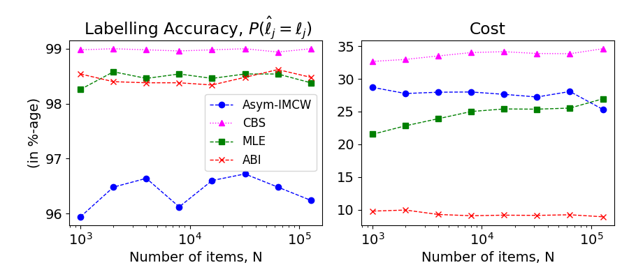
Figure 1: Comparing proposed algorithms (P1-Asym)

Due to space constraints, we present only the results corresponding to the instance P1-Asym here; the results corresponding to P1-Sym along with additional comparisons between Asym-IMCW and Sym-IMCW, can be found in Appendix B. The observations are illustrated in Figure 1. Here, CBS stands for a variant of Asym-IMCW, where the Chernoff stopping rule is replaced by one based on confidence bounds (details in Appendix F).

$\bullet$ We note that Asym-IMCW does meet the prescribed labelling accuracy. Moreover, the Chernoff stopping rule used in Asym-IMCW outperforms the confidence bounds based stopping criterion from a cost standpoint; the latter approach tends to acquire far more label predictions than needed (this also makes its label assignments more accurate, almost $99\%$ accurate, as compared to the prescribed threshold of $95\%$).

$\bullet$ Interestingly, both heuristics (ABI and the MLE based approach) outperform Asym-IMCW, providing a higher labelling accuracy at a lower or comparable cost. As noted before, this is due to their use of the confusion matrix estimates from the explore phase. This motivates the design of alternative approaches, that perform the tasks of confusion matrix estimation and cost-optimal label assignment jointly–a promising avenue for future work (we remark on this further in Section VI).

VI Concluding Remarks

We model the problem of a requester seeking to perform unsupervised binary classification on a multi-class crowdsourcing platform. The requester seeks to minimize the cost of performing this task, subject to an accuracy constraint. Our proposed algorithms combine flavours of fixed budget as well as fixed confidence MAB algorithms.

The reason we do not use a single-shot MAB style algorithm that combines exploration and exploitation is that the confidence intervals on the confusion matrices (using the spectral machinery developed by Anandkumar et al. (2015) and Zhang et al. (2016)) are very loose. Example: a confidence interval of width $\epsilon=0.1$ is available with probability $\geq 0.9$ only when $N$ exceeds  $3\times 10^{33}$ for the instance we consider in our case study. A UCB-style algorithm that uses such confidence intervals would therefore perform very poorly in practice. It is therefore a challenging avenue for future work, to combine the exploration and exploitation aspects of our problem formulation into an algorithm that performs well in practice, and also admits an analytical performance guarantee.

Appendix A Asymmetric Confusion Matrices

In this section, we consider the general case, where the probability that each worker correctly labels an item can depend on the item’s true label. This corresponds to working with asymmetric confusion matrices for each worker class. In this setting, we use the spectral tensor methods developed by [11, 12] to estimate the confusion matrix corresponding to each worker class.

Our algorithm for asymmetric confusion matrices, referred to as Asym-IMCW, is presented as Algorithm 4. Asym-IMCW is structurally similar to Sym-IMCW; it also proceeds in two phases—an explore phase for estimating the confusion matrices and thus identifying the optimal worker class with high probability, and an exploit phase (identical to that in Sym-IMCW) for estimating the true item labels with the prescribed accuracy guarantee using label predictions from the estimated optimal worker class.

Next, we provide a brief description of the explore phase of Asym-IMCW. (The exploit phase of Asym-IMCW is identical to that of Sym-IMCW.)

A-A Explore Phase of Asym-IMCW

The explore phase of Asym-IMCW is based on Algorithm 1 of [12]. Similar to Sym-IMCW, we first obtain a single label prediction for each of the given $N$ items, from all worker classes. Algorithm 1 of [12] then partitions the worker classes into three disjoint groups (say $a,b,$and $c$) and estimates group aggregated confusion matrices (up to a column permutation) for all the three groups. This is done by deploying the robust tensor power method developed by [11] thrice, each time with a different order of $(a,b,c)$. The correct permutation of the columns is determined by the assumption $c_{k}(0),c_{k}(1)>\frac{1}{2}.$ Later, a plug-in estimator for each worker class is used to extract its estimated confusion matrix from that of its group.

For the confusion matrix estimators used in Asym-IMCW, Theorem 3 of [12] establishes PAC guarantees, which states that the estimates are $\epsilon$-accurate with probability at least $1-\delta,$ for large enough $N,$ where the permissible tuples of $\epsilon,$ $\delta,$ and the threshold on $N$ are constrained in terms of the problem parameters. Note that we do not need  $\epsilon$ and $\delta$ to be algorithm computable, and use them only to establish our guarantees in Theorem A.1. For the sake of convenience, we parameterize these in terms of two floating parameters $\gamma_{a},\gamma_{b}\in(0,1)$ satisfying $\gamma_{a}+2\gamma_{b}\leq 1,$ as shown in the proof of Theorem A.1

Algorithm 4 Asymmetric - IMCW

1:Input: prices $\{p_{k}:k\in[M]\}$; error threshold $\alpha$; number of items $N$; items $\{j:j\in[N]\}$;

2:$\cdots\cdots\cdots\cdots\cdots\cdots\cdots\cdots\cdots\cdots$ $\triangleright$ Explore Phase

3:for $j=1,\dots,N$ do

4:     for all $k\in[M]$ do

5:         Collect label prediction on item $j$ at price $p_{k}$      

6:Run Algorithm 1 of [12] and obtain $\hat{c}_{k}(0)$ and $\hat{c}_{k}(1)$ $\forall\ k\in[M]$

7:$\hat{c}_{\hat{k}}(0)\leftarrow\max\{\hat{c}_{\hat{k}}(0),\frac{1}{2}\}$;  $\hat{c}_{\hat{k}}(1)\leftarrow\max\{\hat{c}_{\hat{k}}(1),\frac{1}{2}\}$

8:Set $\hat{k}=\arg\!\min_{k\in[M]}\max\{\frac{p_{k}}{d(\hat{c}_{\hat{k}}(0),0.5)},\frac{p_{k}}{d(\hat{c}_{\hat{k}}(1),0.5)}\}$

9:$\cdots\cdots\cdots\cdots\cdots\cdots\cdots\cdots\cdots\cdots$ $\triangleright$ Exploit Phase

10:for all $j\in[N]$  do

11:     Assign the final label, $\hat{\ell}_{j}=$ DirectionTest($\hat{k}$, $j$, $\alpha$)

A-B Performance Guarantee

We now state our formal performance guarantee for Asym-IMCW.

Theorem A.1

Under the Asym-IMCW algorithm, for each item $j\in[N],$ $P\left(\hat{\ell}_{j}\neq\ell_{j}\right)<\alpha.$ Moreover, for $\gamma_{a},\gamma_{b}\in(0,1),$ that satisfy $\gamma_{a}+2\gamma_{b}\leq 1,$ if $N\geq N_{0}(\gamma_{a},\gamma_{b}),$ where $N_{0}(\gamma_{a},\gamma_{b})$ is an instance dependent constant, then

$$P\left(\hat{k}\neq k^{*}\right)\leq(48+M)\exp\left(1-N^{\gamma_{a}}\right)$$

Finally, denoting the number of label predictions acquired for item $j$ in the exploit phase by $\tau_{\hat{k}},$

$$P\left(\limsup_{\alpha\downarrow 0}\frac{\tau_{\hat{k}}}{\log(1/\alpha)}\leq\frac{1}{d(c_{\hat{k}}(\ell_{j}),0.5)}\right)=1.$$

The exact expression for $N_{0}(\gamma_{a},\gamma_{b})$ is provided in Appendix  D, which also contains the proof of Theorem A.1.

Appendix B Case Study

For a representative case study, we wanted to consider a realistic scenario with different worker classes each represented by a unique confusion matrix. We used the dataset provided by [31] on the Recognizing Textual Entailment (RTE) task (originally proposed by [32]), which had over 8000 labels assigned by 164 unique workers on 108 different items. Post calculating the confusion matrix for each worker, we found that we can choose the following 5 confusion matrices to represent distinct worker classes. Each confusion matrix below is well differentiated from the others to represent a unique class of workers with similar backgrounds and accuracy.

$$C_{1}=\begin{bmatrix}0.94&0.1\\ 0.06&0.90\end{bmatrix}\quad C_{2}=\begin{bmatrix}0.77&0.13\\ 0.23&0.87\end{bmatrix}$$

$$C_{3}=\begin{bmatrix}0.92&0.24\\ 0.08&0.76\end{bmatrix}\quad C_{4}=\begin{bmatrix}0.88&0.18\\ 0.12&0.88\end{bmatrix}$$

$$C_{5}=\begin{bmatrix}0.64&0.34\\ 0.36&0.66\end{bmatrix}$$

These confusion matrices are unknown to our algorithms and are used only to mimic the response from real world workers on any item $j$. In all our experiments, we have set $\alpha=0.05,$ and work with the same $5$ worker classes for accurate comparison.

The pricing model P1 ensures that a label from these worker classes is appropriately priced with decreasing marginal utility across worker classes.

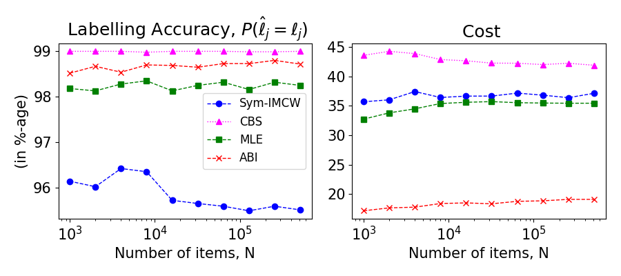
Figure 2: Comparing proposed algorithms on P1-Sym

• Sym-IMCW performs in a similar fashion as Asym-IMCW qualitatively as seen in Figure 2. The prescribed labelling accuracy of atleast 95% is met. Sym-IMCW outperforms the CBS heuristic on the cost front, while the other heuristics, ABI and MLE based approaches, provide better accuracy at lower or comparable costs.

• We compare our algorithms Sym-IMCW and Asym-IMCW by running them on the same instance P1-Sym. The most interesting comparison of Asym-IMCW and Sym-IMCW is in their ability to accurately identify the optimal worker class, $k^{*}$. Figure 3 shows the accuracy in identifying worker classes for Asym-IMCW on both instances and Sym-IMCW on P1-Sym. Sym-IMCW clearly outperforms Asym-IMCW here with the latter catching up as number of items increases. This can be attributed to the more complex machinery in [12] for the estimation of asymmetric confusion matrices, as compared to the symmetric one-coin model.

• The labelling and cost performance of Asym-IMCW on the P1-Sym instance is represented in Figure 4. Asym-IMCW performs very similar to Sym-IMCW on both the labelling and cost standpoint even for smaller number of items. This is likely due to the small $\Delta_{min}$ in the instance considered here (see Table I), so that Asym-IMCW incurs a comparable cost in spite of choosing a (slightly) sub-optimal worker class.

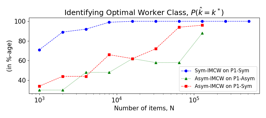
Figure 3: Comparing Asym-IMCW and Sym-IMCW on identification of $k^{*}$

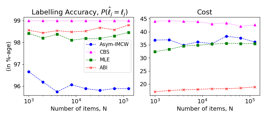
Figure 4: Performance of Asym-IMCW on P1-Sym

Appendix C Proofs for Symmetric Case

C-A Proof of Lemma II.1

We structure this problem as a Two-armed bandit with the reward of the first arm $\mu_{1}$ being either $\mathrm{Bernoulli}(c_{k}(1))$ or $\mathrm{Bernoulli}(1-c_{k}(0))$ depending on $\ell_{j}$. We denote it as $\mathrm{Bernoulli}(c_{k}(\ell_{j},1))$. The second arm is taken as deterministic with $\mu_{2}=\frac{1}{2}$. We thus apply the MAB machinery to decide whether $\mu_{1}>\frac{1}{2}$ or $\mu_{1}<\frac{1}{2}$ and consequently the estimate the true label.
Theorem 6 of [28] guarantees that for an identifiable class $\mathcal{M}$ of two-armed bandits and $\nu=(\nu_{1},\nu_{2})\in\mathcal{M}$ be such that $\mu_{1}\geq\mu_{2}$, any algorithm that is $\alpha-$PAC on $\mathcal{M}$ satisfies

$$\mathbb{E}\left[\tau\right]\geq\frac{1}{c_{*}(\nu)}\log\left(\frac{1}{2.4\alpha}\right),$$

where

$$c_{*}(\nu):=\inf_{(\nu^{{}^{\prime}}_{1},\nu^{{}^{\prime}}_{2})\in\mathcal{M}:\mu^{{}^{\prime}}_{1}\leq\mu^{{}^{\prime}}_{2}}\max\{d(\mu_{1},\mu^{{}^{\prime}}_{1}),d(\mu_{2},\mu^{{}^{\prime}}_{2})\}$$

In our case, since the second arm is deterministic, the class of bandits, $\mathcal{M}$ is quite restricted and $\mu_{2}=\frac{1}{2}$ is constant. Hence, the only choice for $\mu^{{}^{\prime}}_{1}$ in $c_{*}(\nu)$ is $\mu^{{}^{\prime}}_{1}=\frac{1}{2}$ which changes the optimal arm. Hence, for our case, $c_{*}(\nu)=d(\mu_{1},\frac{1}{2})=d(c_{k}(\ell_{j},1),0.5)=d(c_{k}{\ell_{j}},0.5)$ since $d(x,0.5)=d(1-x,0.5)$

C-B Proof of Lemma III.1

Our complete proof for Lemma III.1 is described as follows. We structure this problem as a Two-armed bandit with the reward of the first arm $\mu_{1}$ being either $\mathrm{Bernoulli}(c_{k}(1))$ or $\mathrm{Bernoulli}(1-c_{k}(0))$ depending on $\ell_{j}$. We denote it as $\mathrm{Bernoulli}(c)$, with $c=c_{k}(\ell_{j})$ taking the required value. The second arm is taken as deterministic with $\mu_{2}=\frac{1}{2}$. We thus apply the MAB machinery to decide whether $\mu_{1}>\frac{1}{2}$ or $\mu_{1}<\frac{1}{2}$ and consequently the estimate $\hat{\ell}_{j}$.
Theorem 10 of [30] guarantees that for any sampling strategy, the Chernoff stopping rule with threshold

$$\beta(t,\alpha)=\log\left(\frac{2t}{\alpha}\right)$$

, ensures that the better of the two arms is selected at the end with probability $\geq 1-\alpha$.
For the second part, we use Proposition 13 of [30]. For our set of arms, $w^{*}_{1}=1$ and $w^{*}_{2}=0$. Consequently we only sample the first arm , ensuring $N_{1}(t)=t$ which satisfies all the conditions of Proposition 13 that guarantees for all $\alpha\in(0,1)$,

$$P_{\mathbf{C}_{k}}\left(\limsup_{\alpha\rightarrow 0}\frac{\tau_{k}(\ell_{j})}{\log(1/\alpha)}\leq\frac{1}{d(c_{k}(\ell_{j}),0.5)}\right)=1$$

In other words, the stopping time algorithm achieves the information theoretical lower bound almost surely as $\alpha$ goes down to 0

C-C Proof of Theorem III.1

The performance guarantee in Theorem III.1 is stated in terms of following instance-dependent constants:

$$K_{1} =\left(\frac{18}{\bar{\kappa}\kappa^{3}_{3}}\right)^{1/\gamma}$$

$$K_{2} =\left(\frac{18}{\kappa^{3}_{3}\left(c_{k^{*}}-\frac{\log 2-W_{k^{*}}}{\log(1/(\log 2-W_{k^{*}}))}\right)}\right)^{1/\gamma}$$

$$K_{3} =\max_{k\in[M]\setminus k^{*}}\left(\frac{18}{\kappa^{3}_{3}\left(\frac{\log 2-W_{k}}{2\log(6/(\log 2-W_{k}))}-c_{k}\right)}\right)^{1/\gamma}$$

Here, $\gamma$ is a scalar in $(0,1/2),$ $\bar{\kappa}=\frac{1}{M}\sum^{M}_{k=1}(c_{k}-0.5),$ $\kappa_{3}$ is the third largest element in $\{c_{k}-0.5\}^{M}_{k=1},$ and

$$W^{-1}_{k} =\frac{1}{d(c_{k},0.5)}-\frac{\Delta_{k}}{2p_{k}}\quad\text{ for }k\in[M]\setminus\{k^{*}\},$$

$$W^{-1}_{k^{*}} =\frac{1}{d(c_{k^{*}},0.5)}+\frac{\Delta_{min}}{2p_{k^{*}}}.$$

Finally, with $N_{0}(\gamma)=\max(K_{1},K_{2},K_{3})$ and $N\geq N_{0}(\gamma)$ as in the statement of Theorem III.1, our complete proof is described below.

Proof:

Running steps (1)-(2) of Algorithm 2 of [12] with $N$ items, returns the estimates $\{\hat{c}_{k}\}^{M}_{k=1}$. Using Lemma C.1 with $N\geq\left(\frac{18}{\bar{\kappa}\kappa^{3}_{3}}\right)^{1/\gamma}$, we obtain

$$\max_{k\in[M]}\{\|\hat{c}_{k}-c_{k}\|\}\leq\frac{18}{\kappa^{3}_{3}N^{\gamma}}~{}$$

w.p $\geq 1-M^{2}\exp\left(-\frac{N^{1-2\gamma}}{2}\right).$ Let $G_{k}:=\{|\hat{c}_{k}-c_{k}|<\epsilon\}$ and let $G=\bigcap G_{k}$. Observe that under the event $G_{k}$, for any $\epsilon,\delta>0$, it is true that

$$\frac{1}{d(c_{k}+\epsilon,0.5)}\leq\frac{1}{d(\hat{c}_{k},0.5)}\leq\frac{1}{d(c_{k}-\epsilon,0.5)}$$

Setting $\epsilon=\frac{18}{\kappa^{3}_{3}N^{\gamma}}$ and $\delta=M^{2}\exp\left(-\frac{N^{1-2\gamma}}{2}\right)$, we can prove the theorem as follows

$$P\left(\hat{k}\neq k^{*}\right)$$

$$=P\left(\frac{p_{k^{*}}}{d(\hat{c}_{k^{*}},0.5)}>\min_{k\in[M]\setminus\{k^{*}\}}\frac{p_{k}}{d(\hat{c}_{k},0.5)}\right)$$

$$=P\left(\bigcup_{k\in[M]\setminus k^{*}}\frac{p_{k^{*}}}{d(\hat{c}_{k^{*}},0.5)}>\frac{p_{k}}{d(\hat{c}_{k},0.5)}\right)$$

$$\leq P\left(G\right)P\left(\bigcup_{k\in[M]\setminus k^{*}}\frac{p_{k^{*}}}{d(\hat{c}_{k^{*}},0.5)}>\frac{p_{k}}{d(\hat{c}_{k},0.5)}\mid G\right)+P\left(G^{C}\right)$$

$$<P\left(\bigcup_{k\in[M]\setminus k^{*}}\frac{p_{k^{*}}}{d(c_{k^{*}}-\epsilon,0.5)}>\frac{p_{k}}{d(c_{k}+\epsilon,0.5)}\right)+\delta$$

$$=P\left(\bigcup_{k\in[M]\setminus k^{*}}\frac{p_{k^{*}}}{d(c_{k^{*}}-\epsilon,0.5)}-\frac{p_{k^{*}}}{d(c_{k^{*}},0.5)}>\frac{p_{k}}{d(c_{k}+\epsilon,0.5)}-\frac{p_{k}}{d(c_{k},0.5)}+\Delta_{k}\right)+\delta$$

$$\leq P\left(\frac{p_{k^{*}}}{d(c_{k^{*}}-\epsilon,0.5)}-\frac{p_{k^{*}}}{d(c_{k^{*}},0.5)}>\Delta_{min}/2\right)+P\left(\bigcup_{k\in[M]\setminus k^{*}}\frac{p_{k}}{d(c_{k},0.5)}-\frac{p_{k}}{d(c_{k}+\epsilon,0.5)}>\Delta_{k}/2\right)+\delta$$ (5)

The additional requirement on $N$ gives us

1. For $k=k^{*}$

   $$N\geq\left(\frac{\kappa^{3}_{3}\left(c_{k}-\frac{\log 2-W_{k}}{\log(1/(\log 2-W_{k}))}\right)}{18}\right)^{-1/\gamma}$$

   $$\implies c_{k}-\epsilon\geq\frac{\log 2-W_{k}}{\log(1/(\log 2-W_{k}))}$$

   $$\geq H^{-1}(\log 2-W_{k})$$

   $$\implies H(c_{k}-\epsilon)\leq\log 2-W_{k}~{}\text{(Lemma \ref{lemma:bef})}$$

   $$\implies d(c_{k}-\epsilon,0.5)\geq W_{k}$$

   $$\implies\frac{p_{k}}{d(c_{k}-\epsilon,0.5)}-\frac{p_{k}}{d(c_{k},0.5)}\leq\Delta_{min}/2$$ (6)

2. $\forall k\in[M]\setminus k^{*}$,

   $$N\geq\left(\frac{\kappa^{3}_{3}\left(\frac{\log 2-W_{k}}{2\log(6/(\log 2-W_{k}))}-c_{k}\right)}{18}\right)^{-1/\gamma}$$

   $$\implies c_{k}+\epsilon\leq\frac{\log 2-W_{k}}{2\log(6/(\log 2-W_{k}))}$$

   $$\leq H^{-1}(\log 2-W_{k})$$

   $$\implies H(c_{k}+\epsilon)\geq\log 2-W_{k}$$

   $$\implies d(c_{k}+\epsilon,0.5)\leq W_{k}~{}\text{(Lemma \ref{lemma:bef})}$$

   $$\implies\frac{p_{k}}{d(c_{k},0.5)}-\frac{p_{k}}{d(c_{k}+\epsilon,0.5)}\leq\Delta_{k}/2$$ (7)

Equation (6) and (7) ensure that the first term in Equation (5) is a zero probability event with the given lower bound on $N$ . And thus we can complete Equation (5) as $P\left(\hat{k}\neq k^{*}\right)<\delta$ to complete the proof for the theorem

The proof of the Exploit Stage is provided in Lemma III.1

∎

Lemma C.1

Given $M$ available prices {$p_{k}$ : $k\in[M]$ } with unknown $2\times 2$ symmetric confusion matrices $C_{k}$ for $k\in[M]$, $L$ different items drawn from a $2$-class distribution and $\rho$ such that $\kappa_{3}\geq\rho$, where $\kappa_{3}$ is the third largest element in $\{\mid c_{k}-0.5\mid\}^{M}_{k=1}$, then for any scalar $0<\gamma<0.5$ , if the number of items, $L$, satisfies,

$$L\geq\left(\frac{18}{\bar{\kappa}\rho^{3}}\right)^{1/\gamma}$$

,where $\bar{\kappa}=\frac{1}{M}\sum^{M}_{k=1}(c_{k}-0.5)$ , then the estimates of the confusion matrices returned by Steps(1)-(2) of Algorithm 2 of [12] are bounded as

$$\max_{k\in[M]}\{\|\hat{c}_{k}-c_{k}\|\}\leq\frac{18}{\rho^{3}L^{\gamma}}$$

with probability $\geq 1-M^{2}\exp(-\frac{L^{1-2\gamma}}{2})$

Proof:

The Lemma 13 of [12] says that for any scalar, $0<t<\frac{\bar{\kappa}\kappa^{3}_{3}}{18}$,

$$\max_{k\in[M]}\{\|\hat{c}_{k}-c_{k}\|\}\leq\frac{18t}{\kappa^{3}_{3}}$$

w.p $\geq 1-M^{2}\exp\left(-\frac{Lt^{2}}{2}\right)$
Now set $t=\frac{1}{L^{\gamma}}$, we get

$$\max_{k\in[M]}\{\|\hat{c}_{k}-c_{k}\|\}\leq\frac{18L^{-\gamma}}{\kappa^{3}_{3}}\leq\frac{18}{\rho^{3}L^{\gamma}}$$

w.p $>1-M^{2}\exp\left(-\frac{L^{1-2\gamma}}{2}\right)$ ∎

Lemma C.2

For any $x>0.5$,

$$d(0.5,x)\geq y\iff x\geq\frac{1+\sqrt{1-e^{-2y}}}{2}$$

Proof:

Observe that,

$$d(0.5,x)=\frac{-\log(4x(1-x)}{2}>y$$

, thus we can say

$$4x(1-x) \leq e^{-2y}$$

$$4x^{2}-4x+e^{-2y} \geq 0$$

$$x \geq\frac{1+\sqrt{1-e^{-2y}}}{2}$$

∎

Lemma C.3

The binary entropy function , $H(x)=-x\log(x)-(1-x)\log(1-x)$ satisfies the following

$$\frac{x}{2\log(\frac{6}{x})}\leq H^{-1}(x)\leq\frac{x}{\log(\frac{1}{x})}$$

Appendix D Proofs for Asymmetric Case

The guarantee in Theorem A.1 is stated in terms of the following instance-dependent quantities:

$$w_{min} =\min\{w_{0},w_{1}\},\quad\kappa=\min_{k\in[M]}\min_{i\in\{0,1\}}(2c_{k}(i)-1),$$

$$W =diag(w_{0},w_{1}),\quad\sigma_{L}=\min_{a\neq b\in[M]}\|\textbf{C}_{a}W\textbf{C}_{b}^{T}\|,$$

$$K_{1} =\left(\frac{(72\times 31\times 230)^{2}2^{5}}{w_{min}^{2}\sigma_{L}^{13}}\right)^{1/(1-\gamma_{a}-2\gamma_{b})},$$

$$K_{2} =\left(\frac{w_{min}\sigma_{L}}{72\kappa}\right)^{1/\gamma_{b}},$$

$$K_{3} =\left(c_{k^{*}}(m_{k^{*}})-\frac{\log 2-W_{k^{*}}}{\log(1/(\log 2-W_{k^{*}}))}\right)^{-1/\gamma_{b}},$$

$$K_{4} =\max_{k\in[M]\setminus{k^{*}}}\left(\frac{\log 2-W_{k}}{2\log(6/(\log 2-W_{k}))}-c_{k}(m_{k})\right)^{-1/\gamma_{b}}$$

$$K_{5} =\max_{k\in[M]\setminus{k^{*}}}\left|{\frac{c_{k}(0)-c_{k}(1)}{2}}\right|^{-1/\gamma_{b}}.$$

Here $\gamma_{a}$ and $\gamma_{b}$ are scalars in $(0,1)$ that satisfy $\gamma_{a}+2\gamma_{b}\leq 1$, and

$$m_{k} :=\arg\!\min_{i\in\{0,1\}}\{c_{k}(i)\}$$

$$W^{-1}_{k} =\frac{1}{d(c_{k}(m_{k}),0.5)}-\frac{\Delta_{k}}{2p_{k}}~{}\forall k\in[M]\setminus k^{*}$$

$$W^{-1}_{k^{*}} =\frac{1}{d(c_{k^{*}}(m_{k^{*}}),0.5)}+\frac{\Delta_{min}}{2p_{k^{*}}}$$

Finally, with $N_{0}(\gamma_{a},\gamma_{b})=\max(K_{1},K_{2},K_{3},K_{4},K_{5})$ and $N\geq N_{0}(\gamma_{a},\gamma_{b})$ as in the statement of Theorem A.1, our complete proof is described below.

Proof:

Using Lemma D.1 with $N$ items which satisfy its requirements, we obtain

$$\max_{k\in[M]}\|\hat{C}_{k}-C_{k}\|_{\infty}\leq\epsilon=N^{-\gamma_{b}}$$

w.p $\geq 1-(48+M)\exp\left(1-N^{\gamma_{a}}\right)$ Let $G_{k}:=\{\|\hat{C}_{k}-C_{k}\|_{\infty}\leq\epsilon\}$ and let $G=\bigcap G_{k}$. Under the event $G_{k}$ that the estimates are bounded for $2$-class asymmetric confusion matrices. Additionally define, $c^{m}_{k}=\min\{c_{k}(0),c_{k}(1)\}\forall k$ such that

$$\frac{p_{k}}{d(c^{m}_{k},0.5)}=\max\left\{\frac{p_{k}}{d(c_{k}(0),0.5)},\frac{p_{k}}{d(c_{k}(1),0.5)}\right\}$$

Note that introducing the constraint that $\epsilon\leq\left|\frac{c_{k}(0)-c_{k}(1)}{2}\right|\forall k\in[M]\setminus k^{*}$ ensures that

$$\frac{p_{k}}{d(\hat{c}^{m}_{k},0.5)}=\max\{\frac{p_{k}}{d(\hat{c}^{1}_{k},0.5)},\frac{p_{k}}{d(\hat{c}^{2}_{k},0.5)}\}$$

in other words the estimates $\hat{c}_{k}$ will be ordered identical to their true values. Now we can work in a similar manner as Theorem III.1 with

$$\Delta_{k}=\frac{p_{k}}{d(c^{m}_{k},0.5)}-\frac{p_{k^{*}}}{d(c^{m}_{k^{*}},0.5)}\forall k\in[M]\setminus k^{*}$$

Setting $\epsilon$ as above and $\delta=(48+M)\exp\left(1-N^{\gamma_{a}}\right)$, we can prove part (1) of the theorem as follows

$$P\left(\hat{k}\neq k^{*}\right)$$

$$=P\left(\frac{p_{k^{*}}}{d(\hat{c}^{m}_{k^{*}},0.5)}>\min_{k\in[M]\setminus\{k^{*}\}}\frac{p_{k}}{d(\hat{c}^{m}_{k},0.5)}\right)$$

$$<P\left(\bigcup_{k\in[M]\setminus k^{*}}\frac{p_{k^{*}}}{d(c^{m}_{k^{*}}-\epsilon,0.5)}>\frac{p_{k}}{d(c^{m}_{k}+\epsilon,0.5)}\right)+\delta$$

$$=P\left(\bigcup_{k\in[M]\setminus k^{*}}\frac{p_{k^{*}}}{d(c^{m}_{k^{*}}-\epsilon,0.5)}-\frac{p_{k^{*}}}{d(c^{m}_{k^{*}},0.5)}>\frac{p_{k}}{d(c^{m}_{k}+\epsilon,0.5)}-\frac{p_{k}}{d(c^{m}_{k},0.5)}+\Delta_{k}\right)+\delta$$

$$\leq P\left(\frac{p_{k^{*}}}{d(c^{m}_{k^{*}}-\epsilon,0.5)}-\frac{p_{k^{*}}}{d(c^{m}_{k^{*}},0.5)}>\Delta_{min}/2\right)+P\left(\bigcup_{k\in[M]\setminus k^{*}}\frac{p_{k}}{d(c^{m}_{k},0.5)}-\frac{p_{k}}{d(c^{m}_{k}+\epsilon,0.5)}>\Delta_{k}/2\right)+\delta$$ (8)

The additional requirement on $N$ gives us

1. For $k=k^{*}$

   $$N\geq\left(c^{m}_{k}-\frac{\log 2-W_{k}}{\log(1/(\log 2-W_{k}))}\right)^{-1/\gamma_{b}}$$

   $$\implies c^{m}_{k}-\epsilon\geq\frac{\log 2-W_{k}}{\log(1/(\log 2-W_{k}))}$$

   $$\geq H^{-1}(\log 2-W_{k})$$

   $$\implies H(c^{m}_{k}-\epsilon)\leq\log 2-W_{k}~{}\text{(Lemma \ref{lemma:bef})}$$

   $$\implies d(c^{m}_{k}-\epsilon,0.5)\geq W_{k}$$

   $$\implies\frac{p_{k}}{d(c^{m}_{k}-\epsilon,0.5)}-\frac{p_{k}}{d(c^{m}_{k},0.5)}\leq\Delta_{min}/2$$ (9)

2. $\forall k\in[M]\setminus k^{*}$,

   $$N\geq\left(\frac{\log 2-W_{k}}{2\log(6/(\log 2-W_{k}))}-c^{m}_{k}\right)^{-1/\gamma_{b}}$$

   $$\implies c^{m}_{k}+\epsilon\leq\frac{\log 2-W_{k}}{2\log(6/(\log 2-W_{k}))}$$

   $$\leq H^{-1}(\log 2-W_{k})$$

   $$\implies H(c^{m}_{k}+\epsilon)\geq\log 2-W_{k}$$

   $$\implies d(c^{m}_{k}+\epsilon,0.5)\leq W_{k}~{}\text{(Lemma \ref{lemma:bef})}$$

   $$\implies\frac{p_{k}}{d(c^{m}_{k},0.5)}-\frac{p_{k}}{d(c^{m}_{k}+\epsilon,0.5)}\leq\Delta_{k}/2$$ (10)

3. $\forall k\in[M]\setminus k^{*}$,

   $$N\geq\left|\frac{c_{k}(0)-c_{k}(1)}{2}\right|^{-1/\gamma_{b}}$$

   $$\implies\epsilon\leq\left|\frac{c_{k}(0)-c_{k}(1)}{2}\right|$$ (11)

Equations (9), (10) and (11) ensure that the first term in Equation (8) is a zero probability event with the given lower bound on $N$ . Thus we can complete the proof of the Explore stage after Equation 8 as $P\left(\hat{k}\neq k^{*}\right)\leq\delta$.

The proof of the Exploit Stage is provided in Lemma III.1 ∎

Lemma D.1

Given scalars $\gamma_{a},\gamma_{b}>0$ such that $\gamma_{a}+2\gamma_{b}\leq 1$, and $M$ available prices {$p_{i}$ : $i\in[M]$ } with unknown $k\times k$ confusion matrices $C_{i}$ for $i\in[M]$ and $L$ different items drawn from a $k$-class distribution with priors $W=(w_{1},\cdots,w_{k})$ and 1 observed label on each item from each of the available prices, then if the number of items satisfy, $L$

$$L\geq\left(\frac{(72\times 31\times 230)^{2}k^{5}}{w_{min}^{2}\sigma_{L}^{13}}\right)^{1/(1-\gamma_{a}-2\gamma_{b})}\text{, and}L\geq\left(\frac{w_{min}\sigma_{L}}{36k\kappa}\right)^{1/\gamma_{b}}$$

, then the confusion matrices returned by Algorithm 1 of [12] are bounded as

$$\|\hat{C}_{i}-C_{i}\|_{\infty}\leq L^{-\gamma_{b}}~{}~{}\textit{for all }i\in[M]$$

with probability $\geq 1-\delta$ where $delta=(36+6k+M)\exp\left(1-L^{\gamma_{a}}\right)$ and

1. $\sigma_{L}=\min_{i\neq j\in[M]}\|C_{i}WC_{j}^{T}\|$

2. $\kappa=\min_{i\in[M]}\min_{l\in[K]}\min_{c\in[M]\setminus{l}}C_{ill}-C_{ilc}$

Proof:

Setting $\epsilon=L^{-\gamma_{b}}$ and $\delta=(48+M)\exp\left(1-L^{\gamma_{a}}\right)$ in Theorem 3 of [12] and considering that we have 2 classes of items, we get the required lower bound on $L$ as

$$L \geq\frac{(72\times 31\times 230)^{2}2^{5}}{\epsilon^{2}w_{min}^{2}\sigma_{L}^{13}}(1+\log((36+6k+M)/\delta))$$

$$=\frac{(72\times 31\times 230)^{2}2^{5}}{L^{-2\gamma_{b}}w_{min}^{2}\sigma_{L}^{13}}(1+L^{\gamma_{a}}-1)$$

$$=\frac{(72\times 31\times 230)^{2}2^{5}}{w_{min}^{2}\sigma_{L}^{13}}(L^{\gamma_{a}+2\gamma_{b}})$$

$$L \geq\left(\frac{(72\times 31\times 230)^{2}2^{5}}{w_{min}^{2}\sigma_{L}^{13}}\right)^{1/(1-\gamma_{a}-2\gamma_{b})}$$

The requirement on $\epsilon$ in Theorem 3 of [12] is satisfied because

$$L \geq\left(\frac{w_{min}\sigma_{L}}{72\kappa}\right)^{1/\gamma_{b}}$$

$$\epsilon=L^{-\gamma_{b}} \leq\frac{72\kappa}{w_{min}\sigma_{L}}$$

∎

Appendix E The MLE Heuristic

The MLE based heuristic is based on Lemma IV.2. Our proof for Lemma IV.2 is below

Proof:

Let $Z$ denote the vector of $t^{M}_{\alpha}$ observed labels from as many workers. For simplicity of notation, take the number of labels as $n=t^{M}_{\alpha}$ and let $n_{0}$ and $n_{1}$ denote the number of labels that are 0 and 1 respectively. Now we consider the likelihood of $Z$ under $\ell_{j}$, and say that the MLE $\hat{\ell}_{j}=1$ , when

$$P\left(Z\mid\ell_{j}=0\right) >P\left(Z\mid\ell_{j}=1\right)$$

$$\text{or, }(c_{k}(0))^{n_{0}}(1-c_{k}(0))^{n_{1}} >(1-c_{k}(1))^{n_{0}}(c_{k}(1))^{n_{1}}$$

$$\text{or, }\left(\frac{c_{k}(0)}{1-c_{k}(0)}\right)^{n_{0}}(1-c_{k}(0))^{n} >\left(\frac{1-c_{k}(1)}{c_{k}(1)}\right)^{n_{0}}(c_{k}(1))^{n}$$

$$\text{or, }\frac{n_{0}}{n} >\frac{\log\left(\frac{c_{k}(1)}{1-c_{k}(0)}\right)}{\log\left(\frac{c_{k}(0)}{1-c_{k}(1)}\right)+\log\left(\frac{c_{k}(1)}{1-c_{k}(0)}\right)}\eqqcolon\theta_{k}$$ (12)

In other words, if the fraction of workers predicting 0 exceeds $\theta_{k},$ we assign $\hat{\ell}_{j}=0$ as stated in the lemma. In order to bound the error probability observe that by Chernoff bound for binomial random variables, we have

$$P\left(\hat{\ell}_{j}=1\mid\ell_{j}=0\right)\leq P\left(n_{0}\leq n\theta_{k}\mid\ell_{j}=0\right)\leq e^{-nd(\theta_{k},c_{k}(0))}$$

as here $n_{0}\sim Binomial(n,c_{k}(0))$ under $\ell_{j}=0$. Similarly under $\ell_{j}=1$, $n_{0}\sim Binomial(n,1-c_{k}(1))$

$$P\left(\hat{\ell}_{j}=0\mid\ell_{j}=1\right)\leq P\left(n_{0}\geq n\theta_{k}\mid\ell_{j}=1\right)\leq e^{-nd(\theta_{k},1-c_{k}(1))}$$

Finally we show that $d(\theta_{k},c_{k}(0))=d(\theta_{k},1-c_{k}(1))$ and complete our proof of the error bound in Eq (4) (reproduced below).

$$P\left(\hat{\ell}_{j}\neq\ell_{j}\right)\leq e^{-t^{M}_{\alpha}d(\theta_{k},c_{k}(0))}$$

Observe that,

$$d(\theta_{k},c_{k}(0))-d(\theta_{k},1-c_{k}(1))$$

$$=\theta_{k}\log\left(\frac{1-c_{k}(1)}{c_{k}(0)}\right)+(1-\theta_{k})\log\left(\frac{c_{k}(1)}{1-c_{k}(0)}\right)$$

$$=\frac{\log\left(\frac{c_{k}(1)}{1-c_{k}(0)}\right)\log\left(\frac{1-c_{k}(1)}{c_{k}(0)}\right)+\log\left(\frac{c_{k}(0)}{1-c_{k}(1)}\right)\log\left(\frac{c_{k}(1)}{1-c_{k}(0)}\right)}{\log\left(\frac{c_{k}(0)}{1-c_{k}(1)}\right)+\log\left(\frac{c_{k}(1)}{1-c_{k}(0)}\right)}~{}~{}\text{(Substituting $\theta_{k}$ from Eq~{}\eqref{eqn:theta})}$$

$$=0$$

This completes the proof. ∎

Appendix F The CBS Heuristic

In this section, we formally state the Confidence Bound based Stopping criterion (CBS).

CBS is also a stopping time algorithm that uses confidence bounds instead of the Chernoff stopping rule in Algorithm 2. This is motivated by the fact that for any item $j,$

$$\left[\hat{c}-\sqrt{\frac{\log(1/\alpha)}{2t}},~{}~{}\hat{c}+\sqrt{\frac{\log(1/\alpha)}{2t}}\right],$$

where $\hat{c}$ denotes the average prediction (as also defined in Algorithm 2), is a confidence interval on $c_{\hat{k}}(\ell_{j},1),$ that contains this quantity with probability $\geq 1-\alpha$ (this follows from the Hoeffding inequality). After $t$ label predictions are collected from the worker class $\hat{k}$, the CBS algorithm stops if:

$$|\hat{c}-0.5|>\sqrt{\frac{\log(1/\alpha)}{2t}}$$ (13)

When (13) holds, the final label $\hat{\ell}_{j}$ is assigned identical to line 8 of DirectionTest. For this stopping rule, it is easy to see that $P\left(\hat{\ell}_{j}\neq\ell_{j}\right)\leq\alpha.$

References

- [1] E. Saralioglu and O. Gungor, “Use of crowdsourcing in evaluating post-classification accuracy,” European Journal of Remote Sensing, 2019.
- [2] J. Yi, R. Jin, S. Jain, T. Yang, and A. K. Jain, “Semi-crowdsourced clustering: Generalizing crowd labeling by robust distance metric learning,” in Advances in neural information processing systems. Citeseer, 2012, pp. 1772–1780.
- [3] E. Filatova, “Irony and sarcasm: Corpus generation and analysis using crowdsourcing,” in LREC, 2012.
- [4] V. Pérez-Rosas, B. Kleinberg, A. Lefevre, and R. Mihalcea, “Automatic detection of fake news,” 2017.
- [5] J. V. Nickerson, Y. Sakamoto, and L. Yu, “Structures for creativity: The crowdsourcing of design,” 2011.
- [6] S. Zogaj, U. Bretschneider, and J. Leimeister, “Managing crowdsourced software testing: a case study based insight on the challenges of a crowdsourcing intermediary,” Journal of Business Economics, 2014.
- [7] J. C. Chang, S. Amershi, and E. Kamar, “Revolt: Collaborative crowdsourcing for labeling machine learning datasets,” in Proceedings of ACM CHI 2017, 2017.
- [8] G. Abercrombie and D. Hovy, “Putting sarcasm detection into context: The effects of class imbalance and manual labelling on supervised machine classification of Twitter conversations,” in Proceedings of the ACL 2016 Student Research Workshop, 2016.
- [9] S. Sood, J. Antin, and E. Churchill, “Using crowdsourcing to improve profanity detection,” in AAAI Spring Symposium: Wisdom of the Crowd, 2012.
- [10] A. P. Dawid and A. Skene, “Maximum likelihood estimation of observer error‐rates using the em algorithm,” Journal of The Royal Statistical Society Series C-applied Statistics, 1979.
- [11] A. Anandkumar, R. Ge, D. Hsu, S. M. Kakade, and M. Telgarsky, “Tensor decompositions for learning latent variable models,” Journal of Machine Learning Research, vol. 15, no. 80, pp. 2773–2832, 2014.
- [12] Y. Zhang, X. Chen, D. Zhou, and M. I. Jordan, “Spectral methods meet em: A provably optimal algorithm for crowdsourcing,” Journal of Machine Learning Research, 2016.
- [13] V. C. Raykar, S. Yu, L. H. Zhao, G. H. Valadez, C. Florin, L. Bogoni, and L. Moy, “Learning from crowds,” Journal of Machine Learning Research, 2010.
- [14] D. R. Karger, S. Oh, and D. Shah, “Efficient crowdsourcing for multi-class labeling,” in Proceedings of ACM SIGMETRICS, 2013.
- [15] Q. Liu, J. Peng, and A. T. Ihler, “Variational inference for crowdsourcing,” in Advances in Neural Information Processing Systems, 2012.
- [16] D. Zhou, Q. Liu, J. Platt, and C. Meek, “Aggregating ordinal labels from crowds by minimax conditional entropy,” in Proceedings of the 31st International Conference on Machine Learning, ser. Proceedings of Machine Learning Research, 2014.
- [17] A. Khetan and S. Oh, “Achieving budget-optimality with adaptive schemes in crowdsourcing,” in Advances in Neural Information Processing Systems, 2016.
- [18] A. Ghosh, S. Kale, and P. McAfee, “Who moderates the moderators? crowdsourcing abuse detection in user-generated content,” in Proceedings of the 12th ACM Conference on Electronic Commerce, ser. EC ’11, 2011.
- [19] N. Dalvi, A. Dasgupta, R. Kumar, and V. Rastogi, “Aggregating crowdsourced binary ratings,” in Proceedings of the 22nd International Conference on World Wide Web, ser. WWW ’13, 2013.
- [20] S. Balakrishnan, M. J. Wainwright, and B. Yu, “Statistical guarantees for the EM algorithm: From population to sample-based analysis,” The Annals of Statistics, 2017.
- [21] T. Bonald and R. Combes, “A minimax optimal algorithm for crowdsourcing,” in Advances in Neural Information Processing Systems, vol. 30, 2017.
- [22] A. Rangi and M. Franceschetti, “Multi-armed bandit algorithms for crowdsourcing systems with online estimation of workers’ ability,” in AAMAS, 2018.
- [23] D. Hettiachchi, N. V. Berkel, S. Hosio, V. Kostakos, and J. Gonçalves, “Effect of cognitive abilities on crowdsourcing task performance,” in INTERACT, 2019.
- [24] G. Kazai, “In search of quality in crowdsourcing for search engine evaluation,” in Proceedings of the 33rd European Conference on Advances in Information Retrieval, 2011.
- [25] G. Kazai, J. Kamps, and N. Milic-Frayling, “The face of quality in crowdsourcing relevance labels: Demographics, personality and labeling accuracy,” in Proceedings of the 21st ACM International Conference on Information and Knowledge Management, 2012.
- [26] E. Loepp and J. T. Kelly, “Distinction without a difference? an assessment of mturk worker types,” Research & Politics, 2020.
- [27] D. Shah and C. Lee, “Reducing crowdsourcing to graphon estimation, statistically,” in International Conference on Artificial Intelligence and Statistics, 2018.
- [28] E. Kaufmann, O. Cappé, and A. Garivier, “On the complexity of best-arm identification in multi-armed bandit models,” Journal of Machine Learning Research, vol. 17, no. 1, pp. 1–42, 2016. [Online]. Available: http://jmlr.org/papers/v17/kaufman16a.html
- [29] D. Karger, S. Oh, and D. Shah, “Iterative learning for reliable crowdsourcing systems,” in Advances in Neural Information Processing Systems, 2011.
- [30] A. Garivier and E. Kaufmann, “Optimal best arm identification with fixed confidence,” in 29th Annual Conference on Learning Theory, ser. Proceedings of Machine Learning Research, V. Feldman, A. Rakhlin, and O. Shamir, Eds., vol. 49. Columbia University, New York, New York, USA: PMLR, 23–26 Jun 2016, pp. 998–1027.
- [31] R. Snow, B. O’Connor, D. Jurafsky, and A. Ng, “Cheap and Fast – But is it Good? Evaluating non-expert annotations for natural language tasks,” in Proceedings of the 2008 Conference on Empirical Methods in Natural Language Processing, 2008.
- [32] I. Dagan, O. Glickman, and B. Magnini, “The pascal recognising textual entailment challenge,” in Machine Learning Challenges. Evaluating Predictive Uncertainty, Visual Object Classification, and Recognising Tectual Entailment, J. Quiñonero-Candela, I. Dagan, B. Magnini, and F. d’Alché Buc, Eds. Springer Berlin Heidelberg, 2006, pp. 177–190.