$\Gamma$–limit for a sharp interface model related to pattern formation on biomembranes

Abstract

We derive a macroscopic limit for a sharp interface version of a model proposed in [29] to investigate pattern formation due to competition of chemical and mechanical forces in biomembranes. We identify sub– and supercrital parameter regimes and show with the introduction of the autocorrelation function that the ground state energy leads to the isoperimetric problem in the subcritical regime, which is interpreted to not form fine scale patterns.

1 Introduction

We consider the family of nonlocal isoperimetric problems

$$E_{\gamma,\epsilon}[u]:=\int_{\mathbb{T}^{n}}|\nabla u|-\frac{\gamma}{\epsilon^{n+1}}\int_{{\mathbb{R}^{n}}}{\mathcal{K}}(\tfrac{z}{\epsilon})\fint_{\mathbb{T}^{n}}|u(x+z)-u(x)|\ dx\ dz,$$ (1)

where $u\in BV(\mathbb{T}^{n},\{0,1\})$ and where $\mathbb{T}^{n}$, $n\geq 2$, is the $n$–dimensional unit flat torus. Here, $\gamma>0$ is a fixed parameter and ${\mathcal{K}}$ is a radially symmetric with certain integrability conditions. For details, see Section 2. This class of problems appears in mathematical models of complex materials (such as biomembranes, see below), diblock copolymers (see [10, 25]) and cell motility (see [15]). We derive the limit $\epsilon\to 0$ of the family of models $E_{\gamma,\epsilon}$ in the framework of $\Gamma$–convergence.

The family of functionals (1) is a more general sharp interface version of a model proposed in [29] for the investigation of structures which arise due to competing diffusive and mechanical forces. In particular, it is relevant for the modelling of formation of so called lipid rafts in cell membranes. These are complex nanostructures made up of lipids, proteins and cholesterol and are believed to be responsible for many biological phenomena such as transmembrane signaling and cellular homeostasis (see e.g. [26, 30, 40, 43]). A diffuse interface version of (1) was considered in [19] and can be formulated in terms of the order parameter (i.e. concentration of the chemical) $u$ alone. The resulting energy is given by

$${\mathcal{F}}_{q,\epsilon}[u]=\frac{1}{\epsilon}\int_{\Omega}W(u)+(1-q)\epsilon^{2}|\nabla u|^{2}-u^{2}+u(\mathbf{1}-\epsilon^{2}\Delta)^{-1}u\ dx,$$ (2)

where $\Omega$ is a reference domain, $W$ is a double well potential, $\epsilon>0$ and $q<1$. The solution operator $(\mathbf{1}-\epsilon^{2}\Delta)^{-1}$ is subject to Neumann boundary conditions. In [19] it was shown that for sufficiently small $q>0$, the family ${\mathcal{F}}_{q,\epsilon}$ $\Gamma$–converges to a constant multiple of the perimeter functional as $\epsilon\to 0$ in the $L^{2}$–topology for a standard family of double well potentials (quadratic roots and quadratic growth). We comment on the relation between the diffuse and sharp interface model in Section 2 below.

In this article, we compute explicitely the $\Gamma$–limit of the family $E_{\gamma,\epsilon}$ under suitable assumptions on ${\mathcal{K}}$. We identify two parameter regimes (sub– and supercritical) with respect to $\gamma$ and show that the limit problem is the isoperimetric problem (with modified prefactor) in the subcritical regime. In the supercritical regime, we show that minimising sequences of $E_{\gamma,\epsilon}$ always have unbounded perimeter.

Our main observation is that both the perimeter and the non–local term in (1) can be represented in terms of the (symmetrised) autocorrelation function

$$c_{u}(r):=\fint_{\mathbb{S}^{n-1}}\int_{\mathbb{T}^{n}}u(x+rw)\,u(x)\ dx\ dw.$$ (3)

The formulation of the energy in terms of the autocorrelation function (Lemma 4.2) reveals that although the energy $E_{\gamma,\epsilon}$ is not linear in $u$, it is linear in terms of the autocorrelation function. For the proofs of the upper and lower bound we then can use properties of the autocorrelation function, which allows us to treat a large class of kernels.

Related Literature

Different classes of kernels in isoperimetric problems, where the non–local term has the same scaling as the local one, were considered e.g. in [8, 34, 38, 41]. Representing the energy in terms of the autocorrelation function and exploiting its fine properties has been proposed for a similar family of energies in [28]. There, the autocorrelation function was used to derive a second order expansion for the perimeter functional. However, the family of kernels is subject to different conditions and converge monotonically to a measurable function with certain integrability properties, wheras our family of kernels is assumed to form an approximation of the identity. Due to the highly singular nature of the considered kernels near the origin, our techniques require more information about the regularity of the autocorrelation function. This is not needed in [28] by the assumption of monotone convergence of the kernels. For this purpose, we show regularity properties of the autocorrelation function for polytopes, which are able to approximate any shape of finite perimeter (see (26)).

The $\Gamma$–convergence of (1) where ${\mathcal{K}}$ is the solution to the Helmholtz equation with different boundary conditions was considered in [34]. Their techniques are based on PDE arguments and they require the family of kernels to be solutions of the Helmholtz equation, wheras our techniques work for a larger class of kernels and are based on decay estimates. In particular, we recover the $\Gamma$–convergence result and are able to extend it to kernels which are given by ${\mathcal{K}}+(-\Delta)^{\frac{s}{2}}{\mathcal{K}}=\delta_{0}$ for any $1<s\leq 2$ (see the appendix).

The non–local term appearing in (1) is a periodic version of the quantity already considered in the famous work [6] and was further investigated in [17]. There it was shown that the non–local term converges pointwise to a constant multiple of the perimeter functional (under suitable assumptions on the family of kernels). Our main result will deal with $\Gamma$–convergence, which is in general different to pointwise convergence (see e.g. [16, Example 4.4]).

Lastly, non–local isoperimetric problems of the form (1) have also been considered in the mathematical literature in many different models, e.g. sharp interface variants of the Ohta-Kawasaki model where the non–local term is a Coulomb or Riesz type interaction (see [1, 2, 10, 12, 14, 22, 23, 25, 37]). We note that, contrary to our energy, in these models the non–local term does not have the same scaling as the perimeter functional.

Structure of the paper

In Section 2 we present and discuss our main results. We also outline the proofs. In Section 3 we introduce the autocorrelation function and give some of its properties. In Section 4 we reformulate the energy in terms of the autocorrelation function and present the proofs of our main results, namely the compactness and $\Gamma$–convergence of $E_{\gamma,\epsilon}$ (see Theorem 2.1 and Theorem 2.3). In the Appendix we collect some further calculations.

Notation

Throughout this paper, we write $\mathbb{T}^{n}:=\mathbb{R}^{n}/\mathbb{Z}^{n}$ for the $n$ dimensional flat torus. Without distinction in notation, we identify $(0,1)^{n}$–periodic functions in $\mathbb{R}^{n}$ with functions on $\mathbb{T}^{n}$. We denote $|\Omega|$ for the Lebesgue measure of $\Omega$. For $r>0$ and $x\in\mathbb{R}^{n}$ we denote $B_{r}(x):=\{y\in\mathbb{R}^{n}:|x-y|<r\}$ for the ball around $x$ of radius $r$ and the unit sphere by $\mathbb{S}^{n-1}:=\partial B_{1}(0)$. We denote $\omega_{n}$ for the volume of the unit ball in $\mathbb{R}^{n}$ and $\sigma_{n}:=n\omega_{n}$ for its surface area. We write $A\lesssim B$ if there exists a universal constant $C>0$, such that $A\leq CB$. A function $u\in L^{1}(\mathbb{T}^{n})$ is said to be a function of bounded variation if

$$\int_{\mathbb{T}^{n}}|\nabla u|:=\sup\bigg{\{}\int_{\mathbb{T}^{n}}u(x)\,(\nabla\cdot\varphi)(x)\ dx:\varphi\in C^{1}(\mathbb{T}^{n},\mathbb{R}^{n}),\ \|\varphi\|_{L^{\infty}(\mathbb{T}^{n})}\leq 1\bigg{\}}<\infty.$$ (4)

In this case, we write $u\in BV(\mathbb{T}^{n})$. We denote the perimeter functional $P:L^{1}(\mathbb{T}^{n})\longrightarrow[0,\infty]$ by

$$P[u]:=\left\{\begin{array}[]{lcl}\displaystyle{\int_{\mathbb{T}^{n}}|\nabla u|}&&\text{if }u\in BV(\mathbb{T}^{n},\{0,1\}),\\[10.0pt] +\infty&&\text{if }u\in L^{1}(\mathbb{T}^{n})\setminus BV(\mathbb{T}^{n},\{0,1\}).\end{array}\right.$$ (7)

Acknowledgments

D.B. would like to warmly thank M. Mercker, T. Stiehl, J. Fabiszisky, B. Brietzke, C. Tissot and A. Tribuzio for valuable discussions on the topic. This work is funded by Deutsche Forschungsgemeinschaft (DFG, German Research Foundation) under Germany’s Excellence Strategy EXC-2181/1-39090098 (the Heidelberg STRUCTURES Cluster of Excellence).

2 Statement and discussion of the main results

In this section, we give the precise formulation of our setting and main results. Throughout this article, we assume $n\in\mathbb{N}$, $n\geq 2$. Since we are interested in the case of prescribed volume fraction, we introduce the class of admissible functions

$${\mathcal{A}}:=\bigg{\{}u\in BV(\mathbb{T}^{n},\{0,1\}):\int_{\mathbb{T}^{n}}u(x)\ dx\ =\ \theta\bigg{\}}$$ (8)

for some fixed parameter $0<\theta<1$. We also fix the function ${\mathcal{K}}:\mathbb{R}^{n}\longrightarrow\mathbb{R}$ and define ${\mathcal{K}}_{\epsilon}(z):=\frac{1}{\epsilon^{n}}{\mathcal{K}}(\frac{z}{\epsilon})$. We recall the energy functional

$$E_{\gamma,\epsilon}[u]=P[u]-\frac{\gamma}{\epsilon}\int_{\mathbb{R}^{n}}{\mathcal{K}}_{\epsilon}(z)\int_{\mathbb{T}^{n}}|u(x+z)-u(x)|\ dx\ dz$$ (9)

when $u\in{\mathcal{A}}$, and $E_{\gamma,\epsilon}[u]=+\infty$ for all $u\in L^{1}(\mathbb{T}^{n})\setminus{\mathcal{A}}$. The kernel ${\mathcal{K}}$ is subject to the following conditions:

1. ${\mathcal{K}}$ is radial.

2. $|z|\,{\mathcal{K}}(z)\in L^{1}({\mathbb{R}^{n}})$.

3. $\displaystyle\int_{B_{r}(0)^{c}}{\mathcal{K}}(z)\ dz\geq 0$ for all $r>0$.

By a slight abuse of notation we also write ${\mathcal{K}}(z)={\mathcal{K}}(|z|)$. The imposed conditions (H1)–(H3) are different to the conditions imposed on the family of kernels considered in [17] (see also [34, Theorem 1.2]): although our family of kernels arises as $L^{1}$–dilates of ${\mathcal{K}}$, we relax the assumption of the non–negativity of ${\mathcal{K}}_{\epsilon}$ by (H3).

As the quantity $E_{\gamma,\epsilon}$ is the difference of two positive terms with the same scaling, uniform control of the energy of a sequence of shapes in general does not a priori lead to control of the perimeter. However, we identify the critical parameter

$$\gamma_{\rm crit}:=\frac{n\omega_{n}}{2\omega_{n-1}}\bigg{(}\int_{{\mathbb{R}^{n}}}|z|\,{\mathcal{K}}(z)\ dz\bigg{)}^{-1}$$ (10)

such that for $0<\gamma<\gamma_{\rm crit}$ the perimeter is controlled by the energy, while the perimeter is not controled for $\gamma>\gamma_{\rm crit}$.

Theorem 2.1 (Compactness and non–compactness).

Let $n\geq 2$ and suppose that ${\mathcal{K}}$ satisfies (H1) – (H3).

1. Compactness: Let $0\leq\gamma<\gamma_{\rm crit}$. Then for any sequence $u_{\epsilon}\in L^{1}(\mathbb{T}^{n})$ with $\sup_{\epsilon}E_{\gamma,\epsilon}[u_{\epsilon}]<\infty$ there exists $u\in{\mathcal{A}}$ and a subsequence (not relabeled) such that

   $$u_{\epsilon}\xrightarrow{\epsilon\to 0}u \text{in }L^{1}(\mathbb{T}^{n}).$$ (11)

2. Non–compactness: Let $\gamma\geq\gamma_{\rm crit}$. Then there exists a sequence $u_{\epsilon}\in{\mathcal{A}}$ such that $\sup_{\epsilon}E_{\gamma,\epsilon}[u_{\epsilon}]<\infty$, but there is no $u\in{\mathcal{A}}$ such that $u_{\epsilon}\to u$ in $L^{1}(\mathbb{T}^{n})$ for any subsequence.

Theorem 2.1 identifies the subcritical parameter regime $0\leq\gamma<\gamma_{\rm crit}$ and the supercritical parameter regime $\gamma\geq\gamma_{\rm crit}$. We learn that the local term dominates in the subcritical regime, while in the supercritical regime the destabilising effect of the non–local interaction takes over. The failure of compactness is reflected in uniform lower bounds of the energy and the behaviour of minimising sequences:

Corollary 2.2 (Lower bound of the energy).

Let $n\geq 2$ and suppose that ${\mathcal{K}}$ satisfies (H1) – (H3).

1. Let $0\leq\gamma\leq\gamma_{\rm crit}$. Then $E_{\gamma,\epsilon}\geq 0$ for every $\epsilon>0$.

2. Let $\gamma>\gamma_{\rm crit}$. Then there exists a sequence $u_{\epsilon}\in{\mathcal{A}}$ such that

   $$E_{\gamma,\epsilon}[u_{\epsilon}]\xrightarrow{\epsilon\to 0}-\infty.$$ (12)

   Moreover $\displaystyle{\liminf_{\epsilon\to 0}P[u_{\epsilon}]=\infty}$ for any sequence, such that (12) holds.

We note that in the critical case $\gamma=\gamma_{\rm crit}$, the family of energies $E_{\gamma_{\rm crit},\epsilon}$ does not have the compactness property even though it is bounded from below. This is due to the fact that $0\leq E_{\gamma_{\rm crit},\epsilon}[u]\to 0$ for polytopes (see Proposition 4.3 and 4.4), which are able to approximate any shape of finite perimeter (see (26)). In this case, higher order effects play a role and the theory of higher order $\Gamma$–expansions, developed in [3], should be suitable.

As explained in the introduction, we are interested in the limiting behaviour of minimising sequences as $\epsilon\to 0$. We show that our family of non–local energies $\Gamma$–converges to a local energy functional:

Theorem 2.3 ($\Gamma$–convergence).

Let $n\geq 2$ and suppose that ${\mathcal{K}}$ satisfies (H1) – (H3). Let $0\leq\gamma\leq\gamma_{\rm crit}$. Then $E_{\gamma,\epsilon}\stackrel{{\scriptstyle\Gamma}}{{\longrightarrow}}E_{\gamma,0}$ with respect to the $L^{1}$–topology, where

$$E_{\gamma,0}[u]:=\left\{\begin{array}[]{lcl}(1-\frac{\gamma}{\gamma_{\rm crit}})P[u]&&\text{if }u\in{\mathcal{A}},\\[10.0pt] +\infty&&\text{if }u\in L^{1}(\mathbb{T}^{n})\setminus{\mathcal{A}}.\end{array}\right.$$ (15)

In particular, for every $u\in L^{1}(\mathbb{T}^{n})$ we have:

1. Liminf inequality: For every sequence $u_{\epsilon}\in L^{1}(\mathbb{T}^{n})$ such that $u_{\epsilon}\to u$ in $L^{1}(\mathbb{T}^{n})$ we have $E_{\gamma,0}[u]\leq\liminf_{\epsilon\to 0}E_{\gamma,\epsilon}[u_{\epsilon}]$.

2. Limsup inequalty: There is a sequence $u_{\epsilon}\in L^{1}(\mathbb{T}^{n})$ such that $u_{\epsilon}\to u$ in $L^{1}(\mathbb{T}^{n})$ and $\limsup_{\epsilon\to 0}E_{\gamma,\epsilon}[u_{\epsilon}]\leq E_{\gamma,0}[u]$.

Although the non–local term leads to a reduction of the interfacial cost by a factor of $\frac{\gamma}{\gamma_{\rm crit}}$ in the subcritical regime, the limit problem is simply the isoperimetric problem with a suitably modified prefactor. Hence, the unique minimiser (up to translation and rotation) is given by $u=\chi_{\Omega}$, where $\Omega\subset\mathbb{T}^{n}$ is a single ball or the complement of a single ball if

$$\min\{\theta,1-\theta\}<\Big{(}\frac{2}{n}\Big{)}^{\frac{n}{n+1}}\omega_{n}^{-\frac{1}{n-1}},$$ (16)

and by a single laminate otherwise. If equality holds, both ball and laminate are solutions.

Since our admissible class of functions is restricted to functions with values in $\{0,1\}$, both main theorems hold true with respect to the $L^{p}$–topology for any $p\in[1,\infty)$. Furthermore, we note that the main theorems also hold without the assumption of a fixed volume fraction, i.e. for admissible class of functions ${\mathcal{A}}=BV(\mathbb{T}^{n},\{0,1\})$ as can be shown with minor modifications of the proofs.

Strategy of the proofs

In the following we give an overview of the central strategy of the proofs for the theorems, noting that the detailed proofs are given in Section 4.2. Central to our proofs is the formulation of the energy in terms of the symmetrised autocorrelation function (see Lemma 4.2). At this stage, the radial symmetry of the kernel is crucial and the prefactor $\epsilon^{-1}$ of the non–local term ensures that the weight in the reformulation is an approximation of the identity. This implies that the limiting behaviour of the energy only depends on the autocorrelation function near the origin.

The lower bound in Theorem 2.3 follows from sharp estimates of the auto–correlation function. The upper bound requires higher regularity of the autocorrelation function near the origin in order to pass to the limit. For this purpose, we show that the autocorrelation function is a polynomial near the origin for polytopes (see Lemma 3.3). The reformulation of the energy in terms of the autocorrelation function allows for a splitting into behaviour near the origin (which is regular for polytopes as the autocorrelation function is a polynomial) and far from the origin (which is small since the weight is an approximation of the identity). The remainder of the proof of the upper bound follows from approximation with polytopes (see (26)).

Relation to biological model and comparision of sharp and diffuse interface models

As explained in the introduction, the underlying biological model is a diffuse interface model (see (2)). In the Modica–Mortola theory, there is a connection between diffuse and sharp interface energies in the framework of $\Gamma$–convergence, namely (see [11, 36])

$$\int_{\mathbb{T}^{n}}\frac{1}{\epsilon}W(u)+(1-q)\epsilon|\nabla u|^{2}\ dx\stackrel{{\scriptstyle\Gamma}}{{\longrightarrow}}c_{W,q}\int_{\mathbb{T}^{n}}|\nabla u|$$ (17)

as $\epsilon\to 0$, where

$$c_{W,q}=2\sqrt{1-q}\int_{0}^{1}\sqrt{W(s)}\ ds.$$ (18)

Naively, this would suggest to correspondingly replace the diffuse interface term in (2) by its sharp interface counterpart as in (17). In particular, we note that for ${\mathcal{K}}$ being the solution to

$${\mathcal{K}}-\Delta{\mathcal{K}}=\delta_{0} \text{in }{\mathbb{R}^{n}},$$ (19)

${\mathcal{F}}_{q,\epsilon}$ in (2) is a corresponding diffuse interface model of $E_{\gamma,\epsilon}$ as described above. The energy ${\mathcal{F}}_{q,\epsilon}$ has been considered in [19] where it was shown that there exists $\bar{q}>0$, such that ${\mathcal{F}}_{q,\epsilon}$ $\Gamma$–converges to a constant multiple of the perimeter functional. We note that the results of [19] do not contain a characterisation or estimation of $\bar{q}$, nor the constant appearing in their $\Gamma$–limit. This is due to a nonlinear interpolation inequality shown in [9], which has no explicit description of the constants involved (see also [13]). On the other hand our result shows that the critical value $q_{\rm crit}$ of the corresponding sharp interface model (using the relations (17) and (18)) is given by

$$q_{\rm crit}=1-\Big{(}4\gamma_{\rm crit}\int_{0}^{1}\sqrt{W(s)}\ ds\Big{)}^{-2}.$$ (20)

For ${\mathcal{K}}$ as in (19), we can explicitely compute the corresponding critical value of the sharp interface model and it is given by $\gamma_{\rm crit}=1$ (Lemma A.1). However, one cannot equate the parameter $q_{\rm crit}$ with the corresponding critical value $\bar{q}$ in [19]. Indeed, for a suitable doublewell potential with $\|W\|_{L^{\infty}(0,1)}<\frac{1}{16}$ we would get $q_{\rm crit}<0$. This shows, that $\bar{q}=q_{\rm crit}$ cannot hold, since the result of [19] shows that $\bar{q}>0$. This is probably due to the fact that the sharp interface model neglects effects which might occur of properties of the non–linearity (i.e. the double well potential $W$) such as asymmetry, compressibility of the chemical substance, or behaviour at infinity or the roots. In particular, the interpolation inequality used in [19] in order to show $\bar{q}>0$ only works for double well potentials $W$ which have quadratic roots and superquadratic growth (see also [13, Section 3]). The sharp interface model does not contain information about the double well potential $W$ other than the quantity $\int_{0}^{1}\sqrt{W(s)}\ ds$, which is unrelated to the aformentioned properties.

Our main result is similar to that of [19] in that we find two regimes for a parameter related to the relative strength of the non–local interaction (for our energy $\gamma$, in [19] it is $q$), and the limit problem in the subcritical regime is the isoperimetric problem. The interpretation is the same as in [19], namely in the subcritical parameter regime, fine scale pattern formation does not occur in contrast to experimental results (e.g. stripe patterns or hexagonal array of balls, see [42, 27]). We conjecture fine scale patterns to form for the critical value $\gamma=\gamma_{\rm crit}$, which is subject of current research.

Although the reformulation of the non–local part in terms of the autocorre–lation function (see Lemma 4.2) is also valid for the diffuse interface model (2), our methods used for the sharp interface model (9) fail for two main reasons. First, the autocorrelation function lacks useful properties for Sobolev functions $u\in H^{1}(\mathbb{T}^{n})$ such as $c^{\prime}_{u}(0)=0$ in contrast to Proposition 3.2 (iii). Second, the energy is not anymore solely representable by the autocorrelation function due to the non–linearity $W$, i.e. the diffuse interface model is not linear in the space of autocorrelation functions, which our methods heavily rely on.

Remark 2.4 (Domains with arbitrary periodicity).

The choice of the unit flat torus in contrast to flat tori with side length $\ell>0$ is justified by the scaling of the energy with respect to the reference domain. More precisely, let $\mathbb{T}^{n}_{\ell}:=\mathbb{R}^{n}/(\ell\mathbb{Z})^{n}$ and define

$$E_{\gamma,\epsilon}^{(\ell)}[u]:=\int_{\mathbb{T}^{n}_{\ell}}|\nabla u|-\frac{\gamma}{\epsilon^{n+1}}\int_{\mathbb{R}^{n}}{\mathcal{K}}(\tfrac{z}{\epsilon})\int_{\mathbb{T}^{n}_{\ell}}\frac{|u(x+z)-u(x)|}{|\mathbb{T}^{n}_{\ell}|}\ dx\ dz.$$ (21)

Let $u\in BV(\mathbb{T}^{n},\{0,1\})$ and define the rescaled function $u_{\ell}\in BV(\mathbb{T}_{\ell}^{n},\{0,1\})$ via $u_{\ell}(x):=u(\frac{x}{\ell})$. Then it holds

$$E^{(\ell)}_{\gamma,\epsilon}[u_{\ell}]=\ell^{n-1}E_{\gamma,\ell^{-1}\epsilon}[u].$$ (22)

Thus, the limiting behaviour $\epsilon\to 0$ as well as the subsequent analysis can be reduced to the case of the unit flat torus and the citical value $\gamma_{\rm crit}$ is independent of the choice of $\ell$.

3 Autocorrelation function

We introduce the radially symmetrised autocorrelation function.

Definition 3.1 (Autocorrelation function).

Let $u\in L^{1}(\mathbb{T}^{n})$. We define the autocorrelation function $C_{u}:\mathbb{R}^{n}\longrightarrow\mathbb{R}$ by

$$C_{u}(z):=\int_{\mathbb{T}^{n}}u(x+z)\,u(x)\ dx.$$ (23)

We also define its radially symmetrised version $c_{u}:\mathbb{R}_{+}\longrightarrow\mathbb{R}$ by

$$c_{u}(r):=\frac{1}{\sigma_{n}}\int_{\mathbb{S}^{n-1}}C_{u}(rw)\ dw.$$ (24)

Since $C_{u}$ is $(0,1)^{n}$–periodic, we can identify $C_{u}$ with a function on the flat torus $\mathbb{T}^{n}$. Note that $c_{u}$ is generally not periodic.

The autocorrelation function was studied in the whole space setting (see [32, 20]). It is linked to the covariogram of a set $\Omega\subset\mathbb{R}^{n}$ which is defined by

$$g_{\Omega}(x):=|\Omega\cap(\Omega+x)|=\int_{\mathbb{R}^{n}}u(z)\,u(x+z)\ dz, \text{where }u=\chi_{\Omega}.$$ (25)

In [20] it was shown that $g_{\Omega}$ is a Lipschitz function if and only if $\Omega$ is a set of finite perimeter. The author also presents formulas for the perimeter of $\Omega$ in terms of the covariogram, which we will also exploit in this work (adjusted for subsets of the flat torus $\mathbb{T}^{n}$, see also [28]).

The covariogram has also been investigated in the context of convex geometry (see e.g. [35, 39, 4]). In [35] it was shown that under certain smoothness conditions of the boundary of a set, the covariogram of a convex body is a smooth and they also present formulas for the first and second derivatives in this case. Further applications are random sets [20, 5, 31] and micromagnetism [28].

We briefly recall basic properties of the autocorrelation function:

Proposition 3.2.

Let $u\in BV(\mathbb{T}^{n},\{0,1\})$. Then $C_{u}$ and $c_{u}$ are Lipschitz continuous and it holds:

1. $0\leq C_{u}(x)\leq C_{u}(0)=\|u\|_{L^{1}(\mathbb{T}^{n})}\qquad$ for all $x\in\mathbb{T}^{n}$.

2. $0\leq c_{u}(r)\leq c_{u}(0)=\|u\|_{L^{1}(\mathbb{T}^{n})}\qquad$ for all $r>0$.

3. $\displaystyle{\|c_{u}^{\prime}\|_{L^{\infty}(0,\infty)}=-c_{u}^{\prime}(0)=\frac{\omega_{n-1}}{n\omega_{n}}\int_{\mathbb{T}^{n}}|\nabla u|}$.

Proof.

See [28, Proposition 2.3 and Proposition 2.4].∎

For the proof of the upper bound of Theorem 2.3, in order to pass to the limit $\epsilon\to 0$, we need higher regularity than Lipschitz continuity of the autocorrelation function near the origin. However, one cannot expect higher regularity in general since e.g. $c^{\prime\prime}_{\chi_{\Omega}}(0)=+\infty$ when $\Omega$ has a cusp. We will work around this issue by showing that the autocorrelation function of polytopes is a polynomial near the origin, and hence regular. The desired limit for a general shape of finite perimeter will be dealt with via approximation by polytopes, i.e. for every $u\in BV(\mathbb{T}^{n},\{0,1\})$ there exists a sequence of polytopes $\Omega_{k}\subset\mathbb{T}^{n}$ such that (see [18])

$$\|u-\chi_{\Omega_{k}}\|_{L^{1}(\mathbb{T}^{n})}\xrightarrow{k\to\infty}0, |P[\chi_{\Omega_{k}}]-P[u]|\xrightarrow{k\to\infty}0.$$ (26)

The following result is known in the full space setting for convex polytopes for $n=2$ (see [39, 21]), but we were not able to find versions of it for arbitrary polytopes. We note that a closed set $\Omega\subset\mathbb{T}^{n}$ is said to be a polytope, if the restriction of its canonical embedding to $[0,1]^{n}$ is a polytope in $\mathbb{R}^{n}$.

Lemma 3.3 (Autocorrelation function for polytopes).

Let $\Omega\subset\mathbb{T}^{n}$ be a polytope and let $u:=\chi_{\Omega}$. Then there exists $0<R<1$ and $a_{2},\ldots,a_{n}\in\mathbb{R}$ with $a_{2}\geq 0$ such that

$$c_{u}(r)=\|u\|_{L^{1}(\mathbb{T}^{n})}-r\frac{\omega_{n-1}}{n\omega_{n}}\int_{\mathbb{T}^{n}}|\nabla u|+\sum_{j=2}^{n}a_{j}r^{j} \text{for all }0\leq r<R.$$ (27)

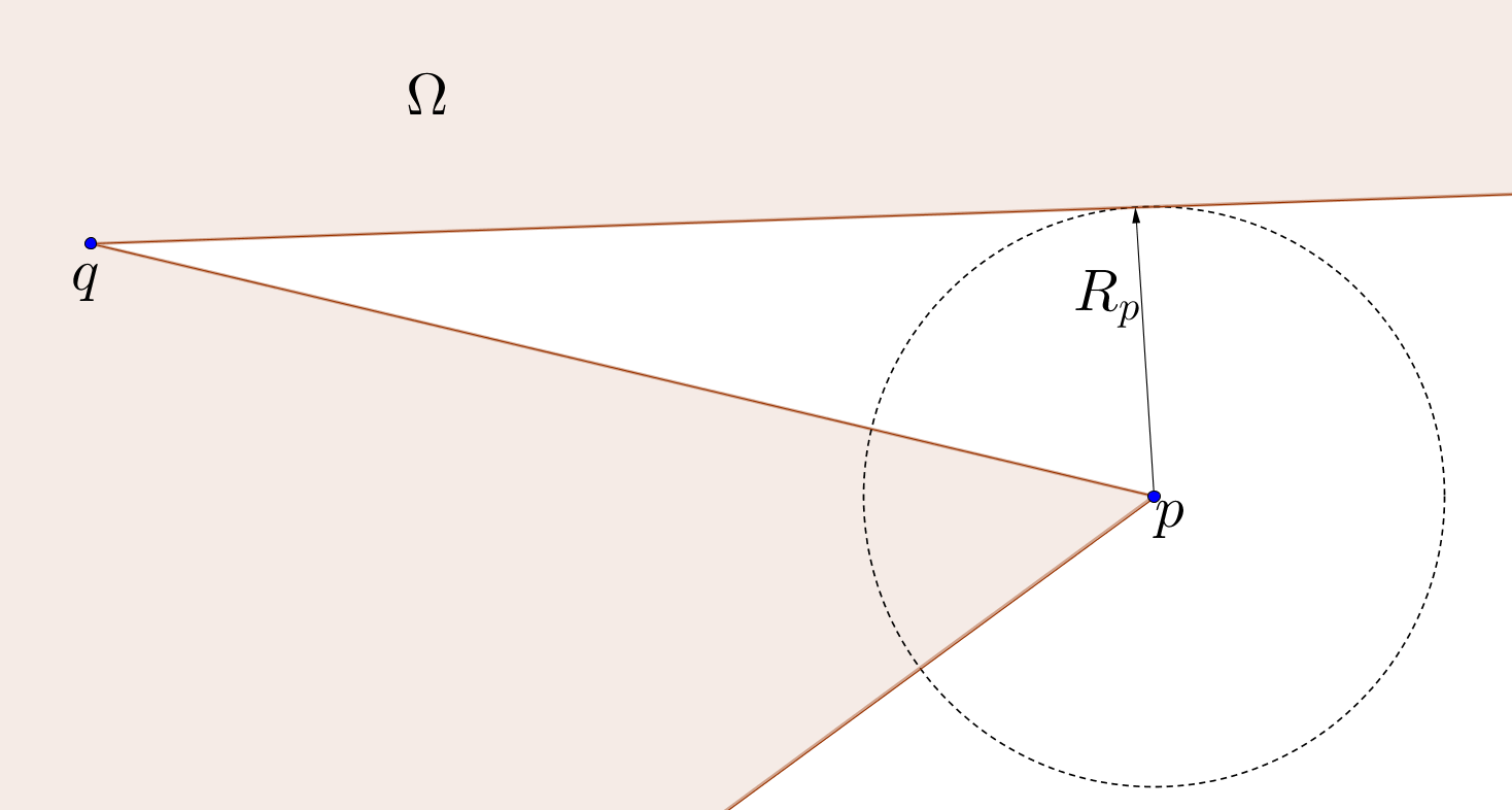
Figure 1: The quantity $R$ ensures that the corners of $\Omega\bigtriangleup\Omega_{rw}$ do not intersect faces which are not adjacent to them.

Proof.

In [28, Lemma 2.5] it was shown that (27) holds for stripes with $a_{2},\ldots,a_{n}=0$. Since the only polytopes which do not have corners are stripes, we can without loss of generality assume that $\Omega$ has at least one corner. We denote the set of corners of $\Omega$ by ${\mathcal{C}}$. We define

$$R:=\frac{1}{2}\min\Big{\{}\min_{p\in{\mathcal{C}}}R_{p},\min_{\begin{subarray}{c}p,q\in{\mathcal{C}}\\ p\neq q\end{subarray}}\operatorname*{dist}(p,q)\Big{\}}>0,$$ (28)

where for any $p\in{\mathcal{C}}$ we set

$$R_{p} :=\sup\big{\{}\varrho>0:\begin{subarray}{c}B_{\varrho}(p)\cap\Omega\text{ and }B_{\varrho}(p)\cap\Omega^{c}\text{ have}\\ \text{only one connected component}\end{subarray}\big{\}}>0.$$ (29)

Let $r>0$, $w\in\mathbb{S}^{n-1}$ and let $\Omega_{rw}:=\Omega+rw$. Then

$$C_{u}(0)-C_{u}(rw)=|\Omega_{rw}\setminus\Omega|=|\Omega\setminus\Omega_{rw}|=\frac{1}{2}|\Omega\bigtriangleup\Omega_{rw}|,$$ (30)

where $\bigtriangleup$ denotes the symmetric difference. Since $C_{u}(0)=\|u\|_{L^{1}(\mathbb{T}^{n})}=|\Omega|$ by Proposition 3.2 (i) it hence remains to calculate $|\Omega\bigtriangleup\Omega_{rw}|$ and its dependence on $r$.

We assume that $w\not\in\SS$, where $\SS\subset\mathbb{S}^{n-1}$ is the negligible set of vectors which are tangential to any of the (finitely many) faces of $\Omega$. By the choice of $R$, the number of faces $N$ of $\Omega\bigtriangleup\Omega_{rw}$ is then is independent of $r\in(0,R)$ and independent of $w$ (see Figure 1). Furthermore, there exist convex trapezoids $T_{rw}^{(1)},\ldots T_{rw}^{(N)}\subset\mathbb{T}^{n}$ with pairwise disjoint interiors such that (see Figure 2)

$$\Omega\bigtriangleup\Omega_{rw}=\bigcup_{i=1}^{N}T_{rw}^{(i)} \text{for all }0<r<R,\ w\in\mathbb{S}^{n-1}\setminus\SS.$$ (31)

Each of these convex trapezoids $T_{rw}^{(i)}$, $i\in\{1,\ldots,N\}$ is determined by a system of linear inequalities

$$T_{rw}^{(i)}=\{x\in\mathbb{T}^{n}:A^{(i)}x\leq b^{(i)},\ A^{(i)}[x+rw]\leq b^{(i)}\},$$ (32)

where for $x,y\in\mathbb{T}^{n}$ we denote $x\leq y$ if and only if $x_{j}\leq y_{j}\!\mod 1$ for every $j\in\{1,\ldots,n\}$ and for some matrices $A^{(i)}\in\mathbb{R}^{2N\times n}$ and vectors $b^{(i)}\in\mathbb{T}^{2N}$. By a slicing argument there exist $d_{1}^{(i)}(w),\ldots,d_{n}^{(i)}(w)\in\mathbb{R}$ such that (see Fig. 3)

$$|T_{rw}^{(i)}|=\sum_{k=1}^{n}d_{k}^{(i)}\!(w)\,r^{k}.$$ (33)

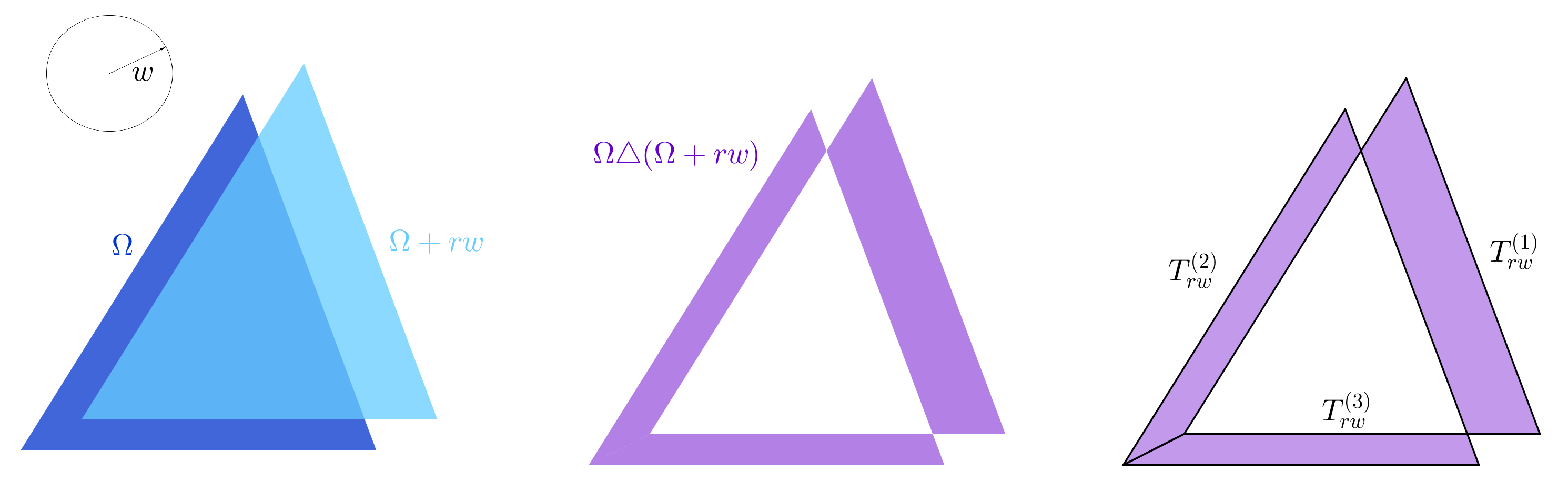
Figure 2: Construction of the trapezoids $T_{rw}^{(i)}$.

More precisely, for $x=(x_{1},x^{\prime})$, there exist at most $2N$ intervals $I_{m_{1}}=[f_{m_{1}}(x^{\prime},rw),g_{m_{1}}(x^{\prime},rw)]$, where $f_{m_{1}}$ and $g_{m_{1}}$ depend in an affine way on $x^{\prime}$ and $rw$, and convex polytopes $K_{m_{1}}\subset\mathbb{T}^{n-1}$ such that

$$|T_{rw}^{i}|=\sum_{m_{1}=1}^{2N}\int_{K_{m_{1}}}\int_{I_{m_{1}}}\ dx_{1}\ dx^{\prime}=\sum_{m_{1}=1}^{2N}\int_{K_{m_{1}}}g_{m_{1}}(x^{\prime},rw)-f_{m_{1}}(x^{\prime},rw)\ dx^{\prime}.$$ (34)

The integrand is now a polynomial in $r$ of degree $1$ and the set of integration is again a convex polytope of the form (32) (reduced in dimension, with different matrices $A^{(i)}$ and $b^{(i)}$). Iteratively, we obtain in the $l$-th step convex polytopes $K_{m_{l}}$ and a polynomial $f_{m_{1},\ldots,m_{l}}$ of degree $l$ such that

$$|T_{rw}^{i}|=\sum_{m_{1}=1}^{2N}\dots\sum_{m_{l}=1}^{2N}\int_{K_{m_{l}}}f_{m_{1},\ldots,m_{l}}(x_{l+1},...,x_{n},rw)\ d(x_{l+1},...,x_{n}).$$ (35)

The algorithm terminates after $n$ steps and leaves a polynomial in $r$ of degree $n$ as described in (33). The assertion now follows from (33) by combining the above identities, i.e.

$$C_{u}(rw)=|\Omega|-\frac{1}{2}\sum_{i=1}^{N}|T_{rw}^{(i)}|\ =\|u\|_{L^{1}(\mathbb{T}^{n})}-\frac{1}{2}\sum_{i=1}^{N}\sum_{k=1}^{n}d_{k}^{(i)}(w)r^{k}$$ (36)

for all $r\in(0,R)$. Averaging with respect to $w$ then yields

$$c_{u}(r)=\|u\|_{L^{1}(\mathbb{T}^{n})}+\sum_{j=1}^{n}a_{j}r^{j} \text{for all }0\leq r<R$$ (37)

for some $a_{1},\ldots,a_{n}\in\mathbb{R}$. Proposition 3.2 (iii) shows that $a_{1}=-\frac{\omega_{n-1}}{n\omega_{n}}P[u]$. By (37) we have $c^{\prime\prime}(0)=2a_{2}$. In view of Proposition 3.2 (iii) we have $c^{\prime\prime}(0)\geq 0$ and hence $a_{2}\geq 0$.

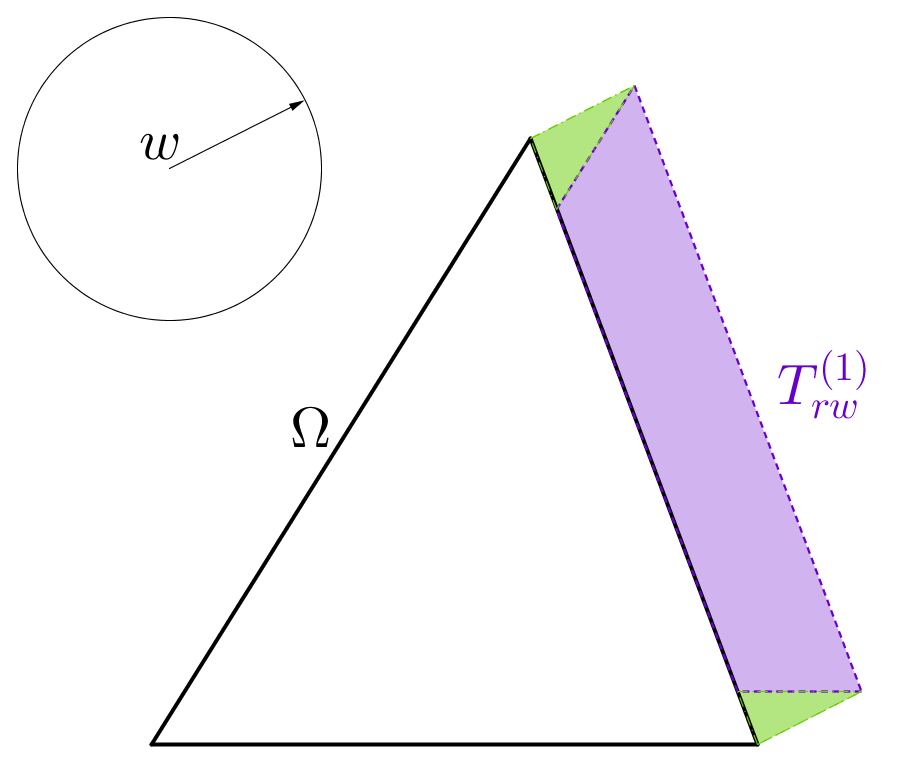
Figure 3: Sketch of the polynomial dependence on $r$ of $|T_{rw}^{(1)}|$. The height of the trapezium is given by $h=r|\nu\cdot w|$, where $\nu$ is the outward normal of the corresponding face. The volume of the green triangles is of order $r^{2}$.

∎

Remark 3.4 (Full space setting).

We note that with analogous arguments the result of Lemma 3.3 also holds in the full space setting.

4 Compactness and $\Gamma$–convergence

4.1 Reformulation of the energy

For the subsequent analysis it is convenient to use the integrated kernel

$$\Phi(r)\ :=\ \sigma_{n}\int_{r}^{\infty}\rho^{n-1}{\mathcal{K}}(\rho)\ d\rho\ =\ \int_{B_{r}(0)^{c}}{\mathcal{K}}(z)\ dz \text{for all }r>0,$$ (38)

instead of the kernel itself. We collect some basic properties of $\Phi$ which follow from our assumptions on ${\mathcal{K}}$:

Proposition 4.1 (Basic properties of $\Phi$).

Assume ${\mathcal{K}}$ satisfies (H1) – (H3). Let $\Phi:(0,\infty)\longrightarrow\mathbb{R}$ be given by (38) and let $\Phi_{\epsilon}(r):=\frac{1}{\epsilon}\Phi(\frac{r}{\epsilon})$. Then $\Phi\in L^{1}(0,\infty)$ with $\Phi\geq 0$. Furthermore,

1. $\displaystyle\lim_{r\to\infty}r\Phi(r)=\lim_{r\to 0}r\Phi(r)=0$.

2. $\displaystyle\int_{0}^{\infty}\Phi(r)\ dr=\int_{{\mathbb{R}^{n}}}|z|\,{\mathcal{K}}(z)\ dz<\infty$.

3. $\displaystyle\int_{0}^{1}r^{j}\Phi_{\epsilon}(r)\ dr\xrightarrow{\epsilon\to 0}0$  for $j\geq 1$.

Proof.

By definition of $\Phi$ and (H3) we have $\Phi\geq 0$ and

$$\Phi^{\prime}(r)\ =\ -\sigma_{n}r^{n-1}{\mathcal{K}}(r)\qquad\text{ for all $r>0$}.$$ (39)

By definition of $\Phi$ and assumption (H2) we have

$$|R\Phi(R)|\leq\sigma_{n}R\int_{R}^{\infty}\rho^{n-1}|{\mathcal{K}}(\rho)|\ d\rho\ \stackrel{{\scriptstyle\eqref{def-Phi}}}{{\leq}}\ \sigma_{n}\int_{R}^{\infty}\rho^{n}|{\mathcal{K}}(\rho)|\ d\rho\ \to\ 0$$ (40)

as $R\to\infty$. Moreover, from Fatou’s Lemma we obtain

$$\limsup_{\varrho\to 0}\varrho\Phi(\varrho)\leq\int_{0}^{\infty}\rho^{n-1}|{\mathcal{K}}(\rho)|\bigg{(}\limsup_{\varrho\to 0}\varrho\chi_{(\varrho,\infty)}(\rho)\bigg{)}\ d\rho=0,$$ (41)

which shows that (i) holds. Integrating by parts we get for $0<\varrho<R<\infty$

$$\sigma_{n}\int_{\varrho}^{R}r^{n}{\mathcal{K}}(r)\ dr\ \stackrel{{\scriptstyle\eqref{kernel-properties-derivative}}}{{=}}-\int_{\varrho}^{R}r\Phi^{\prime}(r)\ dr=-r\,\Phi(r)\bigg{|}_{\varrho}^{R}+\int_{\varrho}^{R}\Phi(r)\ dr,$$ (42)

which yields (ii) in the limits $\varrho\to 0$ and $R\to\infty$ by (i) and the Dominated Convergence Theorem. Assertion (iii) holds since $\Phi\in L^{1}(0,\infty)$. ∎

We are ready to rewrite the nonlocal term in $E_{\gamma,\epsilon}$ in terms of the symmetrised autocorrelation function and the integrated kernel $\Phi$:

Lemma 4.2 (Representation of energy by autocorrelation function).

Let $\gamma,\epsilon>0$ and suppose ${\mathcal{K}}$ satisfies (H1)–(H3). Let $\Phi$ be given by (38) and let $\Phi_{\epsilon}(r):=\frac{1}{\epsilon}\Phi(\frac{r}{\epsilon})$. Then

$$E_{\gamma,\epsilon}[u]=2\gamma_{\rm crit}\int_{0}^{\infty}\Phi_{\epsilon}(r)\,\bigg{[}\frac{\gamma}{\gamma_{\rm crit}}c^{\prime}_{u}(r)-c^{\prime}(0)\bigg{]}\ dr \text{for all }u\in{\mathcal{A}},$$ (43)

where $\gamma_{\rm crit}$ is represented in terms of $\Phi$ via

$$\gamma_{\rm crit}\ =\ \frac{n\omega_{n}}{2\omega_{n-1}}\|\Phi\|_{L^{1}(0,\infty)}^{-1}.$$ (44)

Proof.

We first note that the representation (44) follows from Proposition (ii) together with (10). Since $u$ only takes values in $\{0,1\}$ we have with Proposition 3.2 (i)

$$\frac{1}{\epsilon}\int_{\mathbb{R}^{n}}{\mathcal{K}}_{\epsilon}(z) \int_{\mathbb{T}^{n}}|u(x)-u(x+z)|\ dx\ dz$$ (45)

$$=\frac{1}{\epsilon}\int_{\mathbb{R}^{n}}{\mathcal{K}}_{\epsilon}(z)\int_{\mathbb{T}^{n}}|u(x)-u(x+z)|^{2}\ dx\ dz$$ (46)

$$=\frac{2}{\epsilon}\int_{\mathbb{R}^{n}}{\mathcal{K}}_{\epsilon}(z)\bigg{[}\int_{\mathbb{T}^{n}}|u(x)|^{2}\ dx-\int_{\mathbb{T}^{n}}u(x)\,u(x+z)\ dx\bigg{]}\ dz$$ (47)

$$=\frac{2}{\epsilon}\int_{\mathbb{R}^{n}}{\mathcal{K}}_{\epsilon}(z)\,[C_{u}(0)-C_{u}(z)]\ dz$$ (48)

$$=\frac{2\sigma_{n}}{\epsilon^{n+1}}\int_{0}^{\infty}r^{n-1}{\mathcal{K}}(\tfrac{r}{\epsilon})\,[c_{u}(0)-c_{u}(r)]\ dr,$$ (49)

where in the last line we switched to polar coordinates. Let $0<\varrho<R<\infty$. Noting that $c_{u}$ is Lipschitz (Proposition 3.2), we integrate by parts to obtain

$$\frac{2\sigma_{n}}{\epsilon^{n+1}} \int_{\varrho}^{R}r^{n-1}{\mathcal{K}}(\tfrac{r}{\epsilon})\,[c_{u}(0)-c_{u}(r)]\ dr$$ (50)

$$\kern-4.0pt\stackrel{{\scriptstyle\eqref{kernel-properties-derivative}}}{{=}}-\frac{2}{\epsilon}\int_{\varrho}^{R}[\Phi(\tfrac{r}{\epsilon})]^{\prime}\,[c_{u}(0)-c_{u}(r)]\ dr$$ (51)

$$=\ -2\Phi_{\epsilon}(r)\,[c_{u}(0)-c_{u}(r)]\bigg{|}_{\varrho}^{R}-2\int_{\varrho}^{R}\Phi_{\epsilon}(r)\,c^{\prime}_{u}(r)\ dr,$$ (52)

noting that $\Phi_{\epsilon}(r)=\frac{1}{\epsilon}\Phi(\frac{r}{\epsilon})$. Using Proposition 3.2 (iii) we obtain

$$|\Phi_{\epsilon}(r)\,[c_{u}(0)-c_{u}(r)]|\lesssim r\Phi_{\epsilon}(r)\,P[u] \text{for all }r>0.$$ (53)

Thus the boundary terms in (52) vanish in the limit $\varrho\to 0$ and $R\to\infty$ by Proposition 4.1 (i). It follows from the Dominated Convergence Theorem and the computations above that

$$\frac{1}{\epsilon}\int_{\mathbb{R}^{n}}{\mathcal{K}}_{\epsilon}(z)\int_{\mathbb{T}^{n}}|u(x)-u(x+z)|\ dx=-2\int_{0}^{\infty}\Phi_{\epsilon}(r)\,c^{\prime}_{u}(r)\ dr.$$ (54)

The claim follows by inserting (54) into (9) and using Proposition 3.2 (iii) to rewrite $P[u]$ in terms of $c^{\prime}_{u}(0)$. ∎

4.2 Proofs of the main theorems

We next use the reformulation of the energy $E_{\gamma,\epsilon}$ from Lemma 4.2 to show that the limit energy is a pointwise lower bound. This will simplify the proof of the compactness in Theorem 2.1 and the liminf inequality of Theorem 2.3. It relies on the bound $c_{u}^{\prime}(0)=\min_{r\geq 0}c_{u}^{\prime}(r)$ for all $u\in{\mathcal{A}}$ (Prop. 3.2 (iii)).

Proposition 4.3 (Lower bound for the energy).

Let $\gamma,\epsilon>0$ and suppose that ${\mathcal{K}}$ satisfies (H1)–(H3). Then

$$E_{\gamma,0}[u]\leq E_{\gamma,\epsilon}[u] \text{for all }u\in{\mathcal{A}}.$$ (55)

Proof.

By Proposition 4.1 (iii), Proposition 3.2 (iii) and Lemma 4.2 we obtain

$$E_{\gamma,0}[u]\ \stackrel{{\scriptstyle\eqref{gam-Phi}}}{{=}}2\gamma_{\rm crit}\int_{0}^{\infty}\Phi_{\epsilon}(r)\,\bigg{[}\frac{\gamma}{\gamma_{\rm crit}}c^{\prime}_{u}(0)-c_{u}^{\prime}(0)\bigg{]}\ dr$$ (56)

$$\leq\ 2\gamma_{\rm crit}\int_{0}^{\infty}\Phi_{\epsilon}(r)\,\bigg{[}\frac{\gamma}{\gamma_{\rm crit}}c^{\prime}_{u}(r)-c_{u}^{\prime}(0)\bigg{]}\ dr\ =\ E_{\gamma,\epsilon}[u].$$ (57)

∎

The next proposition is a convergence result and simplifies the non–compact-ness (Theorem 2.1 (ii)) and limsup inequality of Theorem 2.3. The key observation is that the family of integral kernels $\|\Phi\|_{L^{1}(\mathbb{R}_{+})}^{-1}\Phi_{\epsilon}$ forms an approximation of the identity, so we formally achieve with the reformulation of the energy (see Lemma 4.2)

$$E_{\gamma,\epsilon}[u] =2\gamma_{\rm crit}\int_{0}^{\infty}\Phi_{\epsilon}(r)\,\bigg{[}\frac{\gamma}{\gamma_{\rm crit}}c^{\prime}_{u}(r)-c^{\prime}(0)\bigg{]}\ dr$$ (58)

$$\xrightarrow{\epsilon\to 0}2\gamma_{\rm crit}\|\Phi\|_{L^{1}(0,\infty)}\,\langle\delta_{0},\tfrac{\gamma}{\gamma_{\rm crit}}c^{\prime}_{u}(r)-c^{\prime}(0)\rangle=E_{\gamma,0}[u].$$ (59)

However, for general functions $u\in{\mathcal{A}}$ it is not clear if the convergence $E_{\gamma,\epsilon}[u]\to E_{\gamma,0}[u]$ holds pointwise since the function $c_{u}^{\prime}$ is not differentiable at the origin in general. We hence consider the smaller class of polytopal domains. This is where we use the formula for the autocorrelation function for polytopes (see Lemma 3.3).

Proposition 4.4 (Pointwise convergence for polytopes).

Let $\gamma>0$ and suppose ${\mathcal{K}}$ satisfies (H1)–(H3). Let $\Omega\subset\mathbb{T}^{n}$ be a polytope and let $u=\chi_{\Omega}$. Then

$$E_{\gamma,\epsilon}[u]\xrightarrow{\epsilon\to 0}E_{\gamma,0}[u].$$ (60)

Proof.

Let $\epsilon>0$. It suffices to show that the non–local term converges, i.e. (see Lemma 4.2 and (54))

$$\int_{0}^{\infty} \Phi_{\epsilon}(r)\,c^{\prime}_{u}(r)\ dr\xrightarrow{\epsilon\to 0}-\frac{1}{2\gamma_{\rm crit}}P[u].$$ (61)

Lemma 3.3 yields the existence of $a_{1},\ldots,a_{n-1}\in\mathbb{R}$ and $0<R<1$ such that

$$c^{\prime}_{u}(r)=-\frac{\omega_{n-1}}{n\omega_{n}}P[u]+\sum_{j=1}^{n-1}a_{j}\,r^{j} \text{for all }0<r<R.$$ (62)

We use this identity to compute

$$\int_{0}^{\infty} \Phi_{\epsilon}(r)\,c^{\prime}_{u}(r)\ dr$$ (63)

$$= -\frac{\omega_{n-1}}{n\omega_{n}}P[u]\int_{0}^{R}\Phi_{\epsilon}(r)\ dr+\sum_{j=1}^{n-1}a_{j}\int_{0}^{R}r^{j}\Phi_{\epsilon}(r)\ dr+\int_{R}^{\infty}\Phi_{\epsilon}(r)\,c^{\prime}_{u}(r)\ dr$$ (64)

$$= -\frac{\omega_{n-1}}{n\omega_{n}}P[u]\,I_{1}^{(\epsilon)}+I_{2}^{(\epsilon)}+I_{3}^{(\epsilon)}.$$ (65)

For the first integral, we observe that by monotone convergence

$$I_{1}^{(\epsilon)} =\int_{0}^{\frac{R}{\epsilon}}\Phi(r)\ dr\xrightarrow{\epsilon\to 0}\|\Phi\|_{L^{1}(0,\infty)}.$$ (66)

For the second integral we use Proposition 4.1 (iii) to obtain

$$|I_{2}^{(\epsilon)}| \leq\sum_{j=1}^{n-1}|a_{j}|\int_{0}^{1}r^{j}\Phi_{\epsilon}(r)\ dr\xrightarrow{\epsilon\to 0}0.$$ (67)

For the third integral, using Proposition 3.2 (iii) we have

$$|I_{3}^{(\epsilon)}| \leq\int_{R}^{\infty}\Phi_{\epsilon}(r)\ |c_{u}^{\prime}(r)|\ dr\leq\frac{\omega_{n-1}}{n\omega_{n}}P[u]\int_{\frac{R}{\epsilon}}^{\infty}\Phi(r)\ dr\xrightarrow{\epsilon\to 0}0.$$ (68)

Altogether (61) follows. ∎

We are now in the position to prove the compactness (Theorem 2.1 (i)) and non–compactness (Theorem 2.1 (ii)) of $E_{\gamma,\epsilon}$:

Proof of Theorem 2.1.

In order to prove assertion (i) we use Proposition 4.3 to obtain

$$0\leq\Big{(}1-\frac{\gamma}{\gamma_{\rm crit}}\Big{)}P[u_{\epsilon}]=E_{\gamma,0}[u_{\epsilon}] \leq E_{\gamma,\epsilon}[u_{\epsilon}]\lesssim 1$$ (69)

uniformly in $\epsilon$. Using the $L^{1}$–compactness of the perimeter functional proves the claim. In order to prove assertion (ii) we construct a sequence of laminates with the desired properties. We define $\Omega:=(0,\theta)\times[0,1)^{n-1}\subset\mathbb{T}^{n}$ and $v_{k}(x):=\chi_{\Omega}(kx)$. Then $P[v_{k}]=2^{k+1}$ and $v_{k}\in{\mathcal{A}}$ for all $k\in\mathbb{N}$. Moreover, there does not exist a subsequence of $v_{k}$ which converges in $L^{1}$. Indeed, assume there exists a subsequence (not relabeled) and $v\in L^{1}(\mathbb{T}^{n},\{0,1\})$, such that $v_{k}\to v$ in $L^{1}$ as $k\to\infty$. Then $\|v\|_{L^{1}(\mathbb{T}^{n})}=\theta$. We note that $v_{k}\rightharpoonup^{*}\theta$ in $L^{\infty}$ as $k\to\infty$ (see [7, Example 2.7]) and thus

$$\|v_{k}-v\|_{L^{1}(\mathbb{T}^{n})} =\int_{\mathbb{T}^{n}}v_{k}(x)\ dx+\int_{\mathbb{T}^{n}}v(x)\ dx-2\int_{\mathbb{T}^{n}}v_{k}(x)\,v(x)\ dx$$ (70)

$$\xrightarrow{k\to\infty}2\theta-2\theta^{2}\neq 0,$$ (71)

a contradiction. Further, from Proposition 4.4 we obtain

$$E_{\gamma,\epsilon}[v_{k}]\xrightarrow{\epsilon\to 0}\Big{(}1-\frac{\gamma}{\gamma_{\rm crit}}\Big{)}P[v_{k}]\leq 0,$$ (72)

since $\gamma\geq\gamma_{\rm crit}$. Hence, for all $k\in\mathbb{N}$ there exists $\epsilon^{*}(k)$ such that

$$|E_{\gamma,\epsilon}[v_{k}]-E_{\gamma,0}[v_{k}]|<\frac{1}{k} \text{for all }0<\epsilon<\epsilon^{*}.$$ (73)

For $\frac{1}{2}\min\{\frac{1}{k+1},\epsilon^{*}(k+1)\}\leq\epsilon\leq\frac{1}{2}\min\{\frac{1}{k},\epsilon^{*}(k)\}$, we choose $u_{\epsilon}=v_{k}$. Then there does not exist an $L^{1}$–convergent subsequence as was shown above, and

$$E_{\gamma,\epsilon}[u_{\epsilon}]\stackrel{{\scriptstyle\eqref{eq:noncompact_approx}}}{{\leq}}E_{\gamma,0}[v_{k}]+\frac{1}{k}\leq 3,$$ (74)

from which the claim follows. ∎

From the techniques used to prove Theorem 2.1, we are now able to show Corollary 2.2:

Proof of Corollary 2.2.

Assertion (i) follows directly from Proposition 4.3. In order to show assertion (ii), let $v_{k}$ and $u_{\epsilon}$ as in the proof of Theorem 2.1 (ii). Then

$$P[u_{\epsilon}]\xrightarrow{\epsilon\to 0}+\infty, E_{\gamma,\epsilon}[u_{\epsilon}]\stackrel{{\scriptstyle\eqref{eq:supercritical_estimate}}}{{\leq}}E_{\gamma,0}[v_{k}]+\frac{1}{k},$$ (75)

from which the claim follows since $\gamma>\gamma_{\rm crit}$. In order to prove the necessity of a sequence with unbounded perimeter, we argue by contradiction: assume that (after selection of a subsequence) $P[u_{\epsilon}]\lesssim 1$, then $-1\lesssim E_{\gamma,\epsilon}[u_{\epsilon}]$ by Proposition 4.3, which contradicts (12). ∎

We are now in the position to prove the $\Gamma$–convergence of $E_{\gamma,\epsilon}$:

Proof of Theorem 2.3.

For the liminf inequality, let $u_{\epsilon}\to u$ in $L^{1}(\mathbb{T}^{n})$. By Theorem 2.1 (i) we can assume without loss of generality that $u_{\epsilon},u\in{\mathcal{A}}$. From the lower semicontinuity of the perimeter functional and Proposition 4.3 we obtain

$$0\leq E_{\gamma,0}[u] \leq\liminf_{\epsilon\to 0}E_{\gamma,0}[u_{\epsilon}]\stackrel{{\scriptstyle\eqref{eq:pointwise_lower_bound}}}{{\leq}}\liminf_{\epsilon\to 0}E_{\gamma,\epsilon}[u_{\epsilon}].$$ (76)

To show the limsup inequality, we use Proposition 4.4 and an approximation using polytopes. If $u\notin{\mathcal{A}}$, the statement is obvious. So let $u\in{\mathcal{A}}$. Then there exists a sequence of polytopes $\Omega_{k}\subset\mathbb{T}^{n}$, such that (see (26))

$$\|\chi_{\Omega_{k}}-u\|_{L^{1}(\mathbb{T}^{n})}\xrightarrow{k\to\infty}0, |P[\chi_{\Omega_{k}}]-P[u]|\xrightarrow{k\to\infty}0.$$ (77)

By a rescaling of $\Omega_{k}$, we can without loss of generality assume that $v_{k}:=\chi_{\Omega_{k}}\in{\mathcal{A}}$. We proceed similarly as in the proof of Theorem 2.1. By Proposition 4.4 we have $E_{\gamma,\epsilon}[v_{k}]\to E_{\gamma,0}[v_{k}]$ as $\epsilon\to 0$ for any $k\in\mathbb{N}$. Hence, for all $k\in\mathbb{N}$ there exists $\epsilon^{*}(k)$ such that

$$|E_{\gamma,\epsilon}[v_{k}]-E_{\gamma,0}[v_{k}]|<\frac{1}{k} \text{for all }0<\epsilon<\epsilon^{*}.$$ (78)

For $\frac{1}{2}\min\{\frac{1}{k+1},\epsilon^{*}(k+1)\}<\epsilon<\frac{1}{2}\min\{\frac{1}{k},\epsilon^{*}(k)\}$ we choose $u_{\epsilon}=v_{k}$. Then

$$\|u_{\epsilon}-u\|_{L^{1}(\mathbb{T}^{n})}\xrightarrow{\epsilon\to 0}0, |P[u_{\epsilon}]-P[u]|\xrightarrow{\epsilon\to 0}0, E_{\gamma,\epsilon}[u_{\epsilon}]\stackrel{{\scriptstyle\eqref{eq:limsup_approx}}}{{\leq}}E_{\gamma,0}[v_{k}]+\frac{1}{k},$$ (79)

from which the claim follows. ∎

A Appendix

In the following Lemma, we present some examples of admissible kernels.

Lemma A.1.

Let $s\in(1,2]$ and let ${\mathcal{K}}^{(s)}\in L^{1}(\mathbb{R}^{n})$ be the unique solution to

$${\mathcal{K}}^{(s)}+(-\Delta)^{\frac{s}{2}}{\mathcal{K}}^{(s)}=\delta_{0} \text{in }\mathbb{R}^{n}.$$ (80)

Then ${\mathcal{K}}^{(s)}$ satisfies (H1) – (H3). Moreover, for $s=2$ we have

$$\int_{\mathbb{R}^{n}}|z|\,{\mathcal{K}}^{(2)}(z)\ dz=\sqrt{\pi}\,\Gamma(\tfrac{n+1}{2})\,\Gamma(\tfrac{n}{2})^{-1}$$ (81)

and the associated critical value $\gamma_{\rm crit}^{(2)}$ (cf. (10)) is given by $\gamma_{\rm crit}^{(2)}=1$.

Proof.

We first note that the equation can be solved explicitly with Fourier methods. More precisely it holds

$$\hat{\mathcal{K}}^{(s)}(\xi):=\int_{\mathbb{R}^{n}}{\mathcal{K}}^{(s)}(z)\,e^{-2\pi\mathbf{i}z\cdot\xi}\ dz=\frac{1}{1+(2\pi)^{s}|\xi|^{s}} \text{for all }\xi\in\mathbb{R}^{n}.$$ (82)

Since the Fourier transform is an injective map $\hat{\bullet}:L^{1}({\mathbb{R}^{n}})\longrightarrow C^{0}_{b}(\mathbb{R}^{n})$, the solution of (80) is unique. Since $\hat{\mathcal{K}}^{(s)}$ is radial, so is ${\mathcal{K}}^{(s)}$ and thus (H1). We treat the cases $s=2$ and $s\neq 2$ separately. If $1<s<2$, we get from [33, Lemma 1.2] that ${\mathcal{K}}^{(s)}\geq 0$ and $|{\mathcal{K}}^{(s)}(r)|\lesssim r^{-n-s}$ for $r\geq 1$ which directly yield both (H2) and (H3). If $s=2$, switching to polar coordinates in (80), ${\mathcal{K}}^{(2)}$ solves

$${\mathcal{K}}^{(2)}(r)-\frac{n-1}{r}({\mathcal{K}}^{(2)})^{\prime}(r)-({\mathcal{K}}^{(2)})^{\prime\prime}(r)=0 \text{for all }r>0.$$ (83)

Substituting ${\mathcal{K}}^{(2)}(r):=r^{1-\frac{n}{2}}g(r)$, we obtain

$$r^{2}g^{\prime\prime}(r)+rg^{\prime}(r)-(r^{2}+(\tfrac{n}{2}-1)^{2})g(r)=0 \text{for all }r>0.$$ (84)

This is the modified Bessel equation. The unique decaying solution is given by $g=K_{\frac{n}{2}-1}$, where $K_{\nu}$ denotes the decaying modified Bessel function of the second kind of genus $\nu\geq 0$, i.e.

$$K_{\nu}(r)=\int_{0}^{\infty}\cosh(\nu t)\,e^{-r\,\cosh(t)}dt \text{for all }r>0.$$ (85)

Altogether, we obtain

$${\mathcal{K}}^{(2)}(z)=a|z|^{1-\frac{n}{2}}K_{\frac{n}{2}-1}(|z|) \text{for all }z\in\mathbb{R}^{n},$$ (86)

where $a=(2\pi)^{-\frac{n}{2}}$ such that $\|{\mathcal{K}}^{(2)}\|_{L^{1}(\mathbb{R}^{n})}=1$. Since $K_{\nu}\geq 0$ for all $\nu\geq 0$, it follows (H3). The identity (81) and (H2) follow from [24, p.676]. ∎

References

- [1] E. Acerbi, N. Fusco, and M. Morini. Minimality via second variation for a nonlocal isoperimetric problem. Comm. Math. Phys., 322(2):515–557, 2013.
- [2] G. Alberti, R. Choksi, and F. Otto. Uniform energy distribution for an isoperimetric problem with long-range interactions. J. Amer. Math. Soc., 22(2):569–605, 2009.
- [3] G. Anzellotti and S. Baldo. Asymptotic development by -convergence. Appl. Math. Optim., 27(2):105–123, 1993.
- [4] G. Averkov and G. Bianchi. Covariograms generated by valuations. Int. Math. Res. Not. IMRN, (19):9277–9329, 2015.
- [5] G. Bianchi. Determining convex polygons from their covariograms. Adv. in Appl. Probab., 34(2):261–266, 2002.
- [6] J. Bourgain, H. Brezis, and P. Mironescu. Another look at Sobolev spaces. In Optimal control and partial differential equations, pages 439–455. IOS, Amsterdam, 2001.
- [7] A. Braides and A. Defranceschi. Homogenization of multiple integrals. 1999.
- [8] A. Cesaroni and M. Novaga. Second-order asymptotics of the fractional perimeter as . Math. Eng., 2(3):512–526, 2020.
- [9] M. Chermisi, G. Dal Maso, I. Fonseca, and G. Leoni. Singular perturbation models in phase transitions for second-order materials. Indiana Univ. Math. J., 60(2):367–409, 2011.
- [10] R. Choksi and M. Peletier. Small volume fraction limit of the diblock copolymer problem: I. Sharp-interface functional. SIAM J. Math. Anal., 42(3):1334–1370, 2010.
- [11] R. Choksi and P. Sternberg. Periodic phase separation: the periodic Cahn-Hilliard and isoperimetric problems. Interfaces Free Bound., 8(3):371–392, 2006.
- [12] M. Cicalese and E. Spadaro. Droplet minimizers of an isoperimetric problem with long-range interactions. Comm. Pure Appl. Math., 66(8):1298–1333, 2013.
- [13] M. Cicalese, E. Spadaro, and C. Zeppieri. Asymptotic analysis of a second-order singular perturbation model for phase transitions. Calc. Var. Part. Diff. Eq., 41(1-2):127–150, 2011.
- [14] R. Cristoferi. On periodic critical points and local minimizers of the ohta-kawasaki functional, 2017.
- [15] A. Cucchi, A. Mellet, and N. Meunier. A Cahn-Hilliard model for cell motility. SIAM J. Math. Anal., 52(4):3843–3880, 2020.
- [16] G. Dal Maso. An Introduction to -Convergence. Birkhäuser, Boston, 1993.
- [17] J. Dávila. On an open question about functions of bounded variation. Calc. Var. Partial Differential Equations, 15(4):519–527, 2002.
- [18] H. Federer. A note on the Gauss-Green theorem. Proc. Amer. Math. Soc., 9:447–451, 1958.
- [19] I. Fonseca, G. Hayrapetyan, G. Leoni, and B. Zwicknagl. Domain formation in membranes near the onset of instability. J. Nonlinear Sci., 26(5):1191–1225, 2016.
- [20] B. Galerne. Computation of the perimeter of measurable sets via their covariogram. Applications to random sets. Image Anal. Stereol., 30(1):39–51, 2011.
- [21] R. Gardner and G. Zhang. Affine inequalities and radial mean bodies. Amer. J. Math., 120(3):505–528, 1998.
- [22] D. Goldman, C. Muratov, and S. Serfaty. The -limit of the two-dimensional Ohta-Kawasaki energy. I. Droplet density. Arch. Ration. Mech. Anal., 210(2):581–613, 2013.
- [23] D. Goldman, C. Muratov, and S. Serfaty. The -limit of the two-dimensional Ohta-Kawasaki energy. Droplet arrangement via the renormalized energy. Arch. Ration. Mech. Anal., 212(2):445–501, 2014.
- [24] I. Gradshteyn and I. Ryzhik. Table of integrals, series, and products. Elsevier/Academic Press, Amsterdam, eighth edition, 2015.
- [25] V. Julin and G. Pisante. Minimality via second variation for microphase separation of diblock copolymer melts. J. Reine Angew. Math., 729:81–117, 2017.
- [26] Simons K. and Ikonen E. Functional rafts in cell membranes. Nature., 1997.
- [27] Y. Kaizuka and J. Groves. Bending-mediated superstructural organizations in phase-separated lipid membranes. New J. Phys, 12, 2010.
- [28] H. Knüpfer and W. Shi. Second order expansion for the nonlocal perimeter functional. submitted, 2021.
- [29] S. Komura, N. Shimokawa, and D. Andelman. Tension-induced morphological transition in mixed lipid bilayers. Langmuir, 22, 2006.
- [30] J. Lorent and I. Levental. Structural determinants of protein partitioning into ordered membrane domains and lipid rafts. Chemistry and Physics of Lipids, 192(SI):23–32, 2015.
- [31] C. Mallows and J. Clark. Linear-intercept distributions do not characterize plane sets. J. Appl. Probability, 7:240–244, 1970.
- [32] G. Matheron. Le covariogramme géométrique des compacts convexes de . Technical Report N/2/86/G, Centre de Géostatistique, Ecole des mines de Paris, 1986.
- [33] A. Mellet and Y. Wu. An isoperimetric problem with a competing nonlocal singular term. Calc. Var. Partial Differential Equations, 60(3):Paper No. 106, 40, 2021.
- [34] A. Mellet and Y. Wu. -convergence of some nonlocal perimeters in bounded subsets of with general boundary conditions. 2022.
- [35] M. Meyer, S. Reisner, and M. Schmuckenschläger. The volume of the intersection of a convex body with its translates. Mathematika, 40(2):278–289, 1993.
- [36] L. Modica. The gradient theory of phase transitions and the minimal interface criterion. Arch. Rational Mech. Anal., 98:123–142, 1987.
- [37] M. Morini and P. Sternberg. Cascade of minimizers for a nonlocal isoperimetric problem in thin domains. SIAM J. Math. Anal., 46(3):2033–2051, 2014.
- [38] C. Muratov and T. Simon. A nonlocal isoperimetric problem with dipolar repulsion. Comm. Math. Phys., 372(3):1059–1115, 2019.
- [39] W. Nagel. Orientation-dependent chord length distributions characterize convex polygons. J. Appl. Probab., 30(3):730–736, 1993.
- [40] L. Rajendran and K. Simons. Lipid rafts and membrane dynamics. Journal of Cell Science, 118(6):1099–1102, 2005.
- [41] X. Ren and J. Wei. On the multiplicity of solutions of two nonlocal variational problems. SIAM J. Math. Anal., 31:909–924, 2000.
- [42] S. Rozovsky, Y. Kaizuka, and J. Groves. Formation and spatio-temporal evolution of periodic structures in lipid bilayers. J. Am. Chem. Soc., 127(1):36–37, 2005.
- [43] S. Sonnino and A. Prinetti. Membrane domains and the “lipid raft” concept. Current Medicinal Chemistry, 20(1):4–21, 2013.