Stochastic declustering of earthquakes with the spatiotemporal RETAS model

Abstract

Epidemic-Type Aftershock Sequence (ETAS) models are point processes that have found prominence in seismological modeling. Its success has led to the development of a number of different versions of the ETAS model. Among these extensions is the RETAS model which has shown potential to improve the modeling capabilities of the ETAS class of models. The RETAS model endows the main-shock arrival process with a renewal process which serves as an alternative to the homogeneous Poisson process. Model fitting is performed using likelihood-based estimation by directly optimizing the exact likelihood. However, inferring the branching structure from the fitted RETAS model remains a challenging task since the declustering algorithm that is currently available for the ETAS model is not directly applicable. This article solves this problem by developing an iterative algorithm to calculate the smoothed main and aftershock probabilities conditional on all available information contained in the catalog. Consequently, an objective estimate of the spatial intensity function can be obtained and an iterative semi-parametric approach is implemented to estimate model parameters with information criteria used for tuning the smoothing parameters. The methods proposed herein are illustrated on simulated data and a New Zealand earthquake catalog.

Key words and phrases: point process, renewal process, semi-parametric, self-exciting, seismology

1 Introduction

Spatiotemporal point processes are useful to model and forecast short and long-term seismicity. In particular, self-exciting point processes simultaneously model long-term trends (main-shocks) and short-term variations (aftershocks) within a unified framework. The arrival rate of earthquakes is formed as the superposition of two sources of intensity. The first source is a contribution from the main-shocks, and the second is an accumulation of the excitation effects due to past earthquakes which wane over time. These models have been prominent in modeling the temporal and spatial clustering of seismic activity in many regions.

The Epidemic-type aftershock sequence (ETAS) model was first introduced in Ogata, (1988) and then later extended to a spatiotemporal model in Ogata, (1998). The ETAS model has been tailored specifically to model seismicity based on well-researched seismic properties and observed phenomena. For instance, the temporal response function is based on Omori’s law (Omori,, 1894; Utsu,, 1961) and the distribution of magnitudes based on Gutenberg-Richter’s law (Gutenberg and Richter,, 1944). Since the model’s inception, there have been many modifications to enhance its modeling capabilities  (Zhuang et al.,, 2002; Console et al.,, 2003; Ogata,, 2011; Guo et al.,, 2015; Fox et al., 2016a, ; Cheng et al.,, 2018; Stindl and Chen,, 2021). Not only has the ETAS model been successful in modeling earthquake catalogs but it has also shown strong potential to model other phenomena such as crime (Mohler et al.,, 2011; Mohler,, 2014; Zhuang and Mateu,, 2019), spread of diseases (Meyer et al.,, 2012; Schoenberg et al.,, 2019), social networks (Fox et al., 2016b, ; Zipkin et al.,, 2016), wildfires (Peng et al.,, 2005) and terrorist activity (Clark and Dixon,, 2018).

The ETAS model has been the cornerstone for seismological modeling. However, there exists some debate on the validity of the homogeneous Poisson process assumption for the occurrence times of main-shocks. For instance, Stress-Release theory suggests that the main-shock arrival process should be time-dependent such as in the form of a renewal process. Reid’s elastic rebound theory (Reid,, 1910) suggests that earthquakes occur as a result of the release of energy from the accumulation of strain energy along faults. For consistency with Reid’s theory, the intensity for main-shocks should depend on the time of the most recent main-shock, that is, the time in which energy was last released.

The renewal ETAS (RETAS) model is a spatiotemporal point process proposed by Stindl and Chen, (2021) motivated by Reid’s Stress-Release theory. The RETAS model introduces heterogeneity in the background rate by specifying a renewal arrival process for main-shocks whereby the intensity for main-shocks resets at the main-shock arrival times. The RETAS model is an extension of the renewal Hawkes (RHawkes) process proposed by Wheatley et al., (2016) but encompasses a spatial component to accommodate the spatial clustering of earthquakes and tailored parametric forms for the excitation effects. Estimation of model parameters for the RETAS model is performed using maximum likelihood (ML) based on an iterative algorithm for likelihood evaluation similar to that for the RHawkes process (Chen and Stindl,, 2018).

ETAS model fitting requires the estimation of a spatial intensity function which plays a crucial in both model fitting and forecasting. The spatial intensity function identifies regions with persistent and strong incidence of seismic activity, independent of the aftershock clustering features which wane over time. It is common to estimate the spatial intensity function by utilising a stochastic declustering algorithm. For each earthquake, the delcustering algorithm provides an estimated main-shock and aftershock probability for each possible triggering earthquake. The main-shock probabilities are used as weights to fit a weighted 2-d kernel density estimator (KDE) for the spatial intensity function. The estimates of the other parameters of the ETAS model are then updated to accommodate the most recent estimate of the spatial intensity function. Then, the main-shocks weights will also need to adjust, and re-estimation of the spatial intensity function is required. These two steps are repeated until convergence.

However, estimation of the spatial intensity function for the RETAS model has been confined to using historical data, and no objective estimation technique based on the observed catalog is currently available. This is because the declustering algorithm for the ETAS model (Zhuang et al.,, 2002) is not applicable in the case of the RETAS model due to the intricate dependence of its event intensity on past earthquakes. Therefore, when performing stochastic declustering for the RETAS model, the main and aftershock probabilities must be calculated by conditioning on the complete observed catalog including both past and future earthquakes. That is, the smoothed probabilities are needed, rather than the filtered probabilities which the ETAS model only requires.

This article develops a declustering algorithm that accounts for the dependence structure of the RETAS model. To this end, we propose a backward smoothing procedure to calculate the most recent main-shock probabilities but conditioned on the complete observed catalog. These probabilities facilitate the calculation of main and aftershock probabilities which are in a form amenable to stochastic declustering for the RETAS model. As a consequence, an objective estimate of the spatial intensity function of the RETAS model based on the observed catalog can be obtained without resorting to the use of historical data or other simplistic assumptions. Fitting the RETAS model to earthquake catalogs then proceeds similar to the ETAS iterative semi-parametric procedure.

This article also proposes a data-driven procedure to select an appropriate amount of smoothing to be used in estimating the spatial intensity function. The procedure is based on the corrected Akaike information criterion (AICc), which requires the effective number of parameters of the smoothed spatial intensity function calculated for the fixed smoothing matrix. This effective number of parameters does not change over the estimation iterations, unlike the weights which need to be updated for different parameter estimates. After the final iteration of the estimation algorithm the corrected AIC can be calculated to compare among different choices of the smoothing matrix. We show using simulations that this procedure provides a suitable strategy for smoothing parameter selection and leads to parameter estimates that are comparable with the ML estimates obtained assuming the true parametric form of the spatial intensity function.

The rest of this article contains the following. Section 2 details the general form of the RETAS model and outlines the iterative log-likelihood evaluation algorithm. Section 3 describes a stochastic declustering algorithm for the RETAS model. Section 4 reports the result of our numerical experiments to investigate the declustering algorithm and the iterative semi-parametric estimation procedure using simulated earthquake catalogs. This section also includes a comparison to the declustering algorithm of the ETAS model when (inappropriately) applied to the RETAS model. Section 5 analyzes an earthquake catalog from New Zealand (NZ) by applying the proposed methodologies.

2 RETAS model and likelihood evaluation

Let $\left\{(t_{i},x_{i},y_{i},m_{i}),\ i=1,\dotsc,n\right\}$ be an earthquake catalog, where we denote by $t_{i}\leq T$ the occurrence time, $(x_{i},y_{i})\in\mathcal{S}$ the coordinates of the epicentre and $m_{i}\geq m_{0}$ the magnitude of the $i$th earthquake, with $T\in\mathbb{R}_{+}$ being the censoring time, $\mathcal{S}\subset\mathbb{R}^{2}$ the spatial region, and $m_{0}$ the threshold magnitude of the catalog. Let $N(\cdot)$ denote the point process associated with the catalog and $N(A^{t}\times A^{x}\times A^{y}\times A^{m})$ denote the number of earthquakes with occurrence times in $A^{t}$, epicentres in $A^{x}\times A^{y}$, and magnitudes in $A^{m}$. The conditional intensity function of $N$ is defined as

$$\lambda(t,x,y,m|\mathcal{H}_{t-}):=\\ \lim\limits_{\Delta t,\Delta x,\Delta y,\Delta m\rightarrow 0}\frac{\mathbb{E}\left[N\left([t,t+\Delta t)\times[x,x+\Delta x)\times[y,y+\Delta y)\times[m,m+\Delta m)\right)|\mathcal{H}_{t-}\right]}{\Delta t\Delta x\Delta y\Delta m},$$ (1)

where $\mathcal{H}_{t-}=\left\{(t_{i},x_{i},y_{i},m_{i})\,;\,t_{i}<t\right\}$ denotes the pre-$t$ history and represents the complete knowledge of times, locations and magnitudes of earthquakes up to but not including time $t$.

The ETAS model (Ogata,, 1998) assumes that the conditional intensity in (1) takes the separable form

$$\lambda(t,x,y,m|\mathcal{H}_{t-})=\lambda(t,x,y|\mathcal{H}_{t-})J(m),$$ (2)

where the density function $J(m)$ is independent of all other model components, and the intensity $\lambda(t,x,y|\mathcal{H}_{t-})$ is self-exciting and given by

$$\lambda(t,x,y|\mathcal{H}_{t-})=\mu_{0}\,\nu(x,y)+\sum_{i:\,t_{i}<t}\psi(t-t_{i},x-x_{i},y-y_{i};m_{i}),$$ (3)

where $\mu_{0}$ is a constant temporal main-shock arrival rate, $\nu(x,y)$ is the spatial intensity function which distributes the main-shocks in $\mathcal{S}$ and $\psi(t,x,y;m)$ is the triggering function for aftershocks. The ETAS model further refines the triggering function $\psi$ into three separate functions $g(t)$, $f(x,y)$ and $k(m)$ pertaining to time, space and magnitude of the aftershocks respectively

$$\psi(t-t_{i},x-x_{i},y-y_{i};m_{i})=g(t-t_{i})f(x-x_{i},y-y_{i})k(m_{i}).$$ (4)

The temporal response function $g(t)$ and spatial response function $f(x,y)$ describe how the conditional rate of earthquakes decay over time and space, respectively, while the boost function $k(m)$ measures the influence of magnitudes from past earthquake, in which larger magnitude earthquakes are more productive at triggering additional aftershocks than smaller ones.

The RETAS model replaces the constant temporal main-shock rate $\mu_{0}$ with a time-dependent function that renews at the arrival time of main-shocks. To introduce the RETAS model, we assume an earthquake is either a main-shock or an aftershock induced by any previous earthquake. Write $B_{i}=j$ $(<i)$ if the $i$th earthquake was induced by the $j$th earthquake, otherwise $B_{i}=0$ if the $i$th earthquake is a main-shock. Then $I(t)=\max\left\{i;t_{i}<t,B_{i}=0\right\}$ represents the (unobserved) index of the last main-shock prior to time $t$. The RETAS model assumes the conditional intensity function takes the form

$$\lambda(t,x,y|\tilde{\mathcal{H}}_{t-}) =\mu(t-t_{I(t)})\,\nu(x,y)+\sum_{i:t_{i}<t}g(t-t_{i})f(x-x_{i},y-y_{i})k(m_{i}),$$ (5)

$$=\mu(t-t_{I(t)})\,\nu(x,y)+\phi(t,x,y),$$

where $\tilde{\mathcal{H}}_{t-}=\mathcal{H}_{t-}\cup\left\{I(t)\right\}$ is the augmented information set which encompasses the pre-$t$ history and the index of the last main-shock prior to time $t$. The intensity in (5) is defined with respect to the extended history $\tilde{\mathcal{H}}_{t-}$ and not the pre-$t$ history $\mathcal{H}_{t-}$. The reason for this is because the intensity with respect to the pre-$t$ history has a complex form due to the intricate dependence of the event intensity on past points while the intensity conditioned on the extended history has a convenient form for presenting the RETAS model and its log-likelihood function.

The following parametrization will be used throughout the article. The waiting times between main-shock arrivals are independent and gamma distributed with hazard rate function

$$\mu(t)=\frac{1}{\Gamma(t/\beta,\kappa)\beta^{\kappa}}t^{\kappa-1}e^{-t/\beta},\quad t>0,$$ (6)

where $\kappa>0$ is the shape parameter, $\beta>0$ is the scale parameter and $\Gamma(x,k)=\int_{x}^{\infty}s^{k-1}e^{-s}\mathrm{d}s$ is the upper incomplete gamma function. The temporal response function $g$ is derived from the modified Omori’s law (Utsu,, 1961) and takes the form

$$g(t)=\frac{p-1}{c}\bigg{(}1+\frac{t}{c}\bigg{)}^{-p},\quad t>0,$$ (7)

where $p>1$ is a shape parameter indicating the rate of aftershock decay and $c>0$ is a scale parameter. The spatial response function $f$ is bivariate normal with independent marginals

$$f(x,y)=\frac{1}{2\pi\sqrt{\sigma_{1}^{2}\sigma_{2}^{2}}}\exp\left(-\frac{x^{2}}{2\sigma_{1}^{2}}-\frac{y^{2}}{2\sigma_{2}^{2}}\right),\quad(x,y)\in\mathbb{R}^{2},$$ (8)

where $\sigma_{1}^{2}>0$ and $\sigma_{2}^{2}>0$ are the variances in the $x$- and $y$-directions respectively. The boost function takes the exponential form

$$k(m)=Ae^{\alpha(m-m_{0})},\quad m\geq m_{0},$$ (9)

where $A>0$ controls the average number of induced aftershocks and $\alpha\in\mathbb{R}$ reflects the relative influence of the magnitudes on the intensity. Since both $g$ and $f$ are density functions, the boost function $k(m)$ indicates the expected count of aftershocks induced by a magnitude $m$ earthquake. The distribution of the magnitudes is motivated by the Gutenberg-Richter law (Gutenberg and Richter,, 1944) and follows a shifted exponential distribution with density

$$J(m)=\gamma e^{-\gamma(m-m_{0})},\quad m\geq m_{0},$$ (10)

where $\gamma>0$ is a scale parameter. Under this parameter formulation, the productivity (Prod.) is the expected count of aftershocks induced by a single earthquake and is given by $\mathbb{E}\big{[}Ae^{\alpha(m_{i}-m_{0})}\big{]}=A\gamma/(\gamma-\alpha),$ which must be less than one to guarantee stationarity.

When the spatial intensity function $\nu(x,y)$ is assumed known, or at least fixed at some estimate, we can estimate the parameters $\theta=(\kappa,\beta,p,c,\sigma_{1}^{2},\sigma_{2}^{2}$, $A,\alpha)$ by directly optimizing the log-likelihood function, which can be evaluated using the recursive algorithm proposed in Stindl and Chen, (2021). For estimation of the spatial intensity function $\nu(x,y)$, non-parametric techniques are generally required. Strategies include 2-d weighted KDEs (Musmeci and Vere-Jones,, 1992; Zhuang et al.,, 2002), or bi-cubic B-splines based on the identified main-shocks obtained from a deterministic magnitude based declustering algorithm (Ogata,, 1998). This article employs a 2-d weighted KDE and utilizes the estimated smoothed main-shock probabilities from the stochastic declustering algorithm discussed herein to obtain an objective estimate.

For ease of reference, we reproduce the log-likelihood evaluation algorithm provided in Stindl and Chen, (2021). Let the filtered probabilities for the index of the last main-shock be denoted by $p_{ij}=\mathbb{P}(I(t_{i})=j|\mathcal{H}_{t_{i}-})$, and further define $d_{1}=\mu(t_{1})\nu(x_{1},y_{1})e^{-\int_{0}^{t_{1}}\mu(t)\mathrm{d}t}$, $S_{n+1,j}=e^{-\int_{t_{n}}^{T}\mu(t-t_{j})\mathrm{d}t}$ and for $i=2,\dotsc,n$, $j=1,\dotsc,i-1$, let

$$d_{ij} =\left(\mu(t_{i}-t_{j})\nu(x_{i},y_{i})+\phi(t_{i},x_{i},y_{i})\right)S_{ij},$$

$$S_{ij} =e^{-\int_{t_{i-1}}^{t_{i}}\mu(t-t_{j})\mathrm{d}t},$$

and

$$\Phi(t)=\sum_{j:t_{j}<t}k(m_{j})\int_{t_{j}}^{t}g(s-t_{j})\,\mathrm{d}s\iint_{\mathcal{S}}f(x-x_{j},y-y_{j})\,\mathrm{d}x\mathrm{d}y.$$

The log-likelihood of the RETAS model is given by

$$\ell(\theta)=\log d_{1}+\sum_{i=2}^{n}\log\left(\sum_{j=1}^{i-1}p_{ij}\,d_{ij}\right)+\log\left(\sum_{j=1}^{n}p_{n+1,j}S_{n+1,j}\right)+\Phi(T)+\ell_{m},$$ (11)

where $\ell_{m}=\sum_{i=1}^{n}\log J(m_{i})$ and the $p_{ij}$’s are calculated recursively by

$$p_{ij}=\begin{cases}\displaystyle\frac{p_{i-1,j}\phi(t_{i-1},x_{i-1},y_{i-1})S_{i-1,j}}{\sum_{j=1}^{i-2}p_{i-1,j}d_{i-1,j}},&j=1,\dotsc,i-2\\ 1-\sum_{k=1}^{i-2}p_{ik},&j=i-1\end{cases},\quad i\geq 3,$$ (12)

with the initial condition $p_{21}=1$.

3 Stochastic Declustering algorithm

This section provides a declustering algorithm for the RETAS model that calculates the smoothed main-shock and triggering (parent) probabilities for each earthquake in the catalog. This allows us to infer which earthquakes are main-shocks or aftershocks and hence derive an objective estimate of the spatial intensity function $\nu(x,y)$ based only on the observed earthquake catalog. It also facilitates inferences to be drawn from the catalog such as highly productive main-shocks leading to large clusters and direct links between earthquakes.

3.1 Smoothed probabilities for stochastic declustering

The objective of declustering is to estimate the main and aftershock probabilities for each earthquake in the catalog. Let $\pi_{ij}=\mathbb{P}\left(B_{i}=j\mid\mathcal{H}_{T}\right)$ denote the conditional probability that the $j$th earthquake triggers the $i$th earthquake conditional on the complete information set $\mathcal{H}_{T}=\{t_{1:n},x_{1:n},y_{1:n},m_{1:n},$ $t_{n+1}>T\}$ where here and hereafter, we use the shorthand notation $v_{j:i}=(v_{j},v_{j+1},\dotsc,v_{i})$ for $j<i$. Let $\omega_{ij}=\mathbb{P}\left(B_{i}=0,I(t_{i})=j\mid\mathcal{H}_{T}\right)$ be the probability that the $i$th earthquake is a main-shock and the last main-shock prior to it has index $j$, and $\omega_{i}=\mathbb{P}(B_{i}=0|\mathcal{F}_{T})=\sum_{j=1}^{i-1}\omega_{ij}$ denotes the smoothed probability that the $i$th earthquake is a main-shock. Let $q_{ij}=\mathbb{P}\left(I(t_{i})=j\mid\mathcal{H}_{T}\right)$ denote the smoothed probability that the $j$th earthquake is the last main-shock before the $i$th earthquake.

The probabilities derived from the declustering algorithm are based on the distribution of $B_{1:n}$ conditional on the complete information set $\mathcal{H}_{T}$. For the standard ETAS model, $B_{1:i}$ is conditionally independent of $\{t_{i+1:n},x_{i+1:n}$, $y_{i+1:n},m_{i+1:n},t_{n+1}>T\}$ given $\mathcal{H}_{t_{i}}$, which is not generally true of the RETAS model. For correct application of the declustering algorithm, the full conditional distribution of $B_{1:n}$ given $\mathcal{H}_{T}$ is required, which can be obtained by implementing a backward recursion starting with the filtered probabilities $p_{n+1,j}$ calculated during likelihood evaluation in (12).

The smoothed most recent main-shock probabilities for $i=n,\dotsc,2$ are given by

$$q_{ij}=\frac{f_{ij}}{\sum_{k=1}^{i-1}f_{ik}p_{ik}}\,p_{ij},\qquad j=1,\dotsc,i-1,$$ (13)

where $f_{ij}=p(t_{i:n},x_{i:n},y_{i:n},m_{i:n},t_{n+1}>T|\mathcal{H}_{t_{i}-},I(t_{i})=j)$ are computed recursively by

$$f_{ij}=e^{-\int_{t_{i-1}}^{t_{i}}\mu(s-t_{j})\mathrm{d}s-(\Phi(t_{i})-\Phi(t_{i-1}))}\bigg{[}f_{i+1,j}\,\phi(t_{i},x_{i},y_{i},m_{i})+f_{i+1,i}\,\mu(t_{i}-t_{j})\nu(x_{i},y_{i})\bigg{]},$$ (14)

with initial conditions $f_{n+1,j}=e^{-\int_{t_{n}}^{T}\mu(s-t_{j})\mathrm{d}s-\{\Phi(T)-\Phi(t_{n})\}}$ for $j=1,\dotsc,n$. The derivation of (13) and (14) can be found in Appendix A. With the smoothed most recent main-shock probabilities $q_{ij}$ available they facilitate the calculation of the branching structure probabilities $\omega_{i}$ and $\pi_{ij}$. The smoothed main-shock probabilities for $i=n,\dotsc,2$ are given by

$$\omega_{i}=\sum_{j=1}^{i-1}\omega_{ij},$$ (15)

where

$$\omega_{ij}=\frac{f_{i+1,i}\,\mu(t_{i}-t_{j})\nu(x_{i},y_{i})}{f_{i+1,i}\,\mu(t_{i}-t_{j})\nu(x_{i},y_{i})+f_{i+1,j}\,\phi(t_{i},x_{i},y_{i},m_{i})}\,q_{ij},$$ (16)

for $j=1,\dotsc,i-1$. The triggering (parent) aftershock probabilities for $i=n,\dotsc,2$ are given by

$$\pi_{ij}=\sum_{k=1}^{i-1}\frac{f_{i+1,k}\,k(m_{i})g(t_{i}-t_{j})f(x_{i}-x_{j},y_{i}-y_{j})}{f_{i+1,i}\,\mu(t_{i}-t_{k})\nu(x_{i},y_{i})+f_{i+1,k}\,\phi(t_{i},x_{i},y_{i},m_{i})}\,q_{ik},$$ (17)

for $j=1,\dotsc,i-1$. The derivation of (16) and (17) can be found in Appendix B. Therefore, to compute the smoothed branching structure probabilities we perform for $i=n,\dotsc,2$ the following steps once the $p_{ij}$ in (15) have been calculated during ML estimation; apply the backward recursion in (14) to obtain $f_{ij}$, compute $q_{ij}$ in (13), then compute the smoothed branching structure probabilities $\pi_{ij}$ and $\omega_{ij}$ using (16) and (17) and then the main-shock probabilities $\omega_{i}$ in (15).

3.2 Filtered probabilities for stochastic declustering

This section outlines the declustering algorithm that would be obtained if we incorrectly used the filtering probabilities in the same way as the declustering algorithm of the ETAS model. The filtered main-shock probabilities would be given by

$$\omega_{i}^{f}=\mathbb{P}(B_{i}=0|\mathcal{H}_{\tau_{i}-})=\sum_{k=1}^{i-1}\frac{\mu(t_{i}-t_{k})}{\mu(t_{i}-t_{k})+\phi(t_{i},x_{i},y_{i})}p_{ik},$$ (18)

and the triggering or parent probabilities are given by

$$\pi_{ij}^{f}=\mathbb{P}(B_{i}=j|\mathcal{H}_{\tau_{i}-})=\sum_{k=1}^{i-1}\frac{k(m_{i})g(t_{i}-t_{j})f(x_{i}-x_{j},y_{i}-y_{j})}{\mu(t_{i}-t_{k})+\phi(t_{i},x_{i},y_{i})}p_{ik},$$ (19)

where the superscript $f$ indicates that these are the filtered probabilities.

3.3 Estimation of the spatial intensity function

Stochastic declustering facilitates an objective estimation procedure for the spatial intensity function $\nu(x,y)$. For the weighted 2-d KDE, each earthquake in the catalog is provided a weight that corresponds to its estimated smoothed main-shock probability $\hat{\omega}_{i}$, that is

$$\hat{\nu}(x,y)=\sum_{i=1}^{N(T)}|\det h|^{-1/2}K(\|h^{-1/2}(x_{i}-x,y_{i}-y)\mathrm{{}^{\top}}\|)\hat{\omega}_{i}\bigg{/}\sum_{j=1}^{N(T)}\hat{\omega}_{j},$$

where $K(\cdot)$ is a kernel function, such as the standard normal density function; $\|\cdot\|$ denotes the Euclidean norm; and $h$ the smoothing parameter matrix.

Since there is an interplay between the parameters of the RETAS model and the branching structure probabilities, it is necessary to update these quantities until they stabilize. This leads to the following semi-parametric recursive algorithm for fitting the RETAS model:

1. Obtain an initial estimate of the spatial intensity function $\hat{\nu}(x,y)$ using a 2-d KDE with equal weights given to all the earthquakes in the catalog; that is $\hat{\omega}_{i}\equiv 1$.

2. Estimate the parameter vector $\theta=(\kappa,\beta,p,c,\sigma_{1}^{2},\sigma_{2}^{2},A,\alpha)$ of the RETAS intensity by directly maximizing the log-likelihood function in (11) with the most recent update for $\hat{\nu}(x,y)$ treated as fixed during the optimization routine.

3. Calculate the smoothed main-shock probabilities $\hat{\omega}_{i}$ for $i=1,\dotsc,n$ based on the current estimates $\hat{\theta}$ and $\hat{\nu}(x,y)$ using the declustering algorithm.

4. Update the estimate of the spatial intensity function using the weighted 2-d KDE with weights equal to most recent update for $\hat{\omega}_{i}$.

5. If the convergence criterion is achieved, stop. Otherwise, return to Step 2.

One possible convergence criterion is that the change in the log-likelihood function in successive iterations is below a small threshold value.

3.4 Determining the smoothing parameter of the KDE

The question then arises as to the amount of smoothing to be used for the weighted 2d-KDE. We suggest a data-driven approach for selecting the level of smoothing by minimizing the AICc (corrected Akaike information criterion; Hurvich and Tsai,, 1989), which is a bias-corrected form of the AIC (Akaike information criterion; Akaike,, 1971) given by

$$\text{AIC}_{c}=\text{AIC}+2\frac{k(k+1)}{n-k-1}=-2\ell(\hat{\theta})+2k+2\frac{k(k+1)}{n-k-1}=-2\ell(\hat{\theta})+2\frac{nk}{n-k-1},$$

where $\ell(\hat{\theta})$ is the maximized log-likelihood, $k$ is the (effective) number of parameters and $n$ is the sample size. To determine $k$, we need the effective number of parameters in the KDE $\hat{\nu}(\cdot,\cdot)$. For this purpose, we follow the procedure proposed recently by McCloud and Parmeter, (2020), which expresses the KDE as a linear smoother and takes the trace of the hat matrix as the effective number of parameters

$$\text{DoF}=\sum_{i=1}^{n}\frac{\mathcal{W}_{h}((x_{i},y_{i}),(x_{i},y_{i}))}{\sum_{l=1}^{n}\mathcal{W}_{h}((x_{l},y_{l}),(x_{i},y_{i}))},$$ (20)

where $\mathcal{W}_{h}$ is given by

$$\mathcal{W}_{h}((x_{j},y_{j}),(x_{i},y_{i}))=|\det h|^{-1/2}K(\|h^{-1/2}(x_{i}-x_{j},y_{i}-y_{j})\mathrm{{}^{\top}}\|).$$ (21)

We propose the AICc rather than the AIC, since the AICc is preferred to the AIC in situations in which the sample size $n$ is small or when the number of parameters $k$ is large relative to the sample size (Burnham and Anderson,, 2002). Since the effective number of parameters for the KDE is bounded above by the sample size, the number of parameters can be large relative to $n$ and hence the correction term in the AICc is significant. Based on a finite number of different choices of the smoothing parameter matrix $h$, we perform the semi-parametric estimation procedure and calculate the AICc value, and finally select the $h$ that has the smallest AICc value.

4 Simulations

This section evaluates the numerical performance of the stochastic declustering algorithm to infer the true branching structure, and the semi-parametric estimation method to objectively estimate the spatial intensity function $\nu(x,y)$ and recover the RETAS model parameters. A comparison of the RETAS declustering algorithm proposed herein and the ETAS declustering algorithm is presented. We also provide a comparison of the ETAS and RETAS models accuracy in correctly inferring the true branching structure.

4.1 Simulation model

The simulation model used in this section is identical to the model described in Section 2 with the following parameter choices: $\kappa=0.8$, which is typical for earthquake catalogs with stronger clustering than a Poisson process; $\beta=1.25$, which implies a mean waiting time between main-shocks equal to one; $p=1.2$ and $c=0.01$, which is in line with the fitted values in the real-data example discussed later; $\sigma_{1}^{2}=0.01$ and $\sigma_{2}^{2}=0.02$, which implies that aftershocks are distributed with twice the variance in the $x$-direction than the $y$-direction; $A=0.5$, $\alpha=1$, and $\gamma=5$, which implies that an earthquake directly triggers 0.625 earthquakes on average. The spatial region is the whole 2d-space $\mathcal{S}=\mathbb{R}^{2}$ and the spatial intensity function $\nu(x,y)$ is bivariate normal with independent marginals with variances 0.05 and 0.10 in the $x$-direction and $y$-direction respectively.

4.2 Estimation results

We simulate $N=1,\!000$ earthquake catalogs from the simulation model with two different censoring times $T=250$ and $T=500$. For each catalog, we estimate the model parameters under two different scenarios. First, we assume the correct form for the parametric spatial intensity function, and in the second scenario we assume it is unknown and use the semi-parametric iterative procedure as discussed in Section 3 with different amounts of smoothing for the weighted 2d-KDE. The default smoothing matrix is selected based on the multivariate plug-in bandwidth selection procedure of Wand and Jones, (1994), as implemented in the ks package in R. Different amounts of smoothing were achieved by multiplying the default bandwidth matrix by a factor $\zeta$ in the set $\left\{0.5,1,1.5,2,2.5,3\right\}$.

The estimation results under the scenario when the true spatial intensity function $\nu(x,y)$ is known are provided in Table 1 for the two different censoring times. Table 2 provides the results for the semi-parametric estimation procedure with the six different amounts of smoothing for the $T=500$ censoring time only. The semi-parametric algorithm is considered converged when the value of the log-likelihood between consecutive iterations does not change by more than the tolerance $\epsilon=0.001$. Both tables contain the true parameters used to simulate the catalog, the average of the estimated parameters (Est), the standard deviation of the parameter estimates (SE), the average of the standard error estimates obtained by inverting the observed information matrix ($\widehat{\text{SE}}$), and the empirical coverage probability (CP) of the 1000 approximate 95% confidence intervals obtained by assuming asymptotic normality of the estimators.

Table 1: Estimation results for the simulated earthquake catalogs assuming the true form of the spatial intensity function $\nu(x,y)$ is known for the two censoring times $T=250$ and $T=500$.

		$\kappa$	$\beta$	$p$	$c$	$\sigma_{1}^{2}$	$\sigma_{2}^{2}$	$A$	$\alpha$
		0.80	1.25	1.20	0.01	0.01	0.02	0.50	1.00
$T=250$	Est	0.818	1.254	1.224	0.0116	0.0107	0.0214	0.523	0.984
	SE	0.097	0.203	0.091	0.0050	0.0020	0.0037	0.149	0.342
	$\widehat{\text{SE}}$	0.097	0.217	0.091	0.0046	0.0015	0.0030	0.146	0.358
	CP	0.961	0.935	0.966	0.942	0.890	0.913	0.932	0.967
$T=500$	Est	0.812	1.250	1.213	0.0108	0.0103	0.0209	0.509	0.994
	SE	0.070	0.155	0.062	0.0031	0.0011	0.0025	0.083	0.240
	$\widehat{\text{SE}}$	0.069	0.161	0.059	0.0029	0.0010	0.0021	0.086	0.243
	CP	0.951	0.935	0.955	0.945	0.923	0.901	0.938	0.961

Table 1 shows that when the true spatial intensity function $\nu$ is known, the empirical biases of the estimators are negligible compared to their respective SEs, the estimated SEs are fairly close to the true (empirical) SEs, and the empirical CPs of the confidence intervals are fairly close to the nominal level of 0.95, for all parameters except $\sigma_{1}^{2}$ and $\sigma_{2}^{2}$. The less than ideal performance of the estimators of $\sigma_{1}^{2}$ and $\sigma_{2}^{2}$ might be caused by a flat log-likelihood surface in the direction of these parameters. However, even for such parameters, the empirical biases and SEs decrease as expected when $T$ increases. We next investigate the estimation results when the spatial intensity function is also estimated using a weighted 2d-KDE. The estimation results summarized in Table 2 have been trimmed to remove unusual estimates. The Mahalanobis distance between each of the estimates and the true parameter $\theta$ was calculated, and those with the largest 5% of distances were removed from the estimation results presented in the table.

Table 2: Estimation results for the simulated earthquake catalogs with spatial intensity function estimated via a weighted 2d-KDE using the semi-parametric iterative estimation procedure with six different levels of smoothing by multiplying the default smoothing matrix by factors of $\zeta$ in the set $\left\{0.5,1,1.5,2,2.5,3\right\}$ for the censoring time $T=500$.

		$\kappa$	$\beta$	$p$	$c$	$\sigma_{1}^{2}$	$\sigma_{2}^{2}$	$A$	$\alpha$
		0.80	1.25	1.20	0.01	0.01	0.02	0.50	1.00
$\zeta=0.5$	Est	0.835	0.994	1.428	0.0181	0.0099	0.0200	0.357	1.023
	SE	0.057	0.091	0.081	0.0048	0.0011	0.0022	0.038	0.248
	$\widehat{\text{SE}}$	0.056	0.089	0.090	0.0049	0.0010	0.0020	0.038	0.249
	CP	0.931	0.237	0.155	0.7733	0.9131	0.9206	0.070	0.958
$\zeta=1$	Est	0.835	1.053	1.352	0.0155	0.0100	0.0202	0.391	1.014
	SE	0.061	0.105	0.074	0.0041	0.0011	0.0022	0.045	0.245
	$\widehat{\text{SE}}$	0.060	0.106	0.080	0.0043	0.0010	0.0020	0.046	0.246
	CP	0.935	0.503	0.549	0.8967	0.9199	0.9283	0.352	0.960
$\zeta=1.5$	Est	0.834	1.098	1.310	0.0142	0.0100	0.0202	0.418	1.006
	SE	0.064	0.117	0.071	0.0038	0.0011	0.0022	0.052	0.244
	$\widehat{\text{SE}}$	0.063	0.120	0.075	0.0039	0.0010	0.0020	0.054	0.245
	CP	0.935	0.681	0.797	0.9494	0.9220	0.9231	0.579	0.962
$\zeta=2$	Est.	0.832	1.148	1.275	0.0131	0.0100	0.0202	0.448	0.999
	SE	0.067	0.133	0.068	0.0036	0.0011	0.0022	0.061	0.242
	$\widehat{\text{SE}}$	0.066	0.137	0.071	0.0036	0.0010	0.0020	0.064	0.244
	CP	.940	0.807	0.903	0.9673	0.9178	0.9252	0.774	0.962
$\zeta=2.5$	Est	0.829	1.213	1.240	0.0120	0.0100	0.0202	0.488	0.990
	SE	0.071	0.156	0.065	0.0033	0.0011	0.0022	0.078	0.242
	$\widehat{\text{SE}}$	0.070	0.159	0.067	0.0033	0.0010	0.0020	0.080	0.242
	CP	0.941	0.887	0.964	0.9673	0.9199	0.9262	0.910	0.956
$\zeta=3$	Est	0.824	1.307	1.201	0.0108	0.0100	0.0202	0.556	0.981
	SE	0.076	0.193	0.064	0.0031	0.0010	0.0021	0.126	0.243
	$\widehat{\text{SE}}$	0.075	0.192	0.061	0.0030	0.0010	0.0020	0.113	0.241
	CP	0.946	0.948	0.922	0.9336	0.9283	0.9283	0.979	0.953

It should be expected that different amounts of smoothing used in estimating the spatial intensity function introduce different biases in the estimation of the RETAS model parameters. From Table 2 we note a clear positive correlation between the amount of smoothing and the bias of the estimator of $A$ and negative correlation between smoothness and the bias of the estimator of $p$. This is to be expected since less smoothing in the background intensity estimator $\hat{\nu}(x,y)$ leads to a more flexible background spatial intensity function, which might explain away some of the short-range spatial variation among the induced/excited earthquakes and therefore less earthquakes will be attributed to excitation effect, and the ones that are attributed to excitation effect will also appear to be more tightly clustered in space and time. This in turn will lead to smaller estimates values of $A$, and larger estimates of $p$, since a smaller $A$ implies a fewer number of aftershocks due to an earthquake and a larger $p$ indicates a faster decaying excitation effect. Table 2 also reveals a clear positive correction between the amount of smoothing and the bias in the estimator of $\beta$, which is to be expected since less smoothing causes more earthquakes to be classified as main-shocks and therefore the average waiting time between main shocks will appear smaller, which leads to smaller values of the scale parameter $\beta$ for the main-shock waiting time distribution. The relationships between smoothness of $\hat{\nu}(x,y)$ and the biases of other parameters can be explained similarly, although they are less pronounced.

The objective determination of the appropriate amount of smoothing will be achieved using the AICc criteria as discussed in Subsection 3.4. For this purpose, we first calculate the effective number of parameters used in the estimation of the spatial intensity function. As the amount of smoothing increases, the effective number of parameters decreases. For instance, the average number of parameters for the estimated spatial intensity functions obtained from the simulated catalogs are 85.95, 47.32, 32.37, 24.37, 19.39 and 16.01 for $\zeta=0.5,1,1.5,2,2.5$ and $3$ respectively. The mean AICc value for the six different amounts of smoothing are -0.62, -28.44, -32.77, -29.92, -23.65, and -15.43 for $\zeta=0.5,1,1.5,2,2.5$ and $3$ respectively. This indicates that the default smoothing matrix of Wand and Jones, (1994) multiplied by factors between $\zeta=1$ and $\zeta=2$ tend to perform best in terms of the AICc information criteria. Indeed, the multiplication factors $\zeta=1,1.5$ and $2$ were selected 6.88%, 85.24% and 7.89% of the time, respectively.

The parameter estimates based on the simulated catalogs with the amount of smoothing selected by the AICc are presented in Table 3, where again the estimation results were trimmed using the same strategy used in Table 2. The table shows that the biases of the estimators, the biases of the standard error estimators, and the coverage probabilities of the confidence intervals are all comparable with those obtained by using the known form of the spatial intensity function during the estimation process. The estimation results could be improved further by fitting RETAS models based on a finner grid of $\zeta$ values, rather than increments of $0.5$. Therefore, we suggest that the AICc based model selection procedure provides a reasonable strategy for selecting the appropriate amount of smoothing.

Table 3: Estimation results for the simulated earthquake catalogs with the amount of smoothing determined by minimizing the AICc value to estimate the spatial intensity function based on a weighted 2d-KDE using the semi-parametric iterative estimation procedure.

	$\kappa$	$\beta$	$p$	$c$	$\sigma_{1}^{2}$	$\sigma_{2}^{2}$	$A$	$\alpha$
True	0.800	1.250	1.200	0.0100	0.0100	0.0200	0.500	1.000
Est.	0.823	1.305	1.210	0.0111	0.0100	0.0202	0.553	0.982
SE	0.077	0.214	0.079	0.0034	0.0011	0.0021	0.140	0.242
$\widehat{\text{SE}}$	0.075	0.192	0.062	0.0030	0.0010	0.0020	0.112	0.241
CP	0.946	0.917	0.881	0.931	0.921	0.927	0.927	0.956

4.3 Declustering

Declustering is important not only for estimation of the RETAS model but also for accurate inferring of the branching structure of an earthquake catalog. To assess the accuracy of the declustering algorithm, when simulating the earthquake catalogs, we retain the main and aftershock labels, which are typically not observed in practice. We then apply the semi-parametric estimation procedure and then from the resultant estimates apply the declustering algorithm discussed in Section 4.3 to $N=1000$ simulated catalogs according to the same simulation model as before but with seven different parameter specifications given by: $\kappa\in\left\{0.2,0.3,0.5,1,2,3,5\right\}$, $\beta=1/\kappa$, $p=1.2$, $c=0.01$, $\sigma_{1}^{2}=0.01$, $\sigma_{2}^{2}=0.02$, $A=0.5$ and $\alpha=1$ with censoring time $T=250$ and $\mathcal{S}=\mathbb{R}^{2}$. The spatial intensity function $\nu(x,y)$ was again bivariate normal with independent marginals with variances 0.05 and 0.10 in the $x$-direction and $y$-direction respectively. For each earthquake $i$ in a simulated catalog, we apply the declustering algorithm to calculate estimates of the main-shock probability $\omega_{i}$ and the triggering (parent) probabilities $\pi_{ij}$ of $i$ being induced by a previous earthquake $j\in\left\{1,\dotsc,i-1\right\}$. We compare three different situations:

• Using the RETAS model and the declustering algorithm based on the smoothed branching structure probabilities.

• Using the RETAS model and the declustering algorithm based on the filtered branching structure probabilities.

• Using the ETAS model with the declustering algorithm based on the filtered (and equivalently smoothed) branching structure probabilities.

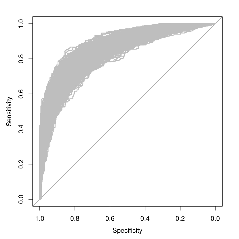
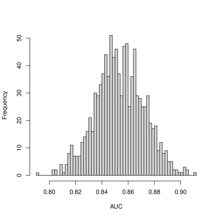
Figure 1: ROC curves (left plot) for the classification of main-shocks using the main-shock probabilities $\omega_{i}$ derived from the RETAS declustering algorithm applied to the simulated earthquake catalogs for the case where $\kappa=0.5$ and $\beta=2$. Histogram (right plot) of the AUC values for the ROC curves in the left plot.

Classification of an earthquake as either a main-shock or an aftershock is a binary classification problem, and therefore, the receiver operating characteristic (ROC) curve can be used to compare the estimated main-shock probabilities $\omega_{i}$ with the true main-shock labels. For each of the three situations described above, we calculate the ROC curves for all 1000 simulated catalogs and seven parameter specifications, and only show those for the RETAS model with $\kappa=0.5$ and $\beta=2$ in Figure 1 (left panel) using the declustering algorithm with the smoothed probabilities. The areas under the ROC curves (AUC) were calculated as well. The right panel of Figure 1 presents a histogram of the AUC values, which shows the consistently high AUC values and therefore the good performance of the declustering algorithm for main or aftershock classification.

The declustering algorithm provides accurate identification of main-shocks (hence also aftershocks) since consistently high AUC values are observed for the range of parameterizations

Table 4: Summary statistics for the AUC values for 1000 simulated earthquake catalogs with shape parameter $\kappa$ in the set $\left\{0.2,0.3,0.5,1,2,3,5\right\}$. The RETAS declustering algorithm was used to estimate the main-shock probabilities $\omega_{i}$ for the RETAS and then the ETAS declustering algorithm was used for both the RETAS and ETAS models.

		Min	1st Qu.	Median	Mean	3rd. Qu	Max.
$\kappa=0.2$	RETAS	0.8111	0.8742	0.8860	0.8848	0.8963	0.9263
	Filtered	0.7294	0.8004	0.8140	0.8137	0.8288	0.8783
	ETAS	0.5059	0.5814	0.6049	0.6067	0.6290	0.7306
$\kappa=0.3$	RETAS	0.8229	0.8623	0.8733	0.8727	0.8841	0.9137
	Filtered	0.7598	0.8258	0.8395	0.8385	0.8511	0.8952
	ETAS	0.6053	0.7392	0.7589	0.7571	0.7767	0.8366
$\kappa=0.5$	RETAS	0.7904	0.8413	0.8527	0.8536	0.8660	0.9108
	Filtered	0.7864	0.8309	0.8428	0.8430	0.8555	0.9058
	ETAS	0.7576	0.8110	0.8240	0.8239	0.8372	0.8828
$\kappa=1$	RETAS	0.7922	0.8531	0.8657	0.8647	0.8766	0.9151
	Filtered	0.7915	0.8532	0.8659	0.8649	0.8767	0.9153
	ETAS	0.7903	0.8537	0.8662	0.8652	0.8771	0.9156
$\kappa=2$	RETAS	0.8370	0.8859	0.8956	0.8951	0.9052	0.9476
	Filtered	0.8295	0.8788	0.8885	0.8883	0.8984	0.9457
	ETAS	0.8213	0.8722	0.8829	0.8826	0.8936	0.9416
$\kappa=3$	RETAS	0.8666	0.9046	0.9141	0.9138	0.9236	0.9483
	Filtered	0.8523	0.8911	0.9015	0.9009	0.9116	0.9432
	ETAS	0.8370	0.8786	0.8891	0.8889	0.8998	0.9362
$\kappa=5$	RETAS	0.8809	0.9258	0.9339	0.9334	0.9419	0.9677
	Filtered	0.8616	0.9026	0.9128	0.9117	0.9213	0.9523
	ETAS	0.8402	0.8828	0.8935	0.8927	0.9028	0.9354

as presented in Table 4. For comparison, we also present the results of the declustering algorithm based on the ETAS model. When $\kappa$ departs from one, the RETAS model consistently performs better at identifying main-shocks and has a more pronounced improvement when $\kappa$ departs further from one. For instance, when $\kappa=0.2$, the mean AUC for the RETAS model is $0.88$ while for the ETAS model it was significantly smaller at only $0.61$. When $\kappa=1$ the two models perform similarly as one would expect since the two models are very similar in this case (and would be identical if we imposed the restriction that $\hat{\kappa}=1$). The table also contains the results if the ETAS declustering algorithm discussed in Section 3.2 was applied for RETAS model declustering. The filtered probabilities have consistently poorer performance than the declustering algorithm based on the smoothed probabilities except when $\kappa=1$. However, the table suggest that selecting the correct model is more important than the declustering method used.

We also need to assess whether the declustering algorithm can recover the complete branching structure that includes the parent for each aftershock. For this purpose, we compare the main and aftershock probabilities derived from the declustering algorithm to the true simulated branching structure consisting of main-shock and parent labels. The most probable label classification for each earthquake $i=2,\dotsc,n$ based

Table 5: Summary statistics for the proportion of the entire branching structure inferred correctly (based on the most probable classification) for 1000 simulated earthquake catalogs with shape parameter $\kappa$ in the set $\left\{0.2,0.3,0.5,1,2,3,5\right\}$. The RETAS declustering algorithm was used to estimate the main-shock and parent probabilities $\left\{\omega_{i},\pi_{i,j},j=1,\dotsc,i-1\right\}$ for the RETAS and then the ETAS declustering algorithm was used for both the RETAS and ETAS models.

		Min.	1st Qu.	Median	Mean	3rd Qu.	Max.
$\kappa=0.2$	RETAS	0.5793	0.6320	0.6491	0.6494	0.6653	0.7408
	Filtered	0.5356	0.6031	0.6213	0.6215	0.6385	0.7242
	ETAS	0.4097	0.4654	0.4812	0.4827	0.5000	0.5787
$\kappa=0.3$	RETAS	0.6139	0.6612	0.6786	0.6785	0.6948	0.7566
	Filtered	0.5955	0.6485	0.6653	0.6656	0.6816	0.7500
	ETAS	0.4887	0.5782	0.5970	0.5972	0.6153	0.6901
$\kappa=0.5$	RETAS	0.5960	0.6694	0.6864	0.6870	0.7036	0.7833
	Filtered	0.5900	0.6661	0.6831	0.6839	0.6999	0.7757
	ETAS	0.5820	0.6515	0.6692	0.6692	0.6864	0.7573
$\kappa=1$	RETAS	0.6252	0.6936	0.7123	0.7111	0.7273	0.8018
	Filtered	0.6269	0.6938	0.7119	0.7111	0.7273	0.7995
	ETAS	0.6269	0.6946	0.7121	0.7115	0.7275	0.7995
$\kappa=2$	RETAS	0.6551	0.7137	0.7322	0.7317	0.7490	0.8124
	Filtered	0.6475	0.7124	0.7303	0.7298	0.7471	0.8101
	ETAS	0.6460	0.7066	0.7238	0.7238	0.7407	0.7963
$\kappa=3$	RETAS	0.6719	0.7260	0.7443	0.7442	0.7614	0.8434
	Filtered	0.6744	0.7241	0.7402	0.7404	0.7569	0.8434
	ETAS	0.6609	0.7132	0.7305	0.7298	0.7459	0.8361
$\kappa=5$	RETAS	0.6797	0.7381	0.7544	0.7547	0.7709	0.8390
	Filtered	0.6705	0.7284	0.7453	0.7456	0.7621	0.8277
	ETAS	0.6606	0.7142	0.7305	0.7304	0.7460	0.8186

on $\max\left\{\omega_{i},\pi_{ij},j=1,\dotsc,i-1\right\}$ is computed and compared with the true label from the simulations. Table 5 presents the proportion of the branching structure correctly inferred where a match is defined as the most probable index coinciding with the true parent or main-shock label. The RETAS delcustering algorithm based on the smooth probabilities correctly infers the majority of the branching structure with a mean proportion around $0.70$ for all parameter specifications under consideration. In some cases, the declustering algorithm can infer as much as $84\%$ of the branching structure correctly. By comparing with the ETAS model, it always has a superior performance and the largest improvement is seen when $\kappa$ is smallest ($\kappa=0.2$) in which there is a significant reduction of $0.17$ in the mean correct proportion inferred. Similar to Table 4, the filtered declustering algorithm has worse performance for all parameter specifications (when $\kappa$ departs from one) but its performance is still consistently better than the ETAS model results again suggesting that getting the model correct is more important.

5 Application to a New Zealand earthquake catalog

This section investigates a New Zealand (NZ) earthquake catalog from 1-Jan-1980 to 29-Feb-2020. The catalog was obtained from the GeoNet Quake Search Database and reports the hypocentral coordinates (longitude, latitude and time) and magnitude for 1173 earthquakes with threshold magnitude $m_{0}=5$. The coordinates $164^{\circ}-182^{\circ}$ E and $48^{\circ}-35^{\circ}$ S define the rectangular region $\mathcal{S}$, which was previously studied in Harte, (2013, 2014) and Stindl and Chen, (2021). The region covers all of New Zealand and hence different tectonic environments exists within the catalog.

Figure 2 displays the epicentral locations (left plot) and longitude-time occurrences (right plot) of earthquakes in the NZ catalog where the relative size of the magnitude is represented by the size of the circle. The figure shows strong evidence of heavy temporal and spatial clustering of the earthquakes. Seismic activity typically occurs where the Pacific Plate is subducting the Australian Plate in both the North Island and in the northern part of the South Island, the Australian Plate is subducting the Pacific Plate in the southwest of the South Island and the Alpine Fault which is located in the central part of the South Island (Harte,, 2013). The seismic activity is greatest closest to the tectonic boundaries and diminishes as one moves from the boundary to the west and east into the Tasman Sea and Pacific Ocean, respectively.

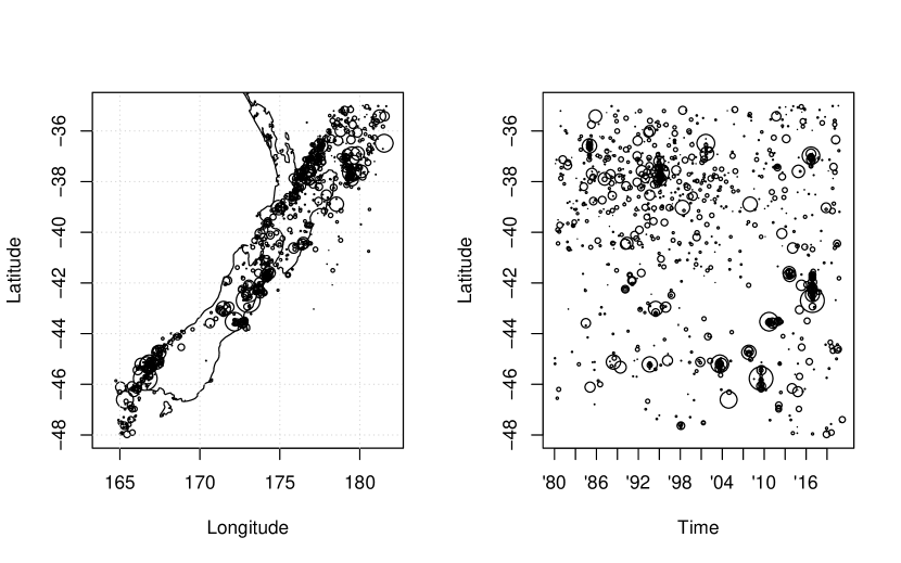
Figure 2: Epicentral locations (left plot) and latitude-time (right plot) plots for the NZ catalog where the relative size of the magnitude is indicated by the size of the circle.

The specific form of the RETAS model for this catalog is the same as described in Section 2. The semi-parametric iterative estimation algorithm is used to estimate the spatial intensity function $\nu(x,y)$ and the model parameters $\theta=(\kappa,\beta,p,c,\sigma_{1}^{2},\sigma_{2}^{2},A,\alpha)$, with the default smoothing parameter matrix multiplied by the factors $\zeta\in\left\{0.1,0.25,0.5,1,2,3,4\right\}$. The spatial intensity function is initialized using a 2d-KDE with equal weights assigned to all earthquakes in the catalog. The optimization routine to obtain the RETAS model parameters was initialized by fitting telescopically simpler models nested in the RETAS model. The parameter estimates, standard errors, productivity (Prod.), percentage of expected main-shocks (Pct), log-likelihood $\ell(\hat{\theta})$, effective number of parameters DoF for $\nu(x,y)$ and the AICc are provided in Table 6 for each adjustment factor. The magnitude density term in the likelihood function is separable, and its value is $-1410.97$ with $\hat{\gamma}=0.336$ and is the same in all cases and is not included in the tables calculation of $\ell(\hat{\theta})$.

Table 6: Estimation results for the semi-parametric estimation procedure with six different amounts of smoothing by multiplying the default smoothing matrix $h$ by factors of $\zeta$ in the set $\left\{0.1,25,0.5,1,2,3,4\right\}$ for the NZ catalog.

$\zeta$	$\kappa$	$\beta$	$p$	$c$	$\sigma_{1}^{2}$	$\sigma_{2}^{2}$	$A$	$\alpha$	Prod.	Pct	$\ell(\hat{\theta})$	DoF	AICc
0.1	0.853	25.61	1.165	0.00601	0.0168	0.00898	0.213	1.538	0.442	58.63	-4943.33	362.62	10845.20
	(0.0426)	(1.693)	(0.0219)	(0.00135)	(0.00165)	(0.00102)	(0.0196)	(0.0780)
0.25	0.850	26.50	1.136	0.00508	0.0170	0.00900	0.242	1.498	0.488	56.84	-5095.81	214.36	10721.73
	(0.0446)	(1.908)	(0.0191)	(0.000993)	(0.00168)	(0.00105)	(0.0294)	(0.0773)
0.5	0.848	27.25	1.115	0.00450	0.0172	0.00911	0.264	1.506	0.534	55.41	-5192.18	132.87	10709.65
	(0.0446)	(1.908)	(0.0191)	(0.000993)	(0.00168)	(0.00105)	(0.0294)	(0.0773)
1	0.844	28.26	1.091	0.00383	0.0174	0.009216	0.308	1.488	0.616	53.66	-5274.37	79.44	10745.47
	(0.0458)	(2.054)	(0.0186)	(0.000833)	(0.00170)	(0.00107)	(0.0432)	(0.0772)
2	0.839	29.58	1.0688	0.00328	0.0174	0.009315	0.384	1.443	0.738	51.63	-5346.27	45.65	10812.23
	(0.0473)	(2.251)	(0.0173)	(0.000678)	(0.00172)	(0.00108)	(0.0700)	(0.0783)
3	0.836	30.63	1.055	0.0030	0.0175	0.0094	0.461	1.411	0.877	50.00	-5386.93	32.42	10863.96
	(0.0486)	(2.409)	(0.0158)	(0.000587)	(0.00172)	(0.00110)	(0.100)	(0.0788)
4	0.831	31.70	1.043	0.00273	0.0177	0.00958	0.563	1.417	1.075	48.62	-5416.68	25.44	10907.63
	(0.0495)	(2.563)	(0.0147)	(0.000498)	(0.00173)	(0.00112)	(0.156)	(0.0775)

Table 6 exhibits similar patterns in parameter estimates to those observed in the simulation experiments as the amount of smoothing varies. The inference on the catalog changes substantially as $\zeta$ vaies. For example, the expected number of directly induced aftershocks, aka the productivity measure (Prod. in Table 6), $\mathbb{E}\big{[}Ae^{\alpha(m_{i}-m_{0})}\big{]}=A\gamma/(\gamma-\alpha)$ changes from the subcritical value of $0.442$ when $\zeta=0.1$ to the supercritical $1.075$ when $\zeta=4$. Moreover, the percentage of main-shocks (Pct in Table 6) also changed considerably from 58.63% when $\zeta=0.1$ to 48.62% when $\zeta=4$. The minimal AICc value is achieved when $\zeta=0.5$. We also investigated more extreme amounts of smoothing in both directions, and found that the AICc continues to increase. Therefore, we choose $\zeta=0.5$ as the optimal amount of smoothing and proceed with the analysis accordingly. The corresponding smoothing matrix $h=\bigl{(}\begin{smallmatrix}0.176&0.135\\ 0.135&0.118\end{smallmatrix}\bigr{)}$ is more or less in line with the amount of smoothing used in the work of Harte, (2013) selected by more ad hoc means.

The estimate of the main-shock spatial intensity function $\hat{\nu}(x,y)$ is presented in Figure 3. The majority of seismic background activity is occurring along the fault lines that go through NZ. There are two distinct seismically active regions that have significantly high incidence rate of main-shocks. Since we are dealing with a large space-time window, the earthquake process will generally be more heterogeneous than smaller space-time windows. Therefore, the rather flexible estimate for the spatial intensity function is necessary to capture the finer features of the fault lines.

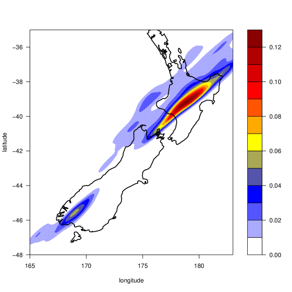
Figure 3: Estimate of the spatial intensity function $\hat{\nu}(x,y)$ from the final iteration of the semi-parametric estimation procedure with optimal amount of smoothing $\zeta=0.5$ using a weighted 2d-KDE for the NZ catalog.

The estimated model parameters and standard error estimates (in brackets) are as follows: $\hat{\kappa}=0.848\,\,(0.0446)$, $\hat{\beta}=27.24\,\,(1.908)$, $\hat{p}=1.115\,\,(0.0191)$, $\hat{c}=0.00450\,\,(0.000993)$, $\hat{\sigma}_{1}^{2}=0.0172\,\,(0.00168)$, $\hat{\sigma}_{2}^{2}=0.00911\,\,(0.00105)$, $\hat{A}=0.264\,\,(0.0294)$ and $\hat{\alpha}=1.506\,\,(0.0773)$. The estimates for the renewal main-shock arrival process $\hat{\kappa}$ and $\hat{\beta}$ implies a mean waiting time of 23.11 days (SE: 1.023) between main-shocks with a standard deviation of 25.09 days (SE: 1.291). The shape parameter $\kappa$ has a 95% confidence interval $(0.761,0.936)$ indicating it deviates significantly from unity which further suggests that the classical ETAS may not be sufficient to model the heavy temporal clustering of main-shocks. The estimates $\hat{A}$ and $\hat{\alpha}$ imply that the expected number of aftershocks induced by a size 5, 5.5, 6, 6.5 and 7 magnitude earthquake are 0.26, 0.56, 1.19, 2.52 and 5.35 earthquakes respectively with a productivity of 0.534.

Useful inferences can be drawn about the earthquake catalog based on the declustered main and aftershock probabilities. Since most of main-shock probabilities are close to either zero or one as seen in Figure 4, we can be reasonably confident in their main-shock classification. For instance, employing a threshold probability of $0.5$, there are $684$ $(58.31\%)$ earthquakes in the catalog that would be classified as a main-shock, or if we employ the most-probable classification (as we did in the numerical experiments) then there are $703$ $(59.93\%)$ main-shocks. In the work of Harte, (2013) main-shocks represented approximately $35\%$ of the catalog which is significantly lower than predicted by the RETAS model. One possible reason for this major disparity is that Harte, only examines shallow earthquakes (less than 40km deep) while our work deals with large magnitude earthquakes.

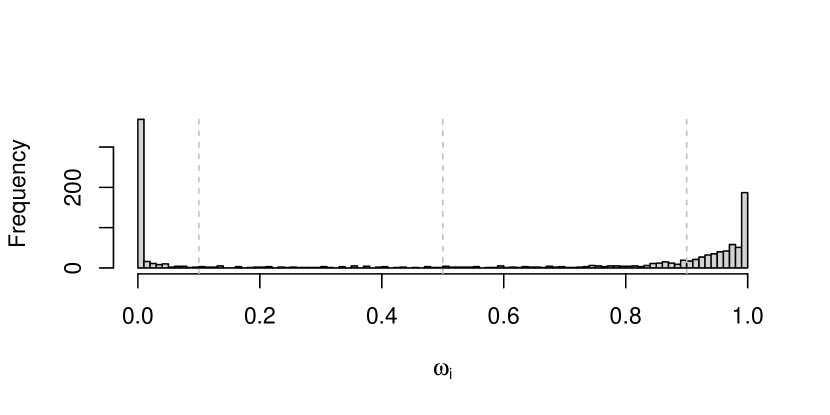
Figure 4: Frequency histogram of the main-shock probabilities $\omega_{i}$ implied by the RETAS model for the NZ catalog with the amount of smoothing $\zeta=0.5$.

The multi-generational structure implied by the fitted RETAS model is shown in Figure 5. From the $703$ main-shocks (using the most-probable classification), there were $73$ of these main-shocks which induced a first generation aftershock with a total of $180$ aftershocks among them. There was one main-shock which induced $25$ generation one aftershocks of its own, and we discuss this earthquake cluster next, as it is the most destructive earthquakes in the catalog. There were $46$ generation one aftershocks that induced a second generation, and 26 of these generated a third generation aftershock. There are several large clusters with many generations of aftershocks in the catalog. The largest cluster in the catalog begun on February 5th, 1995 at 22:51:02.31. It was located on the north-east region of New-Zealand ($171.49^{\circ}$ N and $37.65^{\circ}$ S, lower right plot in Figure 6) with a magnitude of 7.15 (being the fourth largest magnitude earthquake in the catalog). The declustering algorithm implies that this earthquake induced 25 aftershocks directly from it. There are a total of sixteen generations of aftershock that have resulted from this devastating earthquake. The size of the cluster (including the main-shock) is $84$ earthquakes with the second generation having $14$ earthquakes and the sixth generation having $7$ earthquakes.

The second largest cluster with $53$ aftershocks over $21$ generations (cf. upper right plot in Figure 6) originated on December 18th, 1984 at 11:16:58.12 at 177.57 ${}^{\circ}E$ and 36.63 ${}^{\circ}S$ with a main-shock magnitude of 5.24. Most aftershocks in this sequence only had one, two or three directly induced aftershocks, except for the earthquake that occurred two days later on December 30th, 1984 at 21:36:54 at 177.55 ${}^{\circ}E$ and 36.59 ${}^{\circ}S$ with magnitude $6.70$, which was a $13$-th generation of aftershock in the cluster, and induced directly $11$ aftershocks of its own. The third largest cluster had ten generations with a cluster size of $52$ and occurred in North Canterbury on November 13th, 2016 (see purple cluster in Figure 6).

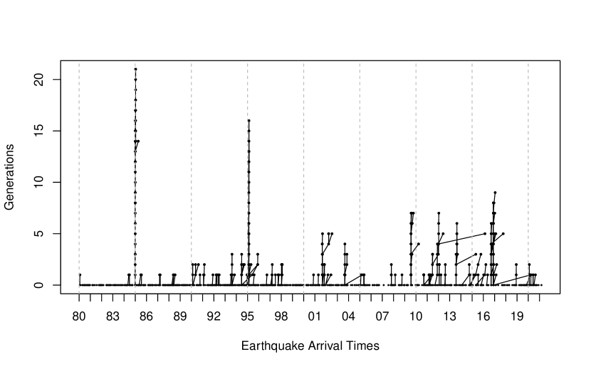
Figure 5: Multi-generation branching structure implied by the RETAS model for the NZ catalog with optimal amount of smoothing $\zeta=0.5$.

The largest magnitude earthquake occurred on November 13th, 2010 at 11:02:56 at $173.02^{\circ}$ N and $42.69^{\circ}$ S with a magnitude of $7.82$ (dark-blue cluster). It had five generations of aftershock with 15 aftershocks. The main-shock induced directly ten aftershocks on its own. The second largest magnitude at $7.80$ has seven generations of aftershock with a total cluster size of 40 (cyan cluster). In contrast, the third largest magnitude at $7.20$ only had one generation of aftershock with thirteen aftershocks (brown cluster).

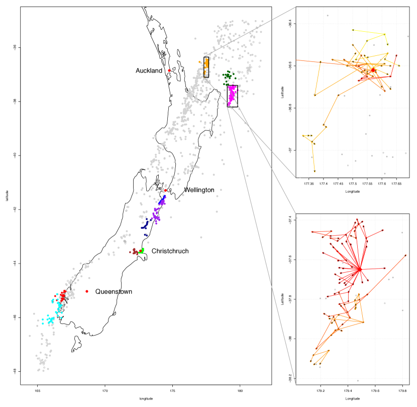
Figure 6: Left plot contains main-shock (solid circles) and aftershocks (open circles) based on fitted RETAS model. Several large clusters are represented by different colours on the plot. The two figures on the right are two large multi-generational aftershock sequences, in which the darker (lighter) shade arrows represent earlier (later) generation of aftershock.

Figure 6 shows several clusters that have been identified by the RETAS model with different colours representing the different clusters. The solid circles indicate main-shocks while the open circles indicate aftershocks. Some of the large clusters includes; Bay of Plenty in 1984-1985 (orange), East Cape in February 1995 (magenta), the Fiordland earthquake in August 2003 (red), Dusky Sound in July 2009 (cyan), Darfield in September 2010 known as the 2010 Canterbury earthquake (brown), Christchurch in February 2011 (green), Cook Strait in February 2011 which includes the 2013 Seddon earthquake (blue), NE of east Cape in September 2016 called the Te Araroa earthquake (dark-green), and two clusters in North Canterbury in November 2011 in which one contains the 2016 Kaikoura earthquake (dark-blue) and a second cluster (purple).

Appendix A Derivation of smoothed most recent main-shock probabilities $q_{ij}$

For compactness of notation, in the following, we define $z_{i}:=(t_{i},x_{i},y_{i},m_{i})$ as the time, coordinates and magnitude of the $i$th earthquake. The backward recursion smooths the filtered probabilities $p_{ij}=P(I(t_{i})=j|\mathcal{H}_{t_{i}-})$ calculated during likelihood evaluation based on weights derived from the conditional density $p(z_{i:n},t_{n+1}>T|\mathcal{H}_{t_{i}-},I(t_{i})=j)$ which follows from Bayes’ theorem

$$q_{ij} =\frac{p(z_{i:n},t_{n+1}>T\mid z_{1:i-1},I(t_{i})=j)}{\sum_{k=1}^{i-1}p\left(z_{i:n},t_{n+1}>T\mid z_{1:i-1},I(t_{i})=k\right)\,p_{ik}}\,p_{ij},$$ (22)

but its evaluation is not directly possible. For the purpose of evaluating (22), we denote $f_{ij}$ as the joint density of $z_{i:n}$ and $t_{n+1}>T$ conditional on $z_{1:i-1}$ and $I(t_{i})=j$, that is, $f_{ij}=p(z_{i:n},t_{n+1}>T|z_{1:i-1},I(t_{i})=j)$. Then there exists a relationship between the values $f_{ij}$ and $f_{i+1,j}$ by again applying Bayes’ theorem

$$f_{ij} =p(z_{i}|z_{1:i-1},I(t_{i})=j)\,p(z_{i+1:n},t_{n+1}>T\mid z_{1:i},I(t_{i})=j)$$

$$=\psi_{ij}\,\sum_{k=1}^{i}p(z_{i+1:n},t_{n+1}>T\mid z_{1:i},I(t_{i})=j,I(t_{i+1})=k)\,\mathbb{P}\left(I(t_{i+1})=k\mid z_{1:i},I(t_{i})=j\right)$$

where

$$\psi_{ij}=p(z_{i}\mid z_{1:i-1},I(t_{i})=j)=(\mu(t_{i}-t_{j})\nu(x_{i},y_{i})+\phi(t_{i}))e^{-\int_{t_{i-1}}^{t_{i}}\mu(s)\mathrm{d}s-\{\Phi(t_{i})-\Phi(t_{i-1})\}},$$

is the conditional density of $z_{i}$ conditioned on $z_{1:i-1}$ and $I(t_{i})=j$.

However, since the condition contains both $I(t_{i})=j$ and $I(t_{i+1})=k$, the only terms that contributes to the summation are when $k\in\left\{i,j\right\}$. Furthermore, since the main-shock renewal time at $t_{i+1}$ is included in the condition, the additional information $I(t_{i})=j$ in the condition is irrelevant as only the most recent renewal time provides information about the future evolution of the process conditional on the history. Therefore, calculation of $f_{ij}$ reduces to the following

$$f_{ij} =\psi_{ij}\,\sum_{k\in\left\{i,j\right\}}p(z_{i+1:n},t_{n+1}>T\mid z_{1:i},I(t_{i+1})=k)\,\mathbb{P}\left(I(t_{i+1})=k\mid z_{1:i},I(t_{i})=j\right)$$

$$=\psi_{ij}\,\sum_{k\in\left\{i,j\right\}}f_{i+1,k}\,\mathbb{P}\left(I(t_{i+1})=k\mid z_{1:i},I(t_{i})=j\right),$$ (23)

which depends on $f_{i+1,j}$. Since the most recent main-shock indicator function $I(t_{i+1})$ has two possible values $I(t_{i})$ or $i$ which depends on $B_{i}=0$ (main-shock) or $B_{i}=j$, $j<i$ (aftershock), $f_{ij}$ simplifies to the following

$$f_{ij} =\psi_{ij}\bigg{[}f_{i+1,j}\,\mathbb{P}\left(I(t_{i+1})=j\mid z_{1:i},I(t_{i})=j\right)+f_{i+1,i}\,\mathbb{P}\left(I(t_{i+1})=i\mid z_{1:i},I(t_{i})=j\right)\bigg{]}$$

$$=\psi_{ij}\bigg{[}f_{i+1,j}\,\mathbb{P}\left(B_{i}\neq 0\mid z_{1:i},I(t_{i})=j\right)+f_{i+1,i}\,\mathbb{P}\left(B_{i}=0\mid z_{1:i},I(t_{i})=j\right)\bigg{]}$$

$$=\psi_{ij}\bigg{[}f_{i+1,j}\,\frac{\phi(t_{i},x_{i},y_{i},m_{i})}{\mu(t_{i}-t_{j})\nu(x_{i},y_{i})+\phi(t_{i},x_{i},y_{i},m_{i})}+f_{i+1,i}\,\frac{\mu(t_{i}-t_{j})\nu(x_{i},y_{i})}{\mu(t_{i}-t_{j})\nu(x_{i},y_{i})+\phi(t_{i},x_{i},y_{i},m_{i})}\bigg{]}$$

$$=e^{-\int_{t_{i-1}}^{t_{i}}\mu(s-t_{j})\mathrm{d}s-(\Phi(t_{i})-\Phi(t_{i-1}))}\bigg{[}f_{i+1,j}\,\phi(t_{i},x_{i},y_{i},m_{i})+f_{i+1,i}\,\mu(t_{i}-t_{j})\nu(x_{i},y_{i})\bigg{]},$$ (24)

which depends on future values of $f_{i+1,j}$ and a backward recursion exists with starting condition

$$f_{n+1,j}=P(t_{n+1}>T|z_{1:n},t_{n+1}>T,I(t_{n+1})=j)=e^{-\int_{t_{n}}^{T}\mu(s-t_{j})\mathrm{d}s-\{\Phi(T)-\Phi(t_{n})\}}$$

for $j=1,\dotsc,n$. Hence, the smoothed most recent main-shock probabilities are given by

$$q_{ij}=\frac{f_{ij}}{\sum_{k=1}^{i-1}f_{ik}p_{ik}}\,p_{ij},$$ (25)

for $i=n,\dotsc,2$ and $j=1,\dotsc,i-1.$

Appendix B Derivation of smoothed branching structure probabilities $\omega_{i}$ and $\pi_{ij}$

First, by applying Bayes’ theorem, the smoothed main-shock probabilities $\omega_{ij}$ are given by

$$\omega_{ij} =\mathbb{P}(B_{i}=0,I(t_{i})=j|z_{1:n},t_{n+1}>T)$$

$$=\mathbb{P}\left(B_{i}=0|z_{1:n},t_{n+1}>T,I(t_{i})=j\right)\,\mathbb{P}\left(I(t_{i})=j|z_{1:n},z_{n+1}>T\right)$$

$$=\frac{p(z_{i+1:n},t_{n+1}>T|z_{1:i},B_{i}=0,I(t_{i})=j)\,\mathbb{P}\left(M_{i}=0|z_{1:i},I(t_{i})=j\right)}{p(z_{i+1:n},t_{n+1}>T|z_{1:i},I(t_{i})=j)}\,q_{ij}$$

$$=\frac{p(z_{i+1:n},t_{n+1}>T|z_{1:i},I(t_{i+1})=i)\,\mathbb{P}\left(B_{i}=0|z_{1:i},I(t_{i})=j\right)}{p(z_{i+1:n},t_{n+1}>T|z_{1:i},I(t_{i})=j)}\,q_{ij}.$$ (26)

Then applying a similar simplification to that used in (24) and the definition of $f_{ij}$ the following holds

$$\omega_{ij}=\frac{f_{i+1,i}\,\mu(t_{i}-t_{j})\nu(x_{i},y_{i})}{f_{i+1,j}\,\phi(t_{i},x_{i},y_{i},m_{i})+f_{i+1,i}\,\mu(t_{i}-t_{j})\nu(x_{i},y_{i})}\,q_{ij},$$ (27)

for which the smoothed main-shock probability is obtained by summing over all possible indices

$$\omega_{i}=\sum_{j=1}^{i-1}\omega_{ij}.$$ (28)

Calculation of the smoothed aftershock probabilities $\pi_{ij}$ are calculated by again applying Bayes’ theorem and take the form

$$\pi_{ij} =\mathbb{P}\left(B_{i}=j|z_{1:n},t_{n+1}>T\right)$$

$$=\sum_{k=1}^{i-1}\mathbb{P}\left(B_{i}=j|z_{1:n},t_{n+1}>T,I(t_{i})=k\right)\,q_{ik}$$

$$=\sum_{k=1}^{i-1}\frac{p(z_{i+1:n},t_{n+1}>T|z_{1:i},I(t_{i})=k,B_{i}=j)\,\mathbb{P}\left(B_{i}=j|z_{1:i},I(t_{i})=k\right)}{p(z_{i+1:n},t_{n+1}>T\mid z_{1:i},I(t_{i})=k)}\,q_{ik}$$

The denominator in the above expression has already been calculated in (A) and implies the following expression to calculate $\pi_{ij}$

$$\pi_{ij} =\sum_{k=1}^{i-1}\frac{p(z_{i+1:n},t_{n+1}>T\mid z_{1:i},I(t_{i+1})=k)\,\frac{k(m_{i})g(t_{i}-t_{j})f(x_{i}-x_{j},y_{i}-y_{j})}{\mu(t_{i}-t_{k})\nu(x_{i},y_{i})+\phi(t_{i},x_{i},y_{i},m_{i})}}{f_{i+1,k}\,\frac{\phi(t_{i},x_{i},y_{i},m_{i})}{\mu(t_{i}-t_{k})\nu(x_{i},y_{i})+\phi(t_{i},x_{i},y_{i},m_{i})}+f_{i+1,i}\,\frac{\mu(t_{i}-t_{k})\nu(x_{i},y_{i})}{\mu(t_{i}-t_{k})\nu(x_{i},y_{i})+\phi(t_{i},x_{i},y_{i},m_{i})}}\,q_{ik}$$

$$=\sum_{k=1}^{i-1}\frac{f_{i+1,k}\,k(m_{i})g(t_{i}-t_{j})f(x_{i}-x_{j},y_{i}-y_{j})}{f_{i+1,k}\,\phi(t_{i},x_{i},y_{i},m_{i})+f_{i+1,i}\,\mu(t_{i}-t_{k})\nu(x_{i},y_{i})}\,q_{ik}.$$ (29)

References

- Akaike, (1971) Akaike, H. (1971). Autoregressive model fitting for control. Annals of the Institute of Statistical Mathematics, 23(1):163–180.
- Burnham and Anderson, (2002) Burnham, K. P. and Anderson, D. R. (2002). A practical information-theoretic approach. Model selection and multimodel inference, 2:70–71.
- Chen and Stindl, (2018) Chen, F. and Stindl, T. (2018). Direct likelihood evaluation for the renewal Hawkes process. Journal of Computational and Graphical Statistics, 27(1):119–131.
- Cheng et al., (2018) Cheng, Y., Dundar, M., and Mohler, G. (2018). A coupled ETAS-I2GMM point process with applications to seismic fault detection. The Annals of Applied Statistics, 12(3):1853 – 1870.
- Clark and Dixon, (2018) Clark, N. J. and Dixon, P. M. (2018). Modeling and estimation for self-exciting spatio-temporal models of terrorist activity. Ann. Appl. Stat., 12(1):633–653.
- Console et al., (2003) Console, R., Murru, M., and Lombardi, A. M. (2003). Refining earthquake clustering models. Journal of Geophysical Research: Solid Earth, 108(B10).
- (7) Fox, E. W., Schoenberg, F. P., and Gordon, J. S. (2016a). Spatially inhomogeneous background rate estimators and uncertainty quantification for nonparametric Hawkes point process models of earthquake occurrences. The Annals of Applied Statistics, 10(3):1725 – 1756.
- (8) Fox, E. W., Short, M. B., Schoenberg, F. P., Coronges, K. D., and Bertozzi, A. L. (2016b). Modeling e-mail networks and inferring leadership using self-exciting point processes. Journal of the American Statistical Association, 111(514):564–584.
- Guo et al., (2015) Guo, Y., Zhuang, J., and Zhou, S. (2015). An improved space-time etas model for inverting the rupture geometry from seismicity triggering. Journal of Geophysical Research: Solid Earth, 120(5):3309–3323.
- Gutenberg and Richter, (1944) Gutenberg, B. and Richter, C. F. (1944). Frequency of earthquakes in California. Bulletin of the Seismological Society of America, 34(4):185–188.
- Harte, (2013) Harte, D. S. (2013). Bias in fitting the etas model: a case study based on New Zealand seismicity. Geophysical Journal International, 192(1):390–412.
- Harte, (2014) Harte, D. S. (2014). An etas model with varying productivity rates. Geophysical Journal International, 198(1):270–284.
- Hurvich and Tsai, (1989) Hurvich, C. M. and Tsai, C.-L. (1989). Regression and time series model selection in small samples. Biometrika, 76(2):297–307.
- McCloud and Parmeter, (2020) McCloud, N. and Parmeter, C. F. (2020). Determining the number of effective parameters in kernel density estimation. Computational Statistics & Data Analysis, 143:106843.
- Meyer et al., (2012) Meyer, S., Elias, J., and Höhle, M. (2012). A space—time conditional intensity model for invasive meningococcal disease occurrence. Biometrics, 68(2):607–616.
- Mohler, (2014) Mohler, G. (2014). Marked point process hotspot maps for homicide and gun crime prediction in chicago. International Journal of Forecasting, 30(3):491 – 497.
- Mohler et al., (2011) Mohler, G. O., Short, M. B., Brantingham, P. J., Schoenberg, F. P., and Tita, G. E. (2011). Self-exciting point process modeling of crime. Journal of the American Statistical Association, 106(493):100–108.
- Musmeci and Vere-Jones, (1992) Musmeci, F. and Vere-Jones, D. (1992). A space-time clustering model for historical earthquakes. Annals of the Institute of Statistical Mathematics, 44(1):1–11.
- Ogata, (1988) Ogata, Y. (1988). Statistical models for earthquake occurrences and residual analysis for point processes. Journal of the American Statistical Association, 83(401):9–27.
- Ogata, (1998) Ogata, Y. (1998). Space-time point-process models for earthquake occurrences. Annals of the Institute of Statistical Mathematics, 50(2):379–402.
- Ogata, (2011) Ogata, Y. (2011). Significant improvements of the space-time etas model for forecasting of accurate baseline seismicity. Earth, Planets and Space, 63(3):6.
- Omori, (1894) Omori, F. (1894). On the aftershocks of earthquakes. Jounal of the College of Science, Imperial University of Tokyo, 7:111–120.
- Peng et al., (2005) Peng, R. D., Schoenberg, F. P., and Woods, J. A. (2005). A space–time conditional intensity model for evaluating a wildfire hazard index. Journal of the American Statistical Association, 100(469):26–35.
- Reid, (1910) Reid, H. F. (1910). The california earthquake of April 18, 1906. Volume II. The Mechanics of the Earthquake. Washington DC: Carnegie Institution of Washington, Publication No. 87.
- Schoenberg et al., (2019) Schoenberg, F. P., Hoffmann, M., and Harrigan, R. J. (2019). A recursive point process model for infectious diseases. Annals of the Institute of Statistical Mathematics, 71(5):1271–1287.
- Stindl and Chen, (2021) Stindl, T. and Chen, F. (2021). Spatiotemporal etas model with a renewal main-shock arrival process. arXiv preprint arXiv:2112.07861.
- Utsu, (1961) Utsu, T. (1961). A statistical study on the occurrence of aftershocks. Geophysical magazine, 30:521–605.
- Wand and Jones, (1994) Wand, M. P. and Jones, M. C. (1994). Multivariate plug-in bandwidth selection. Computational Statistics, 9(2):97–116.
- Wheatley et al., (2016) Wheatley, S., Filimonov, V., and Sornette, D. (2016). The Hawkes process with renewal immigration its estimation with an EM algorithm. Computational Statistics Data Analysis, 94:120 – 135.
- Zhuang and Mateu, (2019) Zhuang, J. and Mateu, J. (2019). A semiparametric spatiotemporal hawkes-type point process model with periodic background for crime data. Journal of the Royal Statistical Society: Series A (Statistics in Society), 182(3):919–942.
- Zhuang et al., (2002) Zhuang, J., Ogata, Y., and Vere-Jones, D. (2002). Stochastic declustering of space-time earthquake occurrences. Journal of the American Statistical Association, 97(458):369–380.
- Zipkin et al., (2016) Zipkin, J. R., Schoenberg, F. P., Coronges, K., and Bertozzi, A. L. (2016). Point-process models of social network interactions: Parameter estimation and missing data recovery. European Journal of Applied Mathematics, 27(3):502–529.