Aesthetic Attribute Assessment of Images Numerically on Mixed Multi-attribute Datasets

Abstract.

With the continuous development of social software and multimedia technology, images have become a kind of important carrier for spreading information and socializing. How to evaluate an image comprehensively has become the focus of recent researches. The traditional image aesthetic assessment methods often adopt single numerical overall assessment scores, which has certain subjectivity and can no longer meet the higher aesthetic requirements. In this paper, we construct an new image attribute dataset called aesthetic mixed dataset with attributes(AMD-A) and design external attribute features for fusion. Besides, we propose a efficient method for image aesthetic attribute assessment on mixed multi-attribute dataset and construct a multitasking network architecture by using the EfficientNet-B0 as the backbone network. Our model can achieve aesthetic classification, overall scoring and attribute scoring. In each sub-network, we improve the feature extraction through ECA channel attention module. As for the final overall scoring, we adopt the idea of the teacher-student network and use the classification sub-network to guide the aesthetic overall fine-grain regression. Experimental results, using the MindSpore, show that our proposed method can effectively improve the performance of the aesthetic overall and attribute assessment.

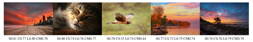
Figure 1. The examples for image aesthetic attribute assessment, S represents the overall score, C represents the color score, L represents the light score, and CM represents the composition score

1. Introduction

The visual aesthetic quality of the image measures the visual attraction of the images for humans. Since visual aesthetics is a subjective attribute (Kairanbay et al., 2019), it always depends on personal emotions and preferences. This makes image aesthetic quality assessment a subjective task and evaluated only by experts. If there is a large number of image samples, the efficiency of artificial aesthetic quality assessment will be quite low. However, people tend to agree that some images do indeed more attractive than others in daily life, which creates a computational aesthetics (Datta et al., 2006). Computational aesthetics lets the computer mimic the process of human aesthetic assessment and compute the methods to predict the aesthetic quality of the images automatically.

The focus of computational aesthetics is to predict people’s emotional responses to visual stimuli through computational technology, study the internal mechanism of human perception and explore the mystery of artificial aesthetic intelligence. Computational visual aesthetics (Brachmann and Redies, 2017) is the computational processing of human visual information. Image aesthetic assessment is the most popular research direction in the field of computational visual aesthetics, and it is also the first step in studying computational visual aesthetics. Image aesthetic assessment is to simulate human perception and cognition by the computers, which can provide the quantitative assessment of aesthetic quality. Image aesthetic attributes assessment mainly focuses on the quantitative assessment formed by aesthetic attributes such as composition, color and light in the photographic images.

There are two main parts for the image aesthetics quality assessment: the feature extraction part and the assessment part. In the feature extraction, Yan et al. (Ke et al., 2006) proposed the 7-dimensional aesthetic features based on photography knowledge and high-level semantics. The features include simplicity, spatial edges distribution, color distribution, hue count, blur, contrast and brightness. With the development of deep learning, researchers introduce deep convolutional neural networks in the task of image aesthetics assessment. Due to the ability of learning features automatically, people can extract aesthetic features from images by the deep convolutional neural networks without a lot of aesthetic knowledge and professionally photography experiences. However, there are deficiencies in general aesthetic benchmark datasets. For example, in AADB (Kong et al., 2016a), each image is only marked by a small number of annotation. So the data labels is kind of subjective. It is difficult to extract the aesthetic attribute features and limits the extraction ability of features for the model. At the same time, the multidimensional attribute assessment will lead to a sharp increase in the number of network parameters, which is not conducive to the actual development and application.

To solve these problems, we propose a efficient method for image aesthetic attribute assessment based on the mixed multi-attribute dataset. Our work includes the following three contributions:

1. We screen and construct the aesthetic mixed dataset with attributes(AMD-A), which has more image aesthetic attribute annotations compared with the traditional aesthetic attribute datasets.

2. We propose an aesthetic multitasking network architecture based on EfficientNet-B0 and ECA channel attention modules to simplify the model parameters and realize the aesthetic classification, overall scoring and attribute scoring.

3. We design several kinds of external attribute features and use feature fusion to imporve the performance of the image aesthetic attribute assessment. Besides, inspired by teacher-student network, we propose the soft loss to imporve the performance of the image aesthetic overall assessment.

2. Related work

2.1. Image aesthetic assessment

Image aesthetic assessment is usually regarded as a classification or score regression task. For the classification task, images can generally be divided into high-quality images and low-quality images (Sperry et al., 1969). For the regression task, images can be evaluated according to aesthetic overall scores. However, the overall scores can not accurately measure the results of aesthetic assessment, which largely ignores the diversity, subjectivity, and personality in the human aesthetic consensus. An image also contains many aesthetic attributes such as light and shadow, color, composition, blur, movement, and interest. So the related work has focused on the multidimensional aesthetic attribute assessment.

In the early stage, the handcraft designing features was the main way to extract features from images (Tong et al., 2004; Luo and Tang, 2008; Nishiyama et al., 2011; Marchesotti et al., 2011a). Datta et al. (Datta et al., 2006) used bottom-level features (color, texture, shape, image size, etc.) and high-level features (depth of field, rule of thirds, regional contrast) as the image aesthetic features. Marchesotti (Marchesotti et al., 2011b) and others directly used SIFT (BOV or FisherVector) and local color descriptors to classify aesthetic images.

Today, deep learning has been widely used in different walks of life, such as IoV (Wang et al., 2022a), IoT (Wang et al., 2022b) and edge intelligence (Zhang et al., 2020). With the development of deep learning, the researchers introduce deep convolutional neural networks into the image aesthetic assessment. Due to the powerful learning capabilities in deep convolutional neural networks, people can automatically extract aesthetic features without substantial theoretical knowledge and photographic experience. In recent years, deep convolutional neural networks have shown good performance in the overall regression and classification tasks of image aesthetics, and a series of excellent models (Ma et al., 2017; Kao et al., 2015; Deng et al., 2018; She et al., 2021; Zhou et al., 2022b; Xu et al., 2022; Zhen et al., 2022) have emerged. At the same time, in the field of image aesthetic attribute assessment, there are image aesthetic attribute scoring methods based on hierarchical multitasking networks (Jin et al., 2018) and incremental learning multitasking networks (Jin et al., 2019) by using image composition, light and color, exposure depth of field and other attributes. However, due to the limitation of data quantity and the categories of aesthetic attributes, the above attribute assessment method don’t have high accuracy. With the increasing of attribute categories, the network models become extremely complex, which is not conducive to expansion and practical application.

2.2. Aesthetic attribute datasets

The emergence of large-scale aesthetic datasets provides a rich source of samples for aesthetic assessment model training. Murray et al. (Murray et al., 2012) constructed an aesthetic visual analysis dataset(AVA), containing 255,530 images from the www.dpchallenge.com. AVA is the benchmark dataset for the current image aesthetic quality assessment task. Each image includes a numerical aesthetic overall regression label, 66 semantic labels, and 14 style labels. Building on this dataset, Kang et al. (Kang et al., 2020) proposed the explainable visual aesthetics dataset(EVA), which contains 4070 images. Each image has 30 annotation scores at least and mainly includes an overall score and 4 different aesthetic attribute scores. Compared with AVA, EVA adopts a more rigorous annotation collection method and overcomes the noisy labels due to the misunderstanding bias of the annotators, which facilitates the research on aesthetic understanding.

Kong et al. (Kong et al., 2016a) designed the aesthetics and attributes database(AADB). The dataset contains 9958 images from professional photographers and ordinary photographers, each image has an overall score and eleven aesthetic attributes scores. Chang et al. (Chang et al., 2017) first proposed the annotation information for aesthetic language assessment, and designed the photo critique captioning dataset(PCCD), which contains 4235 valid images from the foreign photography website Gurushots.com. Except for the overall score, each image has language comments and scores on the composition perspective, color illumination, image theme, depth of field, focus, and camera use. Fang et al. (Fang et al., 2020) conducted the first systematic study on the smartphone image aesthetic quality assessment and constructed smartphone photography attribute and quality dataset(SPAQ). The dataset consists of 11125 images taken by 66 smartphones, and each image including an overall label, an image attribute label and a scene category label.

2.3. Feature fusion

Feature fusion is a common way to improve the model performance. In the field of aesthetic assessment, the low-level features obtained by deep neural networks have high resolution and contain more aesthetic low-level information, such as color, texture and structure. But after fewer convolutional layers, low-level features contain lower high-level semantics and are easy to cause noise interference (Zhou et al., 2022a; Zhou et al., 2019). High-level features tend to have stronger semantic information, but they have very low feature resolution and poor perception of details. In the aesthetic field, local aesthetic attributes based on low-level information are as important as global aesthetic features based on high-level information. Especially in the regression task of aesthetic attributes. The output results of deep convolutional networks are often in the last layer of the network, which leads to the inability to effectively extract the corresponding attribute features in the assessment of aesthetic attributes.

In related work, the researchers improve the performance of detecting and dividing objects by integrating the network layer features at different locations of the neural network. We classified feature fusion and predicted output as early and late fusion. The idea of early fusion strategy is to integrate the high-level and low-leve features, and then conduct model training and prediction on the fusion features. Such methods usually use concatting and adding operations to fuse the features. Related research work such as Inside-Outside Net (Bell et al., 2016) and HyperNet (Kong et al., 2016b). The idea of the late fusion strategy is to output the prediction results of different network layers and then to fuse all the detection results. Related research work such as Feature Pyramid Network (Lin et al., 2017), Single Shot MultiBox Detector (Liu et al., 2016), and Densenet (Huang et al., 2017). This paper mainly adopts the early fusion strategy to integrate different high-level features of the sub-networks and external attribute features to improve the supervised assessment performance of image aesthetic attributes.

3. Aesthetic mixed dataset with attributes(AMD-A)

In order to construct a dataset with a reasonable distribution both in image aesthetics quality assessment and image aesthetic attributes assessment, we rebuild a dataset named Aesthetic mixed dataset with attributes(AMD-A) cincluding 16924 images. According to different tasks, AMD-A is divided into two sets. One set(11166 images) is applied to aesthetic overall score regression, another set(16924 images) is applied to aesthetic attribute score classification and regression.

As for the attribute regression, we collect images from EVA (Kang et al., 2020), AADB (Kong et al., 2016a), PCCD (Chang et al., 2017), PADB, and HADB. PADB and HADB are self-built datasets. Each image has three attribute labels and one overall label for assessment. The three attributes include light, color and composition. To increase the training samples of the aesthetic regression, we collected 5758 images with only overall scores from other datasets. There are from DPCallenge.com, SCUI-FBP5500 (Liang et al., 2018), Photo.net and SPAQ (Fang et al., 2020). Data labels are continuous and each one has a score range of 0-1. The distribution of different labels are as Fig.2.

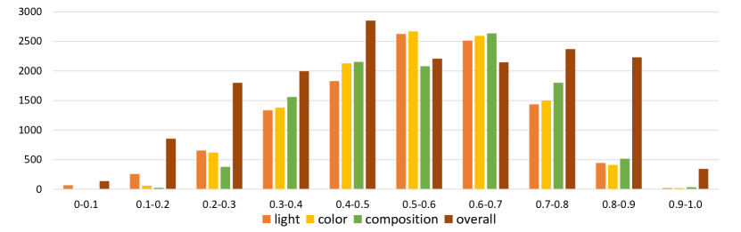
Figure 2. The distribution of light, color, composition and overall labels in AMD-A

We calculated the means and the standard deviations of the labels in Table 1. The results show that the 4 different categories of labels have the similar data distributions.

Table 1. Means and standard deviations for light, color, composition and overall labels

	light	color	composition	overall
Mean	0.5324	0.5472	0.5420	0.5398
Standard deviation	0.1522	0.1319	0.1388	0.2116

4. Network architecture

We build a multitasking network architecture including the backbone network and five sub-networks. The basic network architecture is shown in Fig.3.

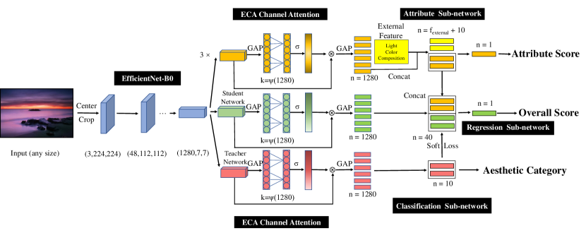
Figure 3. The architecture of the network

We use EfficientNet-B0 as the backbone network (Tan and Le, 2019). EfficientNet has an efficient feature extraction ability and can achieve more accurate aesthetic regression with a small number of parameters. The size of the parameter model for EffiecinetNet-B0 is only 20M, which is smaller than many existing model parameter model. So it is an ideal pre-trained parameter model in development and application scenarios. We use the blue part for the backbone network in the fig.3.

Between the backbone network and the sub-networks, there are ECA channel attention modules. In ECA, GAP is the global average pooling, $\sigma$ is the sigmoid function, $\psi(C)$ is the function of parameter k, and each layer will be activated by the relu function. We will introduce it in Section 4.1.

The five sub-networks are one classification sub-network, three attribute sub-networks and one regression sub-network consisting of fully connected layers. We use the red part for the classification sub-network, the khaki part for the attribute sub-networks and the green part for the regression sub-network. The attribute sub-networks in the figure have the similar structure, so we omitted additional attribute sub-networks and displayed only one attribute sub-network. The yellow part is for the external attribute features(4 light features, 7 color features, and 10 composition features).

From the architecture of the network, we can see two different kinds of feature fusions. One for external features and 10 attribute features in the attribute regression tasks, and another one for 10 regression features and 30 attribute features in the regression task. The training details will be explained in Section 4.2.

4.1. ECA channel attention

From the network structure in Fig.3, each ECA channel attention module is added between the backbone network and each sub-network. Recently, there are a lot of researches improving channel and spatial attention to make progresses in the performance. The ECA channel attention can improve the ability of extracting features. It mainly improves from the SENet (Qilong Wang and Hu., 2020) module. ECA channel attention proposes a local cross-channel interaction strategy without the dimension reduction and implement a method of adaptively selecting the size of the one-dimensional convolution kernel. So we use it to improve the performance of the image aesthetic attribute and overall assessment. To the best of our knowledge, it is also the first time to use the ECA channel attention in the task of aesthetics attribute assessment.

Instead of reducing global average pooling layers at the channel level, ECA channel attention captures local cross-channel interaction information by considering each channel and its k neighbors. This can be effectively achieved efficiently by a fast one-dimensional convolution. k indicates how many neighbors near the channel participate in the attention prediction of this channel. To avoid artificially raising k by cross-validation, (Qilong Wang and Hu., 2020) proposes a way to determine k automatically. The size of the convolutional kernel k is proportional to the channel dimension as follows:

(1) $$k=\psi(C)\ =\left|\frac{\log_{2}(C)}{\gamma}+\frac{b}{\gamma}\right|_{\mathrm{odd}}$$

${|t|}_{odd}$ means the nearest odd number of t, the value of $\gamma$ is 2, the value of b is 1. We can get k = 7 if C = 1280.

4.2. Multitasking network

We use EfficientNet-B0 as the backbone network and design the classification sub-network for the classification task. Between these two networks, we use the ECA channel attention module to improve the capability of the aesthetic feature extraction. The classification task divides aesthetic images into ten categories based on the level of aesthetic scores, which is a coarse-grained aesthetic regression. During training, we relaxed the parameters of the backbone network and the classification sub-network, obtained the high-level aesthetic features of 1280×7×7 through the EfficientNet-B0, and made the feature reweighted through the ECA channel attention module. After that, we used the global average pooling layer to transform the high-level features into 1280 features, then reduced the features to 10 through one full connection layer and the activation function. Each feature of the output is the probability of each aesthetic category.

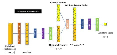
Figure 4. Attribute feature fusion

After completing the classification task, we trained the three sub-networks in the order of light, color and composition. The training labels are the attribute labels of each image. The structure of attribute sub-networks are similar to the classification sub-networks. We reduced 1280 features to 10 features by one fully connected layer and the activation function. These 10 features are the attribute features of the image. As shown in Fig.4, we spliced different external features onto attribute features and regress the features to an attribute score using one fully connected layer and the activation function. The design and calculation of the external features will be mentioned in Section 5.

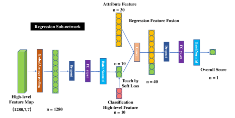
Figure 5. Overall feature fusion

(2) $$Loss=MSELoss+\lambda\texttimes SoftLoss$$

As shown in Fig.5, we also reduced 1280 features to 10 features in the regression sub-network. Then, we combined these 10 features with 3×10 attribute features in the penultimate layer of the attribute sub-network to obtain an aesthetic overall score through one fully connected layer and the activation function. Inspired by the idea of teacher-student networks (Hinton et al., 2015), we used 10 features from the output of the classification sub-network to guide the 10 features of the regression sub-network. We calculate the relative entropy between the two feature sequences and define it as the soft loss. The regression sub-network is gradient-adjusted by the mse loss of the aesthetic score regression and a weighted soft loss. We set the weight of the soft loss as 0.1, which we will prove in Section 6.

5. Attribute Features Fusion

Before training the three attribute regression sub-networks, we will design and calculate the external attribute features of the input images. The external attribute features includes light features, color features and composition features. We will store the external attribute features in the data labels. The design details are presented in this section.

5.1. Light features

Referring to the value and lightness information (Datta et al., 2006), we extract the light features as mean of value(f1), standard deviation of value(f2), mean of lightness(f3) and standard deviation of lightness(f4).

The light features was mainly obtained by calculating the mean and standard deviation of the L and V channels. Both the value and lightness range is 0-255. We use x to represent the pixels in the images. The calculation formulas of average brightness (f1), standard deviation of brightness (f2), average lightness (f3) and standard deviation of lightness (f4) are as follows:

(3) $$f_{1}=\frac{1}{|I|}{\mathrm{\sum}_{x\in{I}}L(x)}$$

(4) $$f_{2}=std(L(x))$$

(5) $$f_{3}=\frac{1}{|I|}{\mathrm{\sum}_{x\in{I}}V(x)}$$

(6) $$f_{4}=std(V(x))$$

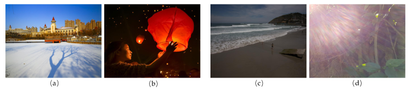
Figure 6. Samples with different light effects

Table 2. Light feature values for samples

Light feature	6(a)	6(b)	6(c)	6(d)
Mean of value (f1)	148.253016	34.985529	72.411960	139.248896
Standard deviation of value (f2)	52.104682	40.385166	29.037064	39.939841
Mean of lightness (f3)	183.823056	148.253016	79.659121	151.227269
Standard deviation of lightness (f4)	50.643524	78.682690	28.775265	43.909947

Fig.6 shows four sample images of different light effects, where Fig.6(a) and Fig.6(b) have better light effects, while Fig.6(c) and Fig.6(d) have poor light effect. Table 2 shows the light feature values corresponding to these four images. From the feature values in Table 2, we can see that the images with better light effect generally have higher means and standard deviations. While the image is too dark, the means and standard deviations are lower, and if the exposure is too excessive, the means will be higher and the standard deviations will be lower.

5.2. Color features

Referring to the color information (Azimi et al., 2012), we extract the color features as the weight of color channel (f1), the number of RGB dominant colors (f2), the degree of RGB dominant colors (f3), the number of HSV dominant colors (f4), the degree of HSV dominant colors (f5), the number of dominant hues (f6), the contrast ratio of dominant hues (f7).

By calculating the approximation degree of the RGB color channel, the images can be divided into colored three-channel images, approximate grayscale channel images and grayscale single-channel images. The weight of color channel f1 is calculated by converting the image into the RGB channels. If the values of the three channel are exactly the same, f1 = 0. If the three channels are not exactly consistent, we will calculate the average difference between the RGB channels at each pixel, while the average difference is less than 10, f1 = 0.5; otherwise, the images are considered as the colored three-channel images, and f1 = 1.

The dominant colors are mainly calculated by the color histogram in the RGB channel and the hue histogram in the HSV channel. As for RGB dominant colors, we quantize each RGB channel to 8 values, so that a 512-dimensional histogram h_RGB={h₀, h₁,…, h₅₁₁} can be created. h_i represents the number of pixels in the i-th histogram. c₁ is the threshold parameter of the color number in the formula and c₁ = 0.01, which means if the number of the color in RGB is more then 51, and we can consider it as the RGB dominant color. We define the number of RGB dominant colors (f2) as follows:

(7) $$f_{2}=\sum_{k=0}^{512}1\left(h_{k}\geq c_{1}\max_{i}h_{i}\right)$$

The degree of RGB dominant colors (f3) indicates that how the dominant color is occupied in the image colors. The formula is as follows:

(8) $$f_{3}=\frac{\max_{i}h_{i}}{|I|}$$

Similarly, replacing the RGB channel with the HSV channel, we can get the number of HSV dominant colors (f4) and the degree of HSV dominant colors (f5).

For f6 and f7, we eliminated pixels with saturation elimination values less than 0.2, in other words, we eliminated all light or dark pixels. We then calculate the hue histograms of the remaining pixels with 20 uniform intervals, each occupying 18° sectors of the hue ring. In the hue histogram H_hue = {h₀, h₁, …, h₁₉}, h_i represents the pixel histogram in the i-th interval. The formula for the number of dominant hues is as follows:

(9) $$f_{6}=\sum_{i=1}^{20}\mathbf{1}\left(\left|h_{i}\right|\geq c_{2}|I|\right)$$

Similarly, we set c₂ = 0.01. The contrast ratio of dominant hues (f7) indicates the maximum contrast between the two principal hues in the image, the formula is as follows:

(10) $$f_{7}=\max_{i,j}\left\|\left|h_{i}\right|-\left|h_{j}\right|\right\|$$

Fig.7 shows four sample images of different color effects, where Fig.7(a) and Fig.7(b) have better color effects, while Fig.7(c) and Fig.7(d) have poor color effect. Table 3 shows the color feature values corresponding to these four images. From the feature values in Table 3, we can see that the images with better color effect generally have more RGB and HSV dominant colors. Besides, the degree and the contrast ratio is higher. So we can find that the images have the better color effects when they have richer colors.

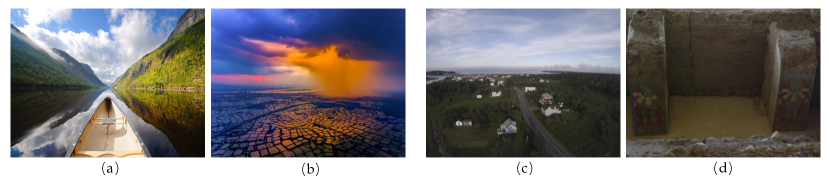
Figure 7. Color feature values for samples

Table 3. Calculation results of Color feature sample

Color feature	7(a)	7(b)	7(c)	7(d)
Weight of color channel f1	1.0	1.0	1.0	1.0
Number of RGB dominant colors f2	102	100	19	14
Degree of RGB dominant colors f3	0.087823	0.075602	0.253429	0.228055
Number of HSV dominant colors f4	220	171	49	39
Degree of HSV dominant colors f5	0.040854	0.052193	0.160361	0.197352
Number of dominant hues f6	8	10	5	4
Contrast ratio of dominant hues f7	162	162	18	18

5.3. Composition Features

We extract the composition features as golden section (f1), center (f2), slant (f3), the triangle (f4), guideline (f5), rule of thirds (f6), symmetry (f7), diagonal (f8), frame (f9) and circle (f10).

For the composition features f1 and f2, we first obtain the salient area of the images through salient detection (Liu et al., 2020), and then calculate the distance d from the golden section and central points of the image according to the central position of the pixel coordinates in the significance area. After that, we divide the distance d by the oblique length of the image to indicate the proximity to the composition. To numerically represent the positive correlation of the compositional feature values, we subtract this value by 1 and represent it as f1 and f2. The formula of the features is as follows:

(11) $$f_{1,2}=1-\frac{d}{\sqrt{w^{2}+h^{2}}}$$

We obtain the composition feature line of the images by the model in (Han et al., 2020) and calculate f3-f6. Firstly, we determine the composition feature lines according to the rule of thirds line, symmetrical line, diagonal line and slash line. Then, we respectively calculate the distances between the two endpoints of each composition feature line and the two endpoints of the composition feature line, divide them by the long side of the image and average them. Finally, we subtract this value with 1 to represent the compositional feature calculated values.To better distinguish the accuracy of the values, we set a threshold as 0.3, above which yields a positive value, or 0 otherwise. The calculation formula for f3-f6 is as follows:

(12) $$f_{3-6}=1-\frac{d_{1}+d_{2}}{2\max(w,h)}$$

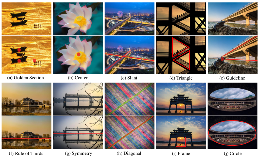
Figure 8. Samples with diffenrent composition effects

Table 4. Composition feature values for samples

Composition feature	11(a)	11(b)	11(c)	11(d)	11(e)	11(f)	11(g)	11(h)	11(i)	11(j)
Golden Section f1	0.67	0	0	0	0	0	0	0	0	0
Center f2	0	0.85	0	0	0	0.66	0.76	0	0.69	0.70
Slant f3	0	0	0.48	0	0.41	0	0	0.71	0	0
Triangle f4	0	0	0	0.44	0	0	0	0	0	0
Guildline f5	0	0	0	0	0.71	0	0	0	0	0
Rule of Thirds f6	0	0	0	0	0.48	0.84	0	0	0	0
Symmetry f7	0	0	0	0	0	0	1	0	0	0
Diagonal f8	0	0	0	0	0	0	0	1	0	0
Frame f9	0	0	0	0	0	0	0	0	1	0
Circle f10	0	0	0	0	0	0	0	0	0	1

We obtained features f7-f9 by calculating whether the intersection positions of the main composition lines are within the range of the images. If there is an intersection of the composition feature line on the image, we will calculate the horizontal angle of the composition feature line. If more than a pair of horizontal angles are complementary, and the distances between the intersections of the composition feature lines are within 0.05max(w, h), f7 = 1. If the sum of any three composition feature lines and the horizontal surface is 360° and its intersection are within the image, we will consider it as the triangle composition, f8 = 1. If two composition feature lines are approximately parallel in the horizontal or vertical direction, and another composition feature line is almost vertical to them at the same time, then we will consider it as the frame composition, f9 = 1. If we detect the image by the hough circle and get the radius of the circle is longer than 0.1min (w, h), we will consider it as the circle composition, f10 = 1. Otherwise all the above features f7-f10 are 0.

Fig.8 shows ten sample images of different composition effects. Table 4 shows the composition feature values corresponding to these ten images. From the feature values in Table 4, we can see that the images with one or more than one composition features have better composition effects.

5.4. Feature fusion

The network structure in Fig.3 shows that the yellow part is the external attribute feature f_external(4 for light features, 7 for color features or 10 for composition features). We concat these features with the aesthetic high-level features extracted from the backbone network by the method mentioned in Section 4.2. The experiment results in Section 6 verify the method of the feature fusion.

6. Experiment

6.1. Training details

We set the classification batch size to be 32, the regression batch size to be 64 and the learning rate to be 0.0001. We use Adam as the optimizer; betas are set as (0.98, 0.999); weight decay is set as 0.0001. If the accuracy rate of classification is not improved in two consecutive rounds, or the regression loss is not decreased in two consecutive rounds, the learning rate will multiply by 0.5. Our running environment is in MindSpore (MindSpore, 2022) 1.6.0 and Nvidia TITAN XPs. We divide the dataset into three sets; the ratio of training set and validation set and testing set is 8:1:1.

6.2. Analysis of results

This paper uses several indicators to measure training results:

MSE mean square error represents the estimating errors of the difference between the predicted results and the true values; the formula is:

(13) $$MSE=\frac{1}{N}\sum_{i}{(r_{i}-\widehat{r_{i}})}^{2}$$

SROCC (Spearman rankorder correlation coefficient, Spearman rank correlation coefficient) represents the correlation between the predicted result and the true value and the formula is:

(14) $$SROCC=1-\frac{6\sum_{i}{(r_{i}-\widehat{r_{i}})}^{2}}{N^{3}-N}$$

The accuracy of the two-classification indicates whether the predicted score and the real score are consistent when the boundary is 5. The accuracy of two-classification indicates the most basic accuracy of classification; the formula is:

(15) $$ACCURACY=\frac{TP+TN}{P+N}$$

The positive and negative accuracy indicates whether the absolute value of the error is within 1 point between the predicted score and the real score. If the absolute value of the error is within 1 point, the result can be considered accurate. The formula is:

(16) $$ACCURACY_{\left|error\right|\leq 1}=\frac{N_{\left|error\right|\leq 1}}{N}$$

Table 5. Feature fussion experimental results

Methods	Attributes	MSE	SROCC	Acc	$Acc_{\left|error\right|\leq 1}$
	Color	0.008660	0.6863	76.17%	73.68%
Baseline (Mindspore)	Light	0.011266	0.6939	77.72%	68.29%
	Composition	0.009491	0.6915	77.41%	70.57%
Basebone +	Color	0.008307	0.7087	77.72%	73.69%
Feature fusion	Light	0.010675	0.7126	79.27%	69.53%
(Mindspore)	Composition	0.009285	0.7013	79.79%	73.47%

Table 6. Soft loss experimental results

Methods	Attributes	MSE	SROCC	Acc	$Acc_{\left|error\right|\leq 1}$
Baseline (Mindspore)	Score	0.012940	0.8424	85.78%	64.99%
Baseline + Soft loss (Mindspore)	Score	0.011315	0.8604	88.08%	68.72%

We use EfficientNet-B0 as the baseline and conducte several experiments as follows: for feature fusion, Table 5 showed that external light, color, and composition attribute features could return to a more accurate assessment after fusion. For overall score regression, we used the soft loss mentioned in Section 4.2, and Table 6 showed that the model with soft loss had better performances in all indicators.

Table 7. The comparison experiment for $\lambda$

$\lambda$	MSE	SROCC	Acc	$Acc_{\left|error\right|\leq 1}$
0	0.011408	0.8591	88.02%	68.31%
0.1	0.011315	0.8604	88.08%	68.72%
0.2	0.011318	0.8603	87.88%	68.44%
0.3	0.011402	0.8595	87.81%	68.58%
0.4	0.011437	0.8591	87.74%	68.45%

We did a comparison experiment in 40 epoches of training. Table 7 showes that the presence of $\lambda$ does improve the accuracy of the regression, when $\lambda$ = 0.1, so we set $\lambda$ to 0.1.

Besides, we selected some typical samples and used this method to score the images, including the overall aesthetic score and the scores of the three aesthetic attributes. Among them, S represents the overall score, C represents the color score, L represents the light score, and CM represents the composition score, as shown in Fig.9:

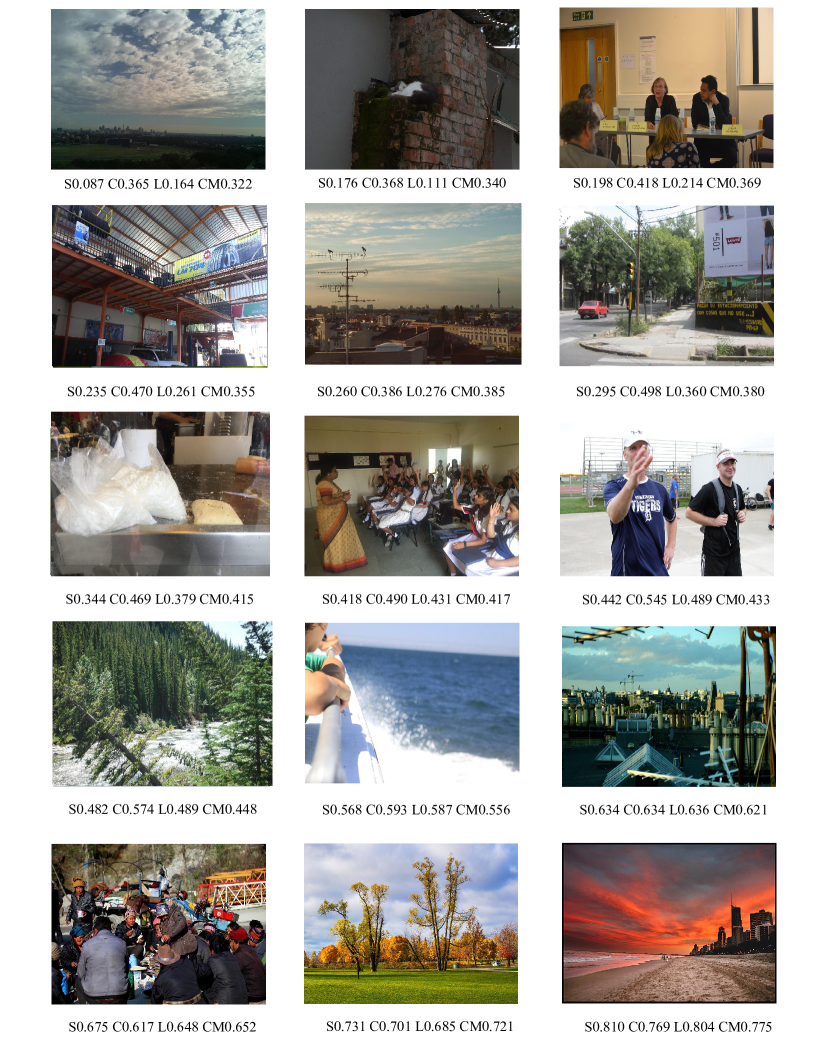
Figure 9. Test samples on the testing set with scores from low to high. S represents the overall score, C represents the color score, L represents the light score, and CM represents the composition score

7. Summarize

It is challenging to construct a new dataset in the image aesthetic quality assessment. Traditional datasets have the problem of few data and limited attribute labels. By mixing and filtering massive datasets and designing external attribute features, we get a new dataset called aesthetic mixed dataset with attributes(AMD-A) with a more reasonable distribution. Besides, we propose a model with multitasking network including one classification sub-network, three attribute sub-network and one regression sub-network. This is an innovative exploration of the training method for the numerical assessment of image aesthetics. Moreover, we design and use the external attribute feature fusion to improve the regressing of aesthetic attributes. According to the idea of the teacher-student network, we use the classification sub-network to guide the regression sub-network through high-level features by the soft loss. The experimental results proved that our model is more accurate than the traditional deep learning network regression model, and it improves the prediction of aesthetic attributes and overall scores.

References

- (1)
- Azimi et al. (2012) Javad Azimi, Ruofei Zhang, Yang Zhou, Vidhya Navalpakkam, Jianchang Mao, and Xiaoli Fern. 2012. The impact of visual appearance on user response in online display advertising. In proceedings of the 21st international conference on World Wide Web. 457–458.
- Bell et al. (2016) Sean Bell, C Lawrence Zitnick, Kavita Bala, and Ross Girshick. 2016. Inside-outside net: Detecting objects in context with skip pooling and recurrent neural networks. In Proceedings of the IEEE conference on computer vision and pattern recognition. 2874–2883.
- Brachmann and Redies (2017) Anselm Brachmann and Christoph Redies. 2017. Computational and experimental approaches to visual aesthetics. Frontiers in computational neuroscience 11 (2017), 102.
- Chang et al. (2017) Kuang-Yu Chang, Kung-Hung Lu, and Chu-Song Chen. 2017. Aesthetic critiques generation for photos. In Proceedings of the IEEE international conference on computer vision. 3514–3523.
- Datta et al. (2006) Ritendra Datta, Dhiraj Joshi, Jia Li, and James Z Wang. 2006. Studying aesthetics in photographic images using a computational approach. In European conference on computer vision. Springer, 288–301.
- Deng et al. (2018) Yubin Deng, Chen Change Loy, and Xiaoou Tang. 2018. Aesthetic-driven image enhancement by adversarial learning. In Proceedings of the 26th ACM international conference on Multimedia. 870–878.
- Fang et al. (2020) Yuming Fang, Hanwei Zhu, Yan Zeng, Kede Ma, and Zhou Wang. 2020. Perceptual quality assessment of smartphone photography. In Proceedings of the IEEE/CVF Conference on Computer Vision and Pattern Recognition. 3677–3686.
- Han et al. (2020) Qi Han, Kai Zhao, Jun Xu, and Ming-Ming Cheng. 2020. Deep Hough Transform for Semantic Line Detection. In European Conference on Computer Vision (ECCV). 249–265. https://doi.org/10.1007/978-3-030-58545-7_15
- Hinton et al. (2015) Geoffrey Hinton, Oriol Vinyals, Jeff Dean, et al. 2015. Distilling the knowledge in a neural network. arXiv preprint arXiv:1503.02531 2, 7 (2015).
- Huang et al. (2017) Gao Huang, Zhuang Liu, Laurens Van Der Maaten, and Kilian Q Weinberger. 2017. Densely connected convolutional networks. In Proceedings of the IEEE conference on computer vision and pattern recognition. 4700–4708.
- Jin et al. (2018) Xin Jin, Le Wu, Xinghui Zhou, Geng Zhao, Xiaokun Zhang, Xiaodong Li, and Shiming Ge. 2018. Predicting aesthetic radar map using a hierarchical multi-task network. In Chinese Conference on Pattern Recognition and Computer Vision (PRCV). Springer, 41–50.
- Jin et al. (2019) Xin Jin, Xinghui Zhou, Xiaodong Li, Xiaokun Zhang, Hongbo Sun, Xiqiao Li, and Ruijun Liu. 2019. Incremental Learning of Multi-Tasking Networks for Aesthetic Radar Map Prediction. IEEE Access 7 (2019), 183647–183655.
- Kairanbay et al. (2019) Magzhan Kairanbay, John See, and Lai-Kuan Wong. 2019. Beauty is in the eye of the beholder: Demographically oriented analysis of aesthetics in photographs. ACM Transactions on Multimedia Computing, Communications, and Applications (TOMM) 15, 2s (2019), 1–21.
- Kang et al. (2020) Chen Kang, Giuseppe Valenzise, and Frédéric Dufaux. 2020. EVA: An Explainable Visual Aesthetics Dataset. In Joint Workshop on Aesthetic and Technical Quality Assessment of Multimedia and Media Analytics for Societal Trends. 5–13.
- Kao et al. (2015) Yueying Kao, Chong Wang, and Kaiqi Huang. 2015. Visual aesthetic quality assessment with a regression model. In 2015 IEEE International Conference on Image Processing (ICIP). IEEE, 1583–1587.
- Ke et al. (2006) Yan Ke, Xiaoou Tang, and Feng Jing. 2006. The design of high-level features for photo quality assessment. In 2006 IEEE Computer Society Conference on Computer Vision and Pattern Recognition (CVPR’06), Vol. 1. IEEE, 419–426.
- Kong et al. (2016a) Shu Kong, Xiaohui Shen, Zhe Lin, Radomir Mech, and Charless Fowlkes. 2016a. Photo aesthetics ranking network with attributes and content adaptation. In European conference on computer vision. Springer, 662–679.
- Kong et al. (2016b) Tao Kong, Anbang Yao, Yurong Chen, and Fuchun Sun. 2016b. Hypernet: Towards accurate region proposal generation and joint object detection. In Proceedings of the IEEE conference on computer vision and pattern recognition. 845–853.
- Liang et al. (2018) Lingyu Liang, Luojun Lin, Lianwen Jin, Duorui Xie, and Mengru Li. 2018. SCUT-FBP5500: a diverse benchmark dataset for multi-paradigm facial beauty prediction. In 2018 24th International Conference on Pattern Recognition (ICPR). IEEE, 1598–1603.
- Lin et al. (2017) Tsung-Yi Lin, Piotr Dollár, Ross Girshick, Kaiming He, Bharath Hariharan, and Serge Belongie. 2017. Feature pyramid networks for object detection. In Proceedings of the IEEE conference on computer vision and pattern recognition. 2117–2125.
- Liu et al. (2020) Jiang-Jiang Liu, Qibin Hou, and Ming-Ming Cheng. 2020. Dynamic feature integration for simultaneous detection of salient object, edge, and skeleton. IEEE Transactions on Image Processing 29 (2020), 8652–8667.
- Liu et al. (2016) Wei Liu, Dragomir Anguelov, Dumitru Erhan, Christian Szegedy, Scott Reed, Cheng-Yang Fu, and Alexander C Berg. 2016. Ssd: Single shot multibox detector. In European conference on computer vision. Springer, 21–37.
- Luo and Tang (2008) Yiwen Luo and Xiaoou Tang. 2008. Photo and video quality evaluation: Focusing on the subject. In European conference on computer vision. Springer, 386–399.
- Ma et al. (2017) Shuang Ma, Jing Liu, and Chang Wen Chen. 2017. A-lamp: Adaptive layout-aware multi-patch deep convolutional neural network for photo aesthetic assessment. In Proceedings of the IEEE conference on computer vision and pattern recognition. 4535–4544.
- Marchesotti et al. (2011a) Luca Marchesotti, Florent Perronnin, Diane Larlus, and Gabriela Csurka. 2011a. Assessing the aesthetic quality of photographs using generic image descriptors. In 2011 international conference on computer vision. IEEE, 1784–1791.
- Marchesotti et al. (2011b) Luca Marchesotti, Florent Perronnin, Diane Larlus, and Gabriela Csurka. 2011b. Assessing the aesthetic quality of photographs using generic image descriptors. In 2011 international conference on computer vision. IEEE, 1784–1791.
- MindSpore (2022) MindSpore. 2022. https://www.mindspore.cn/.
- Murray et al. (2012) Naila Murray, Luca Marchesotti, and Florent Perronnin. 2012. AVA: A large-scale database for aesthetic visual analysis. In 2012 IEEE conference on computer vision and pattern recognition. IEEE, 2408–2415.
- Nishiyama et al. (2011) Masashi Nishiyama, Takahiro Okabe, Imari Sato, and Yoichi Sato. 2011. Aesthetic quality classification of photographs based on color harmony. In CVPR 2011. IEEE, 33–40.
- Qilong Wang and Hu. (2020) Pengfei Zhu Peihua Li Wangmeng Zuo Qilong Wang, Banggu Wu and Qinghua Hu. 2020. ECA-Net: Efficient Channel Attention for Deep Convolutional Neural Networks. (2020), 11531––11539.
- She et al. (2021) Dongyu She, Yu-Kun Lai, Gaoxiong Yi, and Kun Xu. 2021. Hierarchical layout-aware graph convolutional network for unified aesthetics assessment. In Proceedings of the IEEE/CVF Conference on Computer Vision and Pattern Recognition. 8475–8484.
- Sperry et al. (1969) R. W. Sperry, M. S. Gazzaniga, and J. E. Bogen. 1969. Interhemispheric relationships: the neocortical commissures; syndromes of hemisphere disconnection. Handbook of Clinical Neurology 4 (1969), 145–153.
- Tan and Le (2019) Mingxing Tan and Quoc Le. 2019. Efficientnet: Rethinking model scaling for convolutional neural networks. In International conference on machine learning. PMLR, 6105–6114.
- Tong et al. (2004) Hanghang Tong, Mingjing Li, Hong-Jiang Zhang, Jingrui He, and Changshui Zhang. 2004. Classification of digital photos taken by photographers or home users. In Pacific-Rim Conference on Multimedia. Springer, 198–205.
- Wang et al. (2022a) Ranran Wang, Yin Zhang, Giancarlo Fortino, Qingxu Guan, Jiangchuan Liu, and Jeungeun Song. 2022a. Software Escalation Prediction Based on Deep Learning in the Cognitive Internet of Vehicles. IEEE TRANSACTIONS ON INTELLIGENT TRANSPORTATION SYSTEMS (2022).
- Wang et al. (2022b) Ranran Wang, Yin Zhang, Limei Peng, Giancarlo Fortino, and Pin-Han Ho. 2022b. Time-varying-aware network traffic prediction via deep learning in IIoT. IEEE Transactions on Industrial Informatics (2022).
- Xu et al. (2022) Liming Xu, Xianhua Zeng, Weisheng Li, and Bochuan Zheng. 2022. MFGAN: Multi-modal Feature-fusion for CT Metal Artifact Reduction Using GANs. ACM Transactions on Multimedia Computing, Communications, and Applications (TOMM) (2022).
- Zhang et al. (2020) Yin Zhang, Yujie Li, Ranran Wang, Jianmin Lu, Xiao Ma, and Meikang Qiu. 2020. PSAC: Proactive sequence-aware content caching via deep learning at the network edge. IEEE Transactions on Network Science and Engineering 7, 4 (2020), 2145–2154.
- Zhen et al. (2022) Peining Zhen, Shuqi Wang, Suming Zhang, Xiaotao Yan, Wei Wang, Zhigang Ji, and Hai-Bao Chen. 2022. Towards Accurate Oriented Object Detection in Aerial Images with Adaptive Multi-level Feature Fusion. ACM Transactions on Multimedia Computing, Communications, and Applications (TOMM) (2022).
- Zhou et al. (2022a) Quan Zhou, Xiaofu Wu, Suofei Zhang, Bin Kang, Zongyuan Ge, and Longin Jan Latecki. 2022a. Contextual ensemble network for semantic segmentation. Pattern Recognition 122 (2022), 108290.
- Zhou et al. (2019) Quan Zhou, Wenbing Yang, Guangwei Gao, Weihua Ou, Huimin Lu, Jie Chen, and Longin Jan Latecki. 2019. Multi-scale deep context convolutional neural networks for semantic segmentation. World Wide Web 22, 2 (2019), 555–570.
- Zhou et al. (2022b) Wei Zhou, Zhiwu Xia, Peng Dou, Tao Su, and Haifeng Hu. 2022b. Double Attention based on Graph Attention Network for Image Multi-Label Classification. ACM Transactions on Multimedia Computing, Communications, and Applications (TOMM) (2022).