Preparations for Quantum Simulations of Quantum Chromodynamics in $1+1$ Dimensions: (I) Axial Gauge

Abstract

Tools necessary for quantum simulations of $1+1$ dimensional quantum chromodynamics are developed. When formulated in axial gauge and with two flavors of quarks, this system requires 12 qubits per spatial site with the gauge fields included via non-local interactions. Classical computations and D-Wave’s quantum annealer Advantage are used to determine the hadronic spectrum, enabling a decomposition of the masses and a study of quark entanglement. Color “edge” states confined within a screening length of the end of the lattice are found. IBM’s 7-qubit quantum computers, ibmq_jakarta and ibm_perth, are used to compute dynamics from the trivial vacuum in one-flavor QCD with one spatial site. More generally, the Hamiltonian and quantum circuits for time evolution of $1+1$ dimensional $SU(N_{c})$ gauge theory with $N_{f}$ flavors of quarks are developed, and the resource requirements for large-scale quantum simulations are estimated.

I Introduction

Simulations of the real-time dynamics of out-of-equilibrium, finite density quantum systems is a major goal of Standard Model (SM) [1, 2, 3, 4, 5, 6] physics research and is expected to be computed efficiently [7] with ideal quantum computers [8, 9, 10, 11, 12, 13, 14, 15, 16]. For recent reviews, see Refs. [17, 18, 19]. Developing such capabilities would enable precision predictions of particle production and fragmentation in beam-beam collisions at the LHC and RHIC, of the matter-antimatter asymmetry production in the early universe, and of the structure and dynamics of dense matter in supernova and the neutrino flavor dynamics therein. They would also play a role in better understanding protons and nuclei, particularly their entanglement structures and dynamics, and in exploring exotic strong-interaction phenomena such as color transparency. First steps are being taken toward simulating quantum field theories (QFTs) using currently available, NISQ-era (Noisy Intermediate Scale Quantum) quantum devices [20], by studying low-dimensional and truncated many-body systems (see for example, Refs. [21, 22, 23, 24, 25, 26, 27, 28, 29, 30, 31, 32, 33, 34, 35, 36, 37, 38, 39, 40, 41, 42, 43, 44, 45, 46, 47, 48, 49, 35, 50, 51, 52, 53, 54, 55, 56, 57, 58, 59, 60, 61, 62, 63, 64, 65, 66, 67, 68, 69, 70, 71, 72, 73, 74, 75, 76]). These studies are permitting first quantum resource estimates to be made for more realistic simulations.

There has already been a number of quantum simulations of latticized $1+1$D quantum electrodynamics (QED, the lattice Schwinger model), starting with the pioneering work of Martinez et al. [25]. The Schwinger model shares important features with quantum chromodynamics (QCD), such as charge screening, a non-zero fermion condensate, nontrivial topological charge sectors and a $\theta$-term. Quantum simulations of the Schwinger model have been performed using quantum computers [25, 77, 31, 78, 79, 66], and there is significant effort being made to extend this progress to higher dimensional QED [80, 81, 82, 83, 84, 85, 86, 87, 88, 89, 90, 23, 91, 28, 92, 93, 94, 60, 73]. These, of course, build upon far more extensive and detailed classical simulations of this model and analytic solutions of the continuum theory. There is also a rich portfolio of classical and analytic studies of $1+1$D $SU(N_{c})$ gauge theories [95, 96, 97, 98, 99], with some seminal papers preparing for quantum simulations [100, 101, 102, 103, 82, 104, 35, 50, 93], with the recent appearance of quantum simulations of a 1-flavor ($N_{f}=1$) $1+1$D $SU(2)$ lattice gauge theory [105]. An attribute that makes such calculations attractive for early quantum simulations is that the gauge field(s) are uniquely constrained by Gauss’s law at each lattice site. However, this is also a limitation for understanding higher dimensional theories where the gauge field is dynamical. After pioneering theoretical works developing the formalism and also end-to-end simulation protocols nearly a decade ago, it is only recently that first quantum simulations of the dynamics of a few plaquettes of gauge fields have been performed [35, 50, 105, 71].

Due to its essential features, quantum simulations of the Schwinger model provide benchmarks for QFTs and quantum devices for the foreseeable future. Moving toward simulations of QCD requires including non-Abelian local gauge symmetry and multiple flavors of dynamical quarks. Low-energy, static and near-static observables in the continuum theory in $1+1$D are well explored analytically and numerically, with remarkable results demonstrated, particularly in the ’t Hooft model of large-$N_{c}$ [106, 107] where the Bethe-Salpeter equation becomes exact. For a detailed discussion of $1+1$D $U(1)$ and $SU(N_{c})$ gauge theories, see Refs. [108, 109]. Extending such calculations to inelastic scattering to predict, for instance, exclusive processes in high-energy hadronic collisions is a decadal challenge.

In $3+1$D QCD, the last 50 years have seen remarkable progress in using classical high-performance computing to provide robust numerical results using lattice QCD, e.g., Refs. [110, 111], where the quark and gluon fields are discretized in spacetime. Lattice QCD is providing complementary and synergistic results to those obtained in experimental facilities, moving beyond what is possible with analytic techniques alone. However, the scope of classical computations, even with beyond-exascale computing platforms [112, 113, 110], is limited by the use of a less fundamental theory (classical) to simulate a more fundamental theory (quantum).

Building upon theoretical progress in identifying candidate theories for early exploration (e.g., Ref. [114]), quantum simulations of $1+1$D non-Abelian gauge theories including matter were recently performed [105] for a $N_{c}=2$ local gauge symmetry with one flavor of quark, $N_{f}=1$. The Jordan-Wigner (JW) mapping [115] was used to define the lattice theory, and Variational Quantum Eigensolver (VQE) [116] quantum circuits were developed and used on IBM’s quantum devices [117] to determine the vacuum energy, along with meson and baryon masses. Further, there have been previous quantum simulations of 1- and 2-plaquette systems in $N_{c}=2,3$ Yang-Mills lattice gauge theories [118, 119, 120, 57, 74] that did not include quarks. Simulations of such systems are developing rapidly [120, 71] due to algorithmic and hardware advances. In addition, distinct mappings of these theories are being pursued [121, 122, 123, 124, 125, 126, 127].

This work focuses on the quantum simulation of $1+1$D $SU(N_{c})$ lattice gauge theory for arbitrary $N_{c}$ and $N_{f}$. Calculations are primarily done in $A^{(a)}_{x}=0$ axial (Arnowitt-Fickler) gauge, which leads to non-local interactions in order to define the chromo-electric field contributions to the energy density via Gauss’s law. This is in contrast to Weyl gauge, $A_{t}^{(a)}=0$, where contributions remain local. The resource estimates for asymptotic quantum simulations of the Schwinger model in Weyl gauge have been recently performed [129], and also for Yang-Mills gauge theory based upon the Byrnes-Yamamoto mapping [130]. Here, the focus is on near-term, and hence non-asymptotic, quantum simulations to better assess the resource requirements for quantum simulations of non-Abelian gauge theories with multiple flavors of quarks. For concreteness, $N_{f}=2$ QCD is studied in detail, including the mass decomposition of the low-lying hadrons (the $\sigma$- and $\pi$-meson, the single baryon and the two-baryon bound state), color edge-states, entanglement structures within the hadrons and quantum circuits for time evolution. Further, results are presented for the quantum simulation of a $N_{f}=1$, single-site system, using IBM’s quantum computers [117]. Such quantum simulations will play a critical role in evolving the functionality, protocols and workflows to be used in $3+1$D simulations of QCD, including the preparation of scattering states, time evolution and subsequent particle detection. As a step in this direction, in a companion to the present paper, the results of this work have been applied to the quantum simulation of $\beta$-decay of a single baryon in $1+1$D QCD [131]. Motivated by the recent successes in co-designing efficient multi-qubit operations in trapped-ion systems [132, 133], additional multi-qubit or qudit operations are identified, specific to lattice gauge theories, that would benefit from being native operations on quantum devices.

II QCD with Three Colors and Two flavors in $1+1$D

In $3+1$D, the low-lying spectrum of $N_{f}=2$ QCD is remarkably rich. The lightest hadrons are the $\pi$s, which are identified as the pseudo-Goldstone bosons associated with the spontaneous breaking of the approximate global $SU(2)_{L}\otimes SU(2)_{R}$ chiral symmetry, which becomes exact in the chiral limit where the $\pi$s are massless. At slightly higher mass are the broad $I=0$ spinless resonance, $\sigma$, and the narrow $I=0$, $\omega$, and $I=1$, $\rho$, vector resonances as well as the multi-meson continuum. The proton and neutron, which are degenerate in the isospin limit and the absence of electromagnetism, are the lightest baryons, forming an $I=J=1/2$ iso-doublet. The next lightest baryons, which become degenerate with the nucleons in the large-$N_{c}$ limit (as part of a large-$N_{c}$ tower), are the four $I=J=3/2$ $\Delta$ resonances. The nucleons bind together to form the periodic table of nuclei, the lightest being the deuteron, an $I=0$, $J=1$ neutron-proton bound state with a binding energy of $\sim 2.2~{}{\rm MeV}$, which is to be compared to the mass of the nucleon $M_{N}\sim 940~{}{\rm MeV}$. In nature, the low-energy two-nucleon systems have S-wave scattering lengths that are much larger than the range of their interactions, rendering them unnatural. Surprisingly, this unnaturalness persists for a sizable range of light-quark masses, e.g., Refs. [134, 135, 136, 137, 138]. In addition, this unnaturalness, and the nearby renormalization-group fixed point [139, 140], provides the starting point for a systematic effective field theory expansion about unitarity [139, 140, 141, 142]. Much of this complexity is absent in a theory with only one flavor of quark.

As a first step toward $3+1$D QCD simulations of real-time dynamics of nucleons and nuclei, we will focus on preparing to carry out quantum simulations of $1+1$D QCD with $N_{f}=2$ flavors of quarks. While the isospin structure of the theory is the same as in $3+1$D, the lack of spin and orbital angular momentum significantly reduces the richness of the hadronic spectrum and S-matrix. However, many of the relevant features and processes of $3+1$D QCD that are to be addressed by quantum simulation in the future are present in $1+1$D QCD. Therefore, quantum simulations in $1+1$D are expected to provide inputs to the development of quantum simulations of QCD.

II.1 Mapping $1+1$D QCD onto Qubits

The Hamiltonian describing non-Abelian lattice gauge field theories in arbitrary numbers of spatial dimensions was first given by Kogut and Susskind (KS) in the 1970s [143, 144]. For $1+1$D QCD with $N_{f}=2$ discretized onto $L$ spatial lattice sites, which are mapped to 2L $q$, $\overline{q}$ sites to separately accommodate quarks and antiquarks, the KS lattice Hamiltonian is

$$H_{\rm{KS}}= \sum_{f=u,d}\left[\frac{1}{2a}\sum_{n=0}^{2L-2}\left(\phi_{n}^{(f)\dagger}U_{n}\phi_{n+1}^{(f)}\ +\ {\rm h.c.}\right)\>+\>m_{f}\sum_{n=0}^{2L-1}(-1)^{n}\phi_{n}^{(f)\dagger}\phi_{n}^{(f)}\right]\>+\>\frac{ag^{2}}{2}\sum_{n=0}^{2L-2}\sum_{a=1}^{8}|{\bf E}^{(a)}_{n}|^{2}$$

$$-\>\frac{\mu_{B}}{3}\sum_{f=u,d}\sum_{n=0}^{2L-1}\phi_{n}^{(f)\dagger}\phi^{(f)}_{n}\ -\>\frac{\mu_{I}}{2}\sum_{n=0}^{2L-1}\left(\phi_{n}^{(u)\dagger}\phi^{(u)}_{n}\ -\ \phi_{n}^{(d)\dagger}\phi^{(d)}_{n}\right)\ .$$ (1)

The masses of the $u$- and $d$-quarks are $m_{u,d}$, $g$ is the strong coupling constant at the spatial lattice spacing $a$, $U_{n}$ is the spatial link operator in Weyl gauge $A_{t}^{(a)}=0$, $\phi^{(u,d)}_{n}$ are the $u$- and $d$-quark field operators which transform in the fundamental representation of $SU(3)$ and ${\bf E}^{(a)}_{n}$ is the chromo-electric field associated with the $SU(3)$ generator, $T^{a}$. For convention, we write, for example, $\phi^{(u)}_{n}=(u_{n,r},u_{n,g},u_{n,b})^{T}$ to denote the $u$-quark field(s) at the $n^{\rm th}$ site in terms of 3 colors $r,g,b$. With an eye toward simulations of dense matter systems, chemical potentials for baryon number, $\mu_{B}$, and the third component of isospin, $\mu_{I}$, are included. For most of the results presented in this work, the chemical potentials will be set to zero, $\mu_{B}=\mu_{I}=0$, and there will be exact isospin symmetry, $m_{u}=m_{d}\equiv m$. In Weyl gauge and using the chromo-electric basis of the link operator $|{\bf R},\alpha,\beta\rangle_{n}$, the contribution from the energy in the chromo-electric field from each basis state is proportional to the Casimir of the irrep ${\bf R}$. The fields have been latticized such that the quarks reside on even-numbered sites, $n=0,2,4,6,\ldots$, and antiquarks reside on odd-numbered sites, $n=1,3,5,\ldots$. Open boundary conditions (OBCs) are employed in the spatial direction, with a vanishing background chromo-electric field. For simplicity, the lattice spacing will be set equal to $1$.

The KS Hamiltonian in Eq. (1) is constructed in Weyl gauge. A unitary transformation can be performed on Eq. (1) to eliminate the gauge links [114], with Gauss’s Law uniquely providing the energy in the chromo-electric field in terms of a non-local sum of products of charges, i.e., the Coulomb energy. This is equivalent to formulating the system in axial gauge [145, 146], $A^{(a)}_{x}=0$, from the outset. The Hamiltonian in Eq. (1), when formulated with $A^{(a)}_{x}=0$, becomes

$$H= \sum_{f=u,d}\left[\frac{1}{2}\sum_{n=0}^{2L-2}\left(\phi_{n}^{(f)\dagger}\phi_{n+1}^{(f)}\ +\ {\rm h.c.}\right)\>+\>m_{f}\sum_{n=0}^{2L-1}(-1)^{n}\phi_{n}^{(f)\dagger}\phi_{n}^{(f)}\right]\>+\>\frac{g^{2}}{2}\sum_{n=0}^{2L-2}\sum_{a=1}^{8}\left(\sum_{m\leq n}Q^{(a)}_{m}\right)^{2}$$

$$-\>\frac{\mu_{B}}{3}\sum_{f=u,d}\sum_{n=0}^{2L-1}\phi_{n}^{(f)\dagger}\phi^{(f)}_{n}\ -\>\frac{\mu_{I}}{2}\sum_{n=0}^{2L-1}\left(\phi_{n}^{(u)\dagger}\phi^{(u)}_{n}\ -\ \phi_{n}^{(d)\dagger}\phi^{(d)}_{n}\right)\ ,$$ (3)

where the color charge operators on a given lattice site are the sum of contributions from the $u$- and $d$-quarks,

$$Q^{(a)}_{m}\ =\ \phi^{(u)\dagger}_{m}T^{a}\phi_{m}^{(u)}\ +\ \phi^{(d)\dagger}_{m}T^{a}\phi_{m}^{(d)}\ .$$ (4)

To define the fields, boundary conditions with $A_{0}^{(a)}(x)=0$ at spatial infinity and zero background chromo-electric fields are used, with Gauss’s law sufficient to determine them at all other points on the lattice,

$${\bf E}^{(a)}_{n}=\sum_{m\leq n}Q^{(a)}_{m}\ .$$ (5)

In this construction, a state is completely specified by the fermionic occupation at each site. This is to be contrasted with the Weyl gauge construction where both fermionic occupation and the $SU(3)$ multiplet defining the chromo-electric field are required.

There are a number of ways that this system, with the Hamiltonian given in Eq. (3), could be mapped onto the register of a quantum computer. In this work, both a staggered discretization and a JW transformation [147] are chosen to map the $N_{c}=3$ and $N_{f}=2$ quarks to 6 qubits, with ordering $d_{b},d_{g},d_{r},u_{b},u_{g},u_{r}$, and the antiquarks associated with the same spatial site adjacent with ordering $\overline{d}_{b},\overline{d}_{g},\overline{d}_{r},\overline{u}_{b},\overline{u}_{g},\overline{u}_{r}$. This is illustrated in Fig. 1 and requires a total of 12 qubits per spatial lattice site (see App. A for more details).

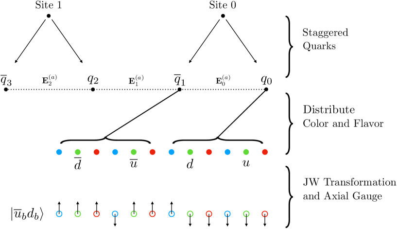
Figure 1: The encoding of $N_{f}=2$ QCD onto a lattice of spins describing $L=2$ spatial sites. Staggering is used to discretize the quark fields, which doubles the number of lattice sites, with (anti)quarks on (odd) even sites. The chromo-electric field resides on the links between quarks and antiquarks. Color and flavor degrees of freedom of each quark and antiquark site are distributed over six qubits with a JW mapping, and axial gauge along with Gauss’s law are used to remove the chromo-electric fields. A quark (antiquark) site is occupied if it is spin up (down), and the example spin configuration corresponds to the state $\ket{\overline{u}_{b}\,d_{b}}$.

The resulting JW-mapped Hamiltonian is the sum of the following five terms:

$$H= \ H_{kin}\ +\ H_{m}\ +\ H_{el}\ +\ H_{\mu_{B}}\ +\ H_{\mu_{I}}\ ,$$ (6a)

$$H_{kin}= \ -\frac{1}{2}\sum_{n=0}^{2L-2}\sum_{f=0}^{1}\sum_{c=0}^{2}\left[\sigma^{+}_{6n+3f+c}\left(\bigotimes_{i=1}^{5}\sigma^{z}_{6n+3f+c+i}\right)\sigma^{-}_{6(n+1)+3f+c}+\rm{h.c.}\right]\ ,$$ (6b)

$$H_{m}= \ \frac{1}{2}\sum_{n=0}^{2L-1}\sum_{f=0}^{1}\sum_{c=0}^{2}m_{f}\left[(-1)^{n}\sigma_{6n+3f+c}^{z}+1\right]\ ,$$ (6c)

$$H_{el}= \ \frac{g^{2}}{2}\sum_{n=0}^{2L-2}(2L-1-n)\left(\sum_{f=0}^{1}Q_{n,f}^{(a)}\,Q_{n,f}^{(a)}\ +\ 2Q_{n,0}^{(a)}\,Q_{n,1}^{(a)}\right)$$

$$+g^{2}\sum_{n=0}^{2L-3}\sum_{m=n+1}^{2L-2}(2L-1-m)\sum_{f=0}^{1}\sum_{f^{\prime}=0}^{1}Q_{n,f}^{(a)}\,Q_{m,f^{\prime}}^{(a)}\ ,$$ (6d)

$$H_{\mu_{B}}= \ -\frac{\mu_{B}}{6}\sum_{n=0}^{2L-1}\sum_{f=0}^{1}\sum_{c=0}^{2}\sigma_{6n+3f+c}^{z}\ ,$$ (6e)

$$H_{\mu_{I}}= \ -\frac{\mu_{I}}{4}\sum_{n=0}^{2L-1}\sum_{f=0}^{1}\sum_{c=0}^{2}(-1)^{f}\sigma_{6n+3f+c}^{z}\ ,$$ (6f)

where now repeated adjoint color indices, $(a)$, are summed over, the flavor indices, $f=0,1$, correspond to $u$- and $d$-quark flavors and $\sigma^{\pm}=(\sigma^{x}\pm i\sigma^{y})/2$. Products of charges are given in terms of spin operators as

$$Q_{n,f}^{(a)}\,Q_{n,f}^{(a)}= \frac{1}{3}(3-\sigma^{z}_{6n+3f}\sigma^{z}_{6n+3f+1}-\sigma^{z}_{6n+3f}\sigma^{z}_{6n+3f+2}-\sigma^{z}_{6n+3f+1}\sigma^{z}_{6n+3f+2})\ ,$$

$$Q_{n,f}^{(a)}\,Q_{m,f^{\prime}}^{(a)}= \frac{1}{4}\bigg{[}2\big{(}\sigma^{+}_{6n+3f}\sigma^{-}_{6n+3f+1}\sigma^{-}_{6m+3f^{\prime}}\sigma^{+}_{6m+3f^{\prime}+1}+\sigma^{+}_{6n+3f}\sigma^{z}_{6n+3f+1}\sigma^{-}_{6n+3f+2}\sigma^{-}_{6m+3f^{\prime}}\sigma^{z}_{6m+3f^{\prime}+1}\sigma^{+}_{6m+3f^{\prime}+2}$$

$$+\sigma^{+}_{6n+3f+1}\sigma^{-}_{6n+3f+2}\sigma^{-}_{6m+3f^{\prime}+1}\sigma^{+}_{6m+3f^{\prime}+2}+{\rm h.c.}\big{)}+\frac{1}{6}\sum_{c=0}^{2}\sum_{c^{\prime}=0}^{2}(3\delta_{cc^{\prime}}-1)\sigma^{z}_{6n+3f+c}\sigma^{z}_{6m+3f^{\prime}+c^{\prime}}\bigg{]}\ .$$ (7)

A constant has been added to $H_{m}$ to ensure that all basis states contribute positive mass. The Hamiltonian for $SU(N_{c})$ gauge theory with $N_{f}$ flavors in the fundamental representation is presented in Sec. IV. Note that choosing $A^{(a)}_{x}=0$ gauge and enforcing Gauss’s law has resulted in all-to-all interactions, the double lattice sum in $H_{el}$.

For any finite lattice system, there are color non-singlet states in the spectrum, which are unphysical and have infinite energy in the continuum and infinite-volume limits. For a large but finite system, OBCs can also support finite-energy color non-singlet states which are localized to the end of the lattice (color edge-states). The existence of such states in the spectrum is independent of the choice of gauge or fermion mapping. The naive ways to systematically examine basis states and preclude such configurations is found to be impractical due to the non-Abelian nature of the gauge charges and the resulting entanglement between states required for color neutrality. A practical way to deal with this problem is to add a term to the Hamiltonian that raises the energy of color non-singlet states. This can be accomplished by including the energy density in the chromo-electric field beyond the end of the lattice with a large coefficient $h$. This effectively adds the energy density in a finite chromo-electric field over a large spatial extent beyond the end of the lattice. In the limit $h\rightarrow\infty$, only states with a vanishing chromo-electric field beyond the end of the lattice remain at finite energy, rendering the system within the lattice to be a color singlet. This new term in the Hamiltonian is

$$H_{\bf 1}=\frac{h^{2}}{2}\sum_{n=0}^{2L-1}\left(\sum_{f=0}^{1}Q_{n,f}^{(a)}\,Q_{n,f}^{(a)}\ +\ 2Q_{n,0}^{(a)}\,Q_{n,1}^{(a)}\right)\ +\ h^{2}\sum_{n=0}^{2L-2}\sum_{m=n+1}^{2L-1}\sum_{f=0}^{1}\sum_{f^{\prime}=0}^{1}Q_{n,f}^{(a)}\,Q_{m,f^{\prime}}^{(a)}\ ,$$ (8)

which makes a vanishing contribution when the sum of charges over the whole lattice is zero; otherwise, it makes a contribution $\sim h^{2}$.

II.2 Spectra for $L=1,2$ Spatial Sites

The spectra and wavefunctions of systems with a small number of lattice sites can be determined by diagonalization of the Hamiltonian. In terms of spin operators, the $N_{f}=2$ Hamiltonian in Eq. (6) decomposes into sums of tensor products of Pauli matrices. The tensor product factorization can be exploited to perform an exact diagonalization relatively efficiently. This is accomplished by first constructing a basis by projecting onto states with specific quantum numbers, and then building the Hamiltonian in that subspace. There are four mutually commuting symmetry generators that allow states to be labelled by $(r,g,b,I_{3})$: redness, greenness, blueness and the third component of isospin. In the computational (occupation) basis, states are represented by bit strings of $0$s and $1$s. For example, the $L=1$ state with no occupation is $\ket{000000111111}$. Projecting onto eigenstates of $(r,g,b,I_{3})$ amounts to fixing the total number of $1$s in a substring of a state. The Hamiltonian is formed by evaluating matrix elements of Pauli strings between states in the basis, and only involves $2\times 2$ matrix multiplication. The Hamiltonian matrix is found to be sparse, as expected, and the low energy eigenvalues and eigenstates can be found straightforwardly. As the dimension of the Hamiltonian grows exponentially with the spatial extent of the lattice, this method becomes intractable for large system sizes, as is well known.

II.2.1 Exact Diagonalizations, Color Edge-States and Mass Decompositions of the Hadrons

For small enough systems, an exact diagonalization of the Hamiltonian matrix in the previously described basis can be performed. Without chiral symmetry and its spontaneous breaking, the energy spectrum in $1+1$D does not contain a massless isovector state (corresponding to the QCD pion) in the limit of vanishing quark masses. In the absence of chemical potentials for baryon number, $\mu_{B}=0$, or isospin, $\mu_{I}=0$, the vacuum, $\ket{\Omega}$, has $B=0$ (baryon number zero) and $I=0$ (zero total isospin). The $I=0$ $\sigma$-meson is the lightest meson, while the $I=1$ $\pi$-meson is the next lightest. The lowest-lying eigenstates in the $B=0$ spectra for $L=1,2$ (obtained from exact diagonalization of the Hamiltonian) are given in Table 1. The masses are defined by their energy gap to the vacuum, and all results in this section are for $m_{u}=m_{d}=m=1$.

$L=1$
$g^{2}$	$E_{\Omega}$	$M_{\sigma}$	$M_{\pi}$
8	-0.205	5.73	5.82
4	-0.321	4.37	4.47
2	-0.445	3.26	3.30
1	-0.549	2.73	2.74
1/2	-0.619	2.48	2.48
1/4	-0.661	2.35	2.36
1/8	-0.684	2.29	2.30

$L=2$
$g^{2}$	$E_{\Omega}$	$M_{\sigma}$	$M_{\pi}$
8	-0.611	5.82	5.92
4	-0.949	4.41	4.49
2	-1.30	3.27	3.31
1	-1.58	2.72	2.74
1/2	-1.77	2.45	2.46
1/4	-1.88	2.30	2.31
1/8	-1.94	2.22	2.22

Table 1: The vacuum energy and the masses of the $\sigma$- and $\pi$-mesons for $1+1$D QCD with $N_{f}=2$ for systems with $L=1,2$ spatial sites. These results are insensitive to $h$ as they are color singlets.

By examining the vacuum energy density $E_{\Omega}/L$, it is clear that, as expected, this number of lattice sites is insufficient to fully contain hadronic correlation lengths. While Table 1 shows the energies of color-singlet states, there are also non-singlet states in the spectra with similar masses, which become increasingly localized near the end of the lattice, as discussed in the previous section.

It is informative to examine the spectrum of the $L=1$ system as both $g$ and $h$ are slowly increased and, in particular, take note of the relevant symmetries. For $g=h=0$, with contributions from only the hopping and mass terms, the system exhibits a global $SU(12)$ symmetry where the spectrum is that of free quasi-particles; see App. B. The enhanced global symmetry at this special point restricts the structure of the spectrum to the ${\bf 1}$ and ${\bf 12}$ of $SU(12)$ as well as the antisymmetric combinations of fundamental irreps, ${\bf 66},{\bf 220},\ldots$. For $g>0$, these $SU(12)$ irreps split into irreps of color $SU(3)_{c}$ and flavor $SU(2)_{f}$. The ${\bf 12}$ corresponds to single quark ($q$) or antiquark ($\overline{q}$) excitations (with fractional baryon number), and splits into ${\bf 3}_{c}\otimes{\bf 2}_{f}$ for quarks and $\overline{\bf 3}_{c}\otimes{\bf 2}_{f}$ for antiquarks. In the absence of OBCs, these states would remain degenerate, but the boundary condition of vanishing background chromo-electric field is not invariant under $q\leftrightarrow\overline{q}$ and the quarks get pushed to higher mass. As there is no chromo-electric energy associated with exciting an antiquark at the end of the lattice in this mapping, the $\overline{\bf 3}_{c}\otimes{\bf 2}_{f}$ states remains low in the spectrum until $h\gg 0$. The ${\bf 66}$ corresponds to two-particle excitations, and contains all combinations of $qq$, $\overline{q}q$ and $\overline{q}\overline{q}$ excitations. The mixed color symmetry (i.e., neither symmetric or antisymmetric) of $\overline{q}q$ excitations allows for states with ${\bf 1}_{c}\otimes{\bf 1}_{f}\oplus{\bf 1}_{c}\otimes{\bf 3}_{f}\oplus{\bf 8}_{c}\otimes{\bf 1}_{f}\oplus{\bf 8}_{c}\otimes{\bf 3}_{f}$, while the $qq$ excitations with definite color symmetry allow for ${\bf 6}_{c}\otimes{\bf 1}_{f}\oplus\overline{\bf 3}_{c}\otimes{\bf 3}_{f}$ and $\overline{q}\overline{q}$ excitations allow for $\overline{\bf 6}_{c}\otimes{\bf 1}_{f}\oplus{\bf 3}_{c}\otimes{\bf 3}_{f}$, saturating the $66$ states in the multiplet. When $g>0$, these different configurations split in energy, and when $h\gg 0$, only color-singlet states are left in the low-lying spectrum. Figure 2 shows the evolution of the spectrum as $g$ and $h$ increase. The increase in mass of non-singlet color states with $h$ is proportional to the Casimir of the $SU(3)_{c}$ representation which is evident in Fig. 2 where, for example, the increase in the mass of the ${\bf 3}_{c}$s and $\overline{{\bf 3}}_{c}$s between $h^{2}=0$ and $h^{2}=0.64$ are the same.

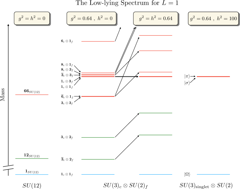
Figure 2: The spectrum of the Hamiltonian as the couplings $g$ and $h$ increase. For $g=h=0$ there is an exact $SU(12)$ symmetry and the color-singlet $\sigma$- and $\pi$-mesons are a part of the antisymmetric ${\bf 66}$ irrep. When $g>0$ and $h=0$, the spectrum splits into irreps of global $SU(3)_{c}\otimes SU(2)_{f}$ with color non-singlet states among the low-lying states. Increasing $h>0$ pushes non-singlet color states out of the low-lying spectrum. Notice that the $\sigma$ and $\pi$ masses are insensitive to $h$, as expected.

The antiquark states are particularly interesting as they correspond to edge states that are not “penalized” in energy by the chromo-electric field when $h=0$. These states have an approximate $SU(6)$ symmetry where the $6$ antiquarks transform in the fundamental. This is evident in the spectrum shown in Fig. 3 by the presence of a $\overline{{\bf 3}}_{c}\otimes{\bf 2}_{f}$ and nearly degenerate $\overline{\bf 6}_{c}\otimes{\bf 1}_{f}$ and ${\bf 3}_{c}\otimes{\bf 3}_{f}$ which are identified as states of a ${\bf 15}$ (an antisymmetric irrep of $SU(6)$) that do not increase in mass as $g$ increases. This edge-state $SU(6)$ symmetry is not exact due to interactions from the hopping term that couple the edge $\overline{q}$s to the rest of the lattice. These colored edge states are artifacts of OBCs and will persist in the low-lying spectrum for larger lattices.

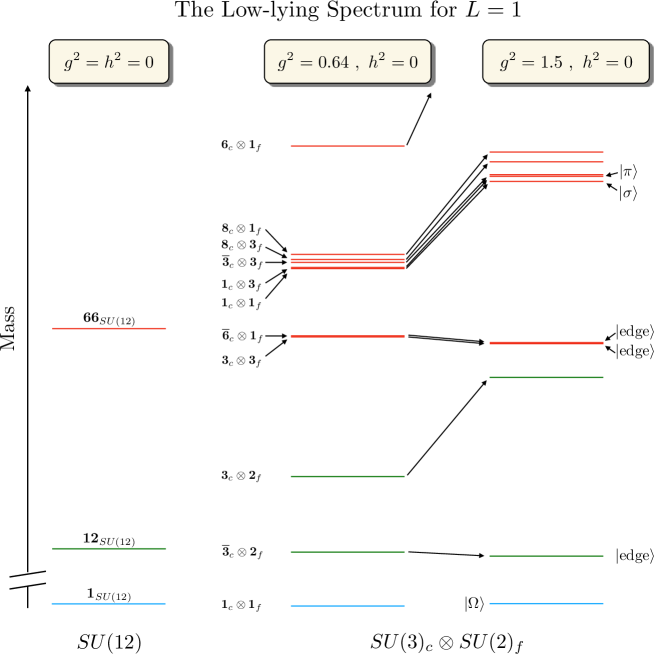
Figure 3: The spectrum of the Hamiltonian as $g$ increases for $h=0$. When $g=h=0$ there is an exact $SU(12)$ symmetry and the $\sigma$- and $\pi$-mesons are a part of the antisymmetric ${\bf 66}$ irrep. When $g>0$ but $h=0$ the spectrum splits into irreps of global $SU(3)_{c}\otimes SU(2)_{f}$, and non-singlet color states remain in the low-lying spectrum. Increasing $g$ shifts all but the antiquark $\ket{\text{edge}}$ (states) to higher mass.

Figures 2 and 3 reveal the near-degeneracy of the $\sigma$- and $\pi$-mesons throughout the range of couplings $g$ and $h$, suggesting another approximate symmetry, which can be understood in the small and large $g$ limits. For small $g^{2}$, the effect of $H_{el}=\frac{g^{2}}{2}(Q_{0,u}^{(a)}+Q_{0,d}^{(a)})^{2}$ on the the $SU(12)$-symmetric spectrum can be obtained through perturbation theory. To first order in $g^{2}$, the shift in the energy of any state is equal to the expectation value of $H_{el}$. The $\sigma$- and $\pi$-meson states are both quark-antiquark states in the 66 irrep of $SU(12)$, and therefore, both have a ${\bf 3}_{c}$ color charge on the quark site and receive the same mass shift. For large $g^{2}$, the only finite-energy excitations of the trivial vacuum (all sites unoccupied) are bare baryons and antibaryons, and the spectrum is one of non-interacting color-singlet baryons. Each quark (antiquark) site hosts $4$ distinct baryons (antibaryons) in correspondence with the multiplicity of the $I=3/2$ irrep. As a result, the $\sigma$, $\pi$, $I=2,3$ mesons, deuteron and antideuteron are all degenerate.

The $\sigma$- and $\pi$-meson mass splitting is shown in Fig. 4 and has a clear maxima for $g\sim 2.4$. Intriguingly, this corresponds to the maximum of the linear entropy between quark and antiquarks (as discussed in Sec. II.2.3), and suggests a connection between symmetry, via degeneracies in the spectrum, and entanglement. This shares similarities with the correspondence between Wigner’s $SU(4)$ spin-flavor symmetry [148, 149, 150], which becomes manifest in low-energy nuclear forces in the large-$N_{c}$ limit of QCD [151, 152], and entanglement suppression in nucleon-nucleon scattering found in Ref. [153] (see also Refs. [154, 155, 156]).

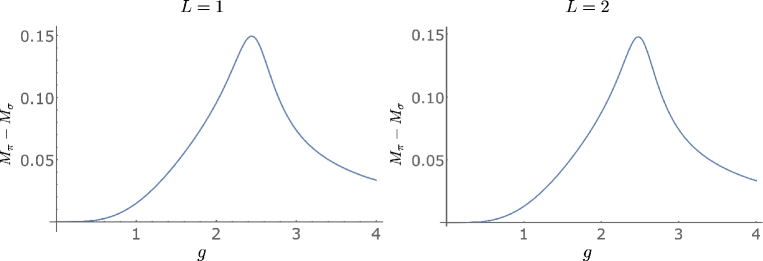
Figure 4: The mass splitting between the $\sigma$- and $\pi$-mesons for $L=1$ (left panel) and $L=2$ (right panel).

Color singlet baryons are also present in this system, formed by contracting the color indices of three quarks with a Levi-Civita tensor (and antibaryons are formed from three antiquarks). A baryon is composed of three $I=1/2$ quarks in the (symmetric) $I=3/2$ configuration and in a (antisymmetric) color singlet. It will be referred to as the $\Delta$, highlighting its similarity to the $\Delta$-resonance in $3+1$D QCD. Interestingly, there is an isoscalar $\Delta\Delta$ bound state, which will be referred to as the deuteron. The existence of a deuteron makes this system valuable from the standpoint of quantum simulations of the formation of nuclei in a model of reduced complexity. The mass of the $\Delta$, $M_{\Delta}$, and the binding energy of the deuteron, $B_{\Delta\Delta}=2M_{\Delta}-M_{\Delta\Delta}$, are shown in Table 2 for a range of strong couplings.

$L=1$
$g^{2}$	$M_{\Delta}$	$B_{\Delta\Delta}$
8	3.10	$2.61\times 10^{-4}$
4	3.16	$5.48\times 10^{-4}$
2	3.22	$6.12\times 10^{-4}$
1	3.27	$3.84\times 10^{-4}$
1/2	3.31	$1.61\times 10^{-4}$
1/4	3.33	$5.27\times 10^{-5}$
1/8	3.34	$1.52\times 10^{-5}$

$L=2$
$g^{2}$	$M_{\Delta}$	$B_{\Delta\Delta}$
8	3.10	$2.50\times 10^{-4}$
4	3.16	$4.95\times 10^{-4}$
2	3.21	$5.07\times 10^{-4}$
1	3.24	$4.60\times 10^{-4}$
1/2	3.25	$1.53\times 10^{-3}$
1/4	3.23	$3.91\times 10^{-3}$
1/8	3.20	$3.35\times 10^{-3}$

Table 2: The mass of the $\Delta$ and the binding energy of the deuteron in $1+1$D QCD with $N_{f}=2$ for systems with $L=1,2$ spatial sites.

Understanding and quantifying the structure of the lowest-lying hadrons is a priority for nuclear physics research [157]. Great progress has been made, experimentally, analytically and computationally, in dissecting the mass and angular momentum of the proton (see, for example, Refs. [158, 159, 160, 161, 162, 163, 164, 165]). This provides, in part, the foundation for anticipated precision studies at the future electron-ion collider (EIC) [166, 167] at Brookhaven National Laboratory. Decompositions of the vacuum energy and the masses of the $\sigma$, $\pi$ and $\Delta$ are shown in Fig. 5 where, for example, the chromo-electric contribution to the $\sigma$ is $\langle H_{el}\rangle=\bra{\sigma}H_{el}\ket{\sigma}-\bra{\Omega}H_{el}\ket{\Omega}$. These calculations demonstrate the potential of future quantum simulations in being able to quantify decompositions of properties of the nucleon, including in dense matter. For the baryon states, it is $H_{el}$ that is responsible for the system coalescing into localized color singlets in order to minimize the energy in the chromo-electric field (between spatial sites).

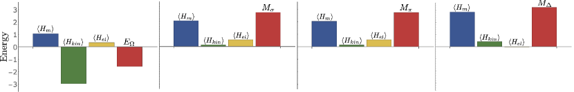
Figure 5: The decomposition of vacuum energy ($E_{\Omega}$) and the masses of the lightest hadrons ($M_{\sigma}$, $M_{\pi}$ and $M_{\Delta}$) into contributions from the mass, the kinetic and the chromo-electric field terms in the Hamiltonian, defined in axial gauge, for $1+1$D QCD with $N_{f}=L=2$ and $m=g=1$.

The deuteron binding energy is shown in the left panel of Fig. 6 as a function of $g$. While the deuteron is unbound at $g=0$ for obvious reasons, it is also unbound at large $g$ because the spectrum is that of non-interacting color-singlet (anti)baryons. Therefore, the non-trivial aspects of deuteron binding for these systems is for intermediate values of $g$. The decomposition of $B_{\Delta\Delta}$ is shown in the right panel of Fig. 6, where, for example, the chromo-electric contribution is

$$\langle H_{el}\rangle=2\big{(}\bra{\Delta}H_{el}\ket{\Delta}-\bra{\Omega}H_{el}\ket{\Omega}\big{)}-\big{(}\bra{\Delta\Delta}H_{el}\ket{\Delta\Delta}-\bra{\Omega}H_{el}\ket{\Omega}\big{)}\ .$$ (9)

The largest contribution to the binding energy is $\langle H_{kin}\rangle$, which is the term responsible for creating $q\overline{q}$ pairs. This suggests that meson-exchange may play a significant role in the attraction between baryons, as is the case in $3+1$D QCD, but larger systems will need to be studied before definitive conclusions can be drawn. One consequence of the lightest baryon being $I=3/2$ is that, for $L=1$, the $I_{3}=+3/2$ state completely occupies the up-quark sites. Thus the system factorizes into an inert up-quark sector and a dynamic down-quark sector, and the absolute energy of the lowest-lying baryon state can be written as $E_{\Delta}=M_{\Delta}+E_{\Omega}^{2f}=3m+E_{\Omega}^{1f}$, where $E_{\Omega}^{1,2f}$ is the vacuum energy of the $N_{f}=1,2$ flavor systems. Analogously, the deuteron absolute energy is $E_{\Delta\Delta}=6m$, and therefore the deuteron binding energy can be written as $B_{\Delta\Delta}=2(3m+E_{\Omega}^{1f}-E_{\Omega}^{2f})-(6m-E_{\Omega}^{2f})=2E_{\Omega}^{1f}-E_{\Omega}^{2f}$. This is quite a remarkable result because, in this system, the deuteron binding energy depends only on the difference between the $N_{f}=1$ and $N_{f}=2$ vacuum energies, being bound when $2E_{\Omega}^{1f}-E_{\Omega}^{2f}>0$. As has been discussed previously, it is the $q\overline{q}$ contribution from this difference that dominates the binding.

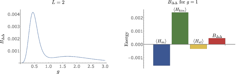
Figure 6: The left panel shows the deuteron binding energy, $B_{\Delta\Delta}$, for $m=1$ and $L=2$. The right panel shows the decomposition of $B_{\Delta\Delta}$ into contributions from the Hamiltonian for $g=1$.

II.2.2 The Low-Lying Spectrum Using D-Wave’s Quantum Annealers

The low-lying spectrum of this system can also be determined through annealing by using D-Wave’s quantum annealer (QA) Advantage [168], a device with 5627 superconducting flux qubits, with a 15-way qubit connectivity via Josephson junctions rf-SQUID couplers [169]. Not only did this enable the determination of the energies of low-lying states, but it also assessed the ability of this quantum device to isolate nearly degenerate states. The time-dependent Hamiltonian of the device, which our systems are to be mapped, are of the form of an Ising model, with the freedom to specify the single- and two-qubit coefficients. Alternatively, the Ising model can be rewritten in a quadratic unconstrained binary optimization (QUBO) form, $f_{Q}(x)=\sum_{ij}Q_{ij}x_{i}x_{j}$, where $x_{i}$ are binary variables and $Q_{ij}$ is a QUBO matrix, which contains the coefficients of single-qubit ($i=j$) and two-qubit ($i\neq j$) terms. The QUBO matrix is the input that is submitted to Advantage, with the output being a bit-string that minimizes $f_{Q}$. Due to the qubit connectivity of Advantage, multiple physical qubits are chained together to recover the required connectivity, limiting the system size that can be annealed.

The QA Advantage was used to determine the lowest three states in the $B=0$ sector of the $L=1$ system, with $m=g=1$ and $h=2$, following techniques presented in Ref. [74]. In that work, the objective function to be minimized is defined as $F=\langle\Psi\rvert\tilde{H}\lvert\Psi\rangle-\eta\langle\Psi|\Psi\rangle$ [170], where $\eta$ is a parameter that is included to avoid the null solution, and its optimal value can be iteratively tuned to be as close to the ground-state energy as possible. The wavefunction is expanded in a finite dimensional orthonormal basis $\psi_{\alpha}$, $\lvert\Psi\rangle=\sum^{n_{s}}_{\alpha}a_{\alpha}|\psi_{\alpha}\rangle$, which in this case reduces the dimensionality of $H$ to $88$, defining $\tilde{H}$, thus making it feasible to study with Advantage. The procedure to write the objective function in a QUBO form can be found in Ref. [74] (and briefly described in App. C), where the coefficients $a_{\alpha}$ are digitized using $K$ binary variables [170], and the adaptive QA eigenvalue solver is implemented by using the zooming method [171, 57]. To reduce the uncertainty in the resulting energy and wavefunction, due to the noisy nature of this QA, the iterative procedure described in Ref. [74] was used, where the (low-precision) solution obtained from the machine after several zooming steps constituted the starting point of a new anneal. This led to a reduction of the uncertainty by an order of magnitude (while effectively only doubling the resources used).

Results obtained using Advantage are shown in Fig. 7, where the three panels show the convergence of the energy of the vacuum state (left), the mass of the $\sigma$-meson (center) and the mass of the $\pi$-meson (right) as a function of zoom steps, as well as comparisons to the exact wavefunctions. The bands in the plot correspond to 68% confidence intervals determined from 20 independent runs of the annealing workflow, where each corresponds to $10^{3}$ anneals with an annealing time of $t_{A}=20$ $\mu$s, and the points correspond to the lowest energy found by the QA. The parameter $K$ in the digitization of $a_{\alpha}$ is set to $K=2$. The parameter $\eta$ is first set close enough to the corresponding energy (e.g., $\eta=0$ for the ground-state), and for the subsequent iterative steps it is set to the lowest energy found in the previous step. The first two excited states are nearly degenerate, and after projecting out the ground state, Advantage finds both states in the first step of the iterative procedure (as shown by the yellow lines in the $\pi$ wavefunction of Fig. 7). However, after one iterative step, the QA converges to one of the two excited states. It first finds the second excited state (the $\pi$-meson), and once this state is known with sufficient precision, it can be projected out to study the other excited state. The converged values for the energies and masses of these states are shown in Table 3, along with the exact results. The uncertainties in these values should be understood as uncertainties on an upper bound of the energy (as they result from a variational calculation). For more details see App. C.

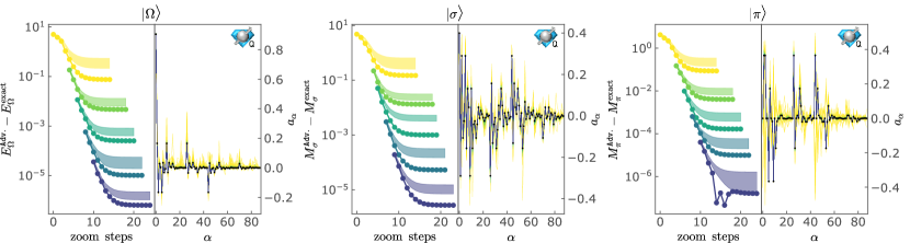
Figure 7: Iterative convergence of the energy, masses and wavefunctions for the three lowest-lying states in the $B=0$ sector of $1+1$D QCD with $N_{f}=2$ and $m=g=L=1$: vacuum (left), $\sigma$-meson (center) and $\pi$-meson (right). The different colors correspond to different steps of the iterative procedure that is described in the main text. The oscillatory behavior seen in the right panel around the 15th zoom step is discussed in App. C. The blue icons in the upper right indicate that this calculation was done on a quantum device [38].

$L=1$
		$\ket{\Omega}$	$\ket{\sigma}$	$\ket{\pi}$
Exact	Energy	$-0.5491067$	$2.177749$	$2.1926786$
	Mass	-	$2.726855$	$2.7417853$
Advantage	Energy	$-0.5491051(6)$	$2.177760(4)$	$2.1926809(7)$
	Mass	-	$2.726865(4)$	$2.7417860(9)$

Table 3: Energies and masses of the three lowest-lying states in the $B=0$ sector of $1+1$D QCD with $N_{f}=2$ and $m=g=L=1$. Shown are the exact results from diagonalization of the Hamiltonian matrix and those obtained from D-Wave’s Advantage.

II.2.3 Quark-Antiquark Entanglement in the Spectra via Exact Diagonalization

With $h\gg g$, the eigenstates of the Hamiltonian are color singlets and irreps of isospin. As these are global quantum numbers (summed over the lattice) the eigenstates are generically entangled among the color and isospin components at each lattice site. With the hope of gaining insight into $3+1$D QCD, aspects of the entanglement structure of the $L=1$ wavefunctions are explored via exact methods. An interesting measure of entanglement for these systems is the linear entropy between quarks and antiquarks, defined as

$$S_{L}=1-\Tr[\rho_{q}^{2}]\ ,$$ (10)

where $\rho_{q}=\Tr_{\overline{q}}[\rho]$ and $\rho$ is a density matrix of the system. Shown in Fig. 8 is the linear entropy between quarks and antiquarks in $\ket{\Omega}$, $\ket{\sigma}$, $\ket{\pi_{I_{3}=1}}$ and $\ket{\Delta_{I_{3}=3/2}}$ as a function of $g$.

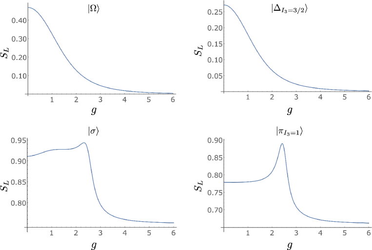
Figure 8: The linear entropy between quarks and antiquarks in $\ket{\Omega}$, $\ket{\Delta_{I_{3}=3/2}}$, $\ket{\sigma}$ and $\ket{\pi_{I_{3}=1}}$ for $m=L=1$.

The deuteron is not shown as there is only one basis state contributing for $L=1$.

The scaling of the linear entropy in the vacuum and baryon with $g$ can be understood as follows. As $g$ increases, color singlets on each site have the least energy density. The vacuum becomes dominated by the unoccupied state and the $\Delta$ becomes dominated by the “bare” $\Delta$ with all three quarks located on one site in a color singlet. As the entropy generically scales with the number of available states, the vacuum and baryon have decreasing entropy for increasing $g$. The situation for the $\pi$ and $\sigma$ is somewhat more interesting. For small $g$, their wavefunctions are dominated by $q\overline{q}$ excitations on top of the trivial vacuum, which minimizes the contributions from the mass term. However, color singlets are preferred as $g$ increases, and the mesons become primarily composed of baryon-antibaryon ($B\overline{B}$) excitations. There are more $q\overline{q}$ states than $B\overline{B}$ states with a given $I_{3}$, and therefore there is more entropy at small $g$ than large $g$. The peak at intermediate $g$ occurs at the crossover between these two regimes where the meson has a sizable contribution from both $q\overline{q}$ and $B\overline{B}$ excitations. To illustrate this, the expectation value of total quark occupation (number of quarks plus the number of antiquarks) is shown in Fig. 9. For small $g$, the occupation is near $2$ since the state is mostly composed of $q\overline{q}$, while for large $g$ it approaches $6$ as the state mostly consists of $B\overline{B}$. This is a transition from the excitations being “color-flux tubes” between quark and antiquark of the same color to bound states of color-singlet baryons and antibaryons.

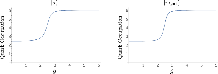
Figure 9: The expectation value of quark occupation in the $\ket{\sigma}$ and $\ket{\pi_{I_{3}=1}}$ for $m=L=1$.

II.3 Digital Quantum Circuits

The Hamiltonian for $1+1$D QCD with arbitrary $N_{c}$ and $N_{f}$, when written in terms of spin operators, can be naturally mapped onto a quantum device with qubit registers. In this section the time evolution for systems with $N_{c}=3$ and $N_{f}=2$ are developed.

II.3.1 Time Evolution

To perform time evolution on a quantum computer, the operator $U(t)=\exp(-iHt)$ is reproduced by a sequence of gates applied to the qubit register. Generally, a Hamiltonian cannot be directly mapped to such a sequence efficiently, but each of the elements in a Trotter decomposition can, with systematically reducible errors. Typically, the Hamiltonian is divided into Pauli strings whose unitary evolution can be implemented with quantum circuits that are readily constructed. For a Trotter step of size $t$, the circuit that implements the time evolution from the mass term, $U_{m}(t)=\exp(-iH_{m}t)$, is shown in Fig. 10.

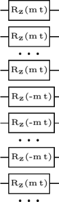
Figure 10: The quantum circuit that implements time evolution by the mass term, $U_{m}(t)=\exp(-iH_{m}t)$.

The staggered mass leads to quarks being rotated by a positive angle and antiquarks being rotated by a negative angle. Only single qubit rotations about the z-axis are required for its implementation, with $R_{Z}(\theta)=\exp(-i\theta Z/2)$. The circuit that implements the evolution from the baryon chemical potential, $\mu_{B}$, $U_{\mu_{B}}(t)=\exp(-iH_{\mu_{B}}t)$, is similar to $U_{m}(t)$ with $m\to\mu_{B}/3$, and with both quarks and antiquarks rotated by the same angle. Similarly, the circuit that implements the evolution from the isospin chemical potential, $\mu_{I}$, $U_{\mu_{I}}(t)=\exp(-iH_{\mu_{I}}t)$, is similar to $U_{m}(t)$ with $m\to\mu_{I}/2$ and up (down) quarks rotated by a negative (positive) angle.

The kinetic piece of the Hamiltonian, Eq. (6b), is composed of hopping terms of the form

$$H_{kin}\ \sim\ \sigma^{+}ZZZZZ\sigma^{-}+\rm{h.c.}\ .$$ (11)

The $\sigma^{+}$ and $\sigma^{-}$ operators enable quarks and antiquarks to move between sites with the same color and flavor (create $\overline{q}^{\alpha}_{i}q_{\alpha}^{i}$ pairs) and the string of $Z$ operators incorporates the signs from Pauli statistics. The circuits for Trotterizing these terms are based on circuits in Ref. [172]. We introduce an ancilla to accumulate the parity of the JW string of $Z$s. This provides a mechanism for the different hopping terms to re-use previously computed (partial-)parity. The circuit for the first two hopping terms is shown in Fig. 11.

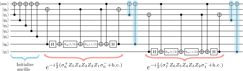
Figure 11: A circuit that implements the time evolution from two sequential hopping terms. Implementing $\exp(-iH_{kin}t)$ in Eq. (6b) is a straightforward extension of this circuit.

The first circuit operations initialize the ancilla to store the parity of the string of $Z$s between the first and last qubit of the string. Next, the system is evolved by the exponential of the hopping term. After the exponential of each hopping term, the ancilla is modified for the parity of the subsequent hopping term (the CNOTs highlighted in blue). Note that the hopping of quarks, or antiquarks, of different flavors and colors commute, and the Trotter decomposition is exact (without Trotterization errors) over a single spatial site.

Implementation of the time-evolution induced by the energy density in the chromo-electric field, $H_{el}$, given in Eq. (7), is the most challenging due to its inherent non-locality in axial gauge. There are two distinct types of contributions: One is from same-site interactions and the other from interactions between different sites. For the same-site interactions, the operator is the product of charges $Q_{n,f}^{(a)}\,Q_{n,f}^{(a)}$, which contains only $ZZ$ operators, and is digitized with the standard two CNOT circuit. The $Q_{n,f}^{(a)}\,Q_{m,f^{\prime}}^{(a)}$ operators contain 4-qubit interactions of the form $(\sigma^{+}\sigma^{-}\sigma^{-}\sigma^{+}+\ {\rm h.c.})$ and 6-qubit interactions of the form $(\sigma^{+}Z\sigma^{-}\sigma^{-}Z\sigma^{+}+\ {\rm h.c.})$, in addition to $ZZ$ contributions. The manipulations required to implement the 6-qubit operators parallel those required for the 4-qubit operators, and here only the latter is discussed in detail. These operators can be decomposed into eight mutually commuting terms,

$$\sigma^{+}\sigma^{-}\sigma^{-}\sigma^{+}+{\rm h.c.}=\frac{1}{8}(XXXX+YYXX+YXYX-YXXY-XYYX+XYXY+XXYY+YYYY)\ .$$ (12)

The strategy for identifying the corresponding time evolution circuit is to first apply a unitary that diagonalizes every term, apply the diagonal rotations, and finally, act with the inverse unitary to return to the computational basis. By only applying diagonal rotations, many of the CNOTs can be arranged to cancel. Each of the eight Pauli strings in Eq. (12) takes a state in the computational basis to the corresponding bit-flipped state (up to a phase). This suggests that the desired eigenbasis pairs together states with their bit-flipped counterpart, which is an inherent property of the GHZ basis [172]. In fact, any permutation of the GHZ state-preparation circuit diagonalizes the interaction. The two that will be used, denoted by $G$ and $\tilde{G}$, are shown in Fig. 12.

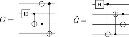
Figure 12: Two GHZ state-preparation circuits.

In the diagonal bases, the Pauli strings in Eq. (12) become

$$G^{\dagger}\ (\sigma^{+}\sigma^{-}\sigma^{-}\sigma^{+}+{\rm h.c.})\ G= \ \frac{1}{8}\left(IIZI-ZIZZ-ZZZZ+ZIZI+IZZI-IIZZ-IZZZ+ZZZI\right)\ ,$$

$$\tilde{G}^{\dagger}\ (\sigma^{+}\sigma^{-}\sigma^{-}\sigma^{+}+{\rm h.c.})\ \tilde{G}= \ \frac{1}{8}\left(IIIZ-IZZZ-IIZZ+ZIIZ+IZIZ-ZZZZ-ZIZZ+ZZIZ\right)\ .$$ (13)

Another simplification comes from the fact that $ZZ$ in the computational basis becomes a single $Z$ in a GHZ basis if the GHZ state-preparation circuit has a CNOT connecting the two $Z$s. For the case at hand, this implies

$$G^{\dagger}\ (IZZI+IZIZ+ZIIZ)\ G= \ IZII+IIIZ+ZIII\ ,$$

$$\tilde{G}^{\dagger}\ (ZIZI+IZZI+ZIIZ)\ \tilde{G}= \ IIZI+IZII+ZIII\ .$$ (14)

As a consequence, all nine $ZZ$ terms in $Q_{n,f}^{(a)}\,Q_{m,f^{\prime}}^{(a)}$ become single $Z$s in a GHZ basis, thus requiring no additional CNOT gates to implement. Central elements of the circuits required to implement time evolution of the chromo-electric energy density are shown in Fig. 13, which extends the circuit presented in Fig. 4 of Ref. [172] to non-Abelian gauge theories.

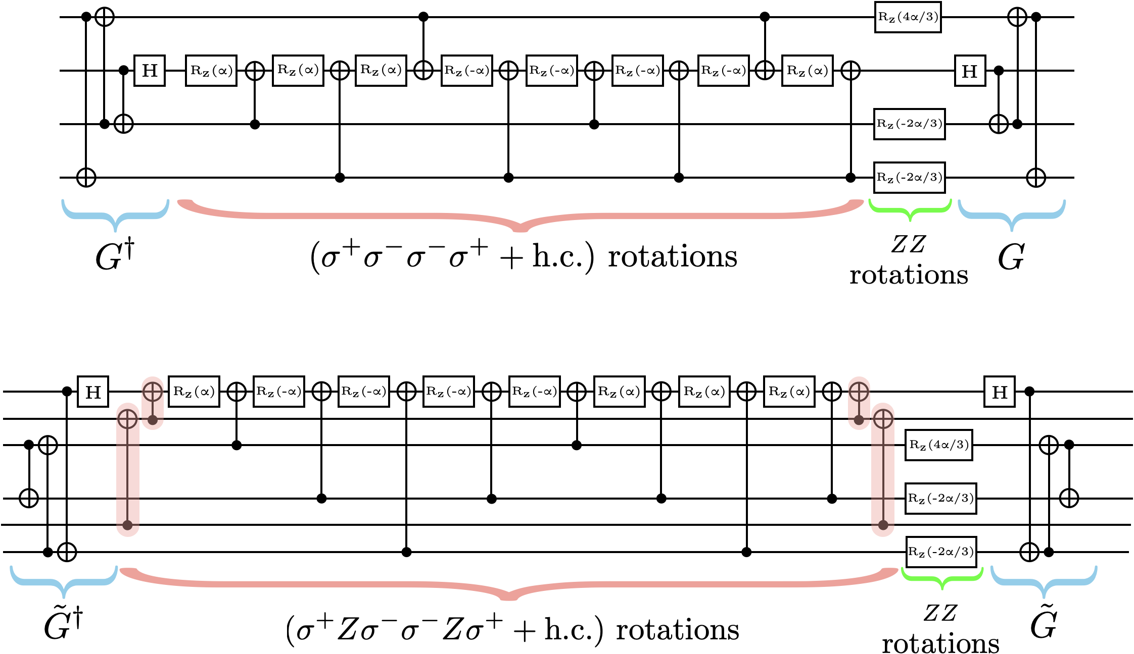
Figure 13: The circuits that implement the time evolution of ${\exp}(-8i\alpha Q_{n,f}^{(a)}\,Q_{m,f^{\prime}}^{(a)})$. Specifically, the upper circuit implements $\exp{-i4\alpha[(\sigma^{+}\sigma^{-}\sigma^{-}\sigma^{+}+{\rm h.c.})+\frac{1}{12}(2IZIZ-IZZI-ZIIZ)]}$, while the lower circuit implements $\exp{-i4\alpha[(\sigma^{+}Z\sigma^{-}\sigma^{-}Z\sigma^{-}+{\rm h.c.})+\frac{1}{12}(2ZIIZII-IIZZII-ZIIIIZ)]}$. The CNOTs highlighted in red account for the $Z$s in $\sigma^{+}Z\sigma^{-}\sigma^{-}Z\sigma^{+}$. For $SU(3)$ with $N_{f}=2$ and $L=1$, the required evolution operators have $\alpha=tg^{2}/8$.

More details on these circuits can be found in App. D.

II.3.2 Trotterization, Color Symmetry and Color Twirling

After fixing the gauge, the Hamiltonian is no longer manifestly invariant under local $SU(3)$ gauge transformations. However, as is well known, observables of the theory are correctly computed from such a gauge-fixed Hamiltonian, which possesses a remnant global $SU(3)$ symmetry. This section addresses the extent to which this symmetry is preserved by Trotterization of the time-evolution operator. The focus will be on the $N_{f}=1$ theory as including additional flavors does not introduce new complications.

Trotterization of the mass and kinetic parts of the Hamiltonian, while having non-zero commutators between some terms, preserves the global $SU(3)$ symmetry. The time evolution of $Q_{n}^{(a)}\,Q_{n}^{(a)}$ can be implemented in a unitary operator without Trotter errors, and, therefore, does not break $SU(3)$. On the other hand, the time evolution induced by $Q_{n}^{(a)}\,Q_{m}^{(a)}$ is implemented by the operator being divided into four terms: $(Q^{(1)}_{n}\,Q^{(1)}_{m}+Q^{(2)}_{n}\,Q^{(2)}_{m})$, $(Q^{(4)}_{n}\,Q^{(4)}_{m}+Q^{(5)}_{n}\,Q^{(5)}_{m})$, $(Q^{(6)}_{n}\,Q^{(6)}_{m}+Q^{(7)}_{n}\,Q^{(7)}_{m})$ and $(Q^{(3)}_{n}\,Q^{(3)}_{m}+Q^{(8)}_{n}\,Q^{(8)}_{m})$. In order for global $SU(3)$ to be unbroken, the sum over the entire lattice of each of the 8 gauge charges must be unchanged under time evolution. Therefore, the object of interest is the commutator

$$\mathcal{C}=\left[\sum_{n=0}^{2L-1}Q^{(a)}_{n}\ ,\ Q^{(\tilde{b})}_{m}\cdot Q^{(\tilde{b})}_{l}\right]\ ,$$ (15)

where $\tilde{b}$ is summed over the elements of one of the pairs in $\{(1,2),\,(4,5),\,(6,7),\,(3,8)\}$. It is found that this commutator only vanishes if $a=3$ or $a=8$, or if $\tilde{b}$ is summed over all $8$ values (as is the case for the exact time evolution operator). Therefore, Trotter time evolution does not preserve the global off-diagonal $SU(3)$ charges and, for example, color singlets can evolve into non-color singlets. Equivalently, the Trotterized time evolution operator is not in the trivial representation of $SU(3)$. To understand this point in more detail, consider the transformation of $\left(T^{a}\right)^{i}_{j}\ \left(T^{a}\right)^{k}_{l}$ for any given $a$. Because of the symmetry of this product of operators, each transforming as an ${\bf 8}$, the product must decompose into ${\bf 1}\oplus{\bf 8}\oplus{\bf 27}$, where the elements of each of the irreps can be found from

$$\left(T^{a}\right)^{i}_{j}\ \left(T^{a}\right)^{k}_{l}=\left(\hat{\cal O}_{27}^{a}\right)^{ik}_{jl}-\frac{2}{5}\left[\delta^{i}_{j}\left(\hat{\cal O}^{a}_{8}\right)^{k}_{l}+\delta^{k}_{l}\left(\hat{\cal O}^{a}_{8}\right)^{i}_{j}\right]+\frac{3}{5}\left[\delta^{i}_{l}\left(\hat{\cal O}^{a}_{8}\right)^{k}_{j}+\delta^{k}_{j}\left(\hat{\cal O}^{a}_{8}\right)^{i}_{l}\right]+\frac{1}{8}\left(\delta^{i}_{l}\delta^{k}_{j}\ -\ \frac{1}{3}\delta^{i}_{j}\delta^{k}_{l}\right)\hat{\cal O}^{a}_{1}\ ,$$ (16)

where

$$\left(\hat{\cal O}^{a}_{27}\right)^{ik}_{jl}= \ \frac{1}{2}\left[\left(T^{a}\right)^{i}_{j}\left(T^{a}\right)^{k}_{l}+\left(T^{a}\right)^{i}_{l}\left(T^{a}\right)^{k}_{j}\right]-\frac{1}{10}\left[\delta^{i}_{j}\left(\hat{\cal O}^{a}_{8}\right)^{k}_{l}+\delta^{i}_{l}\left(\hat{\cal O}^{a}_{8}\right)^{k}_{j}+\delta^{k}_{j}\left(\hat{\cal O}^{a}_{8}\right)^{i}_{l}+\delta^{k}_{l}\left(\hat{\cal O}^{a}_{8}\right)^{i}_{j}\right]$$

$$-\frac{1}{24}\left(\delta^{i}_{j}\delta^{k}_{l}+\delta^{i}_{l}\delta^{k}_{j}\right)\hat{\cal O}^{a}_{1}\ ,$$

$$\left(\hat{\cal O}^{a}_{8}\right)^{i}_{j}= \ \left(T^{a}\right)^{i}_{\beta}\left(T^{a}\right)_{j}^{\beta}\ -\ \frac{1}{3}\delta^{i}_{j}\hat{\cal O}^{a}_{1}\ ,\ \ \hat{\cal O}^{a}_{1}\ =\ \left(T^{a}\right)^{\alpha}_{\beta}\left(T^{a}\right)_{\alpha}^{\beta}\ =\ \frac{1}{2}\ .$$ (17)

When summed over $a=1,\ldots,8$, the contributions from the ${\bf 8}$ and ${\bf 27}$ vanish, leaving the familiar contribution from the ${\bf 1}$. When only partials sums are available, as is the situation with individual contributions to the Trotterized evolution, each of the contributions is the exponential of ${\bf 1}\oplus{\bf 8}\oplus{\bf 27}$, with only the singlet contributions leaving the lattice a color singlet. The leading term in the expansion of the product of the four pairs of Trotterized evolution operators sum to leave only the singlet contribution. In contrast, higher-order terms do not cancel and non-singlet contributions are present.

This is a generic problem that will be encountered when satisfying Gauss’s law leads to non-local charge-charge interactions. This is not a problem for $U(1)$, and surprisingly, is not a problem for $SU(2)$ because $(Q^{(1)}_{n}\,Q^{(1)}_{m},Q^{(2)}_{n}\,Q^{(2)}_{m},Q^{(3)}_{n}\,Q^{(3)}_{m})$ are in the Cartan sub-algebra of $SU(4)$ and therefore mutually commuting. However, it is a problem for $N_{c}>2$. One way around the breaking of global $SU(N_{c})$ is through the co-design of unitaries that directly (natively) implement ${\exp}(i\alpha Q^{(a)}_{n}\,Q^{(a)}_{m})$; see Sec. II.3.4. Without such a native unitary, the breaking of $SU(N_{c})$ appears as any other Trotter error, and can be systematically reduced in the same way. A potential caveat to this is if the time evolution operator took the system into a different phase, but our studies of $L=1$ show no evidence of this.

It is interesting to note that the terms generated by the Trotter commutators form a closed algebra. In principle, a finite number of terms could be included to define an effective Hamiltonian whose Trotterization exactly maps onto the desired evolution operator (without the extra terms). It is straightforward to work out the terms generated order-by-order in the Baker-Campbell-Hausdorff formula. Aside from re-normalizing the existing charges, there are $9$ new operator structures produced. For example, the leading-order commutators generate the three operators, ${\cal O}_{i}$, in Eq. (18),

$${\cal O}_{i}=\begin{cases}(\sigma^{+}I\sigma^{-}\sigma^{-}Z\sigma^{+}-\sigma^{+}Z\sigma^{-}\sigma^{-}I\sigma^{+})-{\rm h.c.}\ ,\\ (I\sigma^{-}\sigma^{+}Z\sigma^{+}\sigma^{-}-Z\sigma^{-}\sigma^{+}I\sigma^{+}\sigma^{-})-{\rm h.c.}\ ,\\ (\sigma^{+}\sigma^{-}Z\sigma^{-}\sigma^{+}I-\sigma^{+}\sigma^{-}I\sigma^{-}\sigma^{+}Z)-{\rm h.c.}\ .\end{cases}$$ (18)

In general, additional operators are constrained only by (anti)hermiticity, symmetry with respect to $n\leftrightarrow m$ and preservation of $(r,g,b)$, and should generically be included in the same spirit as terms in the Symanzik-action [175, 176] for lattice QCD.

With Trotterization of the gauge field introducing violations of gauge symmetry, and the presence of bit- and phase-flip errors within the device register, it is worth briefly considering a potential mitigation strategy. A single bit-flip error will change isospin by $|\Delta I_{3}|=1/2$ and color charge by one unit of red or green or blue. After each Trotter step on a real quantum device, such errors will be encountered and a mitigation or correction scheme is required. Without the explicit gauge-field degrees of freedom and local charge conservation checks enabled by Gauss’s law, such errors can only be detected globally, and hence, cannot be actively corrected during the evolution. Motivated by this, consider introducing a twirling phase factor into the evolution, $\exp(-i\theta^{a}{\cal Q}^{(a)})$, where ${\cal Q}^{(a)}$ is the total charge on the lattice. If applied after each Trotter step, with a randomly selected set of eight angles, $\theta^{a}$, the phases of color-nonsinglet states become random for each member of an ensemble, mitigating errors in some observables. Similar twirling phase factors could be included for the other charges that are conserved or approximately conserved.

II.3.3 Quantum Resource Requirements for Time Evolution

It is straightforward to extend the circuits presented in the previous section to arbitrary $N_{c}$ and $N_{f}$. The quantum resources required for time evolution can be quantified for small, modest and asymptotically large systems. As discussed previously, a quantum register with $N_{q}=2LN_{c}N_{f}$ qubits is required to encode one-dimensional $SU(N_{c})$ gauge theory with $N_{f}$ flavors on $L$ spatial lattice sites using the JW transformation. For $SU(3)$ gauge theory, this leads to, for example, $N_{q}=6L$ with only $u$-quarks and $N_{q}=18L$ with $u,d,s$-quarks. The five distinct contributions to the resource requirements, corresponding to application of the unitary operators providing a single Trotter step associated with the quark mass, $U_{m}$, the baryon chemical potential, $U_{\mu_{B}}$, the isospin chemical potential, $U_{\mu_{I}}$, the kinetic term, $U_{kin}$, and the chromo-electric field, $U_{el}$, are given in terms of the number of single-qubit rotations, denoted by “$R_{Z}$”, the number of Hadamard gates, denoted by “Hadamard”, and the number of CNOT gates, denoted by “CNOT”. It is found that

$$U_{m}\ : \ \ 2N_{c}N_{f}L\ \ \ |\ R_{Z}\ ,$$

$$U_{\mu_{B}}\ : \ \ 2N_{c}N_{f}L\ \ \ |\ R_{Z}\ ,$$

$$U_{\mu_{I}}\ : \ \ 2N_{c}N_{f}L\ \ \ |\ R_{Z}\ ,$$

$$U_{kin}\ : \ \ 2N_{c}N_{f}(2L-1)\ \ \ |\ R_{Z}\ ,$$

$$\ \ 2N_{c}N_{f}(2L-1)\ \ \ |\ \text{Hadamard}\ ,$$

$$\ \ 2N_{c}N_{f}(8L-3)-4\ \ \ |\ \text{CNOT}\ ,$$

$$U_{el}\ : \ \ \frac{1}{2}(2L-1)N_{c}N_{f}\left[3-4N_{c}+N_{f}(2L-1)(5N_{c}-4)\right]\ \ \ |\ R_{Z}\ ,$$

$$\ \ \frac{1}{2}(2L-1)(N_{c}-1)N_{c}N_{f}\left[N_{f}(2L-1)-1\right]\ \ \ |\ \text{Hadamard}\ ,$$

$$\ \ \frac{1}{6}(2L-1)(N_{c}-1)N_{c}N_{f}[(2L-1)(2N_{c}+17)N_{f}-2N_{c}-11]\ \ \ |\ \text{CNOT}\ .$$ (21)

It is interesting to note the scaling of each of the contributions. The mass, chemical potential and kinetic terms scale as ${\cal O}(L^{1})$, while the non-local gauge-field contribution is ${\cal O}(L^{2})$. As anticipated from the outset, using Gauss’s law to constrain the energy in the gauge field via the quark occupation has given rise to circuit depths that scale quadratically with the lattice extent, naively violating one of the criteria for quantum simulations at scale [182, 183]. This volume-scaling is absent for formulations that explicitly include the gauge-field locally, but with the trade-off of requiring a volume-scaling increase in the number of qubits or qudits or bosonic modes. We expect that the architecture of quantum devices used for simulation and the resource requirements for the local construction will determine the selection of local versus non-local implementations.

For QCD with $N_{f}=2$, the total requirements are

$$R_{Z}\ : \ \ (2L-1)\left(132L-63\right)+18\ ,$$

$$\text{Hadamard}\ : \ \ (2L-1)\left(24L-6\right)\ ,$$

$$\text{CNOT}\ : \ \ (2L-1)\left(184L-78\right)+8\ ,$$ (22)

and further, the CNOT requirements for a single Trotter step of $SU(2)$ and $SU(3)$ for $N_{f}=1,2,3$ are shown in Table 4.

Number of CNOT gates for one Trotter step of $SU(2)$
$L$	$N_{f}=1$	$N_{f}=2$	$N_{f}=3$
1	14	58	116
2	96	382	818
5	774	3,082	6,812
10	3,344	13,342	29,762
100	357,404	1,429,222	3,213,062

Number of CNOT gates for one Trotter step of $SU(3)$
$L$	$N_{f}=1$	$N_{f}=2$	$N_{f}=3$
1	30	114	242
2	228	878	1,940
5	1,926	7,586	16,970
10	8,436	33,486	75,140
100	912,216	3,646,086	8,201,600

Table 4: The CNOT requirements to perform one Trotter step of time evolution for a selection of simulation parameters.

These resource requirements suggest that systems with up to $L=5$ could be simulated, with appropriate error mitigation protocols, using this non-local framework in the near future. Simulations beyond $L=5$ appear to present a challenge in the near term.

The resource requirements in Table 4 do not include those for a gauge-link beyond the end of the lattice. As discussed previously, such additions to the time evolution could be used to move color-nonsinglet contributions to high frequency, allowing the possibility that they are filtered from observables. Such terms contribute further to the quadratic volume scaling of resources. Including chemical potentials in the time evolution does not increase the number of required entangling gates per Trotter step. Their impact upon resource requirements may arise in preparing the initial state of the system.

II.3.4 Elements for Future Co-Design Efforts

Recent work has shown the capability of creating many-body entangling gates natively [132, 133] which have similar fidelity to two qubit gates. This has multiple benefits. First, it allows for (effectively) deeper circuits to be run within coherence times. Second, it can eliminate some of the Trotter errors due to non-commuting terms. The possibility of using native gates for these calculations is particularly interesting from the standpoint of eliminating or mitigating the Trotter errors that violate the global $SU(3)$ symmetry, as discussed in Sec. II.3.2. Specifically, it would be advantageous to have a “black box” unitary operation of the form,

$$e^{-i\alpha Q_{n}^{(a)}\,Q_{m}^{(a)}}= \ \exp\{-i\frac{\alpha}{2}\bigg{[}\sigma^{+}_{n}\sigma^{-}_{n+1}\sigma^{-}_{m}\sigma^{+}_{m+1}+\sigma^{-}_{n}\sigma^{+}_{n+1}\sigma^{+}_{m}\sigma^{-}_{m+1}+\sigma^{+}_{n+1}\sigma^{-}_{n+2}\sigma^{-}_{m+1}\sigma^{+}_{m+2}+\sigma^{-}_{n+1}\sigma^{+}_{n+2}\sigma^{+}_{m+1}\sigma^{-}_{m+2}$$

$$+\sigma^{+}_{n}\sigma^{z}_{n+1}\sigma^{-}_{n+2}\sigma^{-}_{m}\sigma^{z}_{m+1}\sigma^{+}_{m+2}+\sigma^{-}_{n}\sigma^{z}_{n+1}\sigma^{+}_{n+2}\sigma^{+}_{m}\sigma^{z}_{m+1}\sigma^{-}_{m+2}+\frac{1}{6}(\sigma^{z}_{n}\sigma^{z}_{m}+\sigma^{z}_{n+1}\sigma^{z}_{m+1}+\sigma^{z}_{n+2}\sigma^{z}_{m+2})$$

$$-\frac{1}{12}(\sigma^{z}_{n}\sigma^{z}_{m+1}+\sigma^{z}_{n}\sigma^{z}_{m+2}+\sigma^{z}_{n+1}\sigma^{z}_{m}+\sigma^{z}_{n+1}\sigma^{z}_{m+2}+\sigma^{z}_{n+2}\sigma^{z}_{m}+\sigma^{z}_{n+2}\sigma^{z}_{m+1})\bigg{]}\bigg{\}}\ ,$$ (23)

for arbitrary $\alpha$ and pairs of sites, $n$ and $m$ (sum on $a$ is implied). A more detailed discussion of co-designing interactions for quantum simulations of these theories is clearly warranted.

II.4 Results from Quantum Simulators

The circuits laid out in Sec. II.3 are too deep to be executed on currently available quantum devices, but can be readily implemented with quantum simulators such as cirq and qiskit. This allows for an estimate of the number of Trotter steps required to achieve a desired precision in the determination of any given observable as a function of time. Figure 14 shows results for the trivial vacuum-to-vacuum and trivial vacuum-to-$d_{r}\overline{d}_{r}$ probabilities as a function of time for $L=1$. See App. E for the full circuit which implements a single Trotter step, and App. F for the decomposition of the energy starting in the trivial vacuum.

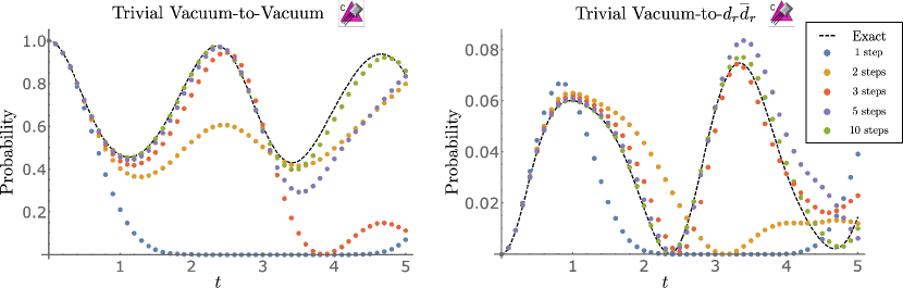
Figure 14: The trivial vacuum-to-vacuum and trivial vacuum-to-$d_{r}\overline{d}_{r}$ probabilities in QCD with $N_{f}=2$ for $m=g=L=1$. Shown are the results obtained from exact exponentiation of the Hamiltonian (dashed black curve) and from the Trotterized implementation with $1$, $2$, $3$, $5$ and $10$ Trotter steps using the (classical) quantum simulators in cirq and qiskit (denoted by the purple icons [38]).

The number of Trotter steps, $N_{\rm Trott}$, required to evolve out to a given $t$ within a specified (systematic) error, $\epsilon_{\rm Trott}$, was also investigated. $\epsilon_{\rm Trott}$ is defined as the maximum fractional error between the Trotterized and exact time evolution in two quantities, the vacuum-to-vacuum persistence probability and the vacuum-to-$d_{r}\overline{d}_{r}$ transition probability. For demonstrative purposes, an analysis at leading order in the Trotter expansion is sufficient. Naive expectations based upon global properties of the Hamiltonian defining the evolution operators indicate that an upper bound for $\epsilon_{\rm Trott}$ scales as

$$\Big{\lvert}\Big{\lvert}e^{-iHt}-\left[U_{1}\left(\frac{t}{N_{\rm Trott}}\right)\right]^{N_{\rm Trott}}\Big{\rvert}\Big{\rvert}\ \leq\ \frac{1}{2}\sum_{i}\sum_{j>i}\Big{\lvert}\Big{\lvert}\left[H_{i},H_{j}\right]\Big{\rvert}\Big{\rvert}\frac{t^{2}}{N_{\rm Trott}}\ ,$$ (24)

where the Hamiltonian has been divided into sets of mutually commuting terms, $H=\sum_{i}H_{i}$. This upper bound indicates that the required number of Trotter steps to maintain a fixed error scales as $N_{\rm Trott}\sim t^{2}$ [184].

To explore the resource requirements for simulation based upon explicit calculations between exclusive states, as opposed to upper bounds for inclusive processes, given in Eq. (24), a series of calculations was performed requiring $\epsilon_{\rm Trott}\leq 0.1$ for a range of times, $t$. Figure 15 shows the required $N_{\rm Trott}$ as a function of $t$ for $m=g=L=1$.

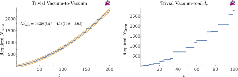
Figure 15: The number of Trotter steps, $N_{\rm Trott}$, required to achieve a systematic fractional error of $\epsilon_{{\rm Trott}}\leq 0.1$ at time $t$ in the trivial vacuum-to-vacuum probability (left panel) and the trivial vacuum-to-$d_{r}\overline{d}_{r}$ probability (right panel) for QCD with $N_{f}=2$ and $m=g=L=1$. The blue points are results obtained by direct calculation.

The plateaus observed in Fig. 15 arise from resolving upper bounds from oscillating functions, and introduce a limitation in fitting to extract scaling behavior. This is less of a limitation for the larger vacuum-to-vacuum probabilities which are fit well by a quadratic polynomial, starting from $t=1$, with coefficients,

$$N_{{\rm Trott}}=0.0393(5)t^{2}+4.13(10)t-22(5)\ .$$ (25)

The uncertainty represents a 95% confidence interval in the fit parameters and corresponds to the shaded orange region in Fig. 15. The weak quadratic scaling with $t$ implies that, even out to $t\sim 100$, the number of Trotter steps scales approximately linearly, and a constant error in the observables can be achieved with a fixed Trotter step size. We have been unable to distinguish between fits with and without logarithmic terms.

These results can be contrasted with those obtained for the Schwinger model in Weyl gauge. The authors of Ref. [129] estimate a resource requirement, as quantified by the number of $T$-gates, that scales as $\sim(Lt)^{3/2}\log Lt$, increasing to $\sim L^{5/2}t^{3/2}\log Lt\log L$ if the maximal value of the gauge fields is accommodated within the Hilbert space. The results obtained in this section suggest that resource requirements in axial gauge, as quantified by the number of CNOTs, effectively scale as $\sim L^{2}t$ up to intermediate times and as $\sim L^{2}t^{2}$ asymptotically. In a scattering process with localized wave-packets, it is appropriate to take $L\sim t$ (for the speed of light taken to be $c=1$), as the relevant non-trivial time evolution is bounded by the light cone. This suggests that the required resources scale asymptotically as $\sim t^{4}$, independent of the chosen gauge to define the simulation. This could have been anticipated at the outset by assuming that the minimum change in complexity for a process has physical meaning [185, 186, 187, 188].

III Simulating $1+1$D QCD with $N_{f}=1$ and $L=1$

With the advances in quantum devices, algorithms and mitigation strategies, quantum simulations of $1+1$D QCD can now begin, and this section presents results for $N_{f}=1$ and $L=1$. Both state preparation and time evolution will be discussed.

III.1 State Preparation with VQE

Restricting the states of the lattice to be color singlets reduces the complexity of state preparation significantly. Transformations in the quark sector are mirrored in the antiquark sector. A circuit that prepares the most general state with $r=g=b=0$ is shown in Fig. 16.

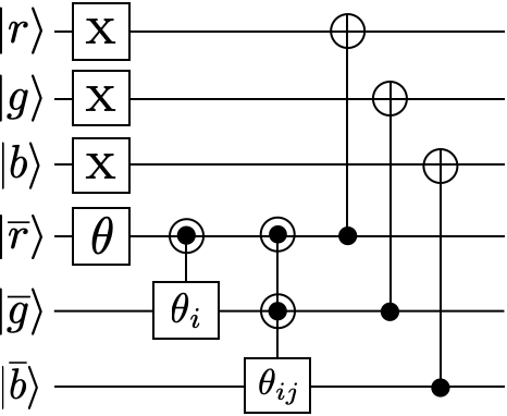
Figure 16: Building upon the trivial vacuum, this circuit initializes the most general real wavefunction (with 7 independent rotation angles for 3 qubits) in the $\overline{q}$-sector, which is subsequently mirrored into the $q$-sector by 3 CNOTs. Gates labelled by “$\theta$” are shorthand for $R_{Y}(\theta)$ and half-filled circles denote a control on $0$ and a different control on $1$.

The (multiply-)controlled $\theta$ gates are short-hand for (multiply-)controlled $R_{Y}(\theta)$ gates with half-filled circles denoting a control on $0$ and a different control on $1$. The subscripts on $\theta_{ij}$ signify that there are different angles for each controlled rotation. For example, $\theta_{i}$ has two components, $\theta_{0}$ and $\theta_{1}$, corresponding to a rotation controlled on $0$ and $1$, respectively. The CNOTs at the end of the circuit enforce that there are equal numbers of quarks and antiquarks with the same color, i.e., that $r=g=b=0$. This circuit can be further simplified by constraining the angles to only parameterize color singlet states. The color singlet subspace is spanned by

$$\ket{{\Omega_{0}}}\ ,\ \ \frac{1}{\sqrt{3}}\left(\ket{q_{r}\overline{q}_{r}}-\ket{q_{g}\overline{q}_{g}}+\ket{q_{b}\overline{q}_{b}}\right)\ ,$$

$$\ket{q_{r}\overline{q}_{r}\,q_{g}\overline{q}_{g}\,q_{b}\overline{q}_{b}}\ ,\ \ \frac{1}{\sqrt{3}}\left(\ket{q_{r}\overline{q}_{r}\,q_{g}\overline{q}_{g}}-\ket{q_{r}\overline{q}_{r}\,q_{b}\overline{q}_{b}}+\ket{q_{g}\overline{q}_{g}\,q_{b}\overline{q}_{b}}\right)\ ,$$ (26)

where $\ket{{\Omega_{0}}}=\ket{{000111}}$ is the trivial vacuum. This leads to the following relations between angles,

$$\theta_{10} =\theta_{01}\ , \theta_{00} =-2\sin^{-1}\left[\tan(\theta_{0}/2)\,\cos(\theta_{01}/2)\right]\ ,$$

$$\theta_{01} =-2\sin^{-1}\left[\cos(\theta_{11}/2)\,\tan(\theta_{1}/2)\right]\ , \theta_{0} =-2\sin^{-1}\left[\tan(\theta/2)\,\cos(\theta_{1}/2)\right]\ .$$ (27)

The circuit in Fig. 16 can utilize the strategy outlined in Ref. [105] to separate into a “variational” part and a “static” part. If the VQE circuit can be written as $U_{var}(\theta)U_{s}$, where $U_{s}$ is independent of the variational parameters, then $U_{s}$ can be absorbed by a redefinition of the Hamiltonian. Specifically, matrix elements of the Hamiltonian can be written as

$$\bra{{\Omega_{0}}}U_{var}^{\dagger}(\theta)\tilde{H}U_{var}(\theta)\ket{{\Omega_{0}}}\ ,$$ (28)

where $\tilde{H}=U_{s}^{\dagger}HU_{s}$. Table 5 shows the transformations of various Pauli strings under conjugation by a CNOT controlled on the smaller index qubit. Note that the $\mathbb{Z}_{2}$ nature of this transformation is manifest.

$XX\to IX$	$XY\to IY$	$YX\to ZY$	$XZ\to XZ$	$ZZ\to ZI$	$YZ\to YI$	$ZY\to YX$	$YY\to(-)ZX$
$IX\to XX$	$IY\to XY$	$XI\to XI$	$IZ\to IZ$	$ZI\to ZZ$	$YI\to YZ$	$ZX\to(-)YY$	$II\to II$

Table 5: The transformation of Pauli strings under conjugation by a CNOT controlled on the smaller index qubit.

In essence, entanglement is traded for a larger number of correlated measurements. Applying the techniques in Ref. [38], the VQE circuit of Fig. 16 can be put into the form of Fig. 17, which requires $5$ CNOTs along with all-to-all connectivity between the three $\overline{q}$s.

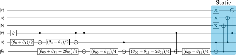
Figure 17: A circuit that initializes the most general $B=0$ color singlet state for $N_{f}=1$ and $L=1$. Gates labelled by “$\theta$” are shorthand for $R_{Y}(\theta)$ and the $X$s at the end are to initialize the trivial vacuum. The color singlet constraint, $\theta_{10}=\theta_{01}$, has been used and the other angles are related by Eq. (27).

III.2 Time Evolution Using IBM’s 7-Qubit Quantum Computers

A single leading-order Trotter step of $N_{f}=1$ QCD with $L=1$ requires 28 CNOTs. A circuit that implements one Trotter step of the mass term is shown in Fig. 18.

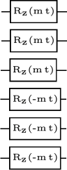
Figure 18: A circuit that implements $U_{m}(t)=\exp(-iH_{m}t)$ for $N_{f}=1$ and $L=1$.

As discussed around Eq. (20), it is more efficient to not use an ancilla qubit in the Trotterization of the kinetic part of the Hamiltonian. A circuit that implements one Trotter step of a single hopping term is shown in Fig. 19 [172].

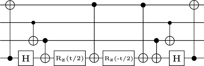
Figure 19: A circuit that implements $\exp[-i\frac{t}{2}(\sigma^{+}ZZ\sigma^{-}+{\rm h.c.})]$.

Similarly, for this system, the only contribution to $H_{el}$ is $Q^{(a)}_{n}\,Q^{(a)}_{n}$, which contains three $ZZ$ terms that are Trotterized using the standard two CNOT implementation. The complete set of circuits required for Trotterized time evolution are given in App. E.

To map the system onto a quantum device, it is necessary to understand the required connectivity for efficient simulation. Together, the hopping and chromo-electric terms require connectivity between nearest neighbors as well as between $q_{r}$ and $q_{b}$ and $q$s and $\overline{q}$s of the same color. The required device topology is planar and two embedding options are shown in Fig. 20.

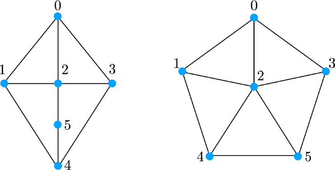
Figure 20: Two potential quantum device topologies for the implementation of Trotterized time evolution.

The “kite” topology follows from the above circuits, while the “wagon wheel” topology makes use of the identities $CX(q_{a},q_{b})\cdot CX(q_{b},q_{c})=CX(q_{a},q_{c})\cdot CX(q_{b},q_{c})=CX(q_{b},q_{a})\cdot CX(q_{a},q_{c})$ where $CX(q_{a},q_{b})$ denotes a CNOT controlled on qubit $q_{a}$. Both topologies can be employed on devices with all-to-all connectivity, such as trapped-ion systems, but neither topology exists natively on available superconducting-qubit devices.

We performed leading-order Trotter evolution to study the trivial vacuum persistence and transition probability using IBM’s quantum computers ibmq_jakarta and ibm_perth, each a r5.11H quantum processor with 7 qubits and “H”-connectivity. The circuits developed for this system require a higher degree of connectivity than available with these devices, and so SWAP-gates were necessary for implementation. The IBM transpiler was used to first compile the circuit for the H-connectivity and then again to compile the Pauli twirling (discussed next). An efficient use of SWAP-gates allows for a single Trotter step to be executed with 34 CNOTs.

A number of error-mitigation techniques were employed to minimize associated systematic uncertainties in our calculations: randomized compiling of the CNOTs (Pauli twirling) [189] combined with decoherence renormalization [190, 71], measurement error mitigation, post-selecting on physical states and dynamical decoupling [191, 192, 193, 194]. The circuits were randomly complied with each CNOT Pauli-twirled as a mechanism to transform coherent errors in the CNOT gates into statistical noise in the ensemble. This has been shown to be effective in improving the quality of results in other simulations, for example, Refs. [174, 71]. Pauli twirling involves multiplying the right side of each CNOT by a randomly chosen element of the two-qubit Pauli group, $G_{2}$, and the left side by $G^{\prime}_{2}$ such that $G^{\prime}_{2}\,CX\,G_{2}=CX$ (up to a phase). For an ideal CNOT gate, this would have no effect on the circuit. A table of required CNOT identities is given, for example, in an appendix in Ref. [71]. Randomized Pauli-twirling is combined with performing measurements of a “non-physics”, mitigation circuit, which is the time evolution circuit evaluated at $t=0$, and is the identity in the absence of noise. Assuming that the randomized-compiling of the Pauli-twirled CNOTs transforms coherent noise into depolarizing noise, the fractional deviation of the noiseless and computed results from the asymptotic limit of complete decoherence are expected to be approximately equal for both the physics and mitigation ensembles. Assuming linearity, it follows that

$$\left(P_{\text{pred}}^{(\text{phys})}-\frac{1}{8}\right)=\left(P_{\text{meas}}^{(\text{phys})}-\frac{1}{8}\right)\times\left(\frac{1-\frac{1}{8}}{P_{\text{meas}}^{(\text{mit})}-\frac{1}{8}}\right)\ ,$$ (29)

where $P_{\text{meas}}^{(\text{phys})}$ and $P_{\text{meas}}^{(\text{mit})}$ are post-processed probabilities and $P_{\text{pred}}^{(\text{phys})}$ is an estimate of the probability once the effects of depolarizing noise have been removed. The “$\frac{1}{8}$” represents the fully decohered probability after post-selecting on physical states (described next) and the “$1$” is the probability of measuring the initial state from the mitigation circuit in the absence of noise.

The computational basis of 6 qubits contains $2^{6}$ states but time evolution only connects those with the same $r$, $g$ and $b$. Starting from the trivial vacuum, this implies that only the $8$ states with $r=g=b=0$ are accessible through time evolution. The results off the quantum computer were post-processed to only select events that populated 1 of the 8 physically allowed states, discarding outcomes that were unphysical. Typically, this resulted in a retention rate of $\sim 30\%$. The workflow interspersed physics and mitigation circuits to provide a correlated calibration of the quantum devices. This enabled the detection (and removal) of out-of-specs device performance during post-processing. We explored using the same twirling sequences for both physics and mitigation circuits and found that it had no significant impact. The impact of dynamical decoupling of idle qubits using qiskit’s built in functionality was also investigated and found to have little effect. The results of each run were corrected for measurement error using IBM’s available function, TensoredMeasFitter, and associated downstream operations.

The results obtained for the trivial vacuum-to-vacuum and trivial vacuum-to-$q_{r}\overline{q}_{r}$ probabilities from one step of leading-order Trotter time evolution are shown in Fig. 21. For each time, 447 Pauli-twirled physics circuits and 447 differently twirled circuits with zeroed angles (mitigation) were analyzed using $10^{3}$ shots on both ibmq_jakarta and ibm_perth (to estimate device systematics). After post-selecting on physical states, correlated Bootstrap Resampling was used to form the final result.

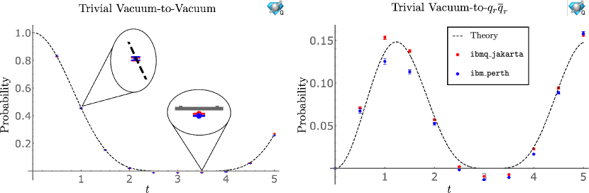
Figure 21: The trivial vacuum-to-vacuum (left panel) and trivial vacuum-to-$q_{r}\overline{q}_{r}$ (right panel) probabilities for $N_{f}=1$ QCD and $m=g=L=1$. The dashed-black curve shows the expected result from one step of leading-order Trotter evolution. The results, given in Tables 6 and 7, were obtained by using $10^{3}$ shots for 447 Pauli-twirled circuits using IBM’s quantum computers ibmq_jakarta (red) and ibm_perth (blue).

Tables 6 and 7 display the results of the calculations performed using ibmq_jakarta and ibm_perth quantum computers. The same mitigation data was used for both the trivial vacuum-to-vacuum and trivial vacuum-to-$q_{r}\overline{q}_{r}$ calculations, and is provided in columns 2 and 4 of Table 6. See App. G for an extended discussion of leading-order Trotter. Note that the negative probabilities seen in Fig. 21 indicate that additional non-linear terms are needed in Eq. (29).

Vacuum-to-Vacuum Probabilities for $N_{f}=1$ QCD from IBM’s ibmq_jakarta and ibm_perth
$t$	Mitigation jakarta	Physics jakarta	Mitigation perth	Physics perth	Results jakarta	Results perth	Theory
0	-	-	-	-	-	-	1
0.5	0.9176(10)	0.7607(24)	0.8744(23)	0.7310(42)	0.8268(27)	0.8326(52)	0.8274
1.0	0.9059(12)	0.4171(32)	0.9118(16)	0.4211(39)	0.4523(36)	0.4543(43)	0.4568
1.5	0.9180(12)	0.1483(16)	0.9077(17)	0.1489(23)	0.1507(17)	0.1518(25)	0.1534
2.0	0.8953(15)	0.0292(08)	0.8953(21)	0.0324(10)	0.0162(09)	0.0198(11)	0.0249
2.5	0.9169(12)	0.0020(01)	0.8938(21)	0.0032(02)	-0.0109(03)	-0.0136(04)	0.0010
3.0	0.9282(13)	0.00010(2)	0.9100(13)	0.00017(3)	-0.0111(02)	-0.0140(02)	$1.3\times 10^{-7}$
3.5	0.9357(10)	0.00017(3)	0.9109(14)	0.00037(4)	-0.0097(02)	-0.0138(02)	$3.2\times 10^{-5}$
4.0	0.9267(13)	0.0081(03)	0.9023(14)	0.0076(03)	-0.0026(04)	-0.0072(04)	0.0052
4.5	0.9213(12)	0.0653(10)	0.8995(16)	0.0619(11)	0.0594(11)	0.0537(13)	0.0614
5.0	0.9105(12)	0.2550(26)	0.9031(14)	0.2405(21)	0.2698(29)	0.2550(23)	0.2644

Table 6: The trivial vacuum-to-vacuum probabilities for $m=g=L=1$ using ibmq_jakarta and ibm_perth, the underlying distributions of which are displayed in Fig. 22. The 2nd through 5th columns are the results after selecting only physical states and columns $6$ and $7$ are the results after using the mitigation circuit to account for depolarizing noise.

Vacuum-to-$q_{r}\overline{q}_{r}$ Probabilities for $N_{f}=1$ QCD from IBM’s ibmq_jakarta and ibm_perth
$t$	Physics jakarta	Physics perth	Results jakarta	Results perth	Theory
0	-	-	-	-	0
0.5	0.0760(12)	0.0756(22)	0.0709(13)	0.0673(26)	0.0539
1.0	0.1504(19)	0.1253(32)	0.1534(22)	0.1254(36)	0.1363
1.5	0.1364(15)	0.1144(21)	0.1376(17)	0.1131(23)	0.1332
2.0	0.0652(11)	0.0611(15)	0.0571(13)	0.0525(17)	0.0603
2.5	0.0136(04)	0.0137(06)	0.0019(05)	-0.0017(07)	0.0089
3.0	0.0017(01)	0.0011(01)	-0.0093(02)	-0.0132(02)	$2.5\times 10^{-5}$
3.5	0.0024(01)	0.0032(02)	-0.0073(02)	-0.0107(03)	0.0010
4.0	0.0314(07)	0.0288(07)	0.0228(08)	0.0167(08)	0.0248
4.5	0.0971(12)	0.0929(14)	0.0943(13)	0.0887(16)	0.0943
5.0	0.1534(20)	0.1546(19)	0.1566(22)	0.1583(21)	0.1475

Table 7: The trivial vacuum-to-$q_{r}\overline{q}_{r}$ probabilities for $m=g=L=1$ using ibmq_jakarta and ibm_perth. The 2nd and 3rd columns are the results after selecting only physical states and columns 4 and 5 are the results after using the mitigation circuit to account for depolarizing noise.

It is interesting to consider the distributions of events obtained from the Pauli-twirled circuits, as shown in Fig. 22.

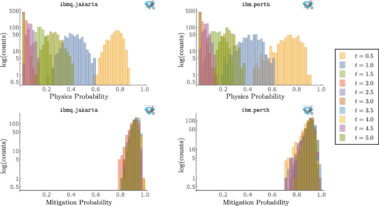
Figure 22: Histograms of the post-processed vacuum-to-vacuum results obtained using ibmq_jakarta and ibm_perth. The horizontal axes show the value of the vacuum-to-vacuum probability, and the vertical axes show bin counts on a log-scale. The top panels display the results obtained from the physics circuits for the range of evolution times and the bottom panels display the results obtained for the corresponding mitigation circuits.

The distributions are not Gaussian and, in a number of instances, exhibit heavy tails particularly near the boundaries. The spread of the distributions, associated with non-ideal CNOT gates, is seen to reach a maximum of $\sim 0.4$, but with a full-width at half-max that is $\sim 0.2$. These distributions are already broad with a 34 CNOT circuit, and we probed the limit of these devices by time-evolving with two first-order Trotter steps, which requires 91 CNOTs after accounting for SWAPs. Using the aforementioned techniques, this was found to be beyond the capabilities of ibmq_jakarta, ibmq_lagos and ibm_perth.

IV Arbitrary $N_{c}$ and $N_{f}$

In this section, the structure of the Hamiltonian for $N_{f}$ flavors of quarks in the fundamental representation of $SU(N_{c})$ is developed. The mapping to spins has the same structure as for $N_{f}=2$ QCD, but now, there are $N_{c}\times N_{f}$ $q$s and $N_{c}\times N_{f}$ $\overline{q}$s per spatial lattice site. While the mass and kinetic terms generalize straightforwardly, the energy in the chromo-electric field is more tricky. After enforcing Gauss’s law, it is

$$H_{el}=\frac{g^{2}}{2}\sum_{n=0}^{2L-2}\left(\sum_{m\leq n}Q^{(a)}_{m}\right)^{2}\ ,\ \ Q^{(a)}_{m}=\phi^{\dagger}_{m}T^{a}\phi_{m}\ ,$$ (30)

where $T^{a}$ are now the generators of $SU(N_{c})$. The Hamiltonian, including chemical potentials for baryon number (chemical potentials for other flavor combinations can be included as needed), is found to be

$$H= \ H_{kin}\ +\ H_{m}\ +\ H_{el}\ +\ H_{\mu_{B}}\ ,$$ (31a)

$$H_{kin}= \ \frac{1}{2}\sum_{n=0}^{2L-2}\sum_{f=0}^{N_{f}-1}\sum_{c=0}^{N_{c}-1}\left[\sigma_{i(n,f,c)}^{+}\left(\bigotimes_{j=1}^{N_{c}N_{f}-1}(-\sigma_{i(n,f,c)+j}^{z})\right)\sigma_{i(n,f,c)+N_{c}N_{f}}^{-}+\rm{h.c.}\right]\ ,$$ (31b)

$$H_{m}= \ \frac{1}{2}\sum_{n=0}^{2L-1}\sum_{f=0}^{N_{f}-1}\sum_{c=0}^{N_{c}-1}m_{f}\left[(-1)^{n}\sigma^{z}_{i(n,f,c)}+1\right]\ ,$$ (31c)

$$H_{el}= \ \frac{g^{2}}{2}\sum_{n=0}^{2L-2}(2L-1-n)\left(\sum_{f=0}^{N_{f}-1}Q_{n,f}^{(a)}\,Q_{n,f}^{(a)}\ \ +\ \ 2\sum_{f=0}^{N_{f}-2}\sum_{f^{\prime}=f+1}^{N_{f}-1}Q_{n,f}^{(a)}\,Q_{n,f^{\prime}}^{(a)}\right)$$

$$+g^{2}\sum_{n=0}^{2L-3}\sum_{m=n+1}^{2L-2}(2L-1-m)\sum_{f=0}^{N_{f}-1}\sum_{f^{\prime}=0}^{N_{f}-1}Q_{n,f}^{(a)}\,Q_{m,f^{\prime}}^{(a)}\ ,$$ (31d)

$$H_{\mu_{B}}= \ -\frac{\mu_{B}}{2N_{c}}\sum_{n=0}^{2L-1}\sum_{f=0}^{N_{f}-1}\sum_{c=0}^{N_{c}-1}\sigma^{z}_{i(n,f,c)}\ ,$$ (31e)

where, $i(n,f,c)=(N_{c}N_{f}n+N_{f}f+c)$, and the products of the charges are

$$4Q_{n,f}^{(a)}\,Q_{n,f}^{(a)}= \ \frac{N_{c}^{2}-1}{2}-\left(1+\frac{1}{N_{c}}\right)\sum_{c=0}^{N_{c}-2}\sum_{c^{\prime}=c+1}^{N_{c}-1}\sigma^{z}_{i(n,f,c)}\sigma^{z}_{i(n,f,c^{\prime})}\ ,$$

$$8Q_{n,f}^{(a)}\,Q_{m,f^{\prime}}^{(a)}= \ 4\sum_{c=0}^{N_{c}-2}\sum_{c^{\prime}=c+1}^{N_{c}-1}\left[\sigma^{+}_{i(n,f,c)}\ \left(\otimes Z\right)_{(n,f,c,c^{\prime})}\ \sigma^{-}_{i(n,f,c^{\prime})}\sigma^{-}_{i(m,f^{\prime},c)}\ \left(\otimes Z\right)_{(m,f^{\prime},c,c^{\prime})}\ \sigma^{+}_{i(m,f^{\prime},c^{\prime})}+{\rm h.c.}\right]\$$

$$+\sum_{c=0}^{N_{c}-1}\sum_{c^{\prime}=0}^{N_{c}-1}\left(\delta_{cc^{\prime}}-\frac{1}{N_{c}}\right)\sigma^{z}_{i(n,f,c)}\sigma^{z}_{i(m,f^{\prime},c^{\prime})}\ ,$$

$$\left(\otimes Z\right)_{(n,f,c,c^{\prime})}\equiv \ \bigotimes_{k=1}^{c^{\prime}-c-1}\sigma^{z}_{i(n,f,c)+k}\ .$$ (32)

The resource requirements for implementing Trotterized time evolution using generalizations of the circuits in Sec. II.3 are given in Eq. (21).

It is interesting to consider the large-$N_{c}$ limit of the Hamiltonian, where quark loops are parametrically suppressed and the system can be described semi-classically [106, 107, 198, 199]. Unitarity requires rescaling the strong coupling, $g^{2}\to g^{2}/N_{c}$ and leading terms in the Hamiltonian scale as $\mathcal{O}(N_{c})$. The leading order contribution to the product of charges is

$$4Q_{n,f}^{(a)}\,Q_{n,f}^{(a)}= \ \sum_{c=0}^{N_{c}-2}\sum_{c^{\prime}=c+1}^{N_{c}-1}\left(1-\sigma^{z}_{i(n,f,c)}\sigma^{z}_{i(n,f,c^{\prime})}\right)\ ,$$

$$8Q_{n,f}^{(a)}\,Q_{m,f^{\prime}}^{(a)}= \ 4\sum_{c=0}^{N_{c}-2}\sum_{c^{\prime}=c+1}^{N_{c}-1}\left[\sigma^{+}_{i(n,f,c)}\ \left(\otimes Z\right)_{(n,f,c,c^{\prime})}\ \sigma^{-}_{i(n,f,c^{\prime})}\sigma^{-}_{i(m,f^{\prime},c)}\ \left(\otimes Z\right)_{(m,f^{\prime},c,c^{\prime})}\ \sigma^{+}_{i(m,f^{\prime},c^{\prime})}+{\rm h.c.}\right]\ .$$ (33)

Assuming that the number of $q\overline{q}$ pairs that contribute to the meson wavefunctions do not scale with $N_{c}$, as expected in the large-$N_{c}$ limit, $H_{el}\propto N_{c}$ and mesons are non-interacting, a well known consequence of the large-$N_{c}$ limit [106, 107]. Baryons on the other hand are expected to have strong interactions at leading order in $N_{c}$ [198]. This is a semi-classical limit and we expect that there exists a basis where states factorize into localized tensor products, and the time evolution operator is non-entangling. The latter result has been observed in the large-$N_{c}$ limit of hadronic scattering [153, 154, 155, 200, 201].

V Summary and Discussion

Important for future quantum simulations of processes that can be meaningfully compared to experiment, the real-time dynamics of strongly-interacting systems are predicted to be efficiently computable with quantum computers of sufficient capability. Building upon foundational work in quantum chemistry and in low-dimensional $U(1)$ and $SU(2)$ gauge theories, this work has developed the tools necessary for the quantum simulation of $1+1$D QCD (in axial gauge) using open boundary conditions, with arbitrary numbers of quark flavors and colors and including chemical potentials for baryon number and isospin. Focusing largely on QCD with $N_{f}=2$, which shares many of the complexities of QCD in $3+1$D, we have performed a detailed analysis of the required quantum resources for simulation of real-time dynamics, including efficient quantum circuits and associated gate counts, and the scaling of the number of Trotter steps for a fixed-precision time evolution. The structure and dynamics of small systems, with $L=1,2$ for $N_{c}=3$ and $N_{f}=1,2$ have been detailed using classical computation, quantum simulators, D-Wave’s Advantage and IBM’s 7-qubit devices ibmq_jakarta and ibm_perth. Using recently developed error mitigation strategies, relatively small uncertainties were obtained for a single Trotter step with $34$ CNOT gates after transpilation onto the QPU connectivity.

Through a detailed study of the low-lying spectrum, both the relevant symmetries and the color-singlets in the mesonic and baryonic sectors, including a bound two-baryon nucleus, have been identified. Open boundary conditions also permit low-lying color edge-states that penetrate into the lattice volume by a distance set by the confinement scale. By examining quark entanglement in the hadrons, a transition from the mesons being primarily composed of quark-antiquarks to baryon-antibaryons was found. We have presented the relative contributions of each of the terms in the Hamiltonian to the energy of the vacuum, mesons and baryons.

This work has provided an estimate for the number of CNOT-gates required to implement one Trotter step in $N_{f}=2$, $1+1$D axial-gauge QCD. For $L=10$ spatial sites, $\sim 3\times 10^{4}$ CNOTs are required, while $\sim 4\times 10^{6}$ CNOTs are required for $L=100$. Realistically, quantum simulations with $L=10$ are a beginning toward providing results with a complete quantification of uncertainties, including lattice-spacing and finite-volume artifacts, and $L=100$ will likely yield high-precision results. It was found that, in the axial-gauge formulation, resources for time evolution effectively scale as $L^{2}t$ for intermediate times and $L^{2}t^{2}$ for asymptotic times. With $L\sim t$, this asymptotic scaling is the same as in the Schwinger model, suggesting no differences in scaling between Weyl and axial gauges.

Appendix A Mapping to Qubits

This appendix outlines how the qubit Hamiltonian in Eq. (6) is obtained from the lattice Hamiltonian in Eq. (3). For this system, the constraint of Gauss’s law is sufficient to uniquely determine the chromo-electric field carried by the links between lattice sites in terms of a background chromo-electric field and the distribution of color charges. The difference between adjacent chromo-electric fields at a site with charge $Q^{(a)}$ is

$${\bf E}^{(a)}_{n+1}-{\bf E}^{(a)}_{n}=Q^{(a)}_{n}\ ,$$ (34)

for $a=1$ to $8$, resulting in a chromo-electric field

$${\bf E}^{(a)}_{n}={\bf F}^{(a)}\>+\>\sum_{i\leq n}Q^{(a)}_{i}\ .$$ (35)

In general, there can be a non-zero background chromo-electric field, ${\bf F}^{(a)}$, which in this paper has been set to zero. Inserting the chromo-electric field in terms of the charges into Eq. (1) yields Eq. (3).

The color and flavor degrees of freedom of each $q$ and $\overline{q}$ are then distributed over $6$ ($=N_{c}N_{f}$) sites as illustrated in Fig. (1). There are now creation and annihilation operators for each quark, and the Hamiltonian is

$$H= \ \sum_{n=0}^{2L-1}\sum_{f=0}^{1}\sum_{c=0}^{2}\left[m_{f}(-1)^{n}\psi^{\dagger}_{6n+3f+c}\psi_{6n+3f+c}\>-\>\frac{\mu_{B}}{3}\psi^{\dagger}_{6n+3f+c}\psi_{6n+3f+c}\>-\>\frac{\mu_{I}}{2}(-1)^{f}\psi^{\dagger}_{6n+3f+c}\psi_{6n+3f+c}\right]$$

$$+\frac{1}{2}\sum_{n=0}^{2L-2}\sum_{f=0}^{1}\sum_{c=0}^{2}\left(\psi^{\dagger}_{6n+3f+c}\psi_{6(n+1)+3f+c}+\>{\rm h.c.}\right)\>+\>\frac{g^{2}}{2}\sum_{n=0}^{2L-2}\left(\sum_{m\leq n}\sum_{f=0}^{1}Q^{(a)}_{m,f}\right)^{2}\ ,$$ (36)

where the color charge is evaluated over three $(r,g,b)$ occupation sites with the same flavor,

$$Q_{m,f}^{(a)}=\sum_{c=0}^{2}\sum_{c^{\prime}=0}^{2}\psi^{\dagger}_{6m+3f+c}\ T^{a}_{cc^{\prime}}\ \psi_{6m+3f+c^{\prime}}\ ,$$ (37)

and the $T^{a}$ are the eight generators of $SU(3)$. The fermionic operators in Fock space are mapped onto spin operators via the JW transformation,

$$\psi_{n}=\bigotimes_{l<n}(-\sigma^{z}_{l})\sigma^{-}_{n}\ ,\ \ \psi_{n}^{\dagger}=\bigotimes_{l<n}(-\sigma^{z}_{l})\sigma^{+}_{n}\ .$$ (38)

In terms of spins, the eight $SU(3)$ charge operators become

$$Q_{m,f}^{(1)}= \ \frac{1}{2}\sigma^{+}_{6m+3f}\sigma^{-}_{6m+3f+1}+\rm{h.c.}\ ,$$

$$Q_{m,f}^{(2)}= \ -\frac{i}{2}\sigma^{+}_{6m+3f}\sigma^{-}_{6m+3f+1}+\rm{h.c.}\ ,$$

$$Q_{m,f}^{(3)}= \ \frac{1}{4}(\sigma^{z}_{6m+3f}-\sigma^{z}_{6m+3f+1})\ ,$$

$$Q_{m,f}^{(4)}= \ -\frac{1}{2}\sigma^{+}_{6m+3f}\sigma^{z}_{6m+3f+1}\sigma^{-}_{6m+3f+2}+\rm{h.c.}\ ,$$

$$Q_{m,f}^{(5)}= \ \frac{i}{2}\sigma^{+}_{6m+3f}\sigma^{z}_{6m+3f+1}\sigma^{-}_{6m+3f+2}+\rm{h.c.}\ ,$$

$$Q_{m,f}^{(6)}= \ \frac{1}{2}\sigma^{+}_{6m+3f+1}\sigma^{-}_{6m+3f+2}+\rm{h.c.}\ ,$$

$$Q_{m,f}^{(7)}= \ -\frac{i}{2}\sigma^{+}_{6m+3f+1}\sigma^{-}_{6m+3f+2}+\rm{h.c.}\ ,$$

$$Q_{m,f}^{(8)}= \ \frac{1}{4\sqrt{3}}(\sigma^{z}_{6m+3f}+\sigma^{z}_{6m+3f+1}-2\sigma^{z}_{6m+3f+2})\ .$$ (40)

Substituting Eqs. (38) and (40) into Eq. (36) gives the Hamiltonian in Eq. (6). For reference, the expanded Hamiltonian for $L=1$ is

$$H= \ H_{kin}\ +\ H_{m}\ +\ H_{el}\ +\ H_{\mu_{B}}\ +\ H_{\mu_{I}}\ ,$$ (41a)

$$H_{kin}= \ -\frac{1}{2}(\sigma^{+}_{6}\sigma^{z}_{5}\sigma^{z}_{4}\sigma^{z}_{3}\sigma^{z}_{2}\sigma^{z}_{1}\sigma^{-}_{0}+\sigma^{-}_{6}\sigma^{z}_{5}\sigma^{z}_{4}\sigma^{z}_{3}\sigma^{z}_{2}\sigma^{z}_{1}\sigma^{+}_{0}+\sigma^{+}_{7}\sigma^{z}_{6}\sigma^{z}_{5}\sigma^{z}_{4}\sigma^{z}_{3}\sigma^{z}_{2}\sigma^{-}_{1}+\sigma^{-}_{7}\sigma^{z}_{6}\sigma^{z}_{5}\sigma^{z}_{4}\sigma^{z}_{3}\sigma^{z}_{2}\sigma^{+}_{1}$$

$$+\,\sigma^{+}_{8}\sigma^{z}_{7}\sigma^{z}_{6}\sigma^{z}_{5}\sigma^{z}_{4}\sigma^{z}_{3}\sigma^{-}_{2}+\sigma^{-}_{8}\sigma^{z}_{7}\sigma^{z}_{6}\sigma^{z}_{5}\sigma^{z}_{4}\sigma^{z}_{3}\sigma^{+}_{2}+\sigma^{+}_{9}\sigma^{z}_{8}\sigma^{z}_{7}\sigma^{z}_{6}\sigma^{z}_{5}\sigma^{z}_{4}\sigma^{-}_{3}+\sigma^{-}_{9}\sigma^{z}_{8}\sigma^{z}_{7}\sigma^{z}_{6}\sigma^{z}_{5}\sigma^{z}_{4}\sigma^{+}_{3}$$

$$+\,\sigma^{+}_{10}\sigma^{z}_{9}\sigma^{z}_{8}\sigma^{z}_{7}\sigma^{z}_{6}\sigma^{z}_{5}\sigma^{-}_{4}+\sigma^{-}_{10}\sigma^{z}_{9}\sigma^{z}_{8}\sigma^{z}_{7}\sigma^{z}_{6}\sigma^{z}_{5}\sigma^{+}_{4}+\sigma^{+}_{11}\sigma^{z}_{10}\sigma^{z}_{9}\sigma^{z}_{8}\sigma^{z}_{7}\sigma^{z}_{6}\sigma^{-}_{5}+\sigma^{-}_{11}\sigma^{z}_{10}\sigma^{z}_{9}\sigma^{z}_{8}\sigma^{z}_{7}\sigma^{z}_{6}\sigma^{+}_{5})\ ,$$ (41b)

$$H_{m}= \ \frac{1}{2}\left[m_{u}\left(\sigma^{z}_{0}+\sigma^{z}_{1}+\sigma^{z}_{2}-\sigma^{z}_{6}-\sigma^{z}_{7}-\sigma^{z}_{8}+6\right)+m_{d}\left(\sigma^{z}_{3}+\sigma^{z}_{4}+\sigma^{z}_{5}-\sigma^{z}_{9}-\sigma^{z}_{10}-\sigma^{z}_{11}+6\right)\right]\ ,$$ (41c)

$$H_{el}= \ \frac{g^{2}}{2}\bigg{[}\frac{1}{3}(3-\sigma^{z}_{1}\sigma^{z}_{0}-\sigma^{z}_{2}\sigma^{z}_{0}-\sigma^{z}_{2}\sigma^{z}_{1})+\sigma^{+}_{4}\sigma^{-}_{3}\sigma^{-}_{1}\sigma^{+}_{0}+\sigma^{-}_{4}\sigma^{+}_{3}\sigma^{+}_{1}\sigma^{-}_{0}+\sigma^{+}_{5}\sigma^{z}_{4}\sigma^{-}_{3}\sigma^{-}_{2}\sigma^{z}_{1}\sigma^{+}_{0}+\sigma^{-}_{5}\sigma^{z}_{4}\sigma^{+}_{3}\sigma^{+}_{2}\sigma^{z}_{1}\sigma^{-}_{0}$$

$$+\,\sigma^{+}_{5}\sigma^{-}_{4}\sigma^{-}_{2}\sigma^{+}_{1}+\sigma^{-}_{5}\sigma^{+}_{4}\sigma^{+}_{2}\sigma^{-}_{1}$$

$$+\,\frac{1}{12}\left(2\sigma^{z}_{3}\sigma^{z}_{0}+2\sigma^{z}_{4}\sigma^{z}_{1}+2\sigma^{z}_{5}\sigma^{z}_{2}-\sigma^{z}_{5}\sigma^{z}_{0}-\sigma^{z}_{5}\sigma^{z}_{1}-\sigma^{z}_{4}\sigma^{z}_{2}-\sigma^{z}_{4}\sigma^{z}_{0}-\sigma^{z}_{3}\sigma^{z}_{1}-\sigma^{z}_{3}\sigma^{z}_{2}\right)\bigg{]}\ ,$$ (41d)

$$H_{\mu_{B}}= \ -\frac{\mu_{B}}{6}\left(\sigma^{z}_{0}+\sigma^{z}_{1}+\sigma^{z}_{2}+\sigma^{z}_{3}+\sigma^{z}_{4}+\sigma^{z}_{5}-\sigma^{z}_{6}+\sigma^{z}_{7}+\sigma^{z}_{8}+\sigma^{z}_{9}+\sigma^{z}_{10}+\sigma^{z}_{11}\right)\ ,$$ (41e)

$$H_{\mu_{I}}= \ -\frac{\mu_{I}}{4}\left(\sigma^{z}_{0}+\sigma^{z}_{1}+\sigma^{z}_{2}-\sigma^{z}_{3}-\sigma^{z}_{4}-\sigma^{z}_{5}+\sigma^{z}_{6}+\sigma^{z}_{7}+\sigma^{z}_{8}-\sigma^{z}_{9}-\sigma^{z}_{10}-\sigma^{z}_{11}\right)\ .$$ (41f)

Appendix B Symmetries of the Free-Quark Hamiltonian

Here the symmetries of the free-quark Hamiltonian are identified to better understand the degeneracies observed in the spectrum of $1+1$D QCD with $N_{f}=2$ and $L=1$ as displayed in Figs. 2 and 3. Specifically, the Hamiltonian with $g=h=\mu_{B}=\mu_{I}=0$, leaving only the hopping and mass terms ($m=m_{u}=m_{d}$), is

$$H=\sum_{f=0}^{1}\sum_{c=0}^{2}\left[m\sum_{n=0}^{2L-1}(-1)^{n}\psi^{\dagger}_{6n+3f+c}\psi_{6n+3f+c}\>+\>\frac{1}{2}\sum_{n=0}^{2L-2}\left(\psi^{\dagger}_{6n+3f+c}\psi_{6(n+1)+3f+c}+\>{\rm h.c.}\right)\right]\ .$$ (42)

The mapping of degrees of freedom is taken to be as shown in Fig. 1, but it will be convenient to work with Fock-space quark operators instead of spin operators. In what follows the focus will be on $L=1$, and larger systems follow similarly.

The creation operators can be assembled into a 12-component vector, $\Psi^{\dagger}_{i}=(\psi_{0}^{\dagger},\,\psi_{1}^{\dagger},\ldots,\psi_{10}^{\dagger},\,\psi_{11}^{\dagger})$, in terms of which the Hamiltonian becomes

$$H=\Psi^{\dagger}_{i}M_{ij}\Psi_{j}\ ,$$ (43)

where $M$ is a $12\times 12$ block matrix of the form,

$$M=\left[\begin{array}[]{c|c}m&1/2\\ \hline\cr 1/2&-m\end{array}\right]\ ,$$ (44)

with each block a $6\times 6$ diagonal matrix. Diagonalizing $M$, gives rise to

$$\tilde{M}=\left[\begin{array}[]{c|c}\lambda&0\\ \hline\cr 0&-\lambda\end{array}\right]\ ,\ \ \lambda=\frac{1}{2}\sqrt{1+4m^{2}}\ ,$$ (45)

with associated eigenvectors,

$$\tilde{\psi}_{i}=\frac{1}{\sqrt{2}}\left(\sqrt{1+\frac{\lambda}{m}}\,\psi_{i}\ +\ \sqrt{1-\frac{\lambda}{m}}\,\psi_{6+i}\right)\ ,\ \tilde{\psi}_{6+i}=\frac{1}{\sqrt{2}}\left(-\sqrt{1-\frac{\lambda}{m}}\,\psi_{i}\ +\ \sqrt{1+\frac{\lambda}{m}}\,\psi_{6+i}\right)\ ,$$ (46)

where $\tilde{\psi}_{i}$ ($\tilde{\psi}_{6+i}$) corresponds to the positive (negative) eigenvalue and the index $i$ takes values $0$ to $5$. These eigenvectors create superpositions of quarks and antiquarks with the same color and flavor, which are the OBC analogs of momentum plane-waves. In this basis, the Hamiltonian becomes

$$H=\sum_{i=0}^{5}\lambda\left(\tilde{\psi}^{\dagger}_{i}\tilde{\psi}_{i}-\tilde{\psi}^{\dagger}_{6+i}\tilde{\psi}_{6+i}\right)\ ,$$ (47)

which has a vacuum state,

$$\lvert\Omega_{0}\rangle=\prod_{i=0}^{i=5}\tilde{\psi}^{\dagger}_{6+i}\ket{\omega_{0}}\ ,$$ (48)

where $\ket{\omega_{0}}$ is the unoccupied state, and $\lvert\Omega_{0}\rangle$ corresponds to $\lvert 000000111111\rangle$ (in binary) in this transformed basis. Excited states are formed by acting with either $\tilde{\psi}^{\dagger}_{i}$ or $\tilde{\psi}_{6+i}$ on $\lvert\Omega_{0}\rangle$ which raises the energy of the system by $\lambda$. A further transformation is required for the $SU(12)$ symmetry to be manifest. In terms of the 12-component vector, $\tilde{\Psi}^{\dagger}=(\tilde{\psi}^{\dagger}_{0},\,\ldots,\,\tilde{\psi}^{\dagger}_{5},\,\tilde{\psi}_{6},\,\ldots,\,\tilde{\psi}_{11})$, the Hamiltonian in Eq. (47) becomes,

$$H=\sum_{i=0}^{5}\lambda\left(\tilde{\psi}^{\dagger}_{i}\tilde{\psi}_{i}-\tilde{\psi}^{\dagger}_{6+i}\tilde{\psi}_{6+i}\right)\ =\ \lambda\left(\tilde{\Psi}^{\dagger}\tilde{\Psi}-6\right)\ ,$$ (49)

where the canonical anticommutation relations have been used to obtain the final equality. This is invariant under a $SU(12)$ symmetry, where $\tilde{\Psi}$ transforms in the fundamental representation. The free-quark spectrum ($g=h=0$) is therefore described by states with degeneracies corresponding to the ${\bf 1}$ and ${\bf 12}$ of $SU(12)$ as well as the antisymmetric combinations of fundamental irreps, ${\bf 66},{\bf 220},\ldots$ as illustrated in Figs. 2 and 3. The vacuum state corresponds to the singlet of $SU(12)$. The lowest-lying 12 corresponds to single quark or antiquark excitations, which are color ${\bf 3}_{c}$s for quarks and $\overline{\bf 3}_{c}$s for antiquarks and will each appear as isodoublets, i.e., ${\bf 12}\rightarrow{\bf 3}_{c}\otimes{\bf 2}_{f}\oplus\overline{\bf 3}_{c}\otimes{\bf 2}_{f}$. The 66 arises from double excitations of quarks and antiquarks. The possible color-isospin configurations are, based upon totally-antisymmetric wavefunctions for $qq$, $\overline{q}\overline{q}$ and $\overline{q}q$, ${\bf 66}={\bf 1}_{c}\otimes{\bf 1}_{f}\oplus{\bf 1}_{c}\otimes{\bf 3}_{f}\oplus{\bf 8}_{c}\otimes{\bf 1}_{f}\oplus{\bf 8}_{c}\otimes{\bf 3}_{f}\oplus{\bf 6}_{c}\otimes{\bf 1}_{f}\oplus\overline{\bf 6}_{c}\otimes{\bf 1}_{f}\oplus{\bf 3}_{c}\otimes{\bf 3}_{f}\oplus\overline{\bf 3}_{c}\otimes{\bf 3}_{f}$. The OBCs split the naive symmetry between quarks and antiquarks and, for $g\neq 0$, the lowest-lying color edge-states are from the antiquark sector with degeneracies $6$ from a single excitation and $6,9$ from double excitations. Larger lattices possess an analogous global $SU(12)$ symmetry, coupled between spatial sites by the hopping term, and the spectrum is again one of non-interacting quasi-particles.

Appendix C Details of the D-Wave Implementations

In this appendix, additional details are provided on the procedure used in Sec. II.2.2 to extract the lowest three eigenstates and corresponding energies using D-Wave’s Advantage, (a more complete description can be found in Ref. [74]). The objective function $F$ to be minimized can be written in terms of binary variables and put into QUBO form. Defining $F=\langle\Psi\rvert\tilde{H}\lvert\Psi\rangle-\eta\langle\Psi|\Psi\rangle$ [170], and expanding the wavefunction with a finite dimensional orthonormal basis $\psi_{\alpha}$, $\lvert\Psi\rangle=\sum^{n_{s}}_{\alpha}a_{\alpha}|\psi_{\alpha}\rangle$, it is found

$$F=\langle\Psi\rvert\tilde{H}\lvert\Psi\rangle-\eta\langle\Psi|\Psi\rangle=\sum_{\alpha\beta}^{n_{s}}a_{\alpha}a_{\beta}[\langle\psi_{\alpha}\rvert\tilde{H}\lvert\psi_{\beta}\rangle-\eta\langle\psi_{\alpha}|\psi_{\beta}\rangle]=\sum_{\alpha\beta}^{n_{s}}a_{\alpha}a_{\beta}(\tilde{H}_{\alpha\beta}-\eta\delta_{\alpha\beta})=\sum_{\alpha\beta}^{n_{s}}a_{\alpha}a_{\beta}h_{\alpha\beta}\ ,$$ (50)

where $h_{\alpha\beta}$ are the matrix elements of the Hamiltonian that can be computed classically. The coefficients $a_{\alpha}$ are then expanded in a fixed-point representation using $K$ bits [170, 171, 57],

$$a^{(z+1)}_{\alpha}=a^{(z)}_{\alpha}+\sum_{i=1}^{K}2^{i-K-z}(-1)^{\delta_{iK}}q^{\alpha}_{i}\ ,$$ (51)

where $z$ is the zoom parameter. The starting point is $a_{\alpha}^{(z=0)}=0$, and for each consecutive value of $z$, the range of values that $a_{\alpha}^{(z+1)}$ is allowed to explore is reduced by a factor of $2$, centered around the previous solution $a_{\alpha}^{(z)}$. Now $F$ takes the following form,

$$F=\sum_{\alpha,\beta}^{n_{s}}\sum_{i,j}^{K}Q_{\alpha,i;\beta,j}q^{\alpha}_{i}q^{\beta}_{j}\ ,\ Q_{\alpha,i;\beta,j}=2^{i+j-2K-2z}(-1)^{\delta_{iK}+\delta_{jK}}h_{\alpha\beta}+2\delta_{\alpha\beta}\delta_{ij}2^{i-K-z}(-1)^{\delta_{iK}}\sum_{\gamma}^{n_{s}}a^{(z)}_{\gamma}h_{\gamma\beta}\ .$$ (52)

The iterative procedure used to improve the precision of the results is based on the value $a^{(z)}_{\alpha}$ obtained after $14$ zoom steps (starting from $a_{\alpha}^{(z_{0}=0)}=0$), and then launching a new annealing workflow with $z_{1}\neq 0$ (e.g., $z_{1}=4$), with $a^{(z=z_{0}+14)}_{\alpha}$ as the starting point. After another 14 zoom steps, the final value $a^{(z=z_{1}+14)}_{\alpha}$ can be used as the new starting point for $a^{(z=z_{2})}_{\alpha}$, with $z_{2}>z_{1}$. This process can be repeated until no further improvement is seen in the convergence of the energy and wavefunction.

In Table 8, the difference between the exact energy of the vacuum and masses of the $\sigma$- and $\pi$-mesons and the ones computed with the QA, for each iteration of this procedure after 14 zoom steps, are given, together with the overlap of the wavefunctions $1-|\langle\Psi^{\rm exact}|\Psi^{\tt Adv.}\rangle|^{2}$. See also Fig. 7.

	$\ket{\Omega}$		$\ket{\sigma}$		$\ket{\pi}$
Step	$\delta E_{\Omega}$	$1-|\langle\Psi_{\Omega}^{\rm exact}|\Psi_{\Omega}^{\tt Adv.}\rangle|^{2}$	$\delta M_{\sigma}$	$1-|\langle\Psi_{\sigma}^{\rm exact}|\Psi_{\sigma}^{\tt Adv.}\rangle|^{2}$	$\delta M_{\pi}$	$1-|\langle\Psi_{\pi}^{\rm exact}|\Psi_{\pi}^{\tt Adv.}\rangle|^{2}$
0	$4^{\,+2}_{\,-2}\times 10^{-1}$	$10^{\,+3}_{\,-5}\times 10^{-2}$	$4^{\,+2}_{\,-2}\times 10^{-1}$	$11^{\,+7}_{\,-5}\times 10^{-2}$	$3^{\,+1}_{\,-1}\times 10^{-1}$	$11^{\,+71}_{\,-4}\times 10^{-2}$
1	$9^{\,+4}_{\,-3}\times 10^{-3}$	$2^{\,+6}_{\,-5}\times 10^{-3}$	$3^{\,+1}_{\,-1}\times 10^{-2}$	$7^{\,+2}_{\,-2}\times 10^{-3}$	$9^{\,+4}_{\,-3}\times 10^{-3}$	$3^{\,+3}_{\,-1}\times 10^{-3}$
2	$6^{\,+2}_{\,-2}\times 10^{-4}$	$12^{\,+3}_{\,-5}\times 10^{-5}$	$4^{\,+1}_{\,-1}\times 10^{-3}$	$12^{\,+3}_{\,-4}\times 10^{-4}$	$7^{\,+2}_{\,-3}\times 10^{-4}$	$3^{\,+2}_{\,-2}\times 10^{-4}$
3	$4^{\,+1}_{\,-2}\times 10^{-5}$	$9^{\,+3}_{\,-4}\times 10^{-6}$	$2^{\,+1}_{\,-1}\times 10^{-4}$	$6^{\,+1}_{\,-2}\times 10^{-5}$	$4^{\,+2}_{\,-2}\times 10^{-5}$	$12^{\,+6}_{\,-3}\times 10^{-6}$
4	$16^{\,+6}_{\,-6}\times 10^{-7}$	$3^{\,+2}_{\,-1}\times 10^{-7}$	$10^{\,+6}_{\,-3}\times 10^{-6}$	$9^{\,+1}_{\,-1}\times 10^{-6}$	$7^{\,+9}_{\,-5}\times 10^{-7}$	$8^{\,+2}_{\,-2}\times 10^{-6}$

Table 8: Convergence of the energy, masses and wavefunctions of the three lowest-lying states in the $B=0$ sector of $1+1$D QCD with $N_{f}=2$ and $m=g=L=1$, between exact results from diagonalization of the Hamiltonian and those obtained from D-Wave’s Advantage.

Focusing on the lowest line of the last panel of Fig. 7, which shows the convergence as a function of zoom steps for the pion mass, it can be seen that it displays some oscillatory behavior compared to the rest, which are smooth. This is expected, since the wavefunctions used to project out the lower eigenstates from the Hamiltonian are known with a finite precision (obtained from previous runs). For example, the vacuum state is extracted at the $10^{-6}$ precision level. Then, when looking at the excited states with increased precision (like for the pion, around $10^{-7}$), the variational principle might not hold, and the computed energy level might be below the “true” one (and not above). To support this argument, the same calculation has been pursued, but using the exact wavefunctions when projecting the Hamiltonian to study the excited states (instead of the ones computed using Advantage), and no oscillatory behavior is observed, as displayed in Fig. 23.

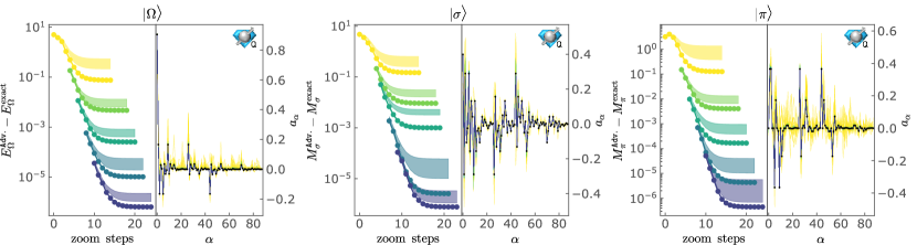
Figure 23: Iterative convergence of the energy, masses and wavefunctions for the three lowest-lying states in the $B=0$ sector of $1+1$D QCD with $N_{f}=2$ and $m=g=L=1$: vacuum (left), $\sigma$-meson (center) and $\pi$-meson (right). Compared to Fig. 7, the exact wavefunctions are used when projecting the Hamiltonian to study the excited states.

Appendix D Quantum Circuits Required for Time Evolution by the Gauge-Field Interaction

This appendix provides more detail about the construction of the quantum circuits which implement the Trotterized time evolution of the chromo-electric terms of the Hamiltonian. It closely follows the presentation in the appendix of Ref. [172]. The four-qubit interaction in $H_{el}$ has the form

$$\sigma^{+}\sigma^{-}\sigma^{-}\sigma^{+}+{\rm h.c.}=\frac{1}{8}(XXXX+XXYY+XYXY-XYYX+YXYX-YXXY+YYXX+YYYY)\ .$$ (53)

Since the 8 Pauli strings are mutually commuting, they can be simultaneously diagonalized by a unitary transformation. The strategy for identifying the quantum circuit(s) to implement this term will be to first change to a basis where every term is diagonal, then apply the diagonal unitaries and finally return back to the computational basis. The GHZ state-preparation circuits, shown in Fig. 12, diagonalize all 8 of the Pauli strings, for example,

$$G^{\dagger}\ (XXXX+YYXX+YXYX-YXXY-XYYX+XYXY+XXYY+YYYY)\ G\ =$$

$$IIZI-ZIZZ-ZZZZ+ZIZI+IZZI-IIZZ-IZZZ+ZZZI\ .$$ (54)

This can be verified by using the identities that are shown in Fig. 24 to simplify the circuits formed by conjugating each Pauli string by $G$. As an example, the diagonalization of $XXYY$ is displayed in Fig. 25.

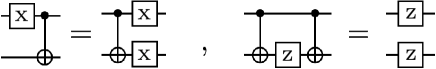
Figure 24: The $X$ and $Z$ circuit identities.

The first equality uses $Y=iZX$ and the second equality uses the $X$ circuit identity to move all $X$s past the CNOTs. The third equality moves the $Z$s past the controls of the CNOTs and uses the $Z$ circuit identity. The other Pauli strings are diagonalized in a similar manner.

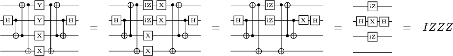
Figure 25: The diagonalization of $XXYY$ via a GHZ state-preparation circuit.

It is also straightforward to show that, for example,

$$G^{\dagger}(IZZI+IZIZ+ZIIZ)G=IZII+IIIZ+ZIII\ .$$ (55)

In general, a $ZZ$ in the computational basis becomes a single $Z$ in the GHZ basis if the state-preparation circuit has a CNOT that connects the original two $Z$s. The two GHZ state-preparation circuits, $G$ and $\tilde{G}$, were chosen so that all $9$ of the $ZZ$ terms in Eq. (7) are mapped to single qubit rotations. Once in the GHZ basis, the diagonal unitaries are performed, e.g., $\exp(-iIZZZ)$. They are arranged to minimize the number of CNOTs required, and the optimal circuit layouts are shown in Fig. 13.

Appendix E Complete Circuits for $N_{f}=1,2$ QCD with $L=1$

This appendix provides the complete set of circuits required to implement one Trotter step for $N_{f}=1$ and $N_{f}=2$ QCD with $L=1$. The composite circuit for $N_{f}=1$ is shown in Fig. 26 where, by ordering $U_{el}$ before $U_{kin}$, the CNOTs highlighted in blue cancel. The composite circuit for $N_{f}=2$ is shown in Fig. 27, where the ordering in the Trotterization is $U_{m}$ followed by $U_{kin}$ and then by $U_{el}$.

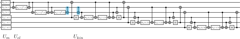
Figure 26: The complete circuit that implements a single Trotter step for $N_{f}=1$ QCD with $L=1$.

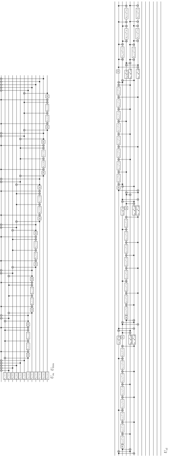
Figure 27: The complete circuit that implements a single Trotter step for $N_{f}=2$ QCD with $L=1$.

Appendix F Energy Decomposition Associated with Time Evolution from the Trivial Vacuum

This appendix shows, in Fig. 28, the time evolution of the decomposition of the expectation value of the Hamiltonian starting with the trivial vacuum at $t=0$ for $N_{f}=2$ QCD with $m=g=L=1$. Notice that the sum of all three terms equals zero for all times as required by energy conservation and that the period of oscillations is the same as the period of the persistence amplitude shown in Fig. 14.

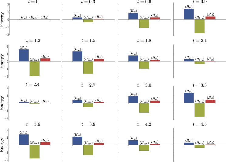
Figure 28: The time evolution of the decomposition of the energy starting from the trivial vacuum starting at $t=0$ for $N_{f}=2$ QCD with $m=g=L=1$.

Appendix G Details on One First-Order Trotter Step of $N_{f}=1$ QCD with $L=1$

This appendix discusses the theoretical expectations for one step of first-order Trotter time evolution for $N_{f}=1$ QCD with $L=1$. The time evolution operator is decomposed into $U_{1}(t)=U_{kin}(t)U_{el}(t)U_{m}(t)$ where the subscript “$1$” is to denote first-order Trotter. Both the trivial vacuum-to-vacuum and trivial vacuum-to-$q_{r}\overline{q}_{r}$ probabilities involve measurements in the computational basis where $U_{m}(t)$ and $U_{el}(t)$ are diagonal and have no effect. Thus, the time-evolution operator is effectively $U_{1}(t)=U_{kin}(t)$, which is exact (no Trotter errors) over a single spatial site. The trivial vacuum-to-vacuum, trivial vacuum-to-$q_{r}\overline{q}_{r}$ and trivial vacuum-to-$B\overline{B}$ probabilities are found to be,

$$\lvert\langle\Omega_{0}\rvert e^{-iH_{kin}t}\lvert\Omega_{0}\rangle\rvert^{2}=\cos^{6}(t/2)\ ,\ \lvert\langle q_{r}\overline{q}_{r}\rvert e^{-iH_{kin}t}\lvert\Omega_{0}\rangle\rvert^{2}=\cos^{4}(t/2)\sin^{2}(t/2)\ ,\ \lvert\langle B\overline{B}\rvert e^{-iH_{kin}t}\lvert\Omega_{0}\rangle\rvert^{2}=\sin^{6}(t/2)\ .$$ (56)

For large periods of the evolution, the wavefunction is dominated by $B\overline{B}$ as shown in Fig. 29. Exact time evolution, on the other hand, has a small probability of $B\overline{B}$ which suggests that detecting $B\overline{B}$ could lead to an additional way to mitigate Trotter errors.

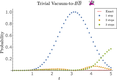
Figure 29: The trivial vacuum-to-$B\overline{B}$ probability for $1+1$D QCD with $m=g=L=1$. Shown are the results obtained from exact exponentiation of the Hamiltonian (dashed red curve) and from the Trotterized implementation with $1$, $2$ and $3$ Trotter steps.

It is interesting that the kinetic term alone favors transitioning the trivial vacuum into color singlets on each site. This same behavior holds for $N_{f}=2$ where the dominant transition is to $\Delta\Delta\overline{\Delta}\overline{\Delta}$.

Appendix H Supplementary Data

This appendix contains the tabulated data used to produce the figures in the text. The splitting between the $\pi$- and $\sigma$-meson is given in Table 9.

$M_{\pi}-M_{\sigma}$
$g$	$L=1$	$L=2$	$g$	$L=1$	$L=2$
0	0.0	0.0	2.1	0.1085	0.09954
0.1	$2.373\times 10^{-6}$	$1.364\times 10^{-6}$	2.2	0.1227	0.1133
0.2	0.0000374	0.00002335	2.3	0.1374	0.1287
0.3	0.0001847	0.0001285	2.4	0.1482	0.1431
0.4	0.0005637	0.0004306	2.5	0.1468	0.1475
0.5	0.001317	0.001066	2.6	0.1321	0.1352
0.6	0.002589	0.002163	2.7	0.1131	0.1156
0.7	0.004508	0.00383	2.8	0.09662	0.09813
0.8	0.007173	0.006158	2.9	0.08372	0.08456
0.9	0.01064	0.009207	3.0	0.07375	0.07422
1.0	0.01493	0.01301	3.1	0.06592	0.06617
1.1	0.02002	0.01755	3.2	0.05961	0.05975
1.2	0.02586	0.02281	3.3	0.05442	0.05448
1.3	0.0324	0.02874	3.4	0.05005	0.05008
1.4	0.03956	0.03529	3.5	0.04631	0.04632
1.5	0.04731	0.04243	3.6	0.04307	0.04306
1.6	0.05562	0.05011	3.7	0.04022	0.04021
1.7	0.0645	0.05837	3.8	0.0377	0.03769
1.8	0.07405	0.06725	3.9	0.03545	0.03543
1.9	0.0844	0.0769	4.0	0.03342	0.0334
2.0	0.0958	0.08755

Table 9: The mass splitting between the $\sigma$- and $\pi$-mesons for $m=1$ and $L=1,2$.

The decomposition of the vacuum energy, hadronic masses and deuteron binding energy is given in Table 10.

Decomposition of the vacuum energy, hadronic masses and deuteron binding energy
	$E_{\Omega}$	$M_{\sigma}$	$M_{\pi}$	$M_{\Delta}$	$B_{\Delta\Delta}$
$\langle H_{m}\rangle$	1.0566	2.056	2.032	2.855	-0.001596
$\langle H_{kin}\rangle$	-2.975	0.1271	0.1425	0.4182	0.002399
$\langle H_{el}\rangle$	0.3374	0.5401	0.5609	-0.03099	-0.0003429

Table 10: The decomposition of vacuum energy ($E_{\Omega}$), the masses of the lightest hadrons ($M_{\sigma}$, $M_{\pi}$ and $M_{\Delta}$) and the deuteron binding energy ($B_{\Delta\Delta}$) into contributions from the mass, kinetic and chromo-electric field terms in the Hamiltonian for $L=2$ and $m=g=1$.

The binding energy of the deuteron is given in Table 11.

$g$	$B_{\Delta\Delta}$	$g$	$B_{\Delta\Delta}$
0	0.0	1.6	0.0005388
0.1	0.00005099	1.7	0.000541
0.2	0.0006768	1.8	0.0005332
0.3	0.002351	1.9	0.0005172
0.4	0.003947	2.0	0.0004948
0.5	0.003905	2.1	0.0004677
0.6	0.002716	2.2	0.0004378
0.7	0.001592	2.3	0.0004063
0.8	0.0009178	2.4	0.0003745
0.9	0.0005902	2.5	0.0003432
1.0	0.0004599	2.6	0.0003129
1.1	0.000429	2.7	0.0002842
1.2	0.000443	2.8	0.0002574
1.3	0.0004727	2.9	0.0002324
1.4	0.0005029	3.0	0.0002095
1.5	0.000526

Table 11: The binding energy of the deuteron, $B_{\Delta\Delta}$, for $m=1$ and $L=2$.

The linear entropy between quarks and antiquarks in the vacuum, the $\sigma$- and $\pi$-meson and the $\Delta$ are given in Table 12.

The linear entropy between quarks and antiquarks
$g$	$\ket{\Omega}$	$\ket{\sigma}$	$\ket{\pi_{I_{3}=1}}$	$\ket{\Delta_{I_{3}=3/2}}$
0.1	0.4668	0.9115	0.7786	0.2698
0.2	0.4617	0.9124	0.7786	0.2663
0.3	0.4532	0.9137	0.7786	0.2605
0.4	0.4416	0.9154	0.7786	0.2527
0.5	0.4271	0.9174	0.7787	0.243
0.6	0.41	0.9194	0.7787	0.2318
0.7	0.3908	0.9214	0.7789	0.2194
0.8	0.3699	0.9232	0.7791	0.206
0.9	0.3478	0.9248	0.7794	0.1921
1.0	0.3248	0.926	0.7798	0.1779
1.1	0.3015	0.9269	0.7803	0.1638
1.2	0.2784	0.9274	0.7811	0.15
1.3	0.2557	0.9277	0.7821	0.1367
1.4	0.2339	0.9277	0.7834	0.1241
1.5	0.213	0.9277	0.7851	0.1123
1.6	0.1935	0.9278	0.7875	0.1014
1.7	0.1752	0.928	0.7906	0.0913
1.8	0.1584	0.9287	0.7949	0.0821
1.9	0.1429	0.93	0.801	0.07375
2.0	0.1288	0.9322	0.8097	0.06622
2.1	0.116	0.9355	0.8225	0.05944
2.2	0.1045	0.9398	0.8416	0.05337
2.3	0.09411	0.9434	0.8675	0.04794
2.4	0.08479	0.9402	0.8889	0.04309
2.5	0.07643	0.9212	0.8731	0.03876
2.6	0.06896	0.8872	0.8209	0.03491
2.7	0.06227	0.8526	0.7729	0.03148
2.8	0.05629	0.8263	0.7414	0.02842
2.9	0.05095	0.8081	0.7216	0.02569
3.0	0.04617	0.7956	0.7086	0.02326
3.1	0.0419	0.7867	0.6994	0.02108
3.2	0.03807	0.7803	0.6928	0.01914
3.3	0.03464	0.7754	0.6877	0.01741
3.4	0.03157	0.7716	0.6837	0.01586
3.5	0.02881	0.7686	0.6805	0.01446
3.6	0.02633	0.7662	0.6779	0.01321
3.7	0.02409	0.7642	0.6757	0.01209
3.8	0.02208	0.7625	0.6739	0.01107
3.9	0.02027	0.7611	0.6723	0.01016
4.0	0.01863	0.7599	0.671	0.009334
4.1	0.01714	0.7588	0.6699	0.008589
4.2	0.0158	0.7579	0.6689	0.007913
4.3	0.01458	0.7572	0.668	0.007301
4.4	0.01347	0.7565	0.6673	0.006745
4.5	0.01246	0.7559	0.6666	0.006239
4.6	0.01154	0.7553	0.666	0.005779
4.7	0.01071	0.7549	0.6655	0.005359
4.8	0.00994	0.7545	0.665	0.004975
4.9	0.00924	0.7541	0.6646	0.004625
5.0	0.0086	0.7538	0.6642	0.004304
5.1	0.008012	0.7535	0.6639	0.004009
5.2	0.007473	0.7532	0.6636	0.003739
5.3	0.006978	0.753	0.6633	0.003491
5.4	0.006522	0.7527	0.6631	0.003263
5.5	0.006101	0.7525	0.6629	0.003052
5.6	0.005714	0.7524	0.6627	0.002858
5.7	0.005356	0.7522	0.6625	0.002679
5.8	0.005026	0.752	0.6623	0.002514
5.9	0.00472	0.7519	0.6621	0.002361
6.0	0.004436	0.7518	0.662	0.002219

Table 12: The linear entropy between quarks and antiquarks in the vacuum, $\ket{\Delta_{I_{3}=3/2}}$, $\ket{\sigma}$ and $\ket{\pi_{I_{3}=1}}$ for $m=L=1$.

The quark occupation (total number of quarks plus antiquarks) in the $\sigma$- and $\pi$-mesons is given in Table 13.

The quark occupation
$g$	$\ket{\sigma}$	$\ket{\pi_{I_{3}=1}}$	$g$	$\ket{\sigma}$	$\ket{\pi_{I_{3}=1}}$
0	2.422	2.422	3.1	5.884	5.915
0.1	2.422	2.422	3.2	5.913	5.936
0.2	2.422	2.422	3.3	5.934	5.95
0.3	2.423	2.422	3.4	5.948	5.961
0.4	2.424	2.423	3.5	5.959	5.968
0.5	2.426	2.423	3.6	5.967	5.974
0.6	2.429	2.423	3.7	5.973	5.979
0.7	2.434	2.424	3.8	5.978	5.982
0.8	2.44	2.425	3.9	5.981	5.985
0.9	2.449	2.427	4.0	5.984	5.988
1.0	2.46	2.43	4.1	5.987	5.989
1.1	2.473	2.434	4.2	5.989	5.991
1.2	2.489	2.439	4.3	5.99	5.992
1.3	2.507	2.445	4.4	5.992	5.993
1.4	2.529	2.454	4.5	5.993	5.994
1.5	2.555	2.466	4.6	5.994	5.995
1.6	2.586	2.483	4.7	5.995	5.996
1.7	2.626	2.505	4.8	5.995	5.996
1.8	2.676	2.537	4.9	5.996	5.997
1.9	2.744	2.584	5.0	5.996	5.997
2.0	2.839	2.655	5.1	5.997	5.997
2.1	2.979	2.769	5.2	5.997	5.998
2.2	3.193	2.966	5.3	5.997	5.998
2.3	3.524	3.318	5.4	5.998	5.998
2.4	4.004	3.911	5.5	5.998	5.998
2.5	4.579	4.66	5.6	5.998	5.999
2.6	5.091	5.249	5.7	5.998	5.999
2.7	5.439	5.577	5.8	5.999	5.999
2.8	5.646	5.743	5.9	5.999	5.999
2.9	5.766	5.832	6.0	5.999	5.999
3.0	5.838	5.883

Table 13: The expectation value of quark occupation in the $\ket{\sigma}$ and $\ket{\pi_{I_{3}=1}}$ for $m=L=1$.

The trivial vacuum-to-vacuum probabilities, as obtained by circ and qiskit, are given in Table 14.

The trivial vacuum-to-vacuum probabilities
$t$	1 Step	2 Steps	3 Steps	5 Steps	10 Steps
0	1	1	1	1	1
0.1	0.9851	0.9852	0.9852	0.9852	0.9852
0.2	0.9417	0.9427	0.9429	0.943	0.943
0.3	0.8733	0.878	0.8789	0.8793	0.8795
0.4	0.7854	0.799	0.8014	0.8027	0.8032
0.5	0.6846	0.7141	0.7193	0.7219	0.723
0.6	0.5779	0.6309	0.6401	0.6447	0.6466
0.7	0.4721	0.5554	0.5697	0.5769	0.5799
0.8	0.3728	0.4914	0.5118	0.522	0.5263
0.9	0.2841	0.4405	0.4678	0.4815	0.4872
1.0	0.2087	0.4032	0.438	0.4556	0.4629
1.1	0.1474	0.3787	0.422	0.4438	0.4529
1.2	0.0999	0.3658	0.4188	0.4454	0.4565
1.3	0.0648	0.3634	0.4275	0.4596	0.4729
1.4	0.0401	0.3699	0.4473	0.4855	0.5012
1.5	0.0235	0.3843	0.4775	0.5225	0.5408
1.6	0.0131	0.4053	0.5174	0.5696	0.5904
1.7	0.0068	0.4316	0.566	0.6252	0.6483
1.8	0.0033	0.4616	0.6218	0.6873	0.712
1.9	0.0015	0.4935	0.6827	0.7529	0.7782
2.0	0.0006	0.5253	0.7458	0.8179	0.8423
2.1	0.0002	0.5546	0.8075	0.8775	0.8992
2.2	0.0001	0.579	0.8634	0.9262	0.9433
2.3	0.0000	0.5965	0.9084	0.9583	0.9691
2.4	0.0000	0.6055	0.9374	0.969	0.9727
2.5	0.0000	0.6055	0.9453	0.9549	0.9518
2.6	0.0000	0.5965	0.9281	0.915	0.907
2.7	0.0000	0.5798	0.8839	0.8513	0.8418
2.8	0.0000	0.5571	0.8129	0.7688	0.7624
2.9	0.0000	0.5305	0.7187	0.6748	0.6766
3.0	0.0000	0.5026	0.6077	0.5778	0.5925
3.1	0.0000	0.4756	0.4886	0.4865	0.5176
3.2	0.0000	0.4518	0.3708	0.408	0.4581
3.3	0.0000	0.4329	0.2629	0.3477	0.4179
3.4	0.0000	0.4204	0.1713	0.3087	0.3991
3.5	0.0000	0.4152	0.0997	0.2921	0.4017
3.6	0.0000	0.4179	0.0488	0.2967	0.424
3.7	0.0000	0.4283	0.0175	0.3196	0.4626
3.8	0.0000	0.4457	0.0035	0.3561	0.5133
3.9	0.0000	0.4689	0.0039	0.4009	0.5714
4.0	0.0000	0.4964	0.0158	0.4485	0.6323
4.1	0.0001	0.5265	0.0363	0.4947	0.6925
4.2	0.0003	0.5578	0.062	0.5373	0.7496
4.3	0.0007	0.5891	0.0893	0.576	0.8015
4.4	0.0017	0.6198	0.1144	0.6125	0.8467
4.5	0.0038	0.6498	0.1339	0.6489	0.8833
4.6	0.0077	0.6794	0.1454	0.687	0.909
4.7	0.0145	0.709	0.148	0.7269	0.9213
4.8	0.0258	0.7389	0.1422	0.7671	0.9177
4.9	0.0436	0.7689	0.1295	0.8042	0.8969
5.0	0.0699	0.7986	0.1125	0.8339	0.8586

Table 14: The trivial vacuum-to-vacuum probabilities for $N_{f}=2$ and $m=g=L=1$. Results are shown for 1, 2, 3, 5 and 10 Trotter steps.

The trivial vacuum-to-$d_{r}\overline{d}_{r}$ probabilities, as obtained by circ and qiskit, are given in Table 15.

The trivial vacuum-to-$d_{r}\overline{d}_{r}$ probabilities
$t$	1 Step	2 Steps	3 Steps	5 Steps	10 Steps
0	0	0	0	0	0
0.1	0.0025	0.0025	0.0025	0.0025	0.0025
0.2	0.0095	0.0093	0.0093	0.0093	0.0093
0.3	0.0199	0.0192	0.0191	0.019	0.019
0.4	0.0323	0.0304	0.0301	0.0299	0.0298
0.5	0.0446	0.0411	0.0405	0.0401	0.04
0.6	0.0553	0.05	0.049	0.0486	0.0483
0.7	0.0629	0.0565	0.0553	0.0546	0.0543
0.8	0.0666	0.0605	0.0591	0.0583	0.058
0.9	0.0663	0.0625	0.061	0.0601	0.0597
1.0	0.0623	0.0629	0.0614	0.0605	0.0601
1.1	0.0554	0.0623	0.0608	0.0598	0.0594
1.2	0.0468	0.0612	0.0597	0.0586	0.058
1.3	0.0374	0.0599	0.0581	0.0567	0.0561
1.4	0.0284	0.0585	0.0561	0.0543	0.0535
1.5	0.0204	0.0569	0.0537	0.0512	0.0501
1.6	0.0139	0.0552	0.0505	0.0472	0.0458
1.7	0.0088	0.0531	0.0464	0.0422	0.0403
1.8	0.0053	0.0505	0.0414	0.0361	0.0339
1.9	0.0029	0.0473	0.0353	0.029	0.0265
2.0	0.0015	0.0434	0.0283	0.0213	0.0188
2.1	0.0007	0.039	0.0208	0.0137	0.0113
2.2	0.0003	0.0341	0.0134	0.007	0.0051
2.3	0.0001	0.0291	0.0069	0.0022	0.0012
2.4	0.0000	0.0239	0.0024	0.0005	0.0006
2.5	0.0000	0.0189	0.0008	0.0025	0.0036
2.6	0.0000	0.0142	0.0031	0.0085	0.0105
2.7	0.0000	0.0099	0.0098	0.0183	0.0206
2.8	0.0000	0.0061	0.0204	0.0308	0.0326
2.9	0.0000	0.0031	0.0339	0.0444	0.0452
3.0	0.0000	0.0011	0.0482	0.0574	0.0568
3.1	0.0000	0.0001	0.061	0.0686	0.0663
3.2	0.0000	0.0002	0.0701	0.0768	0.073
3.3	0.0000	0.0012	0.0741	0.0818	0.0766
3.4	0.0000	0.003	0.0728	0.0834	0.0769
3.5	0.0000	0.0052	0.0673	0.082	0.0741
3.6	0.0000	0.0074	0.0594	0.0777	0.0687
3.7	0.0000	0.0094	0.0508	0.0712	0.0613
3.8	0.0000	0.0108	0.0429	0.0632	0.0527
3.9	0.0000	0.0117	0.0366	0.0546	0.0439
4.0	0.0001	0.0121	0.0315	0.0467	0.0356
4.1	0.0003	0.0122	0.0275	0.0401	0.0283
4.2	0.0008	0.0121	0.024	0.0351	0.0221
4.3	0.0017	0.0121	0.0209	0.0316	0.0167
4.4	0.0033	0.0123	0.0183	0.0289	0.012
4.5	0.0058	0.0126	0.0166	0.0262	0.008
4.6	0.0096	0.013	0.0162	0.0229	0.0049
4.7	0.0149	0.0132	0.0169	0.0188	0.003
4.8	0.0217	0.0131	0.0185	0.0142	0.003
4.9	0.0299	0.0127	0.0207	0.0097	0.0052
5.0	0.039	0.0119	0.0228	0.0062	0.0099

Table 15: The trivial vacuum-to-$d_{r}\overline{d}_{r}$ probabilities for $N_{f}=2$ and $m=g=L=1$. Results are shown for 1, 2, 3, 5 and 10 Trotter steps.

The required $N$_Trott for a $\epsilon_{{\rm Trott}}<0.1$ in the trivial vacuum-to-vacuum probability is given in Table 16.

Required number of Trotter steps, $N$Trott
$t$	$N$Trott	$t$	$N$Trott	$t$	$N$Trott	$t$	$N$Trott	$t$	$N$Trott	$t$	$N$Trott	$t$	$N$Trott	$t$	$N$Trott
0	1	25	95	50	271	75	521	100	740	125	1080	150	1417	175	1967
0.5	1	25.5	95	50.5	271	75.5	521	100.5	740	125.5	1080	150.5	1598	175.5	1967
1	3	26	103	51	271	76	521	101	740	126	1113	151	1598	176	1967
1.5	4	26.5	103	51.5	302	76.5	521	101.5	740	126.5	1113	151.5	1598	176.5	1967
2	4	27	114	52	302	77	521	102	794	127	1113	152	1598	177	1967
2.5	4	27.5	114	52.5	302	77.5	521	102.5	794	127.5	1224	152.5	1598	177.5	1967
3	4	28	114	53	302	78	521	103	868	128	1224	153	1598	178	1967
3.5	10	28.5	121	53.5	302	78.5	521	103.5	868	128.5	1224	153.5	1598	178.5	1967
4	10	29	130	54	302	79	535	104	868	129	1224	154	1598	179	2023
4.5	10	29.5	130	54.5	335	79.5	535	104.5	868	129.5	1224	154.5	1598	179.5	2023
5	10	30	130	55	335	80	597	105	868	130	1224	155	1598	180	2023
5.5	10	30.5	130	55.5	335	80.5	597	105.5	868	130.5	1224	155.5	1598	180.5	2023
6	19	31	130	56	335	81	597	106	868	131	1224	156	1598	181	2023
6.5	19	31.5	159	56.5	335	81.5	597	106.5	868	131.5	1224	156.5	1598	181.5	2023
7	19	32	159	57	363	82	597	107	868	132	1224	157	1598	182	2023
7.5	19	32.5	159	57.5	363	82.5	597	107.5	868	132.5	1224	157.5	1598	182.5	2023
8	19	33	159	58	363	83	597	108	868	133	1224	158	1598	183	2023
8.5	27	33.5	159	58.5	363	83.5	597	108.5	868	133.5	1224	158.5	1598	183.5	2023
9	27	34	167	59	363	84	597	109	896	134	1224	159	1598	184	2023
9.5	27	34.5	167	59.5	363	84.5	613	109.5	896	134.5	1224	159.5	1598	184.5	2023
10	27	35	167	60	363	85	613	110	896	135	1224	160	1598	185	2137
10.5	29	35.5	167	60.5	363	85.5	613	110.5	896	135.5	1224	160.5	1598	185.5	2137
11	34	36	167	61	363	86	631	111	896	136	1224	161	1598	186	2137
11.5	34	36.5	167	61.5	370	86.5	631	111.5	896	136.5	1279	161.5	1598	186.5	2137
12	34	37	167	62	370	87	631	112	896	137	1279	162	1719	187	2137
12.5	34	37.5	182	62.5	370	87.5	631	112.5	896	137.5	1279	162.5	1719	187.5	2203
13	42	38	182	63	397	88	631	113	896	138	1279	163	1719	188	2203
13.5	42	38.5	186	63.5	397	88.5	631	113.5	975	138.5	1279	163.5	1719	188.5	2203
14	42	39	186	64	397	89	650	114	975	139	1356	164	1719	189	2203
14.5	42	39.5	186	64.5	397	89.5	650	114.5	975	139.5	1356	164.5	1747	189.5	2203
15	42	40	197	65	397	90	650	115	975	140	1356	165	1747	190	2203
15.5	51	40.5	197	65.5	397	90.5	692	115.5	975	140.5	1356	165.5	1747	190.5	2203
16	51	41	197	66	453	91	692	116	1000	141	1356	166	1747	191	2203
16.5	51	41.5	197	66.5	453	91.5	705	116.5	1000	141.5	1356	166.5	1747	191.5	2203
17	51	42	197	67	453	92	705	117	1000	142	1356	167	1747	192	2203
17.5	67	42.5	197	67.5	453	92.5	705	117.5	1000	142.5	1356	167.5	1798	192.5	2203
18	67	43	248	68	453	93	707	118	1000	143	1356	168	1798	193	2203
18.5	67	43.5	248	68.5	475	93.5	707	118.5	1000	143.5	1356	168.5	1798	193.5	2203
19	67	44	248	69	475	94	707	119	1000	144	1356	169	1798	194	2203
19.5	67	44.5	248	69.5	475	94.5	707	119.5	1000	144.5	1417	169.5	1798	194.5	2203
20	85	45	248	70	475	95	707	120	1000	145	1417	170	1798	195	2203
20.5	85	45.5	264	70.5	475	95.5	707	120.5	1000	145.5	1417	170.5	1798	195.5	2203
21	85	46	264	71	475	96	707	121	1000	146	1417	171	1798	196	2203
21.5	85	46.5	264	71.5	475	96.5	707	121.5	1075	146.5	1417	171.5	1798	196.5	2273
22	85	47	264	72	475	97	707	122	1075	147	1417	172	1798	197	2273
22.5	95	47.5	264	72.5	475	97.5	735	122.5	1075	147.5	1417	172.5	1798	197.5	2273
23	95	48	264	73	475	98	735	123	1075	148	1417	173	1798	198	2273
23.5	95	48.5	264	73.5	475	98.5	740	123.5	1075	148.5	1417	173.5	1967	198.5	2273
24	95	49	264	74	475	99	740	124	1075	149	1417	174	1967	199	2352
24.5	95	49.5	264	74.5	521	99.5	740	124.5	1075	149.5	1417	174.5	1967	199.5	2352

Table 16: The required $N$_Trott for a $\epsilon_{{\rm Trott}}<0.1$ in the trivial vacuum-to-vacuum probability.

The required $N$_Trott for a $\epsilon_{{\rm Trott}}<0.1$ in the trivial vacuum-to-$d_{r}\overline{d}_{r}$ probability is given in Table 17.

Required number of Trotter steps, $N$Trott
$t$	$N$Trott	$t$	$N$Trott	$t$	$N$Trott	$t$	$N$Trott
0	1	25	243	50	945	75	1706
0.5	2	25.5	337	50.5	945	75.5	1706
1	2	26	337	51	945	76	1739
1.5	3	26.5	337	51.5	945	76.5	1739
2	7	27	337	52	945	77	1739
2.5	10	27.5	337	52.5	945	77.5	1739
3	10	28	337	53	945	78	1739
3.5	10	28.5	337	53.5	945	78.5	1739
4	12	29	337	54	945	79	1739
4.5	24	29.5	337	54.5	945	79.5	1739
5	24	30	337	55	945	80	1739
5.5	24	30.5	337	55.5	945	80.5	1739
6	24	31	337	56	945	81	1739
6.5	32	31.5	337	56.5	945	81.5	1739
7	32	32	384	57	945	82	1739
7.5	32	32.5	384	57.5	1168	82.5	1739
8	32	33	384	58	1168	83	2064
8.5	33	33.5	384	58.5	1168	83.5	2064
9	72	34	384	59	1168	84	2064
9.5	72	34.5	709	59.5	1168	84.5	2064
10	72	35	709	60	1285	85	2064
10.5	72	35.5	709	60.5	1285	85.5	2064
11	72	36	709	61	1285	86	2064
11.5	98	36.5	709	61.5	1285	86.5	2064
12	98	37	709	62	1285	87	2064
12.5	98	37.5	709	62.5	1285	87.5	2064
13	98	38	709	63	1285	88	2064
13.5	98	38.5	709	63.5	1285	88.5	2064
14	148	39	709	64	1285	89	2064
14.5	148	39.5	709	64.5	1285	89.5	2064
15	148	40	709	65	1285	90	2064
15.5	148	40.5	709	65.5	1285	90.5	2064
16	148	41	709	66	1285	91	2064
16.5	148	41.5	709	66.5	1285	91.5	2064
17	148	42	709	67	1285	92	2064
17.5	148	42.5	709	67.5	1285	92.5	2064
18	148	43	709	68	1285	93	2064
18.5	148	43.5	709	68.5	1285	93.5	2064
19	148	44	709	69	1285	94	2064
19.5	148	44.5	709	69.5	1285	94.5	2590
20	148	45	709	70	1285	95	2590
20.5	233	45.5	709	70.5	1285	95.5	2590
21	233	46	709	71	1285	96	2590
21.5	233	46.5	709	71.5	1706	96.5	2590
22	233	47	709	72	1706	97	2590
22.5	233	47.5	709	72.5	1706	97.5	2590
23	243	48	709	73	1706	98	2590
23.5	243	48.5	945	73.5	1706	98.5	2590
24	243	49	945	74	1706	99	2780
24.5	243	49.5	945	74.5	1706	99.5	2780

Table 17: The required $N$_Trott for a $\epsilon_{{\rm Trott}}<0.1$ in the trivial vacuum-to-$d_{r}\overline{d}_{r}$ probability.

The decomposition of the energy, starting from trivial vacuum at $t=0$, is given in Table 18.

Decomposition of the energy starting from the trivial vacuum
$t$	$\langle H_{m}\rangle$	$\langle H_{kin}\rangle$	$\langle H_{el}\rangle$
0	0	0	0
0.3	0.254	-0.3369	0.08281
0.6	0.8455	-1.104	0.2584
0.9	1.393	-1.781	0.3879
1.2	1.575	-1.974	0.3997
1.5	1.31	-1.625	0.3151
1.8	0.769	-0.9532	0.1842
2.1	0.2684	-0.3282	0.05983
2.4	0.1081	-0.1256	0.01747
2.7	0.3939	-0.5129	0.119
3.0	0.9349	-1.245	0.31
3.3	1.359	-1.788	0.4285
3.6	1.401	-1.788	0.3873
3.9	1.079	-1.335	0.2565
4.2	0.6237	-0.7542	0.1305
4.5	0.3094	-0.3586	0.0492

Table 18: Decomposition of the energy starting from the trivial vacuum at $t=0$.

The trivial vacuum to $B\overline{B}$ probabilities are given in Table 19.

Trivial vacuum to $B\overline{B}$ probability
$t$	1 Step	2 Steps	3 Steps	Exact
0	0	0	0	0
0.1	0.0000	0.0000	0.0000	0.0000
0.2	0.0000	0.0000	0.0000	0.0000
0.3	0.0000	0.0000	0.0000	0.0000
0.4	0.0001	0.0001	0.0001	0.0001
0.5	0.0002	0.0002	0.0002	0.0002
0.6	0.0007	0.0005	0.0005	0.0005
0.7	0.0016	0.0011	0.001	0.001
0.8	0.0035	0.0021	0.0019	0.0018
0.9	0.0068	0.0036	0.0032	0.0029
1.0	0.0121	0.0055	0.0047	0.0042
1.1	0.0204	0.0079	0.0064	0.0055
1.2	0.0324	0.0104	0.0081	0.0067
1.3	0.0491	0.013	0.0095	0.0075
1.4	0.0715	0.0154	0.0105	0.0079
1.5	0.1003	0.0175	0.0109	0.0078
1.6	0.1363	0.0192	0.0108	0.0072
1.7	0.1798	0.0206	0.0101	0.0062
1.8	0.231	0.0218	0.0092	0.0052
1.9	0.2897	0.023	0.008	0.0041
2.0	0.355	0.0241	0.0069	0.0033
2.1	0.426	0.0252	0.0059	0.0025
2.2	0.501	0.026	0.005	0.002
2.3	0.5783	0.0263	0.0042	0.0015
2.4	0.6555	0.0257	0.0036	0.0011
2.5	0.7304	0.0239	0.003	0.0007
2.6	0.8003	0.0208	0.0026	0.0004
2.7	0.8629	0.0166	0.0024	0.0001
2.8	0.9158	0.0116	0.0025	0.0000
2.9	0.9571	0.0066	0.0029	0.0000
3.0	0.9851	0.0025	0.0036	0.0002
3.1	0.9987	0.0002	0.0045	0.0005
3.2	0.9974	0.0005	0.0057	0.0008
3.3	0.9813	0.0037	0.007	0.0011
3.4	0.951	0.01	0.0087	0.0014
3.5	0.9077	0.0189	0.0111	0.0016
3.6	0.853	0.0295	0.0148	0.0019
3.7	0.789	0.0409	0.0205	0.0023
3.8	0.7181	0.0517	0.0293	0.0027
3.9	0.6427	0.061	0.042	0.0032
4.0	0.5652	0.0677	0.0592	0.0036
4.1	0.4882	0.0714	0.0814	0.004
4.2	0.4137	0.0719	0.1085	0.0043
4.3	0.3436	0.0693	0.14	0.0045
4.4	0.2793	0.0641	0.1749	0.0046
4.5	0.2219	0.057	0.2117	0.0047
4.6	0.172	0.0488	0.2489	0.0049
4.7	0.1297	0.0401	0.2848	0.005
4.8	0.095	0.0317	0.3178	0.0051
4.9	0.0673	0.024	0.3464	0.0051
5.0	0.0459	0.0174	0.3695	0.0048

Table 19: Trivial vacuum to $B\overline{B}$ probability for $m=g=L=N_{f}=1$.

References

- [1] S. Glashow, Partial Symmetries of Weak Interactions, Nucl. Phys. 22 (1961) 579.
- [2] P.W. Higgs, Broken Symmetries and the Masses of Gauge Bosons, Phys. Rev. Lett. 13 (1964) 508.
- [3] S. Weinberg, A Model of Leptons, Phys. Rev. Lett. 19 (1967) 1264.
- [4] A. Salam, Weak and Electromagnetic Interactions, Conf. Proc. C 680519 (1968) 367.
- [5] H. Politzer, Reliable Perturbative Results for Strong Interactions?, Phys. Rev. Lett. 30 (1973) 1346.
- [6] D.J. Gross and F. Wilczek, Ultraviolet Behavior of Nonabelian Gauge Theories, Phys. Rev. Lett. 30 (1973) 1343.
- [7] S. Lloyd, Universal quantum simulators, Science 273 (1996) 1073.
- [8] R. Landauer, Irreversibility and heat generation in the computing process, IBM Journal of Research and Development 5 (1961) 183.
- [9] C.H. Bennett, Logical reversibility of computation, IBM Journal of Research and Development 17 (1973) 525.
- [10] P. Benioff, The computer as a physical system: A microscopic quantum mechanical hamiltonian model of computers as represented by turing machines, Journal of Statistical Physics 22 (1980) 563.
- [11] Y. Manin, Computable and Uncomputable, Sovetskoye Radio, Moscow” 128 (1980) .
- [12] R.P. Feynman, Simulating physics with computers, International Journal of Theoretical Physics 21 (1982) 467.
- [13] E. Fredkin and T. Toffoli, Conservative logic, International Journal of Theoretical Physics 21 (1982) 219.
- [14] R.P. Feynman, Quantum mechanical computers, Foundations of Physics 16 (1986) 507.
- [15] R. Landauer, Information is physical, Physics Today 44 (1991) 23.
- [16] C.P. Williams, ed., Quantum Computing and Quantum Communications, First NASA International Conference, QCQC’98, Palm Springs, California, USA, February 17-20, 1998, Selected Papers, vol. 1509 of Lecture Notes in Computer Science, Springer, 1998. 10.1007/3-540-49208-9.
- [17] J. Preskill, Quantum computing 40 years later, 2106.10522.
- [18] N. Klco, A. Roggero and M.J. Savage, Standard model physics and the digital quantum revolution: thoughts about the interface, Rept. Prog. Phys. 85 (2022) 064301 [2107.04769].
- [19] C.W. Bauer, Z. Davoudi, A.B. Balantekin, T. Bhattacharya, M. Carena, W.A. de Jong et al., Quantum Simulation for High Energy Physics, 2204.03381.
- [20] J. Preskill, Quantum Computing in the NISQ era and beyond, Quantum 2 (2018) 79 [1801.00862].
- [21] P. Hauke, D. Marcos, M. Dalmonte and P. Zoller, Quantum simulation of a lattice Schwinger model in a chain of trapped ions, Phys. Rev. X 3 (2013) 041018 [1306.2162].
- [22] M.C. Bañuls, K. Cichy, K. Jansen and J.I. Cirac, The mass spectrum of the Schwinger model with Matrix Product States, JHEP 11 (2013) 158 [1305.3765].
- [23] E. Zohar, A. Farace, B. Reznik and J.I. Cirac, Digital lattice gauge theories, Phys. Rev. A 95 (2017) 023604 [1607.08121].
- [24] C. Muschik, M. Heyl, E. Martinez, T. Monz, P. Schindler, B. Vogell et al., U(1) Wilson lattice gauge theories in digital quantum simulators, New J. Phys. 19 (2017) 103020 [1612.08653].
- [25] E.A. Martinez et al., Real-time dynamics of lattice gauge theories with a few-qubit quantum computer, Nature 534 (2016) 516 [1605.04570].
- [26] B. Buyens, J. Haegeman, F. Hebenstreit, F. Verstraete and K. Van Acoleyen, Real-time simulation of the Schwinger effect with Matrix Product States, Phys. Rev. D 96 (2017) 114501 [1612.00739].
- [27] M.C. Bañuls, K. Cichy, K. Jansen and H. Saito, Chiral condensate in the Schwinger model with Matrix Product Operators, Phys. Rev. D 93 (2016) 094512 [1603.05002].
- [28] D. González-Cuadra, E. Zohar and J.I. Cirac, Quantum Simulation of the Abelian-Higgs Lattice Gauge Theory with Ultracold Atoms, New J. Phys. 19 (2017) 063038 [1702.05492].
- [29] E.F. Dumitrescu, A.J. McCaskey, G. Hagen, G.R. Jansen, T.D. Morris, T. Papenbrock et al., Cloud Quantum Computing of an Atomic Nucleus, Phys. Rev. Lett. 120 (2018) 210501 [1801.03897].
- [30] N. Klco, E.F. Dumitrescu, A.J. McCaskey, T.D. Morris, R.C. Pooser, M. Sanz et al., Quantum-classical computation of schwinger model dynamics using quantum computers, Phys. Rev. A 98 (2018) 032331 [1803.03326].
- [31] H.-H. Lu, N. Klco, J.M. Lukens, T.D. Morris, A. Bansal, A. Ekström et al., Simulations of subatomic many-body physics on a quantum frequency processor, Phys. Rev. A 100 (2019) 012320.
- [32] D.B. Kaplan and J.R. Stryker, Gauss’s law, duality, and the Hamiltonian formulation of U(1) lattice gauge theory, Phys. Rev. D 102 (2020) 094515 [1806.08797].
- [33] J.R. Stryker, Oracles for Gauss’s law on digital quantum computers, Phys. Rev. A 99 (2019) 042301 [1812.01617].
- [34] K. Yeter-Aydeniz, E.F. Dumitrescu, A.J. McCaskey, R.S. Bennink, R.C. Pooser and G. Siopsis, Scalar Quantum Field Theories as a Benchmark for Near-Term Quantum Computers, Phys. Rev. A 99 (2019) 032306 [1811.12332].
- [35] N. Klco, M.J. Savage and J.R. Stryker, SU(2) non-Abelian gauge field theory in one dimension on digital quantum computers, Phys. Rev. D 101 (2020) 074512 [1908.06935].
- [36] A. Avkhadiev, P.E. Shanahan and R.D. Young, Accelerating Lattice Quantum Field Theory Calculations via Interpolator Optimization Using Noisy Intermediate-Scale Quantum Computing, Phys. Rev. Lett. 124 (2020) 080501 [1908.04194].
- [37] C.W. Bauer, W.A. de Jong, B. Nachman and D. Provasoli, Quantum Algorithm for High Energy Physics Simulations, Phys. Rev. Lett. 126 (2021) 062001 [1904.03196].
- [38] N. Klco and M.J. Savage, Minimally entangled state preparation of localized wave functions on quantum computers, Phys. Rev. A 102 (2020) 012612 [1904.10440].
- [39] N. Klco and M.J. Savage, Systematically Localizable Operators for Quantum Simulations of Quantum Field Theories, Phys. Rev. A 102 (2020) 012619 [1912.03577].
- [40] M.C. Bañuls et al., Simulating Lattice Gauge Theories within Quantum Technologies, Eur. Phys. J. D 74 (2020) 165 [1911.00003].
- [41] D. Luo, J. Shen, M. Highman, B.K. Clark, B. DeMarco, A.X. El-Khadra et al., Framework for simulating gauge theories with dipolar spin systems, Phys. Rev. A 102 (2020) 032617 [1912.11488].
- [42] L. Funcke, K. Jansen and S. Kühn, Topological vacuum structure of the Schwinger model with matrix product states, Phys. Rev. D 101 (2020) 054507 [1908.00551].
- [43] Z. Davoudi, M. Hafezi, C. Monroe, G. Pagano, A. Seif and A. Shaw, Towards analog quantum simulations of lattice gauge theories with trapped ions, Phys. Rev. Res. 2 (2020) 023015 [1908.03210].
- [44] G. Magnifico, M. Dalmonte, P. Facchi, S. Pascazio, F.V. Pepe and E. Ercolessi, Real Time Dynamics and Confinement in the Schwinger-Weyl lattice model for 1+1 QED, Quantum 4 (2020) 281 [1909.04821].
- [45] C. Mishra, S. Thompson, R. Pooser and G. Siopsis, Quantum Computation of the Massive Thirring Model, Quantum Sci. Technol. 5 (2020) 035010 [1912.07767].
- [46] O. Shehab, K.A. Landsman, Y. Nam, D. Zhu, N.M. Linke, M.J. Keesan et al., Toward convergence of effective field theory simulations on digital quantum computers, Phys. Rev. A 100 (2019) 062319 [1904.04338].
- [47] B. Yang, H. Sun, R. Ott, H.-Y. Wang, T.V. Zache, J.C. Halimeh et al., Observation of gauge invariance in a 71-site bose–hubbard quantum simulator, Nature 587 (2020) 392–396 [2003.08945].
- [48] D.E. Kharzeev and Y. Kikuchi, Real-time chiral dynamics from a digital quantum simulation, Phys. Rev. Research 2 (2020) 023342 [2001.00698].
- [49] A.F. Shaw, P. Lougovski, J.R. Stryker and N. Wiebe, Quantum Algorithms for Simulating the Lattice Schwinger Model, Quantum 4 (2020) 306 [2002.11146].
- [50] A. Ciavarella, N. Klco and M.J. Savage, Trailhead for quantum simulation of SU(3) Yang-Mills lattice gauge theory in the local multiplet basis, Phys. Rev. D 103 (2021) 094501 [2101.10227].
- [51] J.C. Halimeh, H. Lang, J. Mildenberger, Z. Jiang and P. Hauke, Gauge-Symmetry Protection Using Single-Body Terms, PRX Quantum 2 (2021) 040311 [2007.00668].
- [52] J.C. Halimeh, V. Kasper and P. Hauke, Fate of Lattice Gauge Theories Under Decoherence, 2009.07848.
- [53] M. Van Damme, J.C. Halimeh and P. Hauke, Gauge-Symmetry Violation Quantum Phase Transition in Lattice Gauge Theories, 2010.07338.
- [54] J.F. Haase, L. Dellantonio, A. Celi, D. Paulson, A. Kan, K. Jansen et al., A resource efficient approach for quantum and classical simulations of gauge theories in particle physics, Quantum 5 (2021) 393 [2006.14160].
- [55] K. Yeter-Aydeniz, G. Siopsis and R.C. Pooser, Scattering in the Ising model with the quantum Lanczos algorithm, New J. Phys. 23 (2021) 043033 [2008.08763].
- [56] Z. Davoudi, N.M. Linke and G. Pagano, Toward simulating quantum field theories with controlled phonon-ion dynamics: A hybrid analog-digital approach, Phys. Rev. Research 3 (2021) 043072 [2104.09346].
- [57] S. A Rahman, R. Lewis, E. Mendicelli and S. Powell, SU(2) lattice gauge theory on a quantum annealer, Phys. Rev. D 104 (2021) 034501 [2103.08661].
- [58] T.V. Zache, N. Mueller, J.T. Schneider, F. Jendrzejewski, J. Berges and P. Hauke, Dynamical topological transitions in the massive schwinger model with a term, Phys. Rev. Lett. 122 (2019) 050403.
- [59] J.R. Stryker, Shearing approach to gauge invariant Trotterization, 2105.11548.
- [60] M. Aidelsburger, L. Barbiero, A. Bermudez, T. Chanda, A. Dauphin, D. González-Cuadra et al., Cold atoms meet lattice gauge theory, Phil. Trans. Roy. Soc. Lond. A 380 (2021) 20210064 [2106.03063].
- [61] C.W. Bauer, M. Freytsis and B. Nachman, Simulating Collider Physics on Quantum Computers Using Effective Field Theories, Phys. Rev. Lett. 127 (2021) 212001 [2102.05044].
- [62] M. Van Damme, J. Mildenberger, F. Grusdt, P. Hauke and J.C. Halimeh, Suppressing nonperturbative gauge errors in the thermodynamic limit using local pseudogenerators, 2110.08041.
- [63] J.C. Halimeh, L. Homeier, C. Schweizer, M. Aidelsburger, P. Hauke and F. Grusdt, Stabilizing Lattice Gauge Theories Through Simplified Local Pseudo Generators, Phys. Rev. Res. 4 (2022) 033120 [2108.02203].
- [64] J. Knaute and P. Hauke, Relativistic meson spectra on ion-trap quantum simulators, Phys. Rev. A 105 (2022) 022616 [2107.09071].
- [65] J.C. Halimeh, H. Lang and P. Hauke, Gauge protection in non-abelian lattice gauge theories, New J. Phys. 24 (2022) 033015 [2106.09032].
- [66] S. Thompson and G. Siopsis, Quantum computation of phase transition in the massive Schwinger model, Quantum Sci. Technol. 7 (2022) 035001 [2110.13046].
- [67] K. Yeter-Aydeniz, E. Moschandreou and G. Siopsis, Quantum imaginary-time evolution algorithm for quantum field theories with continuous variables, Phys. Rev. A 105 (2022) 012412 [2107.00791].
- [68] K. Yeter-Aydeniz, S. Bangar, G. Siopsis and R.C. Pooser, Collective neutrino oscillations on a quantum computer, Quant. Inf. Proc. 21 (2022) 84 [2104.03273].
- [69] L. Funcke, T. Hartung, K. Jansen, S. Kühn, M. Schneider, P. Stornati et al., Towards quantum simulations in particle physics and beyond on noisy intermediate-scale quantum devices, Phil. Trans. A. Math. Phys. Eng. Sci. 380 (2021) 20210062 [2110.03809].
- [70] J. Zhang, R. Ferguson, S. Kühn, J.F. Haase, C.M. Wilson, K. Jansen et al., Simulating gauge theories with variational quantum eigensolvers in superconducting microwave cavities, 2108.08248.
- [71] S. A Rahman, R. Lewis, E. Mendicelli and S. Powell, Self-mitigating Trotter circuits for SU(2) lattice gauge theory on a quantum computer, Phys. Rev. D 106 (2022) 074502 [2205.09247].
- [72] P. Deliyannis, J. Sud, D. Chamaki, Z. Webb-Mack, C.W. Bauer and B. Nachman, Improving Quantum Simulation Efficiency of Final State Radiation with Dynamic Quantum Circuits, Phys. Rev. D 106 (2022) 036007 [2203.10018].
- [73] C.W. Bauer and D.M. Grabowska, Efficient representation for simulating U(1) gauge theories on digital quantum computers at all values of the coupling, Phys. Rev. D 107 (2023) L031503 [2111.08015].
- [74] M. Illa and M.J. Savage, Basic elements for simulations of standard-model physics with quantum annealers: Multigrid and clock states, Phys. Rev. A 106 (2022) 052605 [2202.12340].
- [75] J. Mildenberger, W. Mruczkiewicz, J.C. Halimeh, Z. Jiang and P. Hauke, Probing confinement in a lattice gauge theory on a quantum computer, 2203.08905.
- [76] A. Milsted, J. Liu, J. Preskill and G. Vidal, Collisions of false-vacuum bubble walls in a quantum spin chain, PRX Quantum 3 (2022) 020316 [2012.07243].
- [77] N. Klco, E.F. Dumitrescu, A.J. McCaskey, T.D. Morris, R.C. Pooser, M. Sanz et al., Quantum-classical computation of Schwinger model dynamics using quantum computers, Phys. Rev. A 98 (2018) 032331 [1803.03326].
- [78] C. Kokail et al., Self-verifying variational quantum simulation of lattice models, Nature 569 (2019) 355 [1810.03421].
- [79] N.H. Nguyen, M.C. Tran, Y. Zhu, A.M. Green, C.H. Alderete, Z. Davoudi et al., Digital Quantum Simulation of the Schwinger Model and Symmetry Protection with Trapped Ions, PRX Quantum 3 (2022) 020324 [2112.14262].
- [80] E. Zohar and B. Reznik, Confinement and lattice QED electric flux-tubes simulated with ultracold atoms, Phys. Rev. Lett. 107 (2011) 275301 [1108.1562].
- [81] E. Zohar, J.I. Cirac and B. Reznik, Simulating Compact Quantum Electrodynamics with ultracold atoms: Probing confinement and nonperturbative effects, Phys. Rev. Lett. 109 (2012) 125302 [1204.6574].
- [82] L. Tagliacozzo, A. Celi, A. Zamora and M. Lewenstein, Optical Abelian Lattice Gauge Theories, Annals Phys. 330 (2013) 160 [1205.0496].
- [83] E. Zohar, J.I. Cirac and B. Reznik, Simulating (2+1)-Dimensional Lattice QED with Dynamical Matter Using Ultracold Atoms, Phys. Rev. Lett. 110 (2013) 055302 [1208.4299].
- [84] U.-J. Wiese, Ultracold Quantum Gases and Lattice Systems: Quantum Simulation of Lattice Gauge Theories, Annalen Phys. 525 (2013) 777 [1305.1602].
- [85] D. Marcos, P. Widmer, E. Rico, M. Hafezi, P. Rabl, U.J. Wiese et al., Two-dimensional Lattice Gauge Theories with Superconducting Quantum Circuits, Annals Phys. 351 (2014) 634 [1407.6066].
- [86] Y. Kuno, K. Kasamatsu, Y. Takahashi, I. Ichinose and T. Matsui, Real-time dynamics and proposal for feasible experiments of lattice gauge–Higgs model simulated by cold atoms, New J. Phys. 17 (2015) 063005 [1412.7605].
- [87] A. Bazavov, Y. Meurice, S.-W. Tsai, J. Unmuth-Yockey and J. Zhang, Gauge-invariant implementation of the Abelian Higgs model on optical lattices, Phys. Rev. D 92 (2015) 076003 [1503.08354].
- [88] V. Kasper, F. Hebenstreit, M. Oberthaler and J. Berges, Schwinger pair production with ultracold atoms, Phys. Lett. B 760 (2016) 742 [1506.01238].
- [89] G.K. Brennen, G. Pupillo, E. Rico, T.M. Stace and D. Vodola, Loops and Strings in a Superconducting Lattice Gauge Simulator, Phys. Rev. Lett. 117 (2016) 240504 [1512.06565].
- [90] Y. Kuno, S. Sakane, K. Kasamatsu, I. Ichinose and T. Matsui, Atomic quantum simulation of a three-dimensional U(1) gauge-Higgs model, Phys. Rev. A 94 (2016) 063641 [1605.02502].
- [91] V. Kasper, F. Hebenstreit, F. Jendrzejewski, M.K. Oberthaler and J. Berges, Implementing quantum electrodynamics with ultracold atomic systems, New J. Phys. 19 (2017) 023030 [1608.03480].
- [92] R. Ott, T.V. Zache, F. Jendrzejewski and J. Berges, Scalable Cold-Atom Quantum Simulator for Two-Dimensional QED, Phys. Rev. Lett. 127 (2021) 130504 [2012.10432].
- [93] D. Paulson et al., Towards simulating 2D effects in lattice gauge theories on a quantum computer, PRX Quantum 2 (2021) 030334 [2008.09252].
- [94] A. Kan, L. Funcke, S. Kühn, L. Dellantonio, J. Zhang, J.F. Haase et al., Investigating a 3+1D Topological -Term in the Hamiltonian Formulation of Lattice Gauge Theories for Quantum and Classical Simulations, Phys. Rev. D 104 (2021) 034504 [2105.06019].
- [95] K.G. Wilson, T.S. Walhout, A. Harindranath, W.-M. Zhang, R.J. Perry and S.D. Glazek, Nonperturbative QCD: A Weak coupling treatment on the light front, Phys. Rev. D 49 (1994) 6720 [hep-th/9401153].
- [96] T. Heinzl, Hamiltonian formulations of Yang-Mills quantum theory and the Gribov problem, in 5th Meeting on Light Cone Quantization and Nonperturbative QCD, 6, 1995 [hep-th/9604018].
- [97] J.B. Bronzan, Explicit Hamiltonian for SU(2) lattice gauge theory, Phys. Rev. D 31 (1985) 2020.
- [98] N. Ligterink, N. Walet and R. Bishop, A many-body treatment of hamiltonian lattice gauge theory, Nucl. Phys. A 663 (2000) 983.
- [99] N. Ligterink, N. Walet and R. Bishop, Toward a Many-Body Treatment of Hamiltonian Lattice SU(N) Gauge Theory, Annals Phys. 284 (2000) 215 [hep-lat/0001028].
- [100] J. Kogut and L. Susskind, Hamiltonian formulation of wilson’s lattice gauge theories, Phys. Rev. D 11 (1975) 395.
- [101] T. Byrnes and Y. Yamamoto, Simulating lattice gauge theories on a quantum computer, Phys. Rev. A 73 (2006) 022328 [quant-ph/0510027].
- [102] E. Zohar, J.I. Cirac and B. Reznik, Cold-Atom Quantum Simulator for SU(2) Yang-Mills Lattice Gauge Theory, Phys. Rev. Lett. 110 (2013) 125304 [1211.2241].
- [103] D. Banerjee, M. Bögli, M. Dalmonte, E. Rico, P. Stebler, U.-J. Wiese et al., Atomic Quantum Simulation of and Non-Abelian Lattice Gauge Theories, Phys. Rev. Lett. 110 (2013) 125303 [1211.2242].
- [104] M.C. Bañuls, K. Cichy, J.I. Cirac, K. Jansen and S. Kühn, Efficient basis formulation for 1+1 dimensional SU(2) lattice gauge theory: Spectral calculations with matrix product states, Phys. Rev. X 7 (2017) 041046 [1707.06434].
- [105] Y.Y. Atas, J. Zhang, R. Lewis, A. Jahanpour, J.F. Haase and C.A. Muschik, SU(2) hadrons on a quantum computer via a variational approach, Nature Commun. 12 (2021) 6499 [2102.08920].
- [106] G. ’t Hooft, A Planar Diagram Theory for Strong Interactions, Nucl. Phys. B 72 (1974) 461.
- [107] G. ’t Hooft, A Two-Dimensional Model for Mesons, Nucl. Phys. B 75 (1974) 461.
- [108] Y. Frishman and J. Sonnenschein, Non-Perturbative Field Theory – From Two Dimensional Conformal field Theory to QCD in Four Dimensions, 1004.4859.
- [109] Y. Frishman and J. Sonnenschein, Non-Perturbative Field Theory: From Two Dimensional Conformal Field Theory to QCD in Four Dimensions, Cambridge University Press; 1st edition (July 1, 2014) (2014).
- [110] USQCD collaboration, Status and Future Perspectives for Lattice Gauge Theory Calculations to the Exascale and Beyond, Eur. Phys. J. A 55 (2019) 199 [1904.09725].
- [111] Y. Aoki et al., FLAG Review 2021, Eur. Phys. J. C 82 (2022) 869 [2111.09849].
- [112] J. Carlson, M.J. Savage, R. Gerber, K. Antypas, D. Bard, R. Coffey et al., Nuclear physics exascale requirements review: An office of science review sponsored jointly by advanced scientific computing research and nuclear physics, june 15 - 17, 2016, gaithersburg, maryland, .
- [113] S. Habib et al., ASCR/HEP Exascale Requirements Review Report, 1603.09303.
- [114] P. Sala, T. Shi, S. Kühn, M.C. Bañuls, E. Demler and J.I. Cirac, Variational study of U(1) and SU(2) lattice gauge theories with Gaussian states in 1+1 dimensions, Phys. Rev. D 98 (2018) 034505 [1805.05190].
- [115] P. Jordan and E.P. Wigner, About the Pauli exclusion principle, Z. Phys. 47 (1928) 631.
- [116] A. Peruzzo, J. McClean, P. Shadbolt, M.-H. Yung, X.-Q. Zhou, P.J. Love et al., A variational eigenvalue solver on a photonic quantum processor, Nature Communications 5 (2014) [1304.3061].
- [117] “IBM Quantum.” https://quantum-computing.ibm.com/, 2021.
- [118] N. Klco, J.R. Stryker and M.J. Savage, SU(2) non-Abelian gauge field theory in one dimension on digital quantum computers, Phys. Rev. D 101 (2020) 074512 [1908.06935].
- [119] A. Ciavarella, N. Klco and M.J. Savage, Trailhead for quantum simulation of SU(3) Yang-Mills lattice gauge theory in the local multiplet basis, Phys. Rev. D 103 (2021) 094501 [2101.10227].
- [120] A.N. Ciavarella and I.A. Chernyshev, Preparation of the SU(3) lattice Yang-Mills vacuum with variational quantum methods, Phys. Rev. D 105 (2022) 074504 [2112.09083].
- [121] R. Brower, S. Chandrasekharan and U.J. Wiese, QCD as a quantum link model, Phys. Rev. D 60 (1999) 094502 [hep-th/9704106].
- [122] D. Banerjee, M. Bögli, M. Dalmonte, E. Rico, P. Stebler, U.J. Wiese et al., Atomic Quantum Simulation of U(N) and SU(N) Non-Abelian Lattice Gauge Theories, Phys. Rev. Lett. 110 (2013) 125303 [1211.2242].
- [123] L. Tagliacozzo, A. Celi, P. Orland and M. Lewenstein, Simulations of non-Abelian gauge theories with optical lattices, Nature Commun. 4 (2013) 2615 [1211.2704].
- [124] NuQS collaboration, Gluon Field Digitization for Quantum Computers, Phys. Rev. D 100 (2019) 114501 [1906.11213].
- [125] NuQS collaboration, Gluon Field Digitization via Group Space Decimation for Quantum Computers, Phys. Rev. D 102 (2020) 114513 [2005.14221].
- [126] U.-J. Wiese, From quantum link models to D-theory: a resource efficient framework for the quantum simulation and computation of gauge theories, Phil. Trans. A. Math. Phys. Eng. Sci. 380 (2021) 20210068 [2107.09335].
- [127] S. Caspar and H. Singh, From asymptotic freedom to vacua: Qubit embeddings of the O(3) nonlinear model, Phys. Rev. Lett. 129 (2022) 022003 [2203.15766].
- [128] H. Reinhardt, Yang-Mills theory in axial gauge, Phys. Rev. D 55 (1997) 2331 [hep-th/9607118].
- [129] A.F. Shaw, P. Lougovski, J.R. Stryker and N. Wiebe, Quantum Algorithms for Simulating the Lattice Schwinger Model, Quantum 4 (2020) 306 [2002.11146].
- [130] A. Kan and Y. Nam, Lattice Quantum Chromodynamics and Electrodynamics on a Universal Quantum Computer, 2107.12769.
- [131] R.C. Farrell, I.A. Chernyshev, S.J.M. Powell, N.A. Zemlevskiy, M. Illa and M.J. Savage, Preparations for quantum simulations of quantum chromodynamics in dimensions. ii. single-baryon -decay in real time, Phys. Rev. D 107 (2023) 054513.
- [132] B. Andrade, Z. Davoudi, T. Graß, M. Hafezi, G. Pagano and A. Seif, Engineering an effective three-spin Hamiltonian in trapped-ion systems for applications in quantum simulation, Quantum Sci. Technol. 7 (2022) 034001 [2108.01022].
- [133] O. Katz, M. Cetina and C. Monroe, -body interactions between trapped ion qubits via spin-dependent squeezing, Phys. Rev. Lett. 129 (2022) 063603 [2202.04230].
- [134] S.R. Beane and M.J. Savage, The Quark mass dependence of two nucleon systems, Nucl. Phys. A 717 (2003) 91 [nucl-th/0208021].
- [135] E. Epelbaum, H. Krebs, T.A. Lähde, D. Lee and U.-G. Meißner, Viability of Carbon-Based Life as a Function of the Light Quark Mass, Phys. Rev. Lett. 110 (2013) 112502 [1212.4181].
- [136] J.C. Berengut, E. Epelbaum, V.V. Flambaum, C. Hanhart, U.G. Meissner, J. Nebreda et al., Varying the light quark mass: impact on the nuclear force and Big Bang nucleosynthesis, Phys. Rev. D 87 (2013) 085018 [1301.1738].
- [137] M.L. Wagman, F. Winter, E. Chang, Z. Davoudi, W. Detmold, K. Orginos et al., Baryon-Baryon Interactions and Spin-Flavor Symmetry from Lattice Quantum Chromodynamics, Phys. Rev. D 96 (2017) 114510 [1706.06550].
- [138] NPLQCD collaboration, Low-energy scattering and effective interactions of two baryons at MeV from lattice quantum chromodynamics, Phys. Rev. D 103 (2021) 054508 [2009.12357].
- [139] D.B. Kaplan, M.J. Savage and M.B. Wise, A New expansion for nucleon-nucleon interactions, Phys. Lett. B 424 (1998) 390 [nucl-th/9801034].
- [140] D.B. Kaplan, M.J. Savage and M.B. Wise, Two nucleon systems from effective field theory, Nucl. Phys. B 534 (1998) 329 [nucl-th/9802075].
- [141] U. van Kolck, Effective field theory of short range forces, Nucl. Phys. A 645 (1999) 273 [nucl-th/9808007].
- [142] J.-W. Chen, G. Rupak and M.J. Savage, Nucleon-nucleon effective field theory without pions, Nucl. Phys. A 653 (1999) 386 [nucl-th/9902056].
- [143] J.B. Kogut and L. Susskind, Hamiltonian Formulation of Wilson’s Lattice Gauge Theories, Phys. Rev. D 11 (1975) 395.
- [144] T. Banks, L. Susskind and J.B. Kogut, Strong Coupling Calculations of Lattice Gauge Theories: (1+1)-Dimensional Exercises, Phys. Rev. D 13 (1976) 1043.
- [145] R.L. Arnowitt and S.I. Fickler, Quantization of the yang-mills field, Phys. Rev. 127 (1962) 1821.
- [146] S. Weinberg, The quantum theory of fields, vol. 2, Cambridge university press (1995).
- [147] P. Jordan and E. Wigner, Über das Paulische Äquivalenzverbot, Zeitschrift fur Physik 47 (1928) 631.
- [148] E. Wigner, On the consequences of the symmetry of the nuclear hamiltonian on the spectroscopy of nuclei, Phys. Rev. 51 (1937) 106.
- [149] E. Wigner, On the structure of nuclei beyond oxygen, Phys. Rev. 51 (1937) 947.
- [150] E.P. Wigner, On coupling conditions in light nuclei and the lifetimes of -radioactivities, Phys. Rev. 56 (1939) 519.
- [151] D.B. Kaplan and M.J. Savage, The Spin flavor dependence of nuclear forces from large n QCD, Phys. Lett. B 365 (1996) 244 [hep-ph/9509371].
- [152] D.B. Kaplan and A.V. Manohar, The Nucleon-nucleon potential in the 1/N(c) expansion, Phys. Rev. C 56 (1997) 76 [nucl-th/9612021].
- [153] S.R. Beane, D.B. Kaplan, N. Klco and M.J. Savage, Entanglement Suppression and Emergent Symmetries of Strong Interactions, Phys. Rev. Lett. 122 (2019) 102001 [1812.03138].
- [154] S.R. Beane, R.C. Farrell and M. Varma, Entanglement minimization in hadronic scattering with pions, Int. J. Mod. Phys. A 36 (2021) 2150205 [2108.00646].
- [155] I. Low and T. Mehen, Symmetry from entanglement suppression, Phys. Rev. D 104 (2021) 074014 [2104.10835].
- [156] S.R. Beane and R.C. Farrell, Geometry and entanglement in the scattering matrix, Annals Phys. 433 (2021) 168581 [2011.01278].
- [157] D. Geesaman, V. Cirigliano, A. Deshpande, F. Fahey, J. Hardy, K. Heeger et al., Reaching for the Horizon: The 2015 Long Range Plan for Nuclear Science, 2015.
- [158] D. de Florian, R. Sassot, M. Stratmann and W. Vogelsang, Extraction of Spin-Dependent Parton Densities and Their Uncertainties, Phys. Rev. D 80 (2009) 034030 [0904.3821].
- [159] NNPDF collaboration, A first unbiased global determination of polarized PDFs and their uncertainties, Nucl. Phys. B 887 (2014) 276 [1406.5539].
- [160] COMPASS collaboration, The spin structure function of the proton and a test of the Bjorken sum rule, Phys. Lett. B 753 (2016) 18 [1503.08935].
- [161] QCD collaboration, Proton Mass Decomposition from the QCD Energy Momentum Tensor, Phys. Rev. Lett. 121 (2018) 212001 [1808.08677].
- [162] C. Alexandrou, S. Bacchio, M. Constantinou, J. Finkenrath, K. Hadjiyiannakou, K. Jansen et al., Complete flavor decomposition of the spin and momentum fraction of the proton using lattice QCD simulations at physical pion mass, Phys. Rev. D 101 (2020) 094513 [2003.08486].
- [163] X. Ji, Proton mass decomposition: naturalness and interpretations, Front. Phys. (Beijing) 16 (2021) 64601 [2102.07830].
- [164] QCD collaboration, Proton momentum and angular momentum decompositions with overlap fermions, Phys. Rev. D 106 (2022) 014512 [2111.09329].
- [165] C. Lorcé, A. Metz, B. Pasquini and S. Rodini, Energy-momentum tensor in QCD: nucleon mass decomposition and mechanical equilibrium, JHEP 11 (2021) 121 [2109.11785].
- [166] D. Boer et al., Gluons and the quark sea at high energies: Distributions, polarization, tomography, 1108.1713.
- [167] A. Accardi et al., Electron Ion Collider: The Next QCD Frontier: Understanding the glue that binds us all, Eur. Phys. J. A 52 (2016) 268 [1212.1701].
- [168] D-Wave Systems Inc., D-Wave Leap, 2022.
- [169] R. Harris, T. Lanting, A.J. Berkley, J. Johansson, M.W. Johnson, P. Bunyk et al., Compound Josephson-junction coupler for flux qubits with minimal crosstalk, Phys. Rev. B 80 (2009) 052506 [0904.3784].
- [170] A. Teplukhin, B.K. Kendrick and D. Babikov, Calculation of Molecular Vibrational Spectra on a Quantum Annealer, J. Chem. Theory Comput. 15 (2019) 4555 [1812.05211].
- [171] C.C. Chang, A. Gambhir, T.S. Humble and S. Sota, Quantum annealing for systems of polynomial equations, Sci. Rep. 9 (2019) 10258 [1812.06917].
- [172] T.F. Stetina, A. Ciavarella, X. Li and N. Wiebe, Simulating Effective QED on Quantum Computers, Quantum 6 (2022) 622 [2101.00111].
- [173] M.B. Hastings, D. Wecker, B. Bauer and M. Troyer, Improving quantum algorithms for quantum chemistry, Quantum Inf. Comput. 15 (2015) 1 [1403.1539].
- [174] Y. Kim, C.J. Wood, T.J. Yoder, S.T. Merkel, J.M. Gambetta, K. Temme et al., Scalable error mitigation for noisy quantum circuits produces competitive expectation values, 2108.09197.
- [175] K. Symanzik, Continuum limit and improved action in lattice theories: (I). Principles and theory, Nucl. Phys. B226 (1983) 187.
- [176] K. Symanzik, Continuum limit and improved action in lattice theories: (II). O(N) non-linear sigma model in perturbation theory, Nucl. Phys. B226 (1983) 205.
- [177] E. Zohar, J.I. Cirac and B. Reznik, Quantum Simulations of Lattice Gauge Theories using Ultracold Atoms in Optical Lattices, Rept. Prog. Phys. 79 (2016) 014401 [1503.02312].
- [178] M. Dalmonte and S. Montangero, Lattice gauge theory simulations in the quantum information era, Contemp. Phys. 57 (2016) 388 [1602.03776].
- [179] J.C. Halimeh and P. Hauke, Reliability of lattice gauge theories, Phys. Rev. Lett. 125 (2020) 030503 [2001.00024].
- [180] K. Stannigel, P. Hauke, D. Marcos, M. Hafezi, S. Diehl, M. Dalmonte et al., Constrained dynamics via the zeno effect in quantum simulation: Implementing non-abelian lattice gauge theories with cold atoms, Phys. Rev. Lett. 112 (2014) 120406.
- [181] V. Kasper, T.V. Zache, F. Jendrzejewski, M. Lewenstein and E. Zohar, Non-Abelian gauge invariance from dynamical decoupling, Phys. Rev. D 107 (2023) 014506 [2012.08620].
- [182] R.P. Feynman, Simulating physics with computers, Int. J. Theor. Phys. 21 (1982) 467.
- [183] D.P. DiVincenzo, The Physical Implementation of Quantum Computation, Fortschritte der Physik: Progress of Physics 48 (2000) 771 [quant-ph/0002077].
- [184] A.M. Childs, Y. Su, M.C. Tran, N. Wiebe and S. Zhu, Theory of trotter error with commutator scaling, Physical Review X 11 (2021) .
- [185] M.R. Dowling and M.A. Nielsen, The geometry of quantum computation, 2007. 10.48550/ARXIV.QUANT-PH/0701004.
- [186] M.A. Nielsen, M.R. Dowling, M. Gu and A.C. Doherty, Quantum computation as geometry, Science 311 (2006) 1133 [https://www.science.org/doi/pdf/10.1126/science.1121541].
- [187] M.A. Nielsen, A geometric approach to quantum circuit lower bounds, 2005. 10.48550/ARXIV.QUANT-PH/0502070.
- [188] R. Jefferson and R.C. Myers, Circuit complexity in quantum field theory, JHEP 10 (2017) 107 [1707.08570].
- [189] J.J. Wallman and J. Emerson, Noise tailoring for scalable quantum computation via randomized compiling, Phys. Rev. A 94 (2016) 052325 [1512.01098].
- [190] M. Urbanek, B. Nachman, V.R. Pascuzzi, A. He, C.W. Bauer and W.A. de Jong, Mitigating depolarizing noise on quantum computers with noise-estimation circuits, Phys. Rev. Lett. 127 (2021) 270502 [2103.08591].
- [191] L. Viola and S. Lloyd, Dynamical suppression of decoherence in two-state quantum systems, Phys. Rev. A 58 (1998) 2733.
- [192] L.-M. Duan and G.-C. Guo, Suppressing environmental noise in quantum computation through pulse control, Phys. Lett. A 261 (1999) 139.
- [193] P. Zanardi, Symmetrizing evolutions, Phys. Lett. A 258 (1999) 77.
- [194] L. Viola, E. Knill and S. Lloyd, Dynamical decoupling of open quantum systems, Phys. Rev. Lett. 82 (1999) 2417.
- [195] K. Yeter-Aydeniz, Z. Parks, A. Nair, E. Gustafson, A.F. Kemper, R.C. Pooser et al., Measuring qubit stability in a gate-based NISQ hardware processor, Quantum Inf Process 22 (2023) 96 [2201.02899].
- [196] M.L. Wagman and M.J. Savage, Statistics of baryon correlation functions in lattice QCD, Phys. Rev. D 96 (2017) 114508 [1611.07643].
- [197] M.L. Wagman, Statistical Angles on the Lattice QCD Signal-to-Noise Problem, Ph.D. thesis, U. Washington, Seattle (main), 2017. 1711.00062.
- [198] E. Witten, Baryons in the Expansion, Nucl. Phys. B 160 (1979) 57.
- [199] L.G. Yaffe, Large limits as classical mechanics, Rev. Mod. Phys. 54 (1982) 407.
- [200] R. Aoude, M.-Z. Chung, Y.-t. Huang, C.S. Machado and M.-K. Tam, Silence of Binary Kerr Black Holes, Phys. Rev. Lett. 125 (2020) 181602 [2007.09486].
- [201] A. Cervera-Lierta, J.I. Latorre, J. Rojo and L. Rottoli, Maximal Entanglement in High Energy Physics, SciPost Phys. 3 (2017) 036 [1703.02989].
- [202] Wolfram Research, Inc., Mathematica, Version 12.3.10, 2022.
- [203] G. Van Rossum and F.L. Drake, Python 3 Reference Manual, CreateSpace, Scotts Valley, CA (2009).
- [204] J.D. Hunter, Matplotlib: A 2D graphics environment, Comput. Sci. Eng. 9 (2007) 90.
- [205] J. Bezanson, A. Edelman, S. Karpinski and V.B. Shah, Julia: A fresh approach to numerical computing, SIAM Review 59 (2017) 65 [1411.1607].
- [206] F. Pérez and B.E. Granger, IPython: a System for Interactive Scientific Computing, Comput. Sci. Eng. 9 (2007) 21.
- [207] Anaconda Inc., Anaconda Software Distribution, Vers. 2-2.4.0, 2020.
- [208] C. Developers, Cirq, Apr., 2022. 10.5281/zenodo.6599601.
- [209] M. Treinish, J. Gambetta, P. Nation, qiskit bot, P. Kassebaum, D.M. Rodríguez et al., Qiskit/qiskit: Qiskit 0.36.2, May, 2022. 10.5281/zenodo.6560959.