Machine Learning of Average Non-Markovianity from Randomized Benchmarking

Abstract

The presence of correlations in noisy quantum circuits will be an inevitable side effect as quantum devices continue to grow in size and depth. Randomized Benchmarking (RB) is arguably the simplest method to initially assess the overall performance of a quantum device, as well as to pinpoint the presence of temporal-correlations, so-called non-Markovianity; however, when such presence is detected, it hitherto remains a challenge to operationally quantify its features. Here, we demonstrate a method exploiting the power of machine learning with matrix product operators to deduce the minimal average non-Markovianity displayed by the data of a RB experiment, arguing that this can be achieved for any suitable gate set, as well as tailored for most specific-purpose RB techniques.

The Randomized Benchmarking (RB) protocol is arguably the most dominant and universal paradigm to initially assess the performance of a quantum device. RB estimates the average error rates of quantum information processors with a minimal resource overhead and in a manner that is, in principle, insensitive to State Preparation and Measurement (SPAM) errors [1, 2, 3]. In particular, the experimental resources to perform RB scale only polynomially with the number of qubits being characterized [4, 5]. While limited in scope, it can be considered together with more comprehensive techniques, such as Gate Set Tomography (GST) [6, 7], which is able to fully characterize the gates involved in a quantum computation, with the trade-off being an exponential scaling of resources needed in system size.

There is currently, however, a regime that is only now beginning to be explored, given the quickly increasing capabilities of quantum devices, namely, so-called non-Markovianity. The term Markovian is generally understood as an independence of the state of a system at some given time from its previous outcomes. Classically, this means that for a discrete stochastic process $\{X_{t}\}$, we have

$$\mathds{P}(x_{k+1}|x_{k},\ldots,x_{0})=\mathds{P}(x_{k+1}|x_{k},\ldots,x_{k-\ell}),$$ (1)

with $\ell=0$, i.e., the probability to obtain some outcome $x_{k+1}$ at timestep $k+1$ only depends on the outcome $x_{k}$ at timestep $k$. Whenever this condition in Eq. (1) is not satisfied, we say the process is non-Markovian with Markov order $\ell$. The quantum generalization of the concept of Markovianity, however, is not straightforward: probabilities are obtained from quantum states and observations are now inherently invasive, leading to a myriad of conceptual troubles [8].

In the context of quantum computation, Markovianity at the gate level is an approximation introduced as a temporal locality of the physical implementation of the gates, assuming that the noise takes the form of a Completely Positive Trace Preserving (CPTP) map associated, or attached, to each individual gate [9, 10]. Nevertheless, we know from the theory of open quantum systems that non-Markovianity is the norm and Markovianity the exception [11]; even when it can typically be assumed [12], the Markovianity approximation for the noise inevitable becomes invalid for quantum circuits incorporating a large amount of qubits or long sequences of gates, with most of the current techniques quickly failing and becoming unreliable [13, 14].

The standard RB protocol, detailed in Appendix A.1, proceeds by implementing a sequence of noisy random quantum gates on a given initial state, then applying the compiled ideal inverse sequence, and finally analyzing the average of the expectation value of a given measurement element. A particularly relevant case is that when the gates belong to the multi-qubit Clifford group [15], as these have well-known analytical properties and can be simulated efficiently [16, 17, 18]. More generally, as long as the gates belong to a unitary 2-design, and assuming Markovianity, gate-independence, time-independence, and trace-preservation properties on the noise, the data produced by RB follows an exponential decay whereby the error rates are encoded in the rate of such decay. This means that, in principle, all such RB experiments have to do is fit an exponential to the outputs in order to extract average gate fidelities.

While RB remains tractable upon relaxing most assumptions [10], the outputs of RB in the non-Markovian case become a non-trivial function of the space mediating the temporal correlations [21, 22], as we briefly summarize in Appendix B.1, rendering deviations from the standard exponential decay. In particular, quantifying the amount of average non-Markovianity, or other memory features giving rise to this non-exponential behavior, remains quite challenging in practice.

In this manuscript, we connect the machine learning technique for tensor networks developed in [23] to the process tensor framework for non-Markovian processes [24], allowing us to extract information such as the average amount of non-Markovianity and noise memory-length from any given RB experiment’s data alone. Other than assuming gate-independence in the noise, our method can be employed with any multi-qubit gate set admitted by standard RB and is able to diagnose SPAM correlations. Moreover, our approach can easily be tailored for specific-purpose RB [10] and accommodate for extensions beyond noise-intermediate scales. Our method serves as a quick diagnose of average non-Markovianity, which can be further complemented by more computationally expensive techniques, such as Non-Markovian Process Tensor Tomography [25].

I RB for non-Markovian Noise as a contraction of MPOs

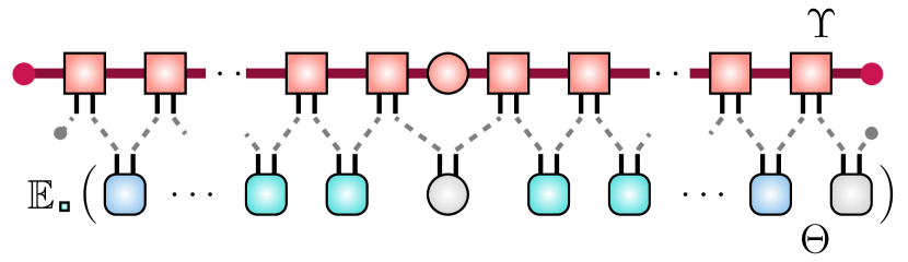
Figure 1: Randomized Benchmarking as a contraction of Matrix Product Operators. On top, the noise tensor $\Upsilon$, with unitary noise maps $\Lambda_{i}$ (red squares) and the fiducial state $\rho_{\mathsf{E}}$ (red circle), is correlated via an environment of bond dimension (red thick line) at most equal to $d_{\mathsf{E}}$, while below a control tensor $\Theta$ contains all the gates $\mathcal{G}_{i}$ (green/blue rounded squares), the initial state $\rho_{\mathsf{S}}$ (gray circle) and the measurement $M$ (gray rounded square). Averaging over gates, denoted $\mathds{E}$ is done over $\Theta$ (resulting effectively in a sum of MPO s). In dashed lines is denoted the contraction order, while bullets denote contractions at the edges.

We may generally describe non-Markovianity as mediated by an external environment: in the quantum case, this corresponds to a Hilbert space $\mathscr{H}_{\mathsf{E}}$ part of a total composite $\mathscr{H}_{\mathsf{E}}\otimes\mathscr{H}_{\mathsf{S}}$, with the labels $\mathsf{E}$ and $\mathsf{S}$ corresponding to environment and system of interest, respectively. A non-Markovian RB sequence may be described as follows. An initial state $\rho_{\mathsf{S}}$ is prepared on $\mathsf{S}$, which then can interact with $\mathsf{E}$, initially in some fiducial state $\rho_{\mathsf{E}}$, via a Completely Positive (CP) map $\Lambda_{0}$ acting jointly on $\mathsf{S}\mathsf{E}$, until a gate $\mathcal{G}_{1}$ is applied on system $\mathsf{S}$, followed by a CP map $\Lambda_{1}$, and so on, until the undo gate $\mathcal{G}_{m+1}=\mathcal{G}_{1}^{-1}\circ\cdots\circ\mathcal{G}_{m}^{-1}$ is applied followed by noise $\Lambda_{m+1}$ and a Positive Operator Valued Measurement (POVM) element $M$ solely on $\mathsf{S}$. Sequences such as this one, together with all statistics and $(m+1)$-point correlations, are described by the process tensor framework [24, 26, 27, 28, 29, 8, 30, 31, 32], whereby the inherent noise dynamics of the full $\mathsf{S}\mathsf{E}$ can be given in a tensor $\mathscr{Y}_{m+1}$, and the sequence of gates in a tensor $\mathscr{G}_{m+1}$.

The expectation of $M$, averaged over the quantum gates, is known as the Average Sequence Fidelity (ASF), and can now be computed as

$$\mathcal{F}_{m}=\operatorname{tr}\left\{M\operatorname{tr}_{\overline{\mathsf{S}}}\left[\mathscr{Y}_{m+1}\mathds{E}\left(\mathscr{G}_{m+1}^{\mathrm{T}}\right)\right]\right\},$$ (2)

where $\mathds{E}$ is an average over uniformly sampled gates $\mathcal{G}_{i}$, $\operatorname{tr}_{\overline{\mathsf{S}}}$ is partial trace over all auxiliary systems in the tensors, except $\mathsf{S}$, and the corresponding tensors can be defined through their Choi state representation  by

$$\mathscr{Y}_{m+1} :=\operatorname{tr}_{\mathsf{E}}\left[\operatorname*{\text{\raisebox{1.07639pt}{\scalebox{0.7}{$\bigcirc$}}}}_{i=1}^{m+1}\left(\Lambda_{i}\circ\mathscr{S}_{i}\right)\left(\rho\otimes\psi^{\otimes{m+1}}\right)\right]$$ (3)

$$\mathscr{G}_{m+1} =\mathds{1}_{\mathsf{S}}\otimes\operatorname*{\text{\raisebox{1.07639pt}{\scalebox{0.6}{$\bigotimes$}}}}_{i=1}^{m+1}\left(\mathds{1}_{\mathsf{A}_{i}}\otimes\mathcal{G}_{i}\right)\psi^{\otimes{m+1}},$$ (4)

where here $\circ$ is a composition of maps, $\rho:=\Lambda_{0}(\rho_{\mathsf{S}}\otimes\rho_{\mathsf{E}})$ and $\psi=\sum|ii\rangle\!\langle{jj}|$ are unnormalized maximally entangled states defined in auxiliary spaces $\mathsf{A}_{1}\mathsf{B}_{1}\cdots\mathsf{A}_{m+1}\mathsf{B}_{m+1}$; the map $\mathscr{S}_{i}$ is a swap between system $\mathsf{S}$ and the $i$^th ancillary space $\mathsf{A}_{i}$.

The ASF is the analytical form of the data estimated by the RB protocol. Whenever the underlying noise is approximated as Markovian, time-independent, gate-independent and trace-preserving, it can be seen that the ASF in Eq. (2) reduces to $\mathcal{F}_{m}=Ap^{m}+B$, where $p$ is directly related to the average gate fidelity of $\Lambda$ with respect to the identity, and $A$ and $B$ are constants only depending on SPAM errors.

The Choi state representation of the process tensor is simply a many-body state (up to normalization) translating its temporal correlations into spatial ones; naturally, as any other many-body operator, it admits a MPO decomposition [24, 8], i.e., it can be expressed as a chain of contractions of single operators. We can thus rearrange the noise process, i.e., all $\Lambda_{i}$ CP maps and the fiducial state $\rho_{\mathsf{E}}$, as a MPO $\Upsilon_{m+1}$, and the control process, i.e., the gates $\mathcal{G}_{i}$, the initial state $\rho_{\mathsf{S}}$, and the measurement element $M$, respectively, as another MPO, $\Theta_{m+1}$, such that

$$\mathcal{F}_{m} =\operatorname{tr}\left[\Upsilon_{m+1}\Theta_{m+1}^{\dagger}\right].$$ (5)

This is depicted graphically for the case of unitary noise in Fig. 1, where the free legs in each tensor represent the corresponding degrees of freedom in $\mathsf{S}$ and the thick line joining each node of $\Upsilon$ represents its so-called bond dimension. We derive both MPO s explicitly in Appendix B, with which the inner product in Eq. (5) can be written explicitly as a sum over their degrees of freedom in $\mathsf{S}$.

The MPO decomposition of the process tensor opens up new possibilities to efficiently study features of non-Markovian processes [34]. While the dimension of $\mathscr{Y}_{m+1}$ in Eq. (3) grows exponentially in sequence length, the construction of the MPO $\Upsilon_{m+1}$ can be made with a complexity scaling linearly in sequence length, and similarly for the control tensor $\Theta_{m+1}$. Furthermore, while generically the dimension $d_{\mathsf{E}}$ of the environment is large, the bond dimension of $\Upsilon_{m+1}$ will usually be much smaller, as often only a finite part of the environment interacts with the system at a given time [35, 34]. The bond dimension of $\Upsilon_{m+1}$ corresponds precisely to this minimal dimension, $d_{\mathsf{eff}}$, for an environment to propagate memory through different timesteps. In the context of RB, then, deviations from an exponential decay of the ASF can be directly tied to the bond dimension of the noise tensor.

We now show how these features can be extracted from a RB experiment’s data alone, thereby quantifying average non-Markovianity rates, by employing the machine learning techniques devised in [23].

II Supervised Learning for non-Markovian RB

The use of MPO s has already proven useful for the numerical and conceptual investigation of open quantum systems, e.g., in [36, 37, 38, 39, 34], and are still an active subject of investigation. Tensor networks, of which MPO s are particular cases, naturally find applications for machine learning tasks [23, 40, 41, 42, 43, 44, 45, 46], and can further serve to learn full process tensors [47]. Here we show a way to train a model that allows to learn the effective average non-Markovianity from a RB experiment’s data.

The outputs of a RB experiment are estimations of the ASF in Eq. (5). Let $\{\mathcal{F}^{(\mathrm{exp})}_{n}\}_{n=1}^{m}$ be such outputs, which are real numbers between 0 and 1 with a given uncertainty, for an experiment with a given gate set $\{\mathcal{G}_{i}\}_{i=1}^{m}$, target initial state $\rho_{\mathsf{S}}$ and measurement $M$. Thus we aim to be able to estimate a model for the underlying noise giving rise to such statistics: in particular we want to extract an effective environment dimension and an effective noise memory length. To do so, we must optimize a cost function relating the known outputs with our model; concretely, we choose to optimize the quadratic cost

$$C :=\frac{1}{2}\sum_{n=1}^{m}\left(\mathcal{F}_{n}-\mathcal{F}^{(\mathrm{exp})}_{n}\right)^{2},$$ (6)

by adapting the sweeping algorithm of [23] for the MPO representation of the process tensor as follows.

The sweeping algorithm is an iterative method that proceeds by updating pairs of nodes of the corresponding MPO model by gradient descent. We adapt this method to the process tensor by fixing an environment dimension and demanding physicality of the noise, i.e. that the nodes in the noise tensor $\Upsilon$ constitute at least CP maps. We choose to ensure this by assuming a closed $\mathsf{S}\mathsf{E}$ system, i.e., that all the nodes $\lambda_{i}$ in $\Upsilon$ are unitary . Demanding the learned MPO to be physical is the major difference between our method and the original sweeping algorithm.

Projected gradient descent is a method to solve a constraint optimization problem: it projects the gradient onto the constraint set. In our method, we project a square matrix $X$ onto an unitary constraint set, $Q_{U}$. This projection $\pi(X)$ is implemented by an optimization $\pi(X)=\arg\min_{Q\in Q_{U}}\|X-Q\|^{2}$. Practically, this projection has a simpler implementation as shown in [48]: the solution can be reached by taking Singular Value Decomposition (SVD) on the matrix $X$, resulting in two unitaries $U,V^{\dagger}$ and a singular matrix $S$. The solution is simply given by replacing the singular matrix by an identity one, $\pi(X)=UV^{\dagger}$.

Briefly summarized, our algorithm proceeds as follows (full detail can be seen in Appendix C):

1. Contract a neighboring pair of node tensors $\lambda_{i}$, $\lambda_{i+1}$ in $\Upsilon$ to form a single joint node, $L_{i,i+1}$.

2. Compute the gradient of the cost function with respect to the joint node, $\Delta{L}_{i,i+1}$, and update the joint node as $L^{\prime}_{i,i+1}=L_{i,i+1}+\alpha\Delta{L}_{i,i+1}$ with some learning rate $\alpha$. Methods such as Adagrad [49] or Adam [50] allow for an optimal choice of $\alpha$.

3. Split the updated joint node by a higher dimensional SVD [51] and decompose a tensor to be the multiplication of as $L^{\prime}_{i,i+1}=(A\sqrt{S})(\sqrt{S}B^{\dagger})$, where $(A\sqrt{S})$ and $(\sqrt{S}B^{\dagger})$ are both $d_{\mathsf{E}}d_{\mathsf{S}}^{2}$ square matrices. Keeping the columns corresponding to the largest $d_{\mathsf{E}}$ singular values, truncate the unitaries $A\sqrt{S}\to{\tilde{a}}$, $\sqrt{S}B\to{\tilde{b}}$ to $(d_{\mathsf{E}}d_{\mathsf{S}}^{2}\times d_{\mathsf{E}})$ matrices. And reshape the truncated matrices to square $d_{\mathsf{E}}d_{\mathsf{S}}$ matrices, $\tilde{a}\to{a}$, $\tilde{b}\to{b}$.

4. Project the truncated matrices to be unitary. We follow [48] by performing a further SVD as $a=U_{a}S_{a}V_{a}^{\dagger}$ and $b=U_{b}S_{b}V_{b}^{\dagger}$. The projections of $a$ and $b$ are $U_{a}V_{a}^{\dagger}$ and $U_{b}V_{b}^{\dagger}$, respectively. Multipy them to form a new node $\lambda\to{U}_{a}V_{a}^{\dagger}{V}_{b}{U}_{b}^{\dagger}$.

5. Update all the nodes in $\Upsilon$ as $\lambda\to{U}_{a}V_{a}^{\dagger}{V}_{b}{U}_{b}^{\dagger}$ and $\lambda^{\dagger}\to{U}_{b}V_{b}^{\dagger}{V}_{a}{U}_{a}^{\dagger}$. By updating all the nodes we thereby impose time-independence, which speeds up the update process and avoids over-fitting.

6. Return to point 1 with another pair of nodes, aiming to minimize the cost function $C$.

When the fitting model converges to the experimental data, according to a user-specified criterion, and the cost function in Eq. (6) is minimized, the structure of the resulting tensor will reflect whether the data is Markovian or not. This shall occur either within its bond-dimension, or equivalently in the form of the nodes themselves (e.g., whether they are correlated with the whole of $\mathsf{E}$ or not). The learned noise model itself will be irrelevant and should be simply thought of as an effective average model giving rise to the experimental RB data. Then, the very first step to test this is that employ this method to discriminate a non-Markovian noise model from a Markovian one. An effective, albeit artificial, model of the noise tensor, reflecting the average non-Markovianity of the data, or lack thereof, can then be learned for any choice of initial states, measurements and/or gate sets.

We now show two proof-of-principle examples that demonstrate our method.

III Numerical examples

In the following, we start by performing standard RB with Clifford gates on two different noise models and estimating the corresponding ASF over 100 samples. This will serve as our RB data, on which we aim our method to estimate the minimal environment size giving rise to it and some effective noise models which need not match the true noise other than precisely in the required environment size.

In both cases, for our learning model, we consider one qubit as our system $\mathsf{S}$ and one qubit as environment $\mathsf{E}$, initially on state $\rho=|00\rangle\!\langle 00|$ and a projective measurement $\mathcal{M}=|0\rangle\!\langle 0|$. The same procedure can be performed for distinct gate sets, as well as initial states and measurements to generalize the learning model.

We observed sudden jumps in the cost function in both cases. This might be a consequence of the time-independence constraint we imposed, suddenly updating it away from the minimum. A more detailed discussion on this issue is in Appendix E.3. Updating only a pair of nodes in a single iteration could provide a better fit at the expense of an increase in iterations of as many times as the sequence length of the experiment; we discuss this possibility in Sec. IV

III.1 Markovian phase flip noise model

We consider the single-qubit phase flip channel, $\mathcal{E}(\cdot)=\sum_{i=0}^{1}E_{i}(\cdot)E_{i}^{\dagger}$, where $E_{0}=\sqrt{1-p}\mathds{1}$ and $E_{1}=\sqrt{p}{Z}$, where $p$ is the phase flip probability, which we fix to $p=0.06$. The corresponding numerical ASF, the learned points and the cost function as a function of iterations is depicted in Fig. 2. The learned points converged in 19 iterations as the cost function approached a local minimum. The cost function can be seen to first approach such minimum, although afterwards it increases and displays at least one jump far from the minimum.

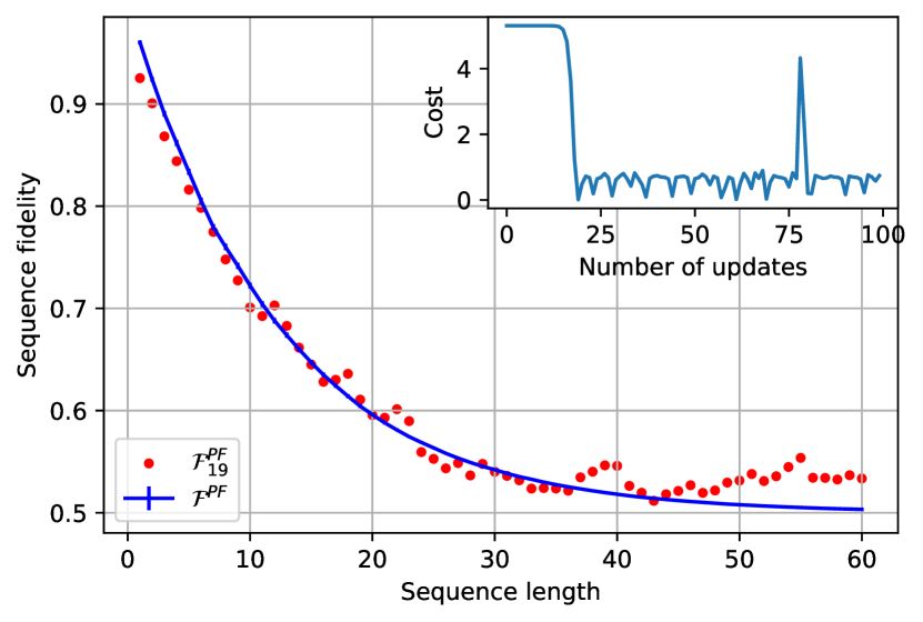
Figure 2: Learned ASF for Markovian phase flip noise. The blue line is the ASF from the noise model and the error bar is the standard deviation divided by square root of sample numbers (too small to be seen). The red dots are the output of our method, obtained by Adagrad [49] with initial learning rate $\alpha=10^{-5}$. The superscript in $\mathcal{F}^{PF}_{19}$ indicates the noise model and the subscript is the number of iterations to reach this result. The subplot shows the change of cost with iterations, the $19^{\textit{th}}$ iteration gives the ASF data shown in here.

Crucially, the learned unitary noise has the form of a direct sum, $\lambda=\mathds{1}_{\mathsf{E}}\oplus u$ where $u$ is a unitary solely on $\mathsf{S}$, implying uncorrelated noise. As shown in Appendix E.1 in another example with an amplitude damping noise model, this is a consistent feature of the method when the noise is Markovian. This reflects that no environment is needed, as there is no temporal correlations, or memory, between time-steps within the noise. This might then be generalized both to identify an ASF’s data as Markovian or non-Markovian, as well as to more generally infer the minimal size of the correlation needed with an environment to produce such data.

III.2 Two qubit non-Markovian spin noise model

We consider the two qubit fully non-Markovian spin noise model from [21], given that RB exponential deviations on it are manifest. It is a static unitary noise model $\Lambda(\cdot)=\lambda(\cdot)\lambda^{\dagger}$, where $\lambda=\exp(-i\delta H)$ for small positive $\delta$. The Hamiltonian is given by the two-spin interaction $H=JX_{1}X_{2}+h_{x}\left(X_{1}+X_{2}\right)+h_{y}\left(Y_{1}+Y_{2}\right)$, with $X_{i}$ and $Y_{i}$ being respective Pauli matrices acting on the $i$^th site. The ASF data, $\mathcal{F}^{nM}$ in Fig. 3, is generated by the model with $J=1.2,h_{x}=1.17,h_{y}=-1.15$ and $\delta=0.05$. The cost function updates away from the minimum after two jumps: we discuss this issue further in Appendix E.3.

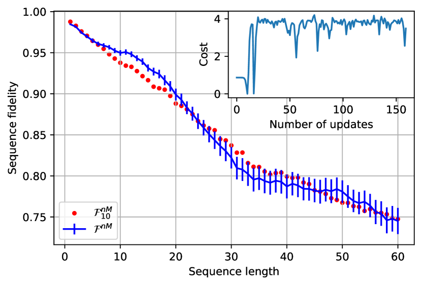
Figure 3: Learned ASF for two qubit fully non-Markovain spin noise model. The blue line is the ASF from the non-Markovian noise model and the error bar is the standard deviation divided by square root of sample numbers. The red dots are the output of our method, obtained by Adam [50] with learning rate $\alpha=0.001$ and Adam decay rates $\beta_{1}=0.9$, $\beta_{2}=0.99$. The superscript in $\mathcal{F}^{nM}_{10}$ indicates the noise model and the subscript is the number of iterations to reach this result. The subplot shows the change of cost with iterations, the $10^{\textit{th}}$ iteration gives the ASF data shown in here.

We expect that the learned noise has a form which indicates the interaction among $\mathsf{S}$ and $\mathsf{E}$. As shown in Appendix E.2, it can be seen that the environment qubit is always needed. While our method correctly keeps the environment qubit, it can be seen that the deviations from an exponential between the sequence lengths $10$ to $20$ in Fig. 3 are not completely resolved by the fit. This might again be related to the time-independence constraint, which we discuss further below.

IV Conclusions and Discussion

We propose a method to deduce the average non-Markovianity, as specified by the minimal environment size, within the underlying noise dynamics producing a given Randomized Benchmarking (RB) experiment’s data. We demonstrate numerically in two proof-of-principle examples that our method is able to distinguish between the RB data of a Markovian and a non-Markovian noise model. We furthermore argue how this method is more generally able to deduce the minimal effective environment dimension required to produce a given RB data, as this becomes manifest in the correlation structure of the learned effective noise.

While in this manuscript we present examples restricted to time-independent noise, our method is amenable to be extended for more complex cases such as a finite length non-Markovian noise. This presents new challenges, as the method might naively overfit the data by simply allowing distinct noise $\Lambda_{i}$ solely on system $\mathsf{S}$ such that a decay of the form $\mathcal{F}_{m}=Ap_{1}p_{2}\cdots{p}_{m}+B$ is obtained (unless the data is purely non-Markovian and displays a fidelity increase in sequence length [22]). Another challenge is that time-dependence would impose a substantial computing overhead, as we would need at least the same amount of iterations of the sweeping algorithm as the given sequence length to do a single update of all the nodes. The constraint to time-independence (described in detail in Appendix C), is imposed in the method by replacing all the noise nodes by the updated one on each iteration of the sweeping algorithm. Similarly, while we opt to enforce the learning method to be constrained to physical noise by demanding the full $\mathsf{S}\mathsf{E}$ to be a closed system, this can be relaxed to simply demanding that the noise is represented at least by a Completely Positive (CP) map on $\mathsf{S}\mathsf{E}$. While this may alleviate having to set a larger dimension of $\mathsf{E}$ in case the real minimal such dimension is larger, it also imposes an overhead in having to fit, in principle, all $d_{\mathsf{E}}^{2}d_{\mathsf{S}}^{2}$ Kraus operators.

A more fundamental way to improve the foreseen efficiency problem might be doing gradient descent on all the tensors at the same time. This can be achieved by the direct gradient descent (DGD) technique in [52]. They improve the exploding or vanishing gradients for tensor networks via an initialization scheme. Transforming our task to a DGD problem would be a worth exploring approach.

In this work, we show that it remains feasible to extract relevant information from the mere simplicity a RB experiment’s data, namely, about directly inaccessible temporal correlations within a device’s quantum noise. Our method can furthermore be extended and tailored for specific purpose routines; this is increasingly relevant as the development of quantum devices continues to scale up, with non-Markovianity remaining one of the major challenges largely unresolved.

V Acknowledgement

SXY thanks Ming-Chien Hsu and Shih-Min Yang for fruitful discussion. SXY and PFR thank Mathias Jørgensen for helpful comments and suggestions. The authors thank Dario Poletti and Guo Chu for insightful discussion.

Appendix A Randomized benchmarking for non-Markovian noise

A.1 The randomized benchmarking protocol

A standard Randomized Benchmarking (RB) experimental protocol proceeds as follows:

1. Prepare an initial state $\rho_{\mathsf{S}}$ on the system of interest $\mathsf{S}$.

2. Sample $m$ distinct elements, $\mathcal{G}_{1},\mathcal{G}_{2},\ldots,\mathcal{G}_{m}$, uniformly at random from a given gate set $\mathds{G}$. Let $\mathcal{G}_{m+1}:=\operatorname*{\text{\raisebox{1.07639pt}{\scalebox{0.7}{$\bigcirc$}}}}_{i=m}^{1}\mathcal{G}_{i}^{\dagger}=\mathcal{G}_{1}^{\dagger}\circ\cdots\circ\mathcal{G}_{m}^{\dagger}$, where $\circ$ denotes composition of maps, and $\mathcal{G}^{\dagger}(\cdot)=G^{\dagger}(\cdot)G$ for any Kraus representation with unitaries $G$ of the map $\mathcal{G}$. We refer to $\mathcal{G}_{m+1}$ as an undo-gate.

3. Apply the composition $\operatorname*{\text{\raisebox{1.07639pt}{\scalebox{0.7}{$\bigcirc$}}}}_{i=1}^{m+1}\mathcal{G}_{i}$ on $\rho_{\mathsf{S}}$. In practice, this amounts to applying a noisy sequence $\mathcal{S}_{m}:=\operatorname*{\text{\raisebox{1.07639pt}{\scalebox{0.7}{$\bigcirc$}}}}_{i=1}^{m+1}\tilde{\mathcal{G}}_{i}$ of length $m$ on $\rho_{\mathsf{S}}$, where $\tilde{\mathcal{G}}_{i}$ are the physical noisy gates associated to $\mathcal{G}$.

4. Estimate the probability $f_{m}:=\operatorname{tr}\left[M{\mathcal{S}}_{m}\left(\rho\right)\right]$ via a Positive Operator Valued Measurement (POVM) element $M$.

5. Repeat $n$ times the steps 1 to 4 for the same initial state $\rho_{\mathsf{S}}$, same POVM element $M$, and different sets of gates chosen uniformly at random $\{\mathcal{G}_{i}^{(1)}\}_{i=1}^{m},\{\mathcal{G}_{i}^{(2)}\}_{i=1}^{m},\ldots,\{\mathcal{G}_{i}^{(n)}\}_{i=1}^{m}$ from $\mathds{G}$ to obtain the probabilities $f_{m}^{(1)},f_{m}^{(2)},\ldots{f}_{m}^{(n)}$. Compute the Average Sequence Fidelity (ASF), $\mathcal{F}_{m}=1/n\sum_{i=1}^{n}f_{m}^{(i)}$.

6. Examine the behavior of the ASF, $\mathcal{F}_{m}$, over different sequence lengths $m$.

A.2 The process tensor and non-Markovianity

Appendix B The noise process tensor (model) and the control tensor (input)

We want to compute the ASF for a sequence of $m+1$ noisy gates with an initial state $\rho_{\mathsf{S}}$ and a POVM element ${M}$, written as a contraction of tensors

$$\mathcal{F}_{m} =\mathds{E}\left[\Upsilon_{m+1}\ast\Theta_{m+1}(\rho_{\mathsf{S}},{M})\right]$$ (7)

$$=\mathds{E}\big{\{}\sum_{\vec{s}_{m+1}^{\,\,(\prime)},\,\vec{\zeta}_{m+1}^{\,\,(\prime)}}\Upsilon_{\vec{s}_{m+1}^{\,\,(\prime)}\vec{\zeta}_{m+1}^{\,\,(\prime)}}\,\Theta_{\vec{s}_{m+1}^{\,\,(\prime)}\vec{\zeta}_{m+1}^{\,\,(\prime)}}\big{\}}.$$ (8)

where $\mathds{E}$ is average over gates, and $\ast$ here means an interior product

$$A\ast{B}=\operatorname{tr}[AB^{\dagger}],$$ (9)

of the tensors $A$ and $B$, and $\vec{s}_{i}^{\,\,(\prime)}=(s_{0},s_{0}^{\prime},s_{1},s_{1}^{\prime},\ldots,s_{i},s_{i}^{\prime})$, and similarly for $\vec{\zeta}^{\,\,(\prime)}_{i}$. Crucially, only the tensor $\Upsilon$ contains information about the noise and the environment $\mathsf{E}$.

We can identify the Matrix Product Operator (MPO) form of the tensors $\Upsilon$ and $\Theta$ by writing

$$\mathcal{F}_{m}=\operatorname{tr}\{\mathscr{Y}_{m+1}\,\mathds{E}(\mathscr{G}_{m+1}^{\mathrm{T}})\},$$ (10)

where $\mathscr{Y}$ is the Choi state of the noise process and $\mathscr{G}$ is the Choi state of the gate sequence, which is subsequently averaged ($\mathds{E}$) over gates; explicitly, these are defined by

$$\mathscr{Y}_{m+1}:=\operatorname{tr}_{\mathsf{E}}\left[\Lambda_{m+1}\circ\mathscr{S}_{m+1}\circ\cdots\circ\Lambda_{1}\circ\mathscr{S}_{1}\circ\Lambda_{0}\left(\rho_{\mathsf{E}}\otimes\rho_{\mathsf{S}}\otimes\psi^{\otimes{m+1}}\right)\right],$$ (11)

where $\Lambda_{i}$ is the gate independent and Completely Positive (CP) noise map at step $i$ acting on $\mathsf{S}\mathsf{E}$, $\psi=\sum_{i,j=1}^{d_{\mathsf{S}}}|ii\rangle\!\langle{jj}|$ is an unnormalized maximally entangled state, with each copy defined on auxiliary spaces $\mathsf{A}_{1}\mathsf{B}_{1},\ldots,\mathsf{A}_{m+1}\mathsf{B}_{m+1}$, $\mathscr{S}_{i}$ is a swap operator between $\mathsf{S}$ and half of the $i$^th auxiliary space, say $\mathsf{A}_{i}$, and $\rho_{\mathsf{E}}$ is a fiducial state of $\mathsf{E}$; on the other hand,

$$\mathscr{G}_{m+1} ={M}^{\mathrm{T}}\otimes\left(\mathds{1}_{\mathsf{A}_{1}}\otimes\mathcal{G}_{1}\otimes\mathds{1}_{\mathsf{A}_{2}}\otimes\mathcal{G}_{2}\otimes\cdots\otimes\mathds{1}_{\mathsf{A}_{m+1}}\otimes\mathcal{G}_{m+1}\right)\psi^{\otimes{m+1}},$$ (12)

with $\mathcal{G}_{i}$ the applied gate at step $i$. This definition is different from that in the main text in Eq. (4) simply in that here we incorporate directly the measurement $M$. Notice that the gates $\mathcal{G}_{i}$ have to be defined on the complementary auxiliary spaces, $\mathsf{B}_{i}$, because the swaps in Eq. (11) were defined with resp to $\mathsf{A}_{i}$. Finally, keep in mind that $\mathcal{G}_{m+1}$ is the undo (sequence of inverses) gate.

The only difference between $\mathscr{Y}$ and $\Upsilon$, and between $\mathds{E}[\mathscr{G}^{\mathrm{T}}]$ and $\Theta$ is the dependence of $\rho_{\mathsf{S}}$: we want all the inputs in a MPO separate from one containing solely the noise. For this reason, henceforth we refer to $\Upsilon$ as the noise tensor (or MPO) and to $\Theta$ as the control tensor (or MPO).

Consider $m=1$. Denote $\rho:=\Lambda_{0}(\rho_{\mathsf{E}}\otimes\rho_{\mathsf{S}})$ and let $\mathfrak{S}_{\alpha\beta}:=\mathds{1}_{\mathsf{E}}\otimes|\alpha\rangle\!\langle\beta|$, then

$$\mathscr{Y}_{2}:=\operatorname{tr}_{\mathsf{E}}[\Lambda_{2}\circ\mathscr{S}_{2}\circ\Lambda_{1}\circ\mathscr{S}_{1}\circ(\rho\otimes\psi^{\otimes 2})]$$

$$=\sum\operatorname{tr}_{\mathsf{E}}[\lambda_{2}^{\mu}\mathfrak{S}_{\alpha_{2}\beta_{2}}\lambda_{1}^{\nu}\mathfrak{S}_{\alpha_{1}\beta_{1}}\rho\mathfrak{S}_{\delta_{1}\gamma_{1}}\lambda_{1}^{\dagger\,\nu}\mathfrak{S}_{\delta_{2}\gamma_{2}}\lambda_{2}^{\dagger\,\mu}]\otimes|\beta_{1}\rangle\!\langle\alpha_{1}|i_{1}\rangle\!\langle{j_{1}}|\gamma_{1}\rangle\!\langle\delta_{1}|\otimes|i_{1}\rangle\!\langle{j}_{1}|\otimes|\beta_{2}\rangle\!\langle\alpha_{2}|i_{2}\rangle\!\langle{j_{2}}|\gamma_{2}\rangle\!\langle\delta_{2}|\otimes|i_{2}\rangle\!\langle{j}_{2}|$$

$$=\sum\operatorname{tr}_{\mathsf{E}}[\lambda_{2}^{\mu}\mathfrak{S}_{\alpha_{2}\beta_{2}}\lambda_{1}^{\nu}\mathfrak{S}_{\alpha_{1}\beta_{1}}\rho\mathfrak{S}_{\delta_{1}\gamma_{1}}\lambda_{1}^{\dagger\,\nu}\mathfrak{S}_{\delta_{2}\gamma_{2}}\lambda_{2}^{\dagger\,\mu}]\otimes|\beta_{1}\alpha_{1}\beta_{2}\alpha_{2}\rangle\!\langle\delta_{1}\gamma_{1}\delta_{2}\gamma_{2}|,$$

$$=\sum(\langle{e}|\otimes\mathds{1}_{\mathsf{S}})\lambda_{2}^{\mu}|e_{2}\alpha_{2}\rangle\!\langle{e}_{2}\beta_{2}|\lambda_{1}^{\nu}|e_{1}\alpha_{1}\rangle\!\langle{e}_{1}\beta_{1}|\rho|\epsilon_{1}\delta_{1}\rangle\!\langle\epsilon_{1}\gamma_{1}|\lambda_{1}^{\dagger\,\nu}|\epsilon_{2}\delta_{2}\rangle\!\langle\epsilon_{2}\gamma_{2}|\lambda_{2}^{\dagger\,\mu}(|e\rangle\otimes\mathds{1}_{\mathsf{S}})\otimes|\beta_{1}\alpha_{1}\beta_{2}\alpha_{2}\rangle\!\langle\delta_{1}\gamma_{1}\delta_{2}\gamma_{2}|$$ (13)

where in the last line we inserted complete $\mathsf{E}$ orthonormal bases, and $\lambda_{i}^{\mu}$ are Kraus operators of $\Lambda_{i}$. Onward, we will denote components $\mathsf{S}\mathsf{E}$ of any $X$ matrix by

$$X_{ss^{\prime}}^{ee^{\prime}}:=\langle{e}s|X|e^{\prime}{s}^{\prime}\rangle.$$ (14)

Meanwhile,

$$\mathscr{G}_{2} ={M}^{\mathrm{T}}\otimes\left(\mathds{1}_{\mathsf{A}_{1}}\otimes\mathcal{G}\otimes\mathds{1}_{\mathsf{A}_{2}}\otimes\mathcal{G}^{\dagger}\right)\psi^{\otimes{2}}$$

$$=M^{\mathrm{T}}\otimes\sum|i_{1}\rangle\!\langle{j}_{1}|\otimes\mathcal{G}(|i_{1}\rangle\!\langle{j}_{1}|)\otimes|i_{2}\rangle\!\langle{j}_{2}|\otimes\tilde{\mathcal{G}}(|i_{2}\rangle\!\langle{j}_{2}|),$$ (15)

where here $\tilde{\mathcal{G}}:=\mathcal{G}^{-1}$ is the undo-gate, and thus

$$\operatorname{tr}[\mathscr{Y}_{2}\mathscr{G}_{2}^{\mathrm{T}}]=\sum(\lambda_{2}^{\mu})_{s\alpha_{2}}^{ee_{2}}(\lambda_{1}^{\nu})_{\beta_{2}\alpha_{1}}^{e_{2}e_{1}}\rho_{\beta_{1}\delta_{1}}^{e_{1}\epsilon_{1}}(\lambda_{1}^{\dagger\,\nu})^{\epsilon_{1}\epsilon_{2}}_{\gamma_{1}\delta_{2}}(\lambda_{2}^{\dagger\,\mu})^{\epsilon_{2}e}_{\gamma_{2}s^{\prime}}\langle{s}^{\prime}|{M}|s\rangle$$

$$\hskip 100.00015pt\langle\delta_{1}\gamma_{1}\delta_{2}\gamma_{2}|\left\{|j_{1}\rangle\!\langle{i}_{1}|\otimes\mathcal{G}(|i_{1}\rangle\!\langle{j}_{1}|)^{\mathrm{T}}\otimes|j_{2}\rangle\!\langle{i_{2}}|\otimes\tilde{\mathcal{G}}(|i_{2}\rangle\!\langle{j}_{2}|)^{\mathrm{T}}\right\}|\beta_{1}\alpha_{1}\beta_{2}\alpha_{2}\rangle$$

$$:=\sum(\lambda_{2}^{\mu})_{s\alpha_{2}}^{ee_{2}}(\lambda_{1}^{\nu})_{\beta_{2}\alpha_{1}}^{e_{2}e_{1}}\rho_{\beta_{1}\delta_{1}}^{e_{1}\epsilon_{1}}(\lambda_{1}^{\dagger\,\nu})^{\epsilon_{1}\epsilon_{2}}_{\gamma_{1}\delta_{2}}(\lambda_{2}^{\dagger\,\mu})^{\epsilon_{2}e}_{\gamma_{2}s^{\prime}}{M}_{s^{\prime}{s}}\,\langle\alpha_{1}|\mathcal{G}(|\beta_{1}\rangle\!\langle\delta_{1}|)|\gamma_{1}\rangle\!\langle\alpha_{2}|\tilde{\mathcal{G}}(|\beta_{2}\rangle\!\langle\delta_{2}|)|\gamma_{2}\rangle,$$ (16)

Let us now replace $\rho=\Lambda_{0}(\rho_{\mathsf{E}}\otimes\rho_{\mathsf{S}})$, and let $G$ be a unitary such that $\mathcal{G}(\cdot):=G(\cdot)G^{\dagger}$ and similarly, in order to track the undo-gate, let $\tilde{G}$ such that $\tilde{\mathcal{G}}:=\tilde{G}(\cdot)\tilde{G}^{\dagger}$; also let us relabel $\mathsf{S}$ indices to a more consistent notation with labels $s$ and $\zeta$ (with all contractions remaining the same), so that

$$\operatorname{tr}[\mathscr{Y}_{2}\mathscr{G}_{2}^{\mathrm{T}}]=\sum(\lambda_{2}^{\mu})_{s_{2}s_{2}^{\prime}}^{ee_{2}}(\lambda_{1}^{\nu})_{s_{1}s_{1}^{\prime}}^{e_{2}e_{1}}\rho_{s_{0}\zeta_{0}^{\prime}}^{e_{1}\epsilon_{1}}(\lambda_{1}^{\dagger\,\nu})_{\zeta_{1}\zeta_{1}^{\prime}}^{\epsilon_{1}\epsilon_{2}}(\lambda_{2}^{\dagger\,\mu})_{\zeta_{2}\zeta_{2}^{\prime}}^{\epsilon_{2}e}{M}_{\zeta_{2}^{\prime}s_{2}}\,\langle{s}_{1}^{\prime}|\mathcal{G}(|s_{0}\rangle\!\langle\zeta_{0}^{\prime}|)|\zeta_{1}\rangle\!\langle{s_{2}^{\prime}}|\tilde{\mathcal{G}}(|s_{1}\rangle\!\langle\zeta_{1}^{\prime}|)|\zeta_{2}\rangle$$

$$=\sum(\lambda_{2}^{\mu})_{s_{2}s_{2}^{\prime}}^{ee_{2}}(\lambda_{1}^{\nu})_{s_{1}s_{1}^{\prime}}^{e_{2}e_{1}}(\lambda_{0}^{\sigma})_{s_{0}s_{0}^{\prime}}^{e_{1}e_{0}}(\rho_{\mathsf{E}})^{e_{0}\epsilon_{0}}(\rho_{\mathsf{S}})_{s_{0}^{\prime}\zeta_{0}}(\lambda_{0}^{\dagger\,\sigma})_{\zeta_{0}\zeta_{0}^{\prime}}^{\epsilon_{0}\epsilon_{1}}(\lambda_{1}^{\dagger\,\nu})_{\zeta_{1}\zeta_{1}^{\prime}}^{\epsilon_{1}\epsilon_{2}}(\lambda_{2}^{\dagger\,\mu})_{\zeta_{2}\zeta_{2}^{\prime}}^{\epsilon_{2}e}{M}_{\zeta_{2}^{\prime}s_{2}}G_{{s}_{1}^{\prime}s_{0}}G^{\dagger}_{\zeta_{0}^{\prime}\zeta_{1}}\tilde{G}_{s_{2}^{\prime}s_{1}}\tilde{G}^{\dagger}_{\zeta_{1}^{\prime}\zeta_{2}},$$ (17)

so we may now identify

$$\Upsilon_{\vec{s}_{2}^{\,\,(\prime)}\vec{\zeta}_{2}^{\,\,(\prime)}} =\sum_{\mu,\nu,\sigma}\sum_{e_{i},\epsilon_{i}}(\lambda_{2}^{\mu})_{s_{2}s_{2}^{\prime}}^{ee_{2}}(\lambda_{1}^{\nu})_{s_{1}s_{1}^{\prime}}^{e_{2}e_{1}}(\lambda_{0}^{\sigma})_{s_{0}s_{0}^{\prime}}^{e_{1}e_{0}}(\rho_{\mathsf{E}})^{e_{0}\epsilon_{0}}(\lambda_{0}^{\dagger\,\sigma})_{\zeta_{0}\zeta_{0}^{\prime}}^{\epsilon_{0}\epsilon_{1}}(\lambda_{1}^{\dagger\,\nu})_{\zeta_{1}\zeta_{1}^{\prime}}^{\epsilon_{1}\epsilon_{2}}(\lambda_{2}^{\dagger\,\mu})_{\zeta_{2}\zeta_{2}^{\prime}}^{\epsilon_{2}e},$$ (18)

$$\Theta_{\vec{s}_{2}^{\,\,(\prime)}\vec{\zeta}_{2}^{\,\,(\prime)}} =\tilde{G}_{s_{2}^{\prime}{s}_{1}}\,G_{s_{1}^{\prime}{s}_{0}}\,(\rho_{\mathsf{S}})_{s_{0}^{\prime}\zeta_{0}}\,G^{\dagger}_{\zeta_{0}^{\prime}\zeta_{1}}\,\tilde{G}^{\dagger}_{\zeta_{1}^{\prime}\zeta_{2}}\,{M}_{\zeta_{2}^{\prime}s_{2}},$$ (19)

so generally for any $m\geq 1$,

$$\Upsilon_{\vec{s}_{m+1}^{\,\,(\prime)}\vec{\zeta}_{m+1}^{\,\,(\prime)}} =\sum_{\mu_{i}}\sum_{\{e,\epsilon\}}(\lambda_{m+1}^{\mu_{m+1}})_{s_{m+1}s_{m+1}^{\prime}}^{ee_{m+1}}\left[\prod_{i=0}^{m}(\lambda_{i}^{\mu_{i}})_{s_{i}s_{i}^{\prime}}^{e_{i+1}e_{i}}\right](\rho_{\mathsf{E}})^{e_{0}\epsilon_{0}}\left[\prod_{j=0}^{m}(\lambda_{j}^{\dagger\,\mu_{j}})_{\zeta_{j}\zeta_{j}^{\prime}}^{\epsilon_{j}\epsilon_{j+1}}\right](\lambda_{m+1}^{\dagger\,\mu_{m+1}})_{\zeta_{m+1}\zeta_{m+1}^{\prime}}^{\epsilon_{m+1}e},$$ (20)

$$\Theta_{\vec{s}_{m+1}^{\,\,(\prime)}\vec{\zeta}_{m+1}^{\,\,(\prime)}} =\tilde{G}_{s_{m+1}^{\prime}s_{m}}\left[\prod_{i=1}^{m}(G_{i})_{s_{i}^{\prime}s_{i-1}}\right](\rho_{\mathsf{S}})_{s_{0}^{\prime}\zeta_{0}}\left[\prod_{j=1}^{m}(G^{\dagger}_{j})_{\zeta_{j-1}^{\prime}\zeta_{j}}\right]\tilde{G}^{\dagger}_{\zeta_{m}^{\prime}\zeta_{m+1}}\,{M}_{\zeta_{m+1}^{\prime}s_{m+1}},$$ (21)

where here $\mathcal{G}_{i}:=G_{i}(\cdot)G_{i}^{\dagger}$ is the gate at the $i$^th step for corresponding unitaries $G_{i}$, and $\tilde{G}:=\left(G_{m}G_{m-1}\cdots{G}_{1}\right)^{\dagger}$ gives the undo-gate $\tilde{\mathcal{G}}=\tilde{G}(\cdot)\tilde{G}^{\dagger}$. These tensors are depicted in Fig. 1 in the main text. Both tensors are of rank $4(m+2)$, i.e., each has $4(m+2)$ legs of dimension $d_{\mathsf{S}}$, and so there is a total of $d_{\mathsf{S}}^{\,4(m+2)}$ components to be specified on each.

Notice that if the $\Lambda_{i}$ matrices are unitary (so that all $\lambda_{i}^{\mu_{i}}$ have only a single $\mu_{i}$), then for $\Upsilon$ we require a memory scaling as $d_{\mathsf{E}}^{2}\left[1+(m+2)d_{\mathsf{S}}^{2}\right]$. Similarly, for $\Theta$ we require $\left(m+2\right)d_{\mathsf{S}}^{2}$ parameters. That is, we specify the nodes $\Lambda_{i}$, $\rho_{\mathsf{E}}$, $\mathcal{G}_{i}$, $\rho_{\mathsf{S}}$ and $M$ in each tensor to obtain either $\Upsilon$ or $\Theta$. Furthermore, assuming the size of the environment is sufficiently large, the effective bond dimension in $\Upsilon$ between timesteps need not necessarily be $d_{\mathsf{E}}$ but often will be smaller, giving rise to the effective noise dynamics specified by corresponding effective CP maps. Finally, notice that we may get rid of the complex conjugate in the final expressions and simply compute conjugates of entries. We thus would have, for unitary noise,

$$\Upsilon_{\vec{s}_{m+1}^{\,\,(\prime)}\vec{\zeta}_{m+1}^{\,\,(\prime)}} =\sum_{\{e,\epsilon\}}(\lambda_{m+1})_{s_{m+1}s_{m+1}^{\prime}}^{ee_{m+1}}\left[\prod_{i=0}^{m}(\lambda_{i})_{s_{i}s_{i}^{\prime}}^{e_{i+1}e_{i}}\right](\rho_{\mathsf{E}})^{e_{0}\epsilon_{0}}\left[\prod_{j=0}^{m}(\lambda_{j})_{\zeta_{j}^{\prime}\zeta_{j}}^{*\,\epsilon_{j+1}\epsilon_{j}}\right](\lambda_{m+1})_{\zeta_{m+1}^{\prime}\zeta_{m+1}}^{*e\epsilon_{m+1}},$$ (22)

$$\Theta_{\vec{s}_{m+1}^{\,\,(\prime)}\vec{\zeta}_{m+1}^{\,\,(\prime)}} =\mathds{E}\left\{\hat{G}^{*}_{s_{m}s_{m+1}^{\prime}}\left[\prod_{i=1}^{m}(G_{i})_{s_{i}^{\prime}s_{i-1}}\right](\rho_{\mathsf{S}})_{s_{0}^{\prime}\zeta_{0}}\left[\prod_{j=1}^{m}(G_{j})^{*}_{\zeta_{j}\zeta_{j-1}^{\prime}}\right]\hat{G}_{\zeta_{m}^{\prime}\zeta_{m+1}}\,{M}_{\zeta_{m+1}^{\prime}s_{m+1}}\right\},$$ (23)

where here $*$ denotes complex conjugate, and $\hat{G}:=G_{m}G_{m-1}\cdots{G}_{1}$.

A particular tensor that we will care about, is that obtained by a partial contraction of $\Upsilon_{m}$ and $\Theta_{m}$ whereby given nodes are not contracted. That is, denoting by $\Upsilon_{m}^{\{i,j,\ldots,k\}}$ a noise tensor without the $\lambda_{i}^{\mu_{i}}$, $\lambda_{j}^{\mu_{j}}$, …, $\lambda_{k}^{\mu_{k}}$ nodes (i.e., with such $\lambda$ terms not appearing in Eq. (20)), we define

$$\tilde{\Theta}_{m+1}^{\{i,j,\ldots,k\}}:=\sum\Upsilon^{\{i,j,\ldots,k\}}_{\vec{s}_{m+1}^{\,(\prime)}\vec{\zeta}_{m+1}^{\,(\prime)}}\Theta_{\vec{s}_{m+1}^{\,(\prime)}\vec{\zeta}_{m+1}^{\,(\prime)}},$$ (24)

as the contraction of all the tensors in the ASF of sequence length $m$, except for $\lambda_{i}$, $\lambda_{j}$, …, $\lambda_{k}$.

B.1 The (multi-qubit) Clifford group case

In [21], the average $\mathds{E}[\mathscr{G}^{\dagger}]=\mathds{E}[\mathscr{G}^{\mathrm{T}}]$ was analytically evaluated when the gates belong to the (multi-qubit) Clifford group, or more generally to any unitary 2-design, and the contraction with $\mathscr{Y}$ was done explicitly to obtain the ASF in Eq. (8), which can be written as

$$\mathcal{F}_{m} :=\operatorname{tr}\left[M\,\operatorname{tr}_{\mathsf{E}}\circ\Lambda_{m+1}\circ\left(\mathscr{A}_{m}+\mathscr{B}_{m}\right)\rho\right],$$ (25)

where

$$\mathscr{A}_{m}(\rho) :=\frac{\displaystyle{\operatorname*{\text{\raisebox{1.07639pt}{\scalebox{0.7}{$\bigcirc$}}}}_{n=1}^{m}}\left(\$_{\Lambda_{n}}-\pounds_{\Lambda_{n}}\right)\otimes\mathcal{I}_{\mathsf{S}}}{\left(d_{\mathsf{S}}^{2}-1\right)^{m}}\left(\rho-\tilde{\rho}_{\mathsf{E}}\otimes\frac{\mathds{1}}{d_{\mathsf{S}}}\right),$$ (26)

$$\mathscr{B}_{m}(\rho) :=\left(\operatorname*{\text{\raisebox{1.07639pt}{\scalebox{0.7}{$\bigcirc$}}}}_{n=1}^{m}\pounds_{\Lambda_{n}}\right)\tilde{\rho}_{\mathsf{E}}\otimes\frac{\mathds{1}}{d_{\mathsf{S}}},$$ (27)

with $\rho=\Lambda_{0}(\rho_{\mathsf{E}}\otimes\rho_{\mathsf{S}})$ and with $\tilde{\rho}_{\mathsf{E}}:=\operatorname{tr}_{\mathsf{S}}[\Lambda_{0}(\rho_{\mathsf{E}}\otimes\rho_{\mathsf{S}})]$; here $\$_{\Lambda_{n}},\pounds_{\Lambda_{n}}$ are maps acting solely on $\mathsf{E}$ as defined by

$$\$_{\Lambda_{n}}(\varepsilon) :=\sum_{s,s^{\prime}=1}^{d_{\mathsf{S}}}\langle{s}|\Lambda_{n}(\varepsilon\otimes|s\rangle\!\langle{s^{\prime}}|)|s^{\prime}\rangle$$ (28)

$$\pounds_{\Lambda_{n}}(\varepsilon) :=\operatorname{tr}_{\mathsf{S}}\left[\Lambda_{n}\left(\varepsilon\otimes\frac{\mathds{1}}{d_{\mathsf{S}}}\right)\right],$$ (29)

for any given operator $\varepsilon$ acting on $\mathsf{E}$. This is seen to imply that the tensor $\Theta_{m+1}$ is similar to the elements of a depolarizing tensor on $\mathsf{S}$, with components

$$\Theta_{\vec{s}_{m+1}^{\,(\prime)}\vec{\zeta}_{m+1}^{\,(\prime)}}=\left[\alpha_{\vec{s}_{m+1}^{\,(\prime)}\vec{\zeta}_{m+1}^{\,(\prime)}}+\beta_{\vec{s}_{m+1}^{\,(\prime)}\vec{\zeta}_{m+1}^{\,(\prime)}}\right](\rho_{\mathsf{S}})_{s_{0}^{\prime}\zeta_{0}}M_{\zeta^{\prime}_{m+1}s_{m+1}},$$ (30)

where here

$$\alpha_{\vec{s}_{m+1}^{\,(\prime)}\vec{\zeta}_{m+1}^{\,(\prime)}} :=\frac{\displaystyle{\prod_{n=1}^{m}}\left(d_{\mathsf{S}}\delta_{s_{n}s^{\prime}_{n}}\delta_{\zeta^{\prime}_{n}\zeta_{n}}-\delta_{s_{n}\zeta^{\prime}_{n}}\delta_{s^{\prime}_{n}\zeta_{n}}\right)}{d_{\mathsf{S}}^{m}(d_{\mathsf{S}}^{2}-1)^{m}}\left(\delta_{s_{0}s_{m+1}^{\prime}}\delta_{\zeta_{0}^{\prime}\zeta_{m+1}}-\frac{\delta_{s_{0}\zeta_{0}^{\prime}}\delta_{s^{\prime}_{m+1}\zeta_{m+1}}}{d_{\mathsf{S}}}\right)$$ (31)

$$\beta_{\vec{s}_{m+1}^{\,(\prime)}\vec{\zeta}_{m+1}^{\,(\prime)}} :=\frac{\displaystyle{\prod_{n=1}^{m}}\delta_{s_{n}\zeta^{\prime}_{n}}\delta_{s_{n}^{\prime}\zeta_{n}}}{d_{\mathsf{S}}^{m}}\left(\frac{\delta_{s_{0}\zeta_{0}^{\prime}}\delta_{s^{\prime}_{m+1}\zeta_{m+1}}}{d_{\mathsf{S}}}\right)$$ (32)

are the terms analogous to the $p$ and $1-p$ terms in the depolarizing channel. Notice that these definitions are slightly different to those made in [21]; this is simply because of the definition $\rho=\Lambda_{0}(\rho_{\mathsf{E}}\otimes\rho_{\mathsf{S}})$ and because $\Theta_{m}$ takes $\rho_{\mathsf{S}}$ while $\Upsilon_{m}$ takes $\lambda_{0}^{(\dagger)}$ and $\rho_{\mathsf{E}}$.

Appendix C Sweeping algorithm for Randomized Benchmarking

The so-called sweeping algorithm from [23] combines the idea of the kernel trick in [53] and the density matrix renormalization group (DMRG) algorithm in [54]: it is a tensor network supervised learning model which predicts outputs via the contraction of parameter tensor and input tensor. In a RB experiment, we obtain an experimental ASF and we choose the control tensor, but the underlying noise tensor generally remains unknown. Here we adapt the sweeping algorithm to obtain information about the average noise involved within a RB experiment. Taking the control tensor as an input tensor, the noise tensor as parameter tensor, and the experimental ASF as the label, we optimize the model until the predicted ASF is close enough (in a sense to be made precise below) to the experimental ASF.

More specifically, let us consider the noise tensor $\Upsilon_{m}$ written as the MPO in Eq. (20), for any fixed $m\geq 1$. Our goal is now to implement an extension of the sweeping algorithm above to learn features about $\Upsilon_{m}$, namely some model of the $\Lambda$ noise maps. While the corresponding RB experiment may be carried out with an arbitrary gate set, the closed expression in [21] for the Clifford group, can make the evaluation of the corresponding learned ASF, $\mathcal{F}_{m}$, in exact form readily available.

As opposed to the general sweeping algorithm, the noise tensor $\Upsilon_{m}$ has physical meaning, and thus it has certain constraints to follow. In particular, we fix all $\Lambda$ maps to be unitary. Imposing this unitarity constraint will allow us to sweep over only half the nodes of the noise tensor, thereby obtaining the rest by taking the adjoint of the updated nodes.

Let us then begin by defining a cost function

$$C :=\frac{1}{2}\sum_{n=1}^{m}\left(\mathcal{F}_{n}-\mathcal{F}^{(\mathrm{exp})}_{n}\right)^{2},$$ (33)

where as mentioned above, $\mathcal{F}^{(\mathrm{exp})}_{1}$, $\mathcal{F}^{(\mathrm{exp})}_{2}$, …, $\mathcal{F}^{(\mathrm{exp})}_{m}$, denote experimental ASF points for a RB sequence with up to length $m$, and $\mathcal{F}_{1}$, $\mathcal{F}_{2}$, …, $\mathcal{F}_{m}$ denote the learned points by the algorithm. The goal is then for the algorithm to determine noise maps $\Lambda$ that minimize $C$.

We now denote by $N_{\mathsf{E}}$ and $N_{\mathsf{S}}$ the number of qubits on the environment and system, respectively, so that $d_{\mathsf{E}}:=2^{N_{\mathsf{E}}}$ and $d_{\mathsf{S}}:=2^{N_{\mathsf{S}}}$. The algorithm will now proceed as described below. For fear that the fluency of the description will be break by the detail of constrained optimization, regarding Step 6, we will discuss it in Appendix D.

1. Set an appropriate $N_{\mathsf{E}}$, as discussed in the main text, and require all $\Lambda$ maps to be unitary, i.e., $\Lambda_{i}(\cdot):=\lambda_{i}(\cdot)\lambda_{i}^{\dagger}$ such that $\lambda_{i}\lambda_{i}^{\dagger}=\lambda_{i}^{\dagger}\lambda_{i}=\mathds{1}_{\mathsf{E}\mathsf{S}}$. Initialize each node $\lambda_{i}$ in the noise MPO $\Upsilon_{m}$; this choice is arbitrary, but here we employ identity matrices (i.e., we start assuming an absence of noise). Finally, set the initial state of the environment $\rho_{\mathsf{E}}=|0\rangle\!\langle 0|$; this choice is also arbitrary and fixed throughout the algorithm: any information about how this fiducial state changes is to be contained in the state preparation noise $\Lambda_{0}$.

2. Take any two neighboring nodes of the noise MPO, $\lambda_{i}$ and $\lambda_{i-1}$ for any $1\leq{i}\leq{m+1}$, and contract them on $\mathsf{E}$ into a joint node $L_{i,i-1}$, i.e.,

   $$(L_{i,i-1})^{e_{i+1}e_{i-1}}_{s_{i}s_{i}^{\prime}s_{i-1}s_{i-1}^{\prime}}:=\sum_{e_{i}}(\lambda_{i})_{s_{i}s_{i}^{\prime}}^{e_{i+1}e_{i}}(\lambda_{i-1})_{s_{i-1}s_{i-1}^{\prime}}^{e_{i}e_{i-1}},$$ (34)

   such that

   $$\Upsilon_{\vec{s}_{m+1}^{\,\,(\prime)}\vec{\zeta}_{m+1}^{\,\,(\prime)}} =\sum_{\{e,\epsilon\}/e_{i}}\cdots\left[\sum_{e_{i}}(\lambda_{i})_{s_{i}s_{i}^{\prime}}^{e_{i+1}e_{i}}(\lambda_{i-1})_{s_{i-1}s_{i-1}^{\prime}}^{e_{i}e_{i-1}}\right]\cdots(\lambda_{0})_{s_{0}s_{0}^{\prime}}^{e_{1}e_{0}}(\rho_{\mathsf{E}})^{e_{0}\epsilon_{0}}\cdots$$

   $$=\sum_{\{e,\epsilon\}/e_{i}}\cdots\left[(L_{i,i-1})^{e_{i+1}e_{i-1}}_{s_{i}s_{i}^{\prime}s_{i-1}s_{i-1}^{\prime}}\right]\cdots(\lambda_{0})_{s_{0}s_{0}^{\prime}}^{e_{1}e_{0}}(\rho_{\mathsf{E}})^{e_{0}\epsilon_{0}}\cdots.$$ (35)

   The joint node $L_{i,i-1}$ contains the parameters to be updated, and the algorithm will then similarly sweep through all the remaining bonds. While the sweeping order is in principle arbitrary, it can preferably be made in an orderly fashion, either ascending or descending.

3. Take the gradient of the cost function with respect to the joint node:

   $$\Delta L_{i,i-1} =-\frac{\partial C}{\partial L_{i,i-1}}$$

   $$=\sum_{n=1}^{m}\left(\mathcal{F}^{(\mathrm{exp})}_{n}-\mathcal{F}_{n}\right)\frac{\partial\mathcal{F}_{n}}{\partial L_{i,i-1}}$$

   $$=\sum_{n=i-1\,;\,n\geq 1}^{m}\left(\mathcal{F}^{(\mathrm{exp})}_{n}-\mathcal{F}_{n}\right)\frac{\partial\mathcal{F}_{n}}{\partial L_{i,i-1}},$$ (36)

   where for $n\leq i-2$, $\partial\mathcal{F}_{n}/\partial L_{i:i-1}=0$, since these $\mathcal{F}_{n}$ terms do not explicitly depend on the joint node, $L_{i,i-1}$. The corresponding derivative is given by

   $$\frac{\partial\mathcal{F}_{n}}{\partial\left(L_{i,i-1}\right)_{s_{i}s_{i}^{\prime}s_{i-1}s_{i-1}^{\prime}}^{e_{i+1}e_{i-1}}} =\frac{\partial\left(L_{i,i-1}\ast\tilde{\Theta}_{n+1}^{\{i,i-1\}}\right)}{\partial\left(L_{i,i-1}\right)_{s_{i}s_{i}^{\prime}s_{i-1}s_{i-1}^{\prime}}^{e_{i+1}e_{i-1}}}=\left(\tilde{\Theta}_{n+1}^{\{i,i-1\}}\right)_{s_{i}s_{i}^{\prime}s_{i-1}s_{i-1}^{\prime}}^{e_{i+1}e_{i-1}},$$ (37)

   where the tensor $\tilde{\Theta}_{n}^{\{i,j,\ldots,k\}}$ is defined in Eq. (24) as the contraction of all tensors in the ASF, except $\lambda_{i}$, $\lambda_{j}$, …, $\lambda_{k}$. Now, the components of the gradient become

   $$(\Delta L_{i,i-1} )^{e_{i+1}e_{i-1}}_{s_{i}s_{i}^{\prime}s_{i-1}s_{i-1}^{\prime}}=\sum_{n=i-1\,:\,n\geq 1}^{m}\left(\mathcal{F}^{(\mathrm{exp})}_{n}-\mathcal{F}_{n}\right)\left(\tilde{\Theta}_{n+1}^{\{i,i-1\}}\right)_{s_{i}s_{i}^{\prime}s_{i-1}s_{i-1}^{\prime}}^{e_{i+1}e_{i-1}}.$$ (38)

   Each $\mathcal{F}_{n}$ here corresponds to the ASF with noise $\Lambda_{1},\ldots,\Lambda_{n}$ at the current step, and it can be computed generally through Eq. (8). If the gates in question belong to a unitary 2-design (e.g. multi-qubit Clifford gates), the closed expression in Eq. (25) can be used instead.

4. Define an updated joint node by defining,

   $$L_{i,i-1}^{\prime}:=L_{i,i-1}+\alpha\,\Delta L_{i,i-1},$$ (39)

   where $\alpha$ is a positive parameter controlling the scale of the update.

5. Split the joint node by a higher dimensional version of the Singular Value Decomposition (SVD) [51]. Grouping the indices as $A=d_{\mathsf{S}}^{2}e_{i+1}+d_{\mathsf{S}}s_{i}+s_{i}^{\prime}$ and $B=d_{\mathsf{S}}^{2}e_{i-1}+d_{\mathsf{S}}s_{i-1}+s_{i-1}^{\prime}$, and followed by the SVD,

   $$(L_{i,i-1}^{\prime})_{AB} =\sum_{\epsilon=1}^{d_{\mathsf{E}}d_{\mathsf{S}}^{2}}U_{A\epsilon}S_{\epsilon\epsilon}(V^{\dagger})_{\epsilon B}$$ (40)

   $$=\sum_{\epsilon=1}^{d_{\mathsf{E}}d_{\mathsf{S}}^{2}}(U\sqrt{S})_{A\epsilon}(\sqrt{S}V^{\dagger})_{\epsilon B}.$$ (41)

   In order to maintain the original dimension of the nodes, truncate by inserting $R=\begin{bmatrix}\mathds{1}_{d_{\mathsf{E}}}\\ 0_{d_{\mathsf{E}}d_{\mathsf{S}}^{2}-d_{\mathsf{E}},d_{\mathsf{E}}}\end{bmatrix}$ and $R^{T}=\begin{bmatrix}\mathds{1}_{d_{\mathsf{E}}}&0_{d_{\mathsf{E}},d_{\mathsf{E}}d_{\mathsf{S}}^{2}-d_{\mathsf{E}}}\end{bmatrix}$, where $0_{a,b}$ is a $a\times b$ null matrix.

   $$(L_{i,i-1}^{\prime})_{AB} \approx\sum_{\epsilon=1}^{d_{\mathsf{E}}d_{\mathsf{S}}^{2}}\sum_{\epsilon^{\prime}=1}^{d_{\mathsf{E}}}(U\sqrt{S})_{A\epsilon}R_{\epsilon\epsilon^{\prime}}(R^{T})_{\epsilon^{\prime}\epsilon}(\sqrt{S}V^{\dagger})_{\epsilon B}$$ (42)

   $$=\sum_{\epsilon^{\prime}=1}^{d_{\mathsf{E}}}\tilde{U}_{A\epsilon^{\prime}}(\tilde{V}^{\dagger})_{\epsilon^{\prime}B}.$$ (43)

   Then split the indices back out,

   $$(L_{i,i-1}^{\prime})^{e_{i+1}e_{i-1}}_{s_{i}s_{i}^{\prime}s_{i-1}s_{i-1}^{\prime}} \approx\sum_{\epsilon^{\prime}=1}^{d_{\mathsf{E}}}\tilde{U}^{e_{i+1}\epsilon^{\prime}}_{s_{i}s_{i}^{\prime}}(\tilde{V}^{\dagger})^{\epsilon^{\prime}e_{i-1}}_{s_{i-1}s_{i-1}^{\prime}},$$ (44)

   where $\tilde{U}$ and $\tilde{V}^{\dagger}$ are not necessarily unitary anymore.

6. To project $\tilde{U}$ and $\tilde{V}$ into unitaries, first group $A_{1}=d_{\mathsf{S}}e_{i+1}+s_{i}$, $B_{1}=d_{\mathsf{S}}\epsilon^{\prime}+s_{i}^{\prime}$ and $A_{2}=d_{\mathsf{S}}\epsilon^{\prime}+s_{i-1}$, $B_{2}=d_{\mathsf{S}}e_{i-1}+s_{i-1}^{\prime}$, and followed by the SVD,

   $$\tilde{U}_{A_{1}B_{1}} =\sum_{\beta_{1}=1}^{d_{\mathsf{E}}d_{\mathsf{S}}}(U_{1})_{A_{1}\beta_{1}}(\Sigma_{1})_{\beta_{1}\beta_{1}}(V_{1}^{\dagger})_{\beta_{1}B_{1}},$$ (45)

   $$(\tilde{V}^{\dagger})_{A_{2}B_{2}} =\sum_{\beta_{2}=1}^{d_{\mathsf{E}}d_{\mathsf{S}}}(U_{2})_{A_{2}\beta_{2}}(\Sigma_{2})_{\beta_{2}\beta_{2}}(V_{2}^{\dagger})_{\beta_{2}B_{2}},$$ (46)

   where $\Sigma_{i}$ is the diagonal matrix and $U_{i}$, $V_{i}$ are the unitary matrices with $i=1$ corresponding to $\tilde{U}$ and $i=2$ corresponding to $\tilde{V^{\dagger}}$. Define the projections

   $$\pi(\tilde{U}) =U_{1}V_{1}^{\dagger},$$ (47)

   $$\pi(\tilde{V^{\dagger}}) =U_{2}V_{2}^{\dagger}.$$ (48)

7. Replace all nodes

   $$\lambda_{n}\to\pi(\tilde{U})\pi(\tilde{V^{\dagger}}),$$ (49)

   and the respective conjugates. This ensures unitarity and time-independence in the model. When this step is finished, one iteration is completed.

8. Go back to step 2 taking a different arbitrary pair of neighboring updated nodes. Repeat until the predicted ASF, $\mathcal{F}_{m}$, is close enough to the experimental ASF, $\mathcal{F}^{(\mathrm{exp})}_{m}$, according to the $\ell_{1}$-norm,

   $$\sum_{n=1}^{m}|\mathcal{F}_{n}-\mathcal{F}^{(\mathrm{exp})}_{n}|\leq\sigma_{T}/\delta,$$ (50)

   where $\delta\geq 1$ and $\sigma_{T}$ is the sum of standard errors of the mean associated to each difference of ASF points, i.e. $\sigma_{T}=\sum_{n}\left|\sigma^{\mathrm{(exp)}}_{n}-\sigma_{n}\right|$, with individual $\sigma^{\mathrm{(exp)}}_{n}$ as given by the experiment, and $\sigma_{n}$ those corresponding to the sampled gates used for the learned points; for the Clifford case, if the exact average in Eq. (30) is employed, then all $\sigma_{n}=0$.

Appendix D Unitary constraint optimization

For self-containment and reader’s convenience, we directly quote here the context given in [48].

Definition 4 in [48] (Stiefel Manifold): The complex Stiefel manifold $St(n,p)$ is the set

$$St(n,p)=\left\{X\in\mathbb{C}^{n\times p}:X^{H}X=\mathds{1}\right\},$$

for $n\geq p$ and $X^{H}$ is the Hermitian conjugate of $X$. This is our unitary constraint set when $n=p$.

Definition 5 in [48] (Projection): Let $X\in\mathbb{C}^{n\times p}$ be a rank $p$ matrix. The projection operator $\pi:\mathbb{C}^{n\times p}\rightarrow St(n,p)$ onto the Stiefel manifold $St(n,p)$ is defined to be

$$\pi(X)=\arg\min_{Q\in St(n,p)}\|X-Q\|^{2}.$$

The following useful lemma follows immediately from the fact that $\|UXV\|=\|X\|$ if $U$ and $V$ are unitary.

Lemma 6 in [48]: If $U\in\mathbb{C}^{n\times n}$ and $V\in\mathbb{C}^{p\times p}$ are unitary matrices, then $\pi(UXV)=U\pi(X)V$.

Proposition 7 in [48]: Let $X\in\mathbb{C}^{n\times p}$ be a rank $p$ matrix. Then, $\pi(X)$ is well defined. Moreover, if the SVD of $X$ is $X=$ $U\Sigma V^{H}$, then $\pi(X)=U\mathds{1}_{n,p}V^{H}$.

Unitary matrix has full rank, truncated would still have full truncated row/column rank. Thus, $\tilde{U}$ and $\tilde{V^{\dagger}}$ in Eq. 45 are full rank matrices. From Lemma 6 and Proposition 7, we claim Eq. 47 and Eq. 48 are the projection of $\tilde{U}$ and $\tilde{V^{\dagger}}$.

Appendix E Interpretation of outputs

E.1 Markovian noise model

The learned noise is an artificial matrix which reproduce a similar statistic of ASF data. But it has an interesting feature when learned from a Markovian noise model. The following is the learned Markovian noise rounding to $10^{-7}$ for the phase flip noise,

$$\begin{bmatrix}0.977-0.002i&-0.2-0.075i&0&0\\ 0.2-0.075i&0.977&0&0\\ 0&0&1&0\\ 0&0&0&1\end{bmatrix}.$$

It corresponds to a direct sum of a unitary matrix and an identity. The upper left square is a unitary when checking the raw matrix,

$$\begin{bmatrix}9.76909396e-01-1.88659124e-03i&-2.00029693e-01-7.50506084e-02i\\ 1.99891456e-01-7.54180194e-02i&9.76911214e-01+9.15991865e-05i\end{bmatrix}.$$

To verify this is a common feature when learning from a Markovian noise model, we also check a Markovian amplitude damping noise model in a RB protocol with sequence length $40$. The noise from our method rounding to $10^{-5}$ is

$$\begin{bmatrix}-0.8406+0.52257i&0.13549+0.04416i&0&0\\ -0.02043+0.14103i&-0.84087+0.52214i&0&0\\ 0&0&1&0\\ 0&0&0&1\end{bmatrix}.$$

Again, from the raw matrix it is indeed an unitary,

$$\begin{bmatrix}-8.40603627e-01+5.22568321e-01i&1.35492168e-01+4.41561374e-02i\\ -2.04332866e-02+1.41033233e-01i&-8.40870789e-01+5.22138320e-01i\end{bmatrix}.$$

Finally, we verified this with a depolarising noise model, which consistently displays the same feature.

E.2 Non-Markovian noise model

The noise unitary from the non-Markovian model in Section III.2 is

$$\begin{bmatrix}0.991&0.054-0.058i&0.054-0.058i&-0.-0.066i\\ -0.061-0.058i&0.991&-0.007-0.06i&0.054-0.058i\\ -0.061-0.058i&-0.007-0.06i&0.991&0.054-0.058i\\ 0.-0.053i&-0.061-0.058i&-0.061-0.058i&0.991\end{bmatrix}.$$

The corresponding learned non-Markovian noise rounding to $10^{-3}$ is

$$\begin{bmatrix}0.997&-0.078-0.021i&-0.016&0.002-0.001i\\ 0.079-0.021i&0.995&0.046&0.018-0.004i\\ 0.012+0.001i&-0.048-0.001i&0.999+0.002i&0.009-0.001i\\ -0.004-0.001i&-0.018-0.003i&-0.009-0.001i&1.-0.002i\end{bmatrix},$$

They can both be seen as an identity plus a small noise matrix. The more precise matrix is provided here. It has too many digits to be displayed, but it is enough to check the unitarity up to $10^{-9}$ precision.

$$\begin{bmatrix}0.996582-0.00013661i&-0.07812799-0.02128808i&-0.01616884-0.00028138i&0.00205671-0.00117742i\\ 0.07874099-0.02131937i&0.99540601-0.00016128i&0.04647442-0.00035591i&0.01839634-0.00371055i\\ 0.01242521+0.00069801i&-0.04775881-0.00077703i&0.99874221+0.0019062i&0.00856528-0.00078986i\\ -0.00368633-0.00108177i&-0.01777916-0.00347567i&-0.00938026-0.00093297i&0.99978209-0.00199489i\end{bmatrix}.$$

E.3 The sudden jump in the cost function

We believe the sudden jump in the cost function might be caused by the way we impose the time-independent constraint (as we have discussed in the Discussion section in the main text, Section IV, relaxing this comes with other challenges). The following two examples show that the jump is a common issue. Fig. 5 is obtained by Adagrad optimizer with initial learning rate $0.001$. Since the cost fluctuates, we pick up the noise after the $21^{\textit{th}}$ update and start the optimization with a much small learning rate. To our surprise, a small learning rate did not always fit the data better, it might update away from the minimum. But with initial learning rate $0.001001$, a slightly bigger one, it is improved as shown in Fig. 5. This indicates that imposing the time-independent constraint while avoiding naively overfit the data and shortening the iterations, it makes the convergence unstable.

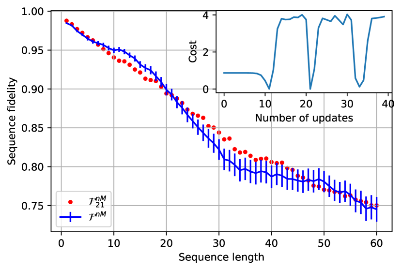
Figure 4: Learned ASF for two qubit fully non-Markovain spin noise model with Adagrad. The blue line is the ASF from the non-Markovian noise model and the error bar is the standard deviation divided by square root of sample numbers. The red dots are the output of our method, obtained by Adagrad with initail learning rate $0.001$. The superscript in $\mathcal{F}^{nM}_{21}$ indicates the noise model and the subscript is the number of iterations to reach this result. The subplot shows the change of cost with iterations, the $21^{\textit{th}}$ iteration gives the ASF data shown in here.

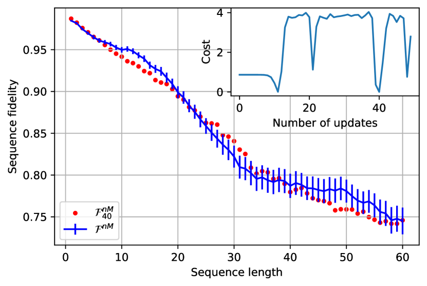
Figure 5: Starting from the $21^{\textit{th}}$ update with different learning rate. The blue line is the ASF from the non-Markovian noise model and the error bar is the standard deviation divided by square root of sample numbers. The red dots are the output of our method, starting with the initial noise from the $21^{\textit{th}}$ update in Fig. 5. The result is obtained by Adagrad with initail learning rate $0.001001$. The superscript in $\mathcal{F}^{nM}_{40}$ indicates the noise model and the subscript is the number of iterations to reach this result. The subplot shows the change of cost with iterations, the $40^{\textit{th}}$ iteration gives the ASF data shown in here.

References

• Emerson et al. [2005] J. Emerson, R. Alicki, and K. Życzkowski, Scalable noise estimation with random unitary operators, J. Opt. B-Quantum S.O. 7, S347 (2005).
• Lévi et al. [2007] B. Lévi, C. C. López, J. Emerson, and D. G. Cory, Efficient error characterization in quantum information processing, Phys. Rev. A 75, 022314 (2007).
• Knill et al. [2008] E. Knill, D. Leibfried, R. Reichle, J. Britton, R. B. Blakestad, J. D. Jost, C. Langer, R. Ozeri, S. Seidelin, and D. J. Wineland, Randomized benchmarking of quantum gates, Phys. Rev. A 77, 012307 (2008).
• Magesan et al. [2011] E. Magesan, J. M. Gambetta, and J. Emerson, Scalable and Robust Randomized Benchmarking of Quantum Processes, Phys. Rev. Lett. 106, 180504 (2011).
• Magesan et al. [2012] E. Magesan, J. M. Gambetta, and J. Emerson, Characterizing quantum gates via randomized benchmarking, Phys. Rev. A 85, 042311 (2012).
• Greenbaum [2015] D. Greenbaum, Introduction to Quantum Gate Set Tomography (2015), arXiv:1509.02921 [quant-ph] .
• Nielsen et al. [2021] E. Nielsen, J. K. Gamble, K. Rudinger, T. Scholten, K. Young, and R. Blume-Kohout, Gate Set Tomography, Quantum 5, 557 (2021).
• Milz and Modi [2021] S. Milz and K. Modi, Quantum Stochastic Processes and Quantum non-Markovian Phenomena, PRX Quantum 2, 030201 (2021).
• Wallman and Flammia [2014] J. J. Wallman and S. T. Flammia, Randomized benchmarking with confidence, New J. Phys. 16, 103032 (2014).
• Helsen et al. [2022] J. Helsen, I. Roth, E. Onorati, A. Werner, and J. Eisert, General framework for randomized benchmarking, PRX Quantum 3, 020357 (2022).
• van Kampen [1998] N. van Kampen, Remarks on Non-Markov Processes, Braz. J. Phys. 2810.1590/s0103-97331998000200003 (1998).
• Figueroa-Romero et al. [2019] P. Figueroa-Romero, K. Modi, and F. A. Pollock, Almost Markovian processes from closed dynamics, Quantum 3, 136 (2019).
• Young et al. [2020] K. Young, S. Bartlett, R. J. Blume-Kohout, J. K. Gamble, D. Lobser, P. Maunz, E. Nielsen, T. J. Proctor, M. Revelle, and K. M. Rudinger, Diagnosing and Destroying Non-Markovian Noise, Tech. Rep. (U.S. Department of Energy, Office of Scientific and Technical Information, 2020).
• Proctor et al. [2020] T. Proctor, M. Revelle, E. Nielsen, K. Rudinger, D. Lobser, P. Maunz, R. Blume-Kohout, and K. Young, Detecting and tracking drift in quantum information processors, Nat. Commun. 11, 5396 (2020).
• Meier [2018] A. M. Meier, Randomized Benchmarking of Clifford Operators (2018), arXiv:1811.10040 [quant-ph] .
• Gottesman [1998] D. Gottesman, The Heisenberg Representation of Quantum Computers (1998), arXiv:quant-ph/9807006 [quant-ph] .
• Gottesman [1997] D. Gottesman, Stabilizer Codes and Quantum Error Correction (1997), arXiv:quant-ph/9705052 [quant-ph] .
• Aaronson and Gottesman [2004] S. Aaronson and D. Gottesman, Improved simulation of stabilizer circuits, Phys. Rev. A 70, 052328 (2004).
• Webb [2016] Z. Webb, The Clifford group forms a unitary 3-design, Quantum Inf. Comput. 16, 1379–1400 (2016).
• Graydon et al. [2021] M. A. Graydon, J. Skanes-Norman, and J. J. Wallman, Clifford groups are not always 2-designs (2021), arXiv:2108.04200 [quant-ph] .
• Figueroa-Romero et al. [2021] P. Figueroa-Romero, K. Modi, R. J. Harris, T. M. Stace, and M.-H. Hsieh, Randomized Benchmarking for Non-Markovian Noise, PRX Quantum 2, 040351 (2021).
• Figueroa-Romero et al. [2022] P. Figueroa-Romero, K. Modi, and M.-H. Hsieh, Towards a general framework of Randomized Benchmarking for non-Markovian Noise (2022), arXiv:2202.11338 [quant-ph] .
• Stoudenmire and Schwab [2016] E. Stoudenmire and D. J. Schwab, Supervised Learning with Tensor Networks, in Adv. Neural Inf. Process. Syst., Vol. 29, edited by D. Lee, M. Sugiyama, U. Luxburg, I. Guyon, and R. Garnett (Curran Associates, Inc., 2016) p. 4799.
• Pollock et al. [2018a] F. A. Pollock, C. Rodríguez-Rosario, T. Frauenheim, M. Paternostro, and K. Modi, Non-Markovian quantum processes: Complete framework and efficient characterization, Phys. Rev. A 97, 012127 (2018a).
• White et al. [2022] G. White, F. Pollock, L. Hollenberg, K. Modi, and C. Hill, Non-markovian quantum process tomography, PRX Quantum 3, 020344 (2022).
• Pollock et al. [2018b] F. A. Pollock, C. Rodríguez-Rosario, T. Frauenheim, M. Paternostro, and K. Modi, Operational Markov Condition for Quantum Processes, Phys. Rev. Lett. 120, 040405 (2018b).
• Milz et al. [2020] S. Milz, F. Sakuldee, F. A. Pollock, and K. Modi, Kolmogorov extension theorem for (quantum) causal modelling and general probabilistic theories, Quantum 4, 255 (2020).
• Taranto et al. [2021] P. Taranto, F. A. Pollock, and K. Modi, Non-Markovian memory strength bounds quantum process recoverability, npj Quantum Inf. 710.1038/s41534-021-00481-4 (2021).
• Milz et al. [2019] S. Milz, M. S. Kim, F. A. Pollock, and K. Modi, Completely Positive Divisibility Does Not Mean Markovianity, Phys. Rev. Lett. 123, 040401 (2019).
• White et al. [2020] G. A. L. White, C. D. Hill, F. A. Pollock, L. C. L. Hollenberg, and K. Modi, Demonstration of non-Markovian process characterisation and control on a quantum processor, Nat. Commun. 1110.1038/s41467-020-20113-3 (2020).
• Nurdin and Gough [2021] H. I. Nurdin and J. Gough, From the heisenberg to the schrödinger picture: Quantum stochastic processes and process tensors, 2021 60th IEEE Conference on Decision and Control (CDC) 10.1109/cdc45484.2021.9683765 (2021).
• White et al. [2021] G. A. L. White, F. A. Pollock, L. C. L. Hollenberg, K. Modi, and C. D. Hill, Non-Markovian Quantum Process Tomography (2021), arXiv:2106.11722 [quant-ph] .
• Watrous [2018] J. Watrous, The Theory of Quantum Information (Cambridge University Press, 2018).
• Luchnikov et al. [2019] I. A. Luchnikov, S. V. Vintskevich, H. Ouerdane, and S. N. Filippov, Simulation Complexity of Open Quantum Dynamics: Connection with Tensor Networks, Phys. Rev. Lett. 122, 160401 (2019).
• Luchnikov et al. [2018] I. A. Luchnikov, S. V. Vintskevich, and S. N. Filippov, Dimension truncation for open quantum systems in terms of tensor networks (2018), arXiv:1801.07418 [quant-ph] .
• Prior et al. [2010] J. Prior, A. W. Chin, S. F. Huelga, and M. B. Plenio, Efficient Simulation of Strong System-Environment Interactions, Phys. Rev. Lett. 105, 050404 (2010).
• Strathearn et al. [2018] A. Strathearn, P. Kirton, D. Kilda, J. Keeling, and B. W. Lovett, Efficient non-Markovian quantum dynamics using time-evolving Matrix Product Operators, Nat. Commun. 910.1038/s41467-018-05617-3 (2018).
• Wall et al. [2016] M. L. Wall, A. Safavi-Naini, and A. M. Rey, Simulating generic spin-boson models with Matrix Product States, Phys. Rev. A 94, 053637 (2016).
• Jørgensen and Pollock [2019] M. R. Jørgensen and F. A. Pollock, Exploiting the Causal Tensor Network Structure of Quantum Processes to Efficiently Simulate Non-Markovian Path Integrals, Phys. Rev. Lett. 123, 240602 (2019).
• Han et al. [2018] Z.-Y. Han, J. Wang, H. Fan, L. Wang, and P. Zhang, Unsupervised generative modeling using matrix product states, Phys. Rev. X 8, 031012 (2018).
• Klus and Gelß [2019] S. Klus and P. Gelß, Tensor-based algorithms for image classification, Algorithms 12, 240 (2019).
• Liu et al. [2019] D. Liu, S.-J. Ran, P. Wittek, C. Peng, R. B. García, G. Su, and M. Lewenstein, Machine learning by unitary tensor network of hierarchical tree structure, New J. Phys. 21, 073059 (2019).
• Araz and Spannowsky [2021] J. Y. Araz and M. Spannowsky, Quantum-inspired event reconstruction with tensor networks: Matrix product states, J. High Energy Phys. 2021 (8).
• Cheng et al. [2021] S. Cheng, L. Wang, and P. Zhang, Supervised learning with projected entangled pair states, Phys. Rev. B 103, 125117 (2021).
• Wang et al. [2021] K. Wang, L. Xiao, W. Yi, S.-J. Ran, and P. Xue, Experimental realization of a quantum image classifier via tensor-network-based machine learning, Photon. Res. 9, 2332 (2021).
• Wall et al. [2021] M. L. Wall, M. R. Abernathy, and G. Quiroz, Generative machine learning with tensor networks: Benchmarks on near-term quantum computers, Phys. Rev. Research 3, 023010 (2021).
• Guo et al. [2020] C. Guo, K. Modi, and D. Poletti, Tensor-network-based machine learning of non-Markovian quantum processes, Phys. Rev. A 102, 062414 (2020).
• Manton [2002] J. Manton, Optimization algorithms exploiting unitary constraints, IEEE Trans. Signal Process. 50, 635 (2002).
• Duchi et al. [2011] J. Duchi, E. Hazan, and Y. Singer, Adaptive subgradient methods for online learning and stochastic optimization, J. Mach. Learn. Res. 12, 2121 (2011).
• Kingma and Ba [2014] D. P. Kingma and J. Ba, Adam: A method for stochastic optimization (2014), arXiv:1412.6980 [cs.LG] .
• Bridgeman and Chubb [2017] J. C. Bridgeman and C. T. Chubb, Hand-waving and interpretive dance: an introductory course on tensor networks, J. Phys. A: Math. Theor. 50, 223001 (2017).
• Barratt et al. [2022] F. Barratt, J. Dborin, and L. Wright, Improvements to gradient descent methods for quantum tensor network machine learning (2022), arXiv:2203.03366 [cs.LG] .
• Muller et al. [2001] K.-R. Muller, S. Mika, G. Ratsch, K. Tsuda, and B. Scholkopf, An introduction to kernel-based learning algorithms, IEEE Trans. Neural Netw. Learn. Syst. 12, 181 (2001).
• Schollwöck [2011] U. Schollwöck, The Density-Matrix Renormalization Group in the age of Matrix Product States, Ann. Phys. 326, 96 (2011).
Glossary
Acronyms
ASF
Average Sequence Fidelity
CP
Completely Positive
CPTP
Completely Positive Trace Preserving
GST
Gate Set Tomography
MPO
Matrix Product Operator
POVM
Positive Operator Valued Measurement
RB
Randomized Benchmarking
SPAM
State Preparation and Measurement
SVD
Singular Value Decomposition