justified [supp:]supplement supplement.pdf

Hydrodynamic description of Non-Equilibrium Radiation

Abstract

Non-equilibrium radiation is addressed theoretically by means of a stochastic lattice-gas model. We consider a resonating transmission line composed of a chain of radiation resonators, each at a local equilibrium, whose boundaries are in thermal contact with two blackbody reservoirs at different temperatures. In the long chain limit, the stationary state of the non-equilibrium radiation is obtained in a closed form. The corresponding spectral energy density departs from the Planck expression, yet it obeys a useful scaling form. A macroscopic fluctuating hydrodynamic limit is obtained leading to a Langevin equation whose transport parameters are calculated. In this macroscopic limit, we identify a local temperature which characterises the spectral energy density. The generality of our approach is discussed and applications for the interaction of non-equilibrium radiation with matter are suggested.

Radiation at thermal equilibrium has been a triggering problem underlying the quantum revolution (Planck, 1900; Einstein, 1917). Since then, this problem has been revisited recurrently in different contexts either in physics or in engineering. Examples are abundant in condensed matter, statistical mechanics and quantum field theory among others (Glauber, 1963; Titulaer and Glauber, 1966; Brańczyk, Chenu, and Sipe, 2017; Kindermann, Nazarov, and Beenakker, 2002).

Radiation out of thermal equilibrium is a problem of wide and obvious interest, yet still largely uncharted despite important advances (Chen, 2000; Joulain et al., 2005; Cleuren and den Broeck, 2007; Biehs, Rousseau, and Greffet, 2010; Bunin et al., 2013; Nicacio et al., 2015; Greffet et al., 2018). The purpose of this letter is to present a hydrodynamic description of non equilibrium radiation. While a wide range of problems can be formulated which involve non equilibrium radiation (Lepri, Livi, and Politi, 2003; Bernard and Doyon, 2012; Xuereb, Imparato, and Dantan, 2015), we focus to the case of two blackbody equilibrium radiation reservoirs held at different temperatures $T_{\mathcal{R}}\neq T_{\mathcal{L}}$ and connected by a properly designed long resonating line of length $L$ as sketched in Fig.1.

Before dwelling into the details of our model, we now summarize our main findings. Non equilibrium radiation is described using a coarse grained, boundary driven, microscopic lattice gas model for the energy transfer along the resonator, which accounts for hopping of photons between neighbouring cells of size $\ell$ $(\ell\ll L)$. We show that this lattice gas model belongs to the well documented zero range process (ZRP) (Evans and Hanney, 2005). The long time probability distribution $P_{\infty}\left(\eta\right)$ of photon configurations is obtained in (10,11). Its continuous limit allows to identify a macroscopic hydrodynamic regime for the steady state akin to the macroscopic fluctuation theory Bertini et al. (2015); Derrida (2007). In this regime, the fluctuating local spectral energy density $u_{\nu}\left(x,t\right)$ is constrained by a continuity equation,

$$\partial_{t}u_{\nu}\left(x,t\right)=-\partial_{x}j(x,t)$$ (1)

where the fluctuating spectral current $j\left(x,t\right)$ obeys the Langevin equation,

$$j\left(x,t\right)=-D\left(\overline{u}_{\nu}\right)\partial_{x}u_{\nu}\left(x,t\right)+\sqrt{\sigma\left(\overline{u}_{\nu}\right)}\,\xi\left(x,t\right)\;.$$ (2)

Here $\xi\left(x,t\right)$ is a weak $(L\gg 1)$ and delta-correlated white noise, $\overline{\xi\left(x,t\right)\xi\left(x^{\prime},t^{\prime}\right)}=\frac{1}{L}\delta\left(x-x^{\prime}\right)\delta\left(t-t^{\prime}\right)$. The transport coefficients,

$$D\left(\overline{u}_{\nu}\right)=\frac{1}{\left(1+\overline{u}_{\nu}\right)^{2}}\,\,\text{and}\;\,\sigma\left(\overline{u}_{\nu}\right)=\frac{2\overline{u}_{\nu}}{1+\overline{u}_{\nu}}\,,$$ (3)

depend solely on the noise-averaged, local spectral energy density $\overline{u}_{\nu}\left(x\right)$ at frequency $\nu$,

$$\overline{u}_{\nu}\left(x\right)\equiv u_{\nu}\left(x\right)/g_{\nu}h\nu\,=\frac{z_{\mathcal{L}}+\frac{x}{L}\left(z_{\mathcal{R}}-z_{\mathcal{L}}\right)}{1-z_{\mathcal{L}}-\frac{x}{L}\left(z_{\mathcal{R}}-z_{\mathcal{L}}\right)}\;,$$ (4)

where $z_{\mathcal{R}/\mathcal{L}}\equiv\exp\left(-h\nu/k_{B}T_{\mathcal{\mathcal{R}}/\mathcal{L}}\right)$ and $g_{\nu}\equiv 8\pi\nu^{2}/c^{3}$ is the $3d$ density of states of the radiation. This expression, very distinct from the Planck distribution, abides the scaling (18) which allows to identify a macroscopic local temperature function $T_{\tau}(x)$ at the hydrodynamic scale. A measurement of local radiation fluxes through apertures along the transmission line akin to standard blackbody measurements is displayed in Fig.1. It provides an experimental way to directly access $u_{\nu}\left(x\right)$ and probe the predicted scaling form and its departure from Planck distribution.

The rest of the letter is devoted to a description of our model and setup, to a derivation of the results just stated and finally, to a discussion of their meaning and applicability.

The Physical Setup – The two blackbody radiation reservoirs in Fig.1 are held at distinct temperatures $T_{\mathcal{R}}\neq T_{\mathcal{L}}$ and are respectively characterised by the Planck distributions, $u_{\nu}\left(T_{r}\right)=g_{\nu}h\nu\left(\mathrm{e}^{\nicefrac{{h\nu}}{{k_{B}T_{r}}}}-1\right)^{-1},\quad{r}=\mathcal{L},\mathcal{R}$ of their spectral energy densities at frequency $\nu$. They are connected by a long transmission line of length $L$ built out of a series of resonators, hereafter cells. In this setup, illustrated in Fig.2, we assume that each cell $k$ of size $\ell$, is large enough so as the enclosed radiation is at thermal equilibrium.

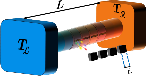
Figure 1: A resonating line connects two blackbody reservoirs held at distinct temperatures $T_{\mathcal{R}}\neq T_{\mathcal{L}}$. The spectral energy density $u_{\nu}(x)$ varies along the line of length $L$. Adopting the standard measurement scheme of $u_{\nu}(x)$, the line is pierced at various locations and an array of detectors of typical size $\ell_{h}$ (see text) records the local non equilibrium spectral radiation $u_{\nu}(x)$.

For $L\gg\ell$, the density of cells is finite and the precise nature of the coupling between neighboring resonators is unimportant. Local thermal equilibrium with the walls (the environment) is achieved through local Kirchhoff law, a point appropriately explored in (Greffet et al., 2018).

The Model – We now outline the assumptions underlying the microscopic lattice model used for the description of the radiation in the transmission line. We consider a one-dimensional lattice $k=1,\dots,N$ of $N=L/\ell$ cells. The left and right blackbody reservoirs are respectively located at $k=0$ and $k=N+1$, so that $T_{\mathcal{L}}\equiv T_{0}$ and $T_{\mathcal{R}}\equiv T_{N+1}$. The radiation consists of a gas of photons occupying the lattice cells and hopping between neighboring cells. This hopping is described by random transitions between cells occupation numbers configurations $\eta=\left\{n_{1},\dots,n_{N}\right\}$, with $n_{k}=0,1,2,\ldots$, i.e $n_{k}$ is unbounded. An example of a configuration is displayed in Fig.2.

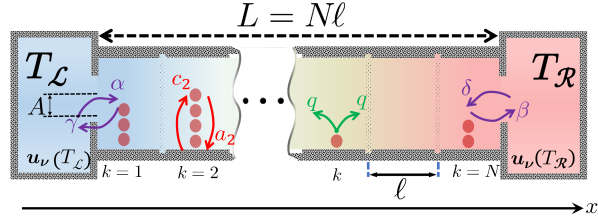
Figure 2: Examples of photon configurations in the lattice model with corresponding transition rates. Each cell $k$ of size $\ell$ accounts for a lattice site, where radiation is locally at thermal equilibrium with surrounding walls. The three processes (1,2,3) namely, in-cell creation and annihilation (red), bulk (green) and boundaries (purple) inter-cell exchanges are indicated.

We denote $\eta_{\overline{i},\underline{j}}\equiv\left\{n_{1},\dots,n_{i}+1,\ldots,n_{j}-1,\ldots,n_{N}\right\}$, $\quad n_{j}>0$, a photon configuration which relatively to $\eta$, has an excess of one photon in the $i^{\mathrm{th}}$ cell and a depletion of one photon in cell $j$. For the bulk and boundary cells we consider the three following processes:

1. Creation/annihilation: $\eta\xrightleftharpoons[a_{k}\left(n_{k}+1\right)]{c_{k}\left(n_{k}\right)}\eta_{\overline{k}}$ photons are absorbed at the boundaries of the $k^{\text{th}}$ cell at a rate $a_{k}$ and created at a rate $c_{k}$. These rates depend on $n_{k}$ and we set $a_{k}=0$ for $n_{k}=0$ for all $k$. Furthermore, these rates are constrained by local detailed balance (12) within each cell $k$.

2. Bulk exchange: $\eta_{\overline{k},k+1}\xrightleftharpoons[q]{q}\eta_{k,\overline{k+1}}$, namely the hopping of photons between neighboring cells is symmetric and occurs at a rate $q$. We shall set $q=1$ in the sequel.

3. Boundary processes – At the boundary cells $k=1$ and $k=N$, we assign:

   • $\eta\xrightleftharpoons[\gamma]{\alpha}\eta_{\overline{1}}$ : The left reservoir respectively absorbs and injects photons from/into the transmission line at rates $\gamma$ and $\alpha$.

   • $\eta\xrightleftharpoons[\beta]{\delta}\eta_{\overline{N}}$ : The right reservoir respectively absorbs and injects photons from/into the transmission line at rates $\beta$ and $\delta$.

Physically, the rates $\alpha$ and $\delta$ express the radiation fluxes from the reservoir into the transmission line through small apertures of area $A$, namely, $\alpha=2A\,c\,u_{\nu}\left(T_{0}\right)/h$ and $\delta=2A\,c\,u_{\nu}\left(T_{N+1}\right)/h$ (see Fig.2 and Supplemental Material S I (sup, )).

The three processes $(1,2,3)$ listed above, underlie the dynamics of non equilibrium radiation states by means of the probability $P_{t}\left(\eta\right)$ for a configuration $\eta$ of photons at time $t$. This dynamics of configurations is thus given by solutions of a master equation, $\partial_{t}P_{t}\left(\eta\right)=\mathcal{L}\left[P_{t}\left(\eta\right)\right]$ where the generator $\mathcal{L}$, linear in $P_{t}$, specifies the rate of probability flow between occupation configurations. We are interested in the form of the long time probability $P_{\infty}\left(\eta\right)\equiv\lim_{t\rightarrow\infty}P_{t}\left(\eta\right)$, namely in the solutions of the kernel equation,

$$\mathcal{L}\left[P_{\infty}\left(\eta\right)\right]=0\,.$$ (5)

Since the processes $(1)$ and $(2+3)$ are independent, we look for solutions with independent generators,

$$\mathcal{L}\equiv\mathcal{L}^{\perp}+\mathcal{L}^{\parallel}$$ (6)

where $\mathcal{L}^{\perp}$ accounts for process $(1)$ and $\mathcal{L}^{\parallel}\equiv\mathcal{L}_{\text{bulk}}+\mathcal{L}_{\text{boundary}}$ accounts for processes $(2)$ and $(3)$. Expressions of these generators are given in the Supplementary Material S IV in (sup, ). To evaluate the kernel of $\mathcal{L}^{\parallel}$, we consider the statistics of the total current $Q_{t}$ of independent photons hopping on the lattice, and removed and injected from the boundary blackbody reservoirs at rates ($\alpha,\beta,\gamma,\delta$) during the time interval $[0,t]$. We define the cumulant generating function $\langle\mathrm{e}^{\lambda Q_{t}}\rangle$ of $Q_{t}$, the average $\langle\cdots\rangle$ being on the Poisson processes governing the time-dependent boundary dynamics (S II in (sup, )). In the long time limit, we expect $\langle\mathrm{e}^{\lambda Q_{t}}\rangle\simeq\mathrm{e}^{\mu^{\parallel}(\lambda)t}$. Hence, the knowledge of $\mu^{\parallel}(\lambda)$ allows to obtain the cumulants of $Q_{t}$ by

$$\lim_{t\rightarrow\infty}\frac{\langle Q_{t}^{n}\rangle_{c}}{t}=\frac{\mathrm{d}^{n}\mu(\lambda)}{\mathrm{d}\lambda^{n}}|_{\lambda=0}\,.$$ (7)

To compute $\mu^{\parallel}(\lambda)$, we rely on the assumption that photons are independent, which allows to study separately the effect of right and left reservoirs. The number of photons leaving the transmission line from its left boundary in the time interval $[0,t]$ is,

$$Q^{\mathcal{L}}_{[0,t]}=\overrightarrow{{\bf 1}}_{[0,t]}-\overleftarrow{{\bf 1}}_{[0,t]}$$ (8)

where $\overrightarrow{{\bf 1}}_{[0,t]}$ (resp. $\overleftarrow{{\bf 1}}_{[0,t]}$) is the number of photons leaving (resp. entering) the left reservoir to (resp. from) cell ${\bf 1}$ in the time interval $[0,t]$. Since photons are independent, we decompose the total current by partitioning the time interval $[0,t]$ into $N_{t}$ segments $[t_{k},t]$ with $t_{k}$ being the time at which the $k^{\text{th}}$ photon entered the system. The total current $Q^{\mathcal{L}}_{[0,t]}$ then appears as the sum of elementary contributions of each photon that has entered the resonator between times $0$ and $t$, $Q^{\mathcal{L}}_{[0,t]}=\sum_{k=0}^{N_{t}}Q^{k}_{[t_{k},t]}$. This partition simplifies the calculation of the left part of the cumulant generating function $\mu_{\mathcal{L}}(\lambda)=\lim_{t\rightarrow\infty}\frac{1}{t}\ln\langle e^{\lambda Q^{\mathcal{L}}_{[0,t]}}\rangle$ by factorising it into a product of single photon contributions (see S II in (sup, ) for details). A similar calculation for the current $Q^{\mathcal{R}}_{[0,t]}$ of photons leaving the transmission line from its right boundary and the corresponding generating function $\mu_{\mathcal{R}}(\lambda)$ leads to (sup, ),

$$\mu^{\parallel}(\lambda)=\mu_{\mathcal{L}}-\mu_{\mathcal{R}}=\frac{\alpha\beta(e^{\lambda}-1)-\gamma\delta(1-e^{-\lambda})}{\gamma(\beta N+1)-\beta(\gamma-1)}\,.$$ (9)

The generating function $\mu^{\parallel}(\lambda)$ coincides with those describing the dynamics of a class of stochastic lattice gas models known as the zero-range-process (ZRP) (Harris, Rákos, and Schütz, 2005). This result is not obvious since, unlike our model, the ZRP describes interacting particles. Yet, based on this identity, we use the result, proven for ZRP (Levine, Mukamel, and Schütz, 2005), that the long time probability $P_{\infty}\left(\eta\right)$ solution of $\mathcal{L}^{\parallel}\left[P_{\infty}\left(\eta\right)\right]=0$ in (5), is a product measure, namely,

$$P_{\infty}\left(\eta\right)=\prod_{k=1}^{N}\pi_{k}\left(n_{k}\right)\,.$$ (10)

Each term $\pi_{k}\left(n_{k}\right)$ accounts for the bookkeeping of photon occupation number in cell $k$ at local equilibrium, and it is expressed in terms of the steady state fugacities $z_{k}$,

$$\pi_{k}\left(n_{k}\right)=\left(1-z_{k}\right)z_{k}^{n_{k}}\,.$$ (11)

Under this form, a sufficient condition for local equilibrium is expressed by a detailed balance condition,

$$\frac{c_{k}\left(n_{k}\right)}{a_{k}\left(n_{k}+1\right)}=\frac{P_{\infty}\left(\eta_{\overline{k}}\right)}{P_{\infty}\left(\eta\right)}=z_{k}\,.$$ (12)

Expressions (11) and (12) generalize the condition for thermal blackbody radiation with fugacity $z^{B}=\exp\left(-{h\nu}/{k_{B}T}\right)$ (sup, ). It is immediate to check that (11) implies $\mathcal{L}^{\perp}\left[P_{\infty}\left(\eta\right)\right]=0$. Hence (5) amounts to solutions of $\mathcal{L}^{\parallel}\left[P_{\infty}\left(\eta\right)\right]=\mathcal{L}_{\text{ZRP}}\left[P_{\infty}\left(\eta\right)\right]=0$ characterised by fugacities (Levine, Mukamel, and Schütz, 2005; sup, ),

$$z_{k}=\frac{\frac{k}{N}\left(\gamma\delta-\alpha\beta\right)+\alpha\beta-\frac{1}{N}\left[\gamma\delta+\left(\alpha+\delta\right)\right]}{\beta\gamma\left(1-\frac{1}{N}\right)+\frac{1}{N}\left(\beta+\gamma\right)}\,.$$ (13)

Fugacities in the blackbody reservoirs are given by $z_{\mathcal{L}/\mathcal{R}}\equiv z_{{0}/{N+1}}=\exp\left(-h\nu/k_{B}T_{\mathcal{L}/\mathcal{R}}\right)$. Taking the large $N$ limit in (13) leads to the boundary conditions (Derrida, 2007),

$$z_{0}=\mathrm{e}^{-\frac{h\nu}{k_{B}T_{\mathcal{L}}}}=\frac{\alpha}{\gamma},\qquad z_{N+1}=\mathrm{e}^{-\frac{h\nu}{k_{B}T_{\mathcal{R}}}}=\frac{\delta}{\beta}\;,$$ (14)

, so that (9) rewrites,

$$\mu^{\parallel}(\lambda)=\frac{1}{L}\left(1-\mathrm{e}^{-\lambda}\right)\left(z_{\mathcal{L}}\,\mathrm{e}^{\lambda}-z_{\mathcal{R}}\right)\,.$$ (15)

Boundary conditions (14) can also be obtained in a different way if one notes that $\mu^{\parallel}(\lambda)$ in (15) abides the Gallavotti and Cohen relation (Gallavotti and Cohen, 1995; Lebowitz and Spohn, 1998),

$$\mu^{\parallel}(\lambda)=\mu^{\parallel}(-\lambda-E)$$ (16)

where $E$ is a field that brings the radiation out of equilibrium. Taking $E\equiv\ln z_{\mathcal{R}}-\ln z_{\mathcal{L}}$, corresponds to (14).

To establish (4) for the spectral energy density $u_{\nu}\left(x\right)$, we now consider the hydrodynamic continuous limit obtained by averaging over cell sizes $\ell$. Namely, defining $k\ell/L=k/N\equiv x\;\left(0\leq x\leq 1\right)$, with $L\rightarrow\infty$, $\ell\rightarrow\infty$, and keeping a finite density of cells $\ell/L\rightarrow\text{d}x$. This averaging procedure , applied to the fugacity in (13) gives,

$$z_{k}\rightarrow z\left(x\right)=\frac{\alpha}{\gamma}+x\left(\frac{\delta}{\beta}-\frac{\alpha}{\gamma}\right)=z_{\mathcal{L}}+x\left(z_{\mathcal{R}}-z_{\mathcal{L}}\right)\,.$$ (17)

The spectral energy density of the radiation at frequency $\nu$ in cell $k$ inside the transmission line is $u_{\nu}\left(k\right)=g_{\nu}h\nu\left\langle n_{k}\right\rangle$ with $\left\langle n_{k}\right\rangle=\sum_{\eta}n_{k}P_{\infty}\left(\eta\right)=z_{k}/(1-z_{k})$. In the continuous limit, $\left\langle n\left(x\right)\right\rangle=\frac{z\left(x\right)}{1-z\left(x\right)}$ leads to (4) for the macroscopic spectral energy density $u_{\nu}\left(x\right)$ as announced in the introductory part.

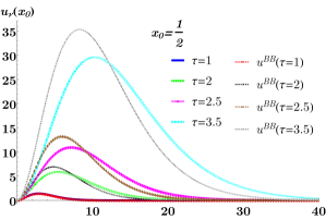
(a)

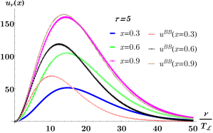
(b)

Figure 3: Behaviour of $u_{\nu}\left(x\right)$ in (4) - Difference with the Planck spectral distribution. (a) $u_{\nu}\left(x=1/2\right)$, plotted as a function of $\nu/T_{\mathcal{L}}$ for different values of the ratio $\tau\equiv T_{\mathcal{R}}/T_{\mathcal{L}}$. The Planck distribution $u^{B}$ for the same temperature function $T_{\tau}(\frac{1}{2})$ is plotted for comparison. The difference between the two functions appears clearly except for $\tau=1$. (b) Same plots but for different positions $x$ and for a fixed ratio $\tau\equiv T_{\mathcal{R}}/T_{\mathcal{L}}=5$.

Expression (4) manifestly differs from the Planck spectral energy density, a direct consequence of the non equilibrium nature of the radiation at the macroscopic scale. This difference is illustrated in Fig. 3a for different values of the ratio $\tau\equiv T_{\mathcal{R}}/T_{\mathcal{L}}$ and at a fixed position along the transmission line. The same observation holds for a fixed value $\tau\neq 1$ while varying the position $x$ along the line (Fig.3b).

A remarkable scaling form,

$$u_{\nu}\left(x\right)\equiv\frac{8\pi h}{c^{3}}\nu^{3}\Phi\left(\nu/T_{\tau}(x)\right)$$ (18)

for $u_{\nu}\left(x\right)$ is observed in Fig.4 where the function $T_{\tau}(x)$, a temperature, is to be determined. It is interesting to note that while $u_{\nu}\left(x\right)$ is not a Planck distribution for $\tau\neq 1$, the scaling form (18) implies $\int\mathrm{d}\nu\,u_{\nu}\left(x\right)\propto T_{\tau}^{4}(x)$, a behaviour reminiscent of the thermodynamic result. To understand these results and to determine the temperature $T_{\tau}(x)$, we now propose a fluctuating hydrodynamic description.

In the limit $L\rightarrow\infty$, upon rescaling space, $x\rightarrow x/L$ and time, $t\rightarrow t/L^{2}$, the evolution of the stochastic model (9,10) can be described using a fluctuating hydrodynamic Langevin equation (2) relating a current density $j(x,t)$ to the fluctuating local spectral energy density $u_{\nu}\left(x,t\right)$, both being constrained by the continuity equation (1).

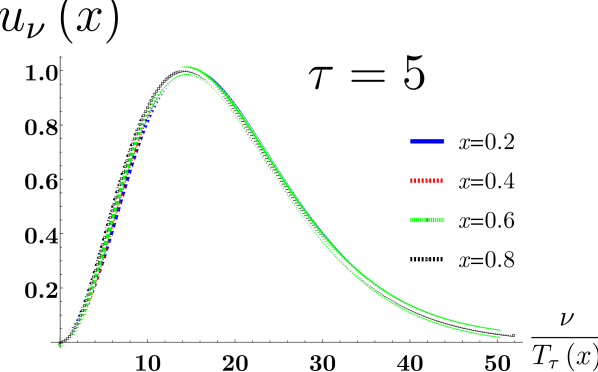
Figure 4: Scaling form (18) for $u_{\nu}\left(x\right)$. All curves evaluated at a fixed temperature ratio $\tau=\frac{T_{\mathcal{R}}}{T_{\mathcal{L}}}=5$ but for different values $x$ of the position, collapse to a single curve upon a proper rescaling $\nu/T_{\tau}\left(x\right)$ thus defining the temperature function $T_{\tau}(x)$.

The validity of this fluctuating hydrodynamic description, a.k.a macroscopic fluctuation theory (MFT) (Bertini et al., 2015), relies on the assumption of local equilibrium around each cell $\ell$ at an intermediate hydrodynamic scale $(\ell\ll\ell_{h}\ll L)$ and for times much larger than $\ell_{h}^{2}$ and much smaller than $L^{2}$, where the spectral energy density is $u_{\nu}\left(x\right)$ given in (4). This assumption implies that only linear response coefficients $D\left(\overline{u}_{\nu}\right)$ and $\sigma\left(\overline{u}_{\nu}\right)$ show up in the Langevin equation (2). To calculate them, we use the cumulant generation function $\mu^{\parallel}(\lambda)$ in (15) of the total radiation current

$$Q_{t}=\frac{L^{2}}{t}\int_{0}^{t}dt^{\prime}\int_{0}^{1}dx\,j(x,t^{\prime})$$ (19)

transferred between the reservoirs in a time window $\left[0,t\right]$. To calculate the transport coefficients $\sigma\left(\overline{u}_{\nu}\right)$ and $D\left(\overline{u}_{\nu}\right)$ in (3), we note that the Gallavotti and Cohen relation (16) generalises local detailed balance conditions (12) and allows to recover the fluctuation-dissipation theorem in the limit $E\rightarrow 0$. Hence, expanding the generating function $\mu^{\parallel}(\lambda)$ close to equilibrium, i.e. for $\tau\simeq 1$ and by setting $u_{\mathcal{L}}\equiv u,\,u_{\mathcal{R}}\equiv u+\Delta u$ with $\Delta u\ll 1$, leads to,

$$\frac{\left\langle Q(t)\right\rangle}{t}= \frac{\mathrm{d}\mu^{\parallel}(\lambda)}{\mathrm{d}\lambda}|_{\lambda=0}\equiv D\left(u\right)\frac{\Delta u}{L}$$ (20a)

$$\frac{\left\langle Q^{2}(t)\right\rangle}{t}= \frac{\mathrm{d}^{2}\mu^{\parallel}(\lambda)}{\mathrm{d}\lambda^{2}}|_{\lambda=0}\equiv\frac{\sigma\left(u\right)}{L}\;.$$ (20b)

The resulting expressions (3) for $D\left(\overline{u}_{\nu}\left(x\right)\right)$ and $\sigma\left(\overline{u}_{\nu}\left(x\right)\right)$ coincide with those established for the ZRP (De Masi and Ferrari, 1984; Landim and Mourragui, 1997; Schütz and Harris, 2007; Hirschberg, Mukamel, and Schütz, 2015) (S V of (sup, )). An elementary consequence (Derrida, 2007) of the generalised detailed balance relation (16), implies that they abide the Einstein relation,

$$\frac{2D\left(\overline{u}_{\nu}\right)}{\sigma\left(\overline{u}_{\nu}\right)}=-\,\overline{s}_{\nu}^{\prime\prime},$$ (21)

relating $D$ and $\sigma$ to the second derivative of the local spectral entropy density $\overline{s}_{\nu}\left(\overline{u}_{\nu}(x)\right)\equiv s_{\nu}/\frac{8\pi k_{B}\nu^{2}}{c^{3}}$ with respect to $\overline{u}_{\nu}$.

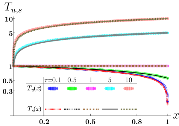
Figure 5: Comparison between the temperatures $T_{u}$ and $T_{s}$ defined from the energy and entropy densities $u(x)$ and $s(x)$, as functions of the location $x$ along the transmission line.

Einstein relation (21) is useful since it allows to calculate $s_{\nu}(x)$ by a direct integration and using (18). This leads to

$$s_{\nu}(x)=-\frac{8\pi k_{B}}{c^{3}}\nu^{2}\left[\left(1+\Phi\right)\ln\left(1+\Phi\right)-\Phi\ln\Phi\right]\,.$$ (22)

Since $\Phi$ depends only on the argument $\nu/T_{\tau}(x)$, then $s(x)=\int_{0}^{\infty}\mathrm{d}\nu\,s_{\nu}(x)=A_{s}T_{s}^{3}(x)$, where $A_{s}$ is a constant which depends on $\Phi$. The scaling form (18) implies $u(x)=\int_{0}^{\infty}\mathrm{d}\nu\,u_{\nu}(x)=A_{u}\,T_{u}^{4}(x)$, where $A_{u}$ is another constant which depends on $\Phi(x)$. From these two relations, we recover the familiar thermodynamic relation $\partial s(x)/\partial u(x)\propto 1/T_{\tau}(x)$, so that $T_{\tau}(x)$ is indeed a local temperature . This result has been checked numerically in Fig.5 where the two temperatures $T_{u}$ and $T_{s}$, respectively retrieved from $u_{\nu}(x)$ in (18) and from $s_{\nu}(x)$ in (22), are shown to coincide and to be equal to $T_{\tau}(x)$.

To summarize our findings, we have proposed a macroscopic hydrodynamic description of non equilibrium radiation. We have considered the workable example where the radiation is driven out of equilibrium by thermal coupling to two blackbody reservoirs at different temperatures. Yet, the generality of our findings appears to be independent of this specific model. We have shown that our boundary driven lattice gas model based on the bookkeeping of local photon exchanges, shares the universality of the ZRP model (Levine, Mukamel, and Schütz, 2005; De Masi and Ferrari, 1984; Schütz and Harris, 2007; Hirschberg, Mukamel, and Schütz, 2015). Moreover, a useful macroscopic hydrodynamic limit described by the Langevin equation (2) has been obtained which depends on two transport parameters $D(u_{\nu})$ and $\sigma(u_{\nu})$ only. These results constitute an additional contribution to an already abundant literature on stationary, out of equilibrium, boundary driven systems (Landim and Mourragui, 1997; Bertini et al., 2006; Harris, Rákos, and Schütz, 2005; Hirschberg, Mukamel, and Schütz, 2015). In the present case, the starting point of our study is a rather general scheme for non equilibrium photon propagation which could be further extended to other sources of fluctuating light either coherent or incoherent (e.g. lasers). Our results constitute a starting point to study more complicated situations such as the action of non equilibrium radiation on atomic motion (e.g. optical tweezers or atomic cooling), or the dynamics of quantum entanglement between two quantum particles interacting with non equilibrium light. Dynamical phase transitions and the existence of some form of condensation in the ZRP are interesting directions worth pursuing. Another interesting question is the control of fluctuating quantities in the hydrodynamic description, e.g. by means of ”Thermodynamic Uncertainty Relation” recently proposed (Barato and Seifert, 2015).

See pages 1, of supplement.pdf See pages 0, of supplement.pdf

References

- Planck (1900) M. Planck, Verh. Deut. Phys. Ges 2, 237 (1900).
- Einstein (1917) A. Einstein, Verh. Deut. Phys. Ges. 13, 318 (1917).
- Glauber (1963) R. J. Glauber, Phys. Rev. 131, 2766 (1963).
- Titulaer and Glauber (1966) U. M. Titulaer and R. J. Glauber, Phys. Rev. 145, 1041 (1966).
- Brańczyk, Chenu, and Sipe (2017) A. M. Brańczyk, A. Chenu, and J. E. Sipe, J. Opt. Soc. Am. B 34, 1536 (2017).
- Kindermann, Nazarov, and Beenakker (2002) M. Kindermann, Y. V. Nazarov, and C. W. J. Beenakker, Phys. Rev. Lett. 88, 063601 (2002).
- Chen (2000) G. Chen, Journal of Nanoparticle Research 2, 199 (2000).
- Joulain et al. (2005) K. Joulain, J. P. Mulet, F. Marquier, R. Carminati, and J. J. Greffet, Surface Science Reports 57, 59 (2005).
- Cleuren and den Broeck (2007) B. Cleuren and C. den Broeck, Epl 79, 30001 (2007).
- Biehs, Rousseau, and Greffet (2010) S. A. Biehs, E. Rousseau, and J. J. Greffet, Physical Review Letters 105, 3 (2010).
- Bunin et al. (2013) G. Bunin, Y. Kafri, V. Lecomte, D. Podolsky, and A. Polkovnikov, Journal of Statistical Mechanics: Theory and Experiment 2013, P08015 (2013).
- Nicacio et al. (2015) F. Nicacio, A. Ferraro, A. Imparato, M. Paternostro, and F. L. Semião, Physical Review E - Statistical, Nonlinear, and Soft Matter Physics 91 (2015), 10.1103/PhysRevE.91.042116.
- Greffet et al. (2018) J. J. Greffet, P. Bouchon, G. Brucoli, and F. Marquier, Physical Review X 8, 21008 (2018).
- Lepri, Livi, and Politi (2003) S. Lepri, R. Livi, and A. Politi, Physics Reports 377, 1 (2003).
- Bernard and Doyon (2012) D. Bernard and B. Doyon, Journal of Physics A: Mathematical and Theoretical 45, 362001 (2012).
- Xuereb, Imparato, and Dantan (2015) A. Xuereb, A. Imparato, and A. Dantan, New Journal of Physics 17 (2015), 10.1088/1367-2630/17/5/055013.
- Evans and Hanney (2005) M. R. Evans and T. Hanney, J. Phys. A: Math. Gen. 38 (2005), 10.1088/0305-4470/38/19/R01.
- Bertini et al. (2015) L. Bertini, A. De Sole, D. Gabrielli, G. Jona-Lasinio, and C. Landim, Reviews of Modern Physics 87, 593 (2015).
- Derrida (2007) B. Derrida, J. Stat. Mech. 07023, P07023 (2007).
- (20) Suplementary material is available at URL_will_be_inserted_by_publisher.
- Harris, Rákos, and Schütz (2005) R. J. Harris, A. Rákos, and G. M. Schütz, Journal of Statistical Mechanics: Theory and Experiment , 55 (2005).
- Levine, Mukamel, and Schütz (2005) E. Levine, D. Mukamel, and G. M. Schütz, J. Stat. Phys. 120, 759 (2005).
- Note (1) Having imposes and .
- Gallavotti and Cohen (1995) G. Gallavotti and E. G. D. Cohen, Physical Review Letters 74, 2694 (1995).
- Lebowitz and Spohn (1998) J. L. Lebowitz and H. Spohn, Journal of Statistical Physics , 333 (1998).
- De Masi and Ferrari (1984) A. De Masi and P. Ferrari, Journal of statistical physics 36, 81 (1984).
- Landim and Mourragui (1997) C. Landim and M. Mourragui, Annales de l’institut Henri Poincare (B) Probability and Statistics 33, 65 (1997).
- Schütz and Harris (2007) G. M. Schütz and R. J. Harris, Journal of Statistical Physics 127, 419 (2007).
- Hirschberg, Mukamel, and Schütz (2015) O. Hirschberg, D. Mukamel, and G. M. Schütz, Journal of Statistical Mechanics: Theory and Experiment 2015, P11023 (2015).
- Note (2) The proportionality constant is , i.e . See S\tmspace+.1667emVI of (sup, ) for the proof of the relation . In contrast, at equilibrium, , the constants are , such that .
- Bertini et al. (2006) L. Bertini, A. De Sole, D. Gabrielli, G. Jona-Lasinio, and C. Landim, Journal of Statistical Physics 123, 237 (2006).
- Barato and Seifert (2015) A. C. Barato and U. Seifert, Phys. Rev. Lett. 114, 158101 (2015).