Spacetime Entanglement Entropy:
Covariance and Discreteness

Abstract

We review some recent results on Sorkin’s spacetime formulation of the entanglement entropy (SSEE) for a free quantum scalar field both in the continuum and in manifold-like causal sets. The SSEE for a causal diamond in a 2d cylinder spacetime has been shown to have a Calabrese-Cardy form, while for de Sitter and Schwarzschild de Sitter horizons in dimensions $d>2$, it matches the mode-wise von-Neumann entropy. In these continuum examples the SSEE is regulated by imposing a UV cut-off. Manifold-like causal sets come with a natural covariant spacetime cut-off and thus provide an arena to study regulated QFT. However, the SSEE for different manifold-like causal sets in $d=2$ and $d=4$ has been shown to exhibit a volume rather than an area law. The area law is recovered only when an additional UV cut-off is implemented in the scaling regime of the spectrum which mimics the continuum behaviour. We discuss the implications of these results and suggest that a volume-law may be a manifestation of the fundamental non-locality of causal sets and a sign of new UV physics.

1 Introduction

It is now well established that entanglement entropy (EE) is a useful tool for measuring both the entanglement between subsystems as well as accounting for the Entropy-Area law in a diverse range of systems, including black holes and other spacetimes with horizons [1]. Unlike the classical entropy associated with a box of gas which is extensive, the EE is expected to satisfy complementarity, which in turn implies that the entanglement is localised to the boundary separating the system from its environment. More broadly, this is true of local QFTs with UV fixed points. While this may seem to be a general, and even defining picture of EE (thus linking it naturally to holography [2]), it is only a part of the story. The EE for systems with long range interactions or which are non-local do not necessarily satisfy an area law. In [3] the EE for subsystems in long-range Ising and Kitaev models were seen to follow either a volume law or an area law depending on the exponent $\alpha$ in the fall off $r^{-\alpha}$. Volume laws have also been shown for non-local QFTs like non-commutative field theories as well as scalar QFT with non-local interactions on a lattice [4, 5, 6]. These provide interesting counter-examples to many of the standard discussions on area laws and complementarity of the von-Neumann entropy. In particular, taking our cue from condensed matter systems where this has been related to quantum phases [3, 6, 7] and the absence of conformal invariance, it seems pertinent to revisit our assumptions about the nature of microscopic black hole area laws.

Since the finiteness of the EE in a QFT depends on the UV cut-off, a starting point would be to ask whether there are hidden assumptions about the UV behaviour of the QFT. In the standard calculations it is assumed that a change in the cut-off $l_{c}$ only serves to rescale the units in which the area is measured, i.e. that $\ln(S_{EE})=-(d-2)\ln l_{c}+b$. Given the experience from condensed matter systems this is perhaps too strong an assumption for a theory of quantum gravity, especially one in which non-locality might play an important role, as suggested in [6].

Without a complete theory of quantum gravity, this may seem hopelessly speculative. However, since the EE for a QFT is calculated in a regime in which one still has a separation between the field and the background spacetime, we can study the EE of QFT on models of quantum gravity inspired spacetime, which are UV complete. Causal set theory provides us with one such concrete example, where the continuum spacetime is replaced by an ensemble of randomly generated locally finite posets or causal sets, with the order relation corresponding to the spacetime causal relation. This picture of spacetime is motivated by the Hawking-King-McCarthy-Malament theorem, which says that the causal structure poset of distinguishing spacetimes determines its conformal class [8, 9].

The random discretisation of spacetime provided by causal sets theory is thus a useful arena in which to test these ideas. Despite being discrete, causal sets do not violate local Lorentz invariance and provide a fundamental covariant spacetime cut-off. The free scalar QFT on manifold like causal sets was first studied in $d=2$ and $d=4$ Minkowski spacetime starting from the Green’s function [10]. Because of the combination of discreteness and covariance in a causal set, Cauchy hypersurfaces are ill-defined and hence so are equal-time commutation relations. These can however be replaced by the covariant Peierls bracket, which as shown by Jonhston [11] provides a novel route to quantisation via whats now called the Sorkin-Johnston (SJ) vacuum [12, 13, 14, 15].

Since standard calculations of the EE also require Cauchy hypersurfaces, one needs a spacetime formulation of the EE for causal sets. Sorkin’s spacetime entanglement entropy (SSEE) formulation for Gaussian free scalar fields provides an alternative measure for entanglement in terms of spacetime correlators [16]. In the continuum the SSEE has been calculated for different types of horizons, in $d\geq 2$ and shown to satisfy the expected area law behaviour [17, 18, 19]. On a causal set the SSEE can be calculated using the SJ vacuum, given the discrete Green’s function. Sorkin and Yazdi first calculated the SSEE in causal sets approximated by a pair of nested $d=2$ Minkowski causal diamonds [20] and more recently it has been calculated for $d=2,4$ de Sitter horizons as well as nested causal diamonds in $d=4$ Minkowski spacetime. In all cases, the SSEE for the causal set exhibits a volume rather than an area law. As shown by Sorkin and Yazdi, the area law is recovered only when an additional UV truncation is imposed on the SJ spectrum in the part of the spectrum that exhibits a continuum-like scaling-behaviour. Fig 1 shows the comparison of the continuum SJ spectrum with the causal set spectrum for different discreteness scales.

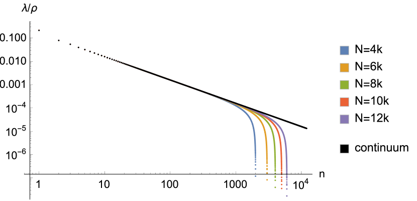
Figure 1: A log-log plot of the SJ spectrum wavelength $\lambda$ versus quantum number $n$. The black solid line is the continuum spectrum which exhibits a scale invariance. The coloured plots are the causal set spectrum for different discreteness scales which mimics the continuum scale invariance upto a “knee” beyond which it is explicitly broken.

As shown in [21] the observations of [20] for the $d=2$ nested causal diamonds hold more generally for the de Sitter case as well. This general behaviour in all these cases can be related to some gross common features in the the causal set SJ spectrum. For small quantum number $n$ the spectrum has a continuum-like scaling regime $\lambda\propto n^{-\alpha}$ which develops into a linear regime $\lambda\propto n$ in the far UV.

In Section 2 we review the construction of the SSEE [16]. In Section 3 we discuss results in the the continuum which show that the SSEE gives the expected area laws for $d>2$ de Sitter and Schwarzschild-de Sitter horizons [19]. For the $d=2$ causal diamond in the cylinder spacetime the Calabrese-Cardy form for the EE is recovered, but the coefficients are not universal [18]. In Section 4 we summarise results on the causal set SSEE volume law as well as the truncation dependent area law [20, 21]. We analyse the SJ spectrum and show that it follows a scaling-behaviour which then transitions to a linear behaviour in the UV. In Section 5 we end with a brief discussion of our results.

2 Sorkin’s Spacetime Entanglement Entropy

In a manifold-like causal set non-locality implies that while there are analogs of spacelike hypersurfaces, these cannot in any sense be Cauchy. In order to define and study the EE of QFT on causal sets therefore one needs a spacetime approach to quantisation and additionally a spacetime formulation of the EE.

For a free Gaussian scalar field, and for a compact region of spacetime or equivalently for a finite causal set, such a spacetime quantisation is possible via the Sorkin-Johnston formulation. Sorkin’s spacetime Entanglement Entropy (SSEE) formula in terms of field correlators then gives us the requisite form of the EE for causal sets. We describe these constructions below. Note that in all that follows we assume a free Gaussian scalar field, and unless specified otherwise, compact spacetime regions.

The alternative to equal time commutation relations is the Peierel’s bracket

$$[\phi(x),\phi(x^{\prime})]=i\Delta(x,x^{\prime})$$ (2.1)

where the Pauli-Jordan operator $\Delta(x,x^{\prime})=G_{R}(x,x^{\prime})-G_{A}(x,x^{\prime})$. In [11] this was used as a starting point for defining a free scalar field Quantum Field Theory on a manifold-like causal set for which the advanced and retarded Green functions $G_{A,R}(x,x^{\prime})$ are known. We describe this “Sorkin-Johnston” approach to defining the free scalar field Quantum Field Theory, first in the continuum and then subsequently in the causal set where it was first discovered [10].

For a compact globally hyperbolic spacetime region $(M,g)$ the integral operator

$$i\widehat{\Delta}\circ\psi(x)\equiv i\int dV^{\prime}\Delta(x,x^{\prime})\psi(x^{\prime})$$ (2.2)

is self-adjoint. Since $\mathrm{ker}\Box=\mathrm{Im}\Delta$, the eigenbasis of $i\widehat{\Delta}$, which we call the Sorkin-Johnston (SJ) basis, provides a unique and covariant mode decomposition for the quantum field. The spectral decomposition of $i\widehat{\Delta}$ in terms of the SJ basis is

$$i\Delta(x,x^{\prime})=\sum_{k}\lambda_{k}u_{k}(x)u_{k}^{*}(x^{\prime})-\sum_{k}\lambda_{k}u_{k}^{*}(x)u_{k}(x^{\prime})$$ (2.3)

where we have used the fact that the SJ eigenvalues come in pairs $(\lambda_{k},-\lambda_{k})$ with corresponding eigenfunctions $(u_{k}(x),u_{k}^{*}(x))$, $\lambda_{k}>0$. The novel insight in [11] was the recognition that this suffices to define the Wightman function, and hence a covariant quantum vacuum, i.e.

$$W_{\text{SJ}}(x,x^{\prime})=\mathrm{Pos}(i\Delta)(x,x^{\prime})=\sum_{k}\lambda_{k}u_{k}(x)u_{k}^{*}(x^{\prime}).$$ (2.4)

This SJ vacuum has been extensively studied both in the continuum and in causal sets, where it was first obtained [11, 12, 13, 22, 14, 15, 23, 24, 25].

In studying the EE of quantum fields, one typically looks at entanglement between a spatial region $U_{\Sigma}$ on a Cauchy hypersurface $\Sigma$ and its complement $U_{\Sigma}^{c}$ in $\Sigma$. However, there is a more natural underlying spacetime picture of entanglement, commonly used in AQFT, which is an entanglement between the spacetime regions $D(U_{\Sigma})$ and its causal complement $D(U_{\Sigma}^{c})$, where $D(X)$ denotes the domain of dependence of the region $X$ in $(M,g)$. Such a spacetime picture is particularly appealing for causal sets and is the starting point for the construction of the SSEE for a Gaussian scalar field.

Consider a globally hyperbolic spacetime $(M,g)$ and let $W(x,x^{\prime})$ be the vacuum Wightman function associated with a free scalar field in $(M,g)$. This can be expressed as

$$W(x,x^{\prime})=R_{0}(x,x^{\prime})+\frac{i}{2}\Delta(x,x^{\prime})$$ (2.5)

where $R_{0}(x,x^{\prime})=\sqrt{-\Delta^{2}}(x,x^{\prime})$ is real, symmetric and positive semi-definite (this follows from the positivity of $W(x,x^{\prime})$). Restricting $W(x,x^{\prime})$ to a globally hyperbolic compact sub region $\mathcal{O}$ typically gives rise to a mixed state

$$W(x,x^{\prime})=R(x,x^{\prime})+\frac{i}{2}\Delta(x,x^{\prime})$$ (2.6)

where $R(x,x^{\prime})$ is no longer related to the Pauli-Jordan matrix but is still real, symmetric and positive definite.

We now sketch the construction of the SSEE [16] in the continuum for a compact region $\mathcal{O}\subset M$ in a spacetime $(M,g)$. We define integral operators in $\mathcal{O}$ via their integral kernels and the associated $\mathcal{L}^{2}$ inner product:

$$\hat{A}\circ f(x) \equiv \int dV^{\prime}A(x,x^{\prime})f(x^{\prime}),$$

$$\langle f,\hat{A}\circ g\rangle = \int dVf^{*}(x)\hat{A}\circ g(x)=\int dVdV^{\prime}f^{*}(x)A(x,x^{\prime})g(x^{\prime}).$$ (2.7)

$\widehat{W}$ is postive semi-definite and self-adjoint with respect to the $\mathcal{L}^{2}$ norm. Hence $\ker(\widehat{R})\subseteq\ker(\widehat{\Delta})$ or equivalently $\mathrm{Image}(\widehat{R})\supseteq\mathrm{Image}(\widehat{\Delta})$.

In what follows we restrict to $\mathrm{Image}(\widehat{R})$. Notice that $\widehat{R}$ is symmetric and positive definite for $f\in\mathrm{Image}(\widehat{R})$ and can therefore be viewed as a “metric”, with a symmetric inverse

$$(\widehat{R}^{-1}\circ\widehat{R})(x,x^{\prime})=(\widehat{R}\circ\widehat{R}^{-1})(x,x^{\prime})=\delta(x-x^{\prime}).$$ (2.8)

We can use it to define the new operators

$$i\widehat{\Gamma} \equiv i\widehat{R}^{-1}\circ\widehat{\Delta}\Rightarrow i\widehat{\Delta}=i\widehat{R}\circ\widehat{\Gamma}$$

$$\widehat{\Omega} \equiv -\widehat{\Gamma}\circ\widehat{\Gamma},$$ (2.9)

so that $\widehat{\Gamma}$ can be thought of as $\widehat{\Delta}$ with one “lowered index”. Since $\widehat{\Delta}\circ f\in\mathrm{Image}(\widehat{\Delta})\subseteq\mathrm{Image}(\widehat{R})$, $\widehat{\Gamma}$ is well defined and $\ker\widehat{\Gamma}=\ker\widehat{\Delta}$. The operator $\widehat{\Omega}$ is moreover positive semi-definite with respect to the $\widehat{R}$ norm

$${\langle f,g\rangle}_{R}=\int dVdV^{\prime}f^{*}(x)R(x,x^{\prime})g(x^{\prime}).$$ (2.10)

since

$${\langle f,\widehat{\Omega}\circ f\rangle}_{R}={\langle f,i\widehat{\Gamma}\circ i\widehat{\Gamma}f\rangle}_{R}={\langle i\widehat{\Gamma}\circ f,i\widehat{\Gamma}\circ f\rangle}_{R}\geq 0$$ (2.11)

for $f\in\mathrm{Image}(\widehat{R})$. Thus the eigenvalues $\{\sigma_{k}^{2}\}$ of $\widehat{\Omega}$ are all positive. They are moreover degenerate since the eigenfunctions come in pairs $(\psi,\psi^{*})$, which in turn means that we can use a real eigenbasis $\{\psi^{(1)}_{k},\psi^{(2)}_{k}\}$, where $\psi^{(2)}_{k}=\sigma_{k}^{-1}\widehat{\Gamma}\circ\psi^{(1)}_{k}$, satisfying

$${\langle\psi^{(1)},\psi^{(1)}\rangle}_{R}={\langle\psi^{(2)},\psi^{(2)}\rangle}_{R}=1,\quad{\langle\psi^{(1)},\psi^{(2)}\rangle}_{R}=0$$ (2.12)

Since $\widehat{\Omega}$ is symmetric and therefore self adjoint, it admits a spectral decomposition

$$\Omega(x,x^{\prime})=\sum_{k}\sigma_{k}^{2}\biggl{(}\psi^{(1)}_{k}(x)\varphi^{(1)}_{k}(x^{\prime})+\psi^{(2)}_{k}(x)\varphi^{(2)}_{k}(x^{\prime})\biggr{)}$$ (2.13)

where $\varphi^{(1)}_{k}(x)\equiv(\widehat{R}\circ\psi^{(1)}_{k})(x),\varphi^{(2)}_{k}(x)\equiv(\widehat{R}\circ\psi^{(2)}_{k})(x)$. Hence

$$i\widehat{\Gamma}(x,x^{\prime})=\sum_{k}\sigma_{k}\biggl{(}\psi^{(1)}_{k}(x)\varphi^{(2)}_{k}(x^{\prime})-\psi^{(2)}_{k}(x)\varphi^{(1)}_{k}(x^{\prime})\biggr{)},$$ (2.14)

with the related two point function $\widehat{K}=\widehat{R}^{-1}\circ\widehat{W}={\mathbf{1}}+\frac{i}{2}\widehat{\Gamma}$, having the “block” diagonal form

$$K(x,x^{\prime})\!=\!\sum_{k}\psi^{(1)}_{k}(x)\varphi^{(1)}_{k}(x^{\prime})+\psi^{(2)}_{k}(x)\varphi^{(2)}_{k}(x^{\prime})+\frac{i}{2}\sigma_{k}\biggl{(}\psi^{(1)}_{k}(x)\varphi^{(2)}_{k}(x^{\prime})-\psi^{(2)}_{k}(x)\varphi^{(1)}_{k}(x^{\prime})\biggr{)}.$$ (2.15)

Since each block is decoupled from all others it can be viewed as a single pair of harmonic oscillators whose entropy can then be calculated relatively easily.

Since $\mathrm{Image}(\widehat{\Omega})=\mathrm{Image}(\widehat{\Delta})=\ker\Box$, the eigenfunctions $\{\psi^{(1)}_{k},\psi^{(2)}_{k}\}$ of $\widehat{\Omega}$ can be used for a mode decomposition for the quantum field. In the harmonic oscillator basis,

$$\hat{\Phi}(x)=\sum_{k}\biggl{(}\hat{q}_{k}\varphi^{(1)}_{k}(x)+\hat{p}_{k}\varphi^{(2)}_{k}(x)\biggr{)},\quad[\hat{q}_{k},\hat{p}_{k^{\prime}}]=i\sigma_{k}\delta_{k,k^{\prime}}.$$ (2.16)

which is consistent with the commutator $i\Delta(x,x^{\prime})=[\hat{\Phi}(x),\hat{\Phi}(x^{\prime})]$. In this basis

$$K(x,x^{\prime}) = <(\widehat{R}^{-1}\circ\hat{\Phi}(x))\hat{\Phi}(x^{\prime})>$$ (2.17)

$$= \sum_{k}\biggl{(}<\hat{q}_{k}\hat{q}_{k}>\psi^{(1)}_{k}(x)\varphi^{(1)}_{k}(x^{\prime})+<\hat{q}_{k}\hat{p}_{k}>\psi^{(1)}_{k}(x)\varphi^{(2)}_{k}(x^{\prime})$$

$$+<\hat{p}_{k}\hat{q}_{k}>\psi^{(2)}_{k}(x)\varphi^{(1)}_{k}(x^{\prime})+<\hat{p}_{k}\hat{p}_{k}>\psi^{(2)}_{k}(x)\varphi^{(2)}_{k}(x^{\prime})\biggr{)}.$$

where the block diagonalisation is obtained by comparing with $\mathbf{1}=\frac{1}{2}(\widehat{K}+\widehat{K}^{*})$ and $\widehat{\Gamma}=\frac{1}{2i}(\widehat{K}-\widehat{K}^{*})$. For each $k$ therefore we have a harmonic oscillator with

$$\widehat{K}_{k}\equiv\begin{pmatrix}<\hat{q}_{k}\hat{q}_{k}>&<\hat{q}_{k}\hat{p}_{k}>\\ <\hat{p}_{k}\hat{q}_{k}>&<\hat{p}_{k}\hat{p}_{k}>\end{pmatrix}=\begin{pmatrix}1&\frac{i}{2}\sigma_{k}\\ -\frac{i}{2}\sigma_{k}&1\end{pmatrix},\quad i\widehat{\Gamma}_{k}\equiv\begin{pmatrix}0&i\sigma_{k}\\ -i\sigma_{k}&0\end{pmatrix},$$ (2.18)

The problem thus reduces to a single degree of freedom with $\widehat{K}_{k}$ representing the two-point correlation functions for a single harmonic oscillator in a given state, so that we can from now on drop the index $k$.

Associated with any Gaussian state is a density matrix of the form

$$\rho(q,q^{\prime})=\sqrt{\frac{A}{\pi}}e^{-\frac{A}{2}(q^{2}+q^{\prime 2})+i\frac{B}{2}(q^{2}-q^{\prime 2})-\frac{C}{2}(q-q^{\prime})^{2}}.$$ (2.19)

One can use the replica trick [26, 27] to find the von Neumann entropy of $\rho$ to be

$$S=-\frac{\mu\ln\mu+(1-\mu)\ln(1-\mu)}{1-\mu},$$ (2.20)

where $\mu=\frac{\sqrt{1+2C/A}-1}{\sqrt{1+2C/A}+1}$. The task at hand is to find the density matrix associated with the state Eqn. (2.18).

Consider the position eigenbasis $\{\left|q\right>\}$ of $\hat{q}$, in which $\hat{q}\left|q\right>=q\left|q\right>$, $\hat{p}\left|q\right>=-i\sigma\partial_{q}\left|q\right>.$ The correlators $<\hat{\eta}_{a}\hat{\eta}_{b}>=\mathrm{Tr}(\hat{\eta}_{a}\hat{\eta}_{b}\hat{\rho})$, for $(\hat{\eta}_{1},\hat{\eta}_{2})\equiv(\hat{q},\hat{p})$ can then be explicitly calculated in this basis, using $\left<q\right|\hat{\rho}\left|q^{\prime}\right>=\rho(q,q^{\prime})$ as in Eqn (2.19). The integrals reduce to the Gaussians $\int dq\,q^{2}\,e^{-Aq^{2}}$ and are easily evaluated to give

$$<\hat{q}\hat{q}>=1/(2A),\quad<\hat{q}\hat{p}>=\frac{i}{2}\sigma,\quad,<\hat{p}\hat{q}>=-\frac{i}{2}\sigma,\quad,<\hat{p}\hat{p}>=\sigma^{2}(A/2+C),$$ (2.21)

where we have used the fact that $<qp>$ is purely imaginary and $<qq>$ and $<pp>$ are purely real from Eqn (2.18) to put $B=0$.

Equating to Eqn. (2.18) gives $A=1/2$ and $C=1/\sigma^{2}-1/4$, so that $\mu=\frac{2-\sigma}{2+\sigma}$ for the associated single oscillator von Neumann entropy Eqn. (2.20). Following the work of [26], we notice that the eigenvalues of $(i\widehat{\Gamma})^{-1}\widehat{K}$ are

$$\mu^{\pm}=\frac{1}{2}\pm\sqrt{\frac{1}{4}+\frac{C}{2A}}=\frac{1}{2}\pm\frac{1}{\sigma},$$ (2.22)

in terms of which Eqn. (2.20) simplifies to

$$S=\mu^{+}\ln|\mu^{+}|+\mu^{-}\ln|\mu^{-}|.$$ (2.23)

Since the eigenvalues of $(i\widehat{\Gamma})^{-1}\widehat{K}$ are same as the generalised eigenvalues of $\widehat{W}\circ\Psi=i\mu\widehat{\Delta}\circ\Psi$, we come to the SSEE formula after summing over all $k$:

$$\widehat{W}\circ\Psi_{k}(x)=i\mu\widehat{\Delta}\Psi_{k}(x),\quad\Psi_{k}(x)\not\in\mathrm{ker}(i\widehat{\Delta}),\quad\mathcal{S}=\sum_{\mu}\mu\ln|\mu|.$$ (2.24)

As formulated, the SSEE does not require us to use the SJ two point function and can therefore be used more widely as we will see in the following section. On the causal set this formulation has the clear advantage that one only requires $i\widehat{\Delta}$ and $\widehat{W}$ to calculate the SSEE of a subcausal set and its causal complement. In turn, these operators are well defined on the causal set via the SJ prescription.

We now review the SSEE construction in the continuum before moving on to the causal set.

3 SSEE in the Continuum

As discussed in the introduction, we are interested in finding the EE for a free scalar field for a globally hyperbolic region $\mathcal{O}$ in a spacetime $(\mathcal{M},g)$, $\mathcal{O}\subset\mathcal{M}$ with respect to its causal complement. In the SSEE Eqn. (2.24) the mixed state $\widehat{W}|_{\mathcal{O}}$ is obtained by restricting the pure (vacuum) state $\widehat{W}$ in $(\mathcal{M},g)$ to the region $\mathcal{O}$. As an integral kernel, of course $W(x,x^{\prime})|_{\mathcal{O}}=W(x,x^{\prime})$, but as an integral operator $\widehat{W}_{\mathcal{O}}$ is distinct, since it only operates in the region $\mathcal{O}$.

In order to simplify the generalised eigenvalue equation needs we use a mode decomposition with respect to the two sets of modes $\{\Phi_{\mathbf{k}}\}$ and $\{\Psi_{\mathbf{p}}\}$ in $\mathcal{M}$ and $\mathcal{O}$, respectively. In general these modes are typically required to be KG orthonormal

$$(\Phi_{\mathbf{k}},\Phi_{\mathbf{k}^{\prime}})_{\mathcal{M}}=-(\Phi_{\mathbf{k}}^{*},\Phi_{\mathbf{k}^{\prime}}^{*})_{\mathcal{M}} = \delta_{\mathbf{k}\mathbf{k}^{\prime}}\;\;\text{and}\,\,(\Phi_{\mathbf{k}},\Phi_{\mathbf{k}^{\prime}}^{*})_{\mathcal{M}}=0,$$

$$(\Psi_{\mathbf{p}},\Psi_{\mathbf{p}^{\prime}})_{\mathcal{M}}=-(\Psi_{\mathbf{p}}^{*},\Psi_{\mathbf{p}^{\prime}}^{*})_{\mathcal{M}} = \delta_{\mathbf{p}\mathbf{p}^{\prime}}\;\;\text{and}\,\,(\Psi_{\mathbf{p}},\Psi_{\mathbf{p}^{\prime}}^{*})_{\mathcal{M}}=0,$$ (3.1)

where the KG inner product is

$$(\phi_{1},\phi_{2})_{\mathcal{M}}=i\int_{\Sigma_{\mathcal{M}}}d\Sigma^{a}\;\left(\phi_{1}^{*}\partial_{a}\phi_{2}-\phi_{2}\partial_{a}\phi_{1}^{*}\right),$$ (3.2)

with $d\Sigma^{a}$ being the volume element on a Cauchy hypersurface $\Sigma\in\mathcal{M}$ with respect to the future pointing unit normal.

Starting with the vacuum state $\widehat{W}$ in $(M,g)$ its restriction to $\widehat{W}|_{\mathcal{O}}$ can be expressed in terms of the modes $\{\Psi_{\mathbf{p}}\}$ which provide a complete basis in $\mathcal{O}$

$$W(\mathbf{x},\mathbf{x}^{\prime})\Big{|}_{\mathcal{O}} =\sum_{\mathbf{k}}\Phi_{\mathbf{k}}(\mathbf{x})\Phi_{\mathbf{k}}^{*}(\mathbf{x}^{\prime}) =\sum_{\mathbf{p}\mathbf{p}^{\prime}}\Big{(}A_{\mathbf{p}\mathbf{p}^{\prime}}\Psi_{\mathbf{p}}(\mathbf{x})\Psi_{\mathbf{p}^{\prime}}^{*}(\mathbf{x}^{\prime})+B_{\mathbf{p}\mathbf{p}^{\prime}}\Psi_{\mathbf{p}}(\mathbf{x})\Psi_{\mathbf{p}^{\prime}}(\mathbf{x}^{\prime})$$ (3.3)

$$+C_{\mathbf{p}\mathbf{p}^{\prime}}\Psi_{\mathbf{p}}^{*}(\mathbf{x})\Psi_{\mathbf{p}^{\prime}}^{*}(\mathbf{x}^{\prime})+D_{\mathbf{p}\mathbf{p}^{\prime}}\Psi_{\mathbf{p}}^{*}(\mathbf{x})\Psi_{\mathbf{p}^{\prime}}(\mathbf{x}^{\prime})\Big{)},$$

where

$$\Phi_{\mathbf{k}}(\mathbf{x})\Big{|}_{\mathcal{O}}=\sum_{\mathbf{p}}\left(\alpha_{\mathbf{k}\mathbf{p}}\Psi_{\mathbf{p}}(\mathbf{x})+\beta_{\mathbf{k}\mathbf{p}}\Psi_{\mathbf{p}}^{*}(\mathbf{x})\right)$$ (3.4)

with $\alpha_{\mathbf{k}\mathbf{p}}=(\Psi_{\mathbf{p}},\Phi_{\mathbf{k}})_{\mathcal{O}}$ and $\beta_{\mathbf{k}\mathbf{p}}=-(\Psi_{\mathbf{p}}^{*},\Phi_{\mathbf{k}})_{\mathcal{O}}$ and

$$A_{\mathbf{p}\mathbf{p}^{\prime}}\equiv\sum_{\mathbf{k}}\alpha_{\mathbf{k}\mathbf{p}}\alpha_{\mathbf{k}\mathbf{p}^{\prime}}^{*},\;\;B_{\mathbf{p}\mathbf{p}^{\prime}}\equiv\sum_{\mathbf{k}}\alpha_{\mathbf{k}\mathbf{p}}\beta_{\mathbf{k}\mathbf{p}^{\prime}}^{*},\;\;C_{\mathbf{p}\mathbf{p}^{\prime}}\equiv\sum_{\mathbf{k}}\beta_{\mathbf{k}\mathbf{p}}\alpha_{\mathbf{k}\mathbf{p}^{\prime}}^{*},\;\;D_{\mathbf{p}\mathbf{p}^{\prime}}\equiv\sum_{\mathbf{k}}\beta_{\mathbf{k}\mathbf{p}}\beta_{\mathbf{k}\mathbf{p}^{\prime}}^{*}.$$ (3.5)

Expanding the Pauli-Jordan function $i\Delta(\mathbf{x},\mathbf{x}^{\prime})=[\hat{\Phi}(\mathbf{x}),\hat{\Phi}(\mathbf{x}^{\prime})]$ in the $\{\Psi_{\mathbf{p}}\}$ modes

$$i\Delta(\mathbf{x},\mathbf{x}^{\prime})=\sum_{\mathbf{p}}\left(\Psi_{\mathbf{p}}(\mathbf{x})\Psi_{\mathbf{p}}^{*}(\mathbf{x}^{\prime})-\Psi_{\mathbf{p}}^{*}(\mathbf{x})\Psi_{\mathbf{p}}(\mathbf{x}^{\prime})\right).$$ (3.6)

the generalised eigenvalue equation for the SSEE Eqn. (2.24) reduces to

$$\sum_{\mathbf{p},\mathbf{p}^{\prime}}\Big{(}A_{\mathbf{p}\mathbf{p}^{\prime}}\left<\Psi_{\mathbf{p}^{\prime}},\chi_{\mathbf{r}}\right>_{\mathcal{O}}+B_{\mathbf{p}\mathbf{p}^{\prime}}\left<\Psi_{\mathbf{p}^{\prime}}^{*},\chi_{\mathbf{r}}\right>_{\mathcal{O}}\Big{)}\Psi_{\mathbf{p}}(x)+\Big{(}C_{\mathbf{p}\mathbf{p}^{\prime}}\left<\Psi_{\mathbf{p}^{\prime}},\chi_{\mathbf{r}}\right>_{\mathcal{O}}+D_{\mathbf{p}\mathbf{p}^{\prime}}\left<\Psi_{\mathbf{p}^{\prime}}^{*},\chi_{\mathbf{r}}\right>_{\mathcal{O}}\Big{)}\Psi^{*}_{\mathbf{p}}(x)$$

$$=\mu_{\mathbf{r}}\sum_{\mathbf{p}}\Bigl{(}\left<\Psi_{\mathbf{p}},\chi_{\mathbf{r}}\right>_{\mathcal{O}}\Psi_{\mathbf{p}}(x)-\left<\Psi^{*}_{\mathbf{p}},\chi_{\mathbf{r}}\right>_{\mathcal{O}}\Psi^{*}_{\mathbf{p}}(x)\Bigr{)},$$ (3.7)

where $\left<.,.\right>_{\mathcal{O}}$ denotes the $\mathcal{L}^{2}$ inner product in $\mathcal{O}$

$$\left<\phi_{1},\phi_{2}\right>_{\mathcal{O}}=\int_{\mathcal{O}}dV_{\mathbf{x}}\,\phi_{1}^{*}(\mathbf{x})\phi_{2}(\mathbf{x}).$$ (3.8)

We consider two cases

(i) Finite $\mathcal{L}^{2}$ inner product: When the $\mathcal{L}^{2}$ inner product is finite the linear independence of the $\{\Psi_{\mathbf{p}}\}$ gives us the coupled equations

$$\sum_{\mathbf{p}^{\prime}}\Big{(}A_{\mathbf{p}\mathbf{p}^{\prime}}\left<\Psi_{\mathbf{p}^{\prime}},\chi_{\mathbf{r}}\right>_{\mathcal{O}}+B_{\mathbf{p}\mathbf{p}^{\prime}}\left<\Psi_{\mathbf{p}^{\prime}}^{*},\chi_{\mathbf{r}}\right>_{\mathcal{O}}\Big{)} =\mu_{\mathbf{r}}\left<\Psi_{\mathbf{p}},\chi_{\mathbf{r}}\right>_{\mathcal{O}},$$

$$\sum_{\mathbf{p}^{\prime}}\Big{(}C_{\mathbf{p}\mathbf{p}^{\prime}}\left<\Psi_{\mathbf{p}^{\prime}},\chi_{\mathbf{r}}\right>_{\mathcal{O}}+D_{\mathbf{p}\mathbf{p}^{\prime}}\left<\Psi_{\mathbf{p}^{\prime}}^{*},\chi_{\mathbf{r}}\right>_{\mathcal{O}}\Big{)} =-\mu_{\mathbf{r}}\left<\Psi_{\mathbf{p}}^{*},\chi_{\mathbf{r}}\right>_{\mathcal{O}}.$$ (3.9)

This is the case when $\mathcal{O}$ is compact.

Next, assume that the $\{\Psi_{\mathbf{p}}\}$ are $\mathcal{L}^{2}$ orthogonal. Then

$$\chi_{\bar{\mathbf{p}}}(\mathbf{x})=R\Psi_{\bar{\mathbf{p}}}(\mathbf{x})+S\Psi_{\bar{\mathbf{p}}}^{*}(\mathbf{x}),$$ (3.10)

are eigenfunctions of Eqn. (2.24) if

$$RA_{\mathbf{p}{\bar{\mathbf{p}}}}+SB_{\mathbf{p}{\bar{\mathbf{p}}}}=\mu_{{\bar{\mathbf{p}}}}R\delta_{\mathbf{p}{\bar{\mathbf{p}}}},$$

$$RC_{\mathbf{p}{\bar{\mathbf{p}}}}+SD_{\mathbf{p}{\bar{\mathbf{p}}}}=-\mu_{{\bar{\mathbf{p}}}}S\delta_{\mathbf{p}{\bar{\mathbf{p}}}}.$$ (3.11)

This has non-trivial solutions iff

$$(A_{\mathbf{p}{\bar{\mathbf{p}}}}-\mu_{{\bar{\mathbf{p}}}}\delta_{\mathbf{p}{\bar{\mathbf{p}}}})(D_{\mathbf{p}{\bar{\mathbf{p}}}}+\mu_{{\bar{\mathbf{p}}}}\delta_{\mathbf{p}{\bar{\mathbf{p}}}})-B_{\mathbf{p}{\bar{\mathbf{p}}}}C_{\mathbf{p}{\bar{\mathbf{p}}}}=0.$$ (3.12)

For $\mathbf{p}\neq{\bar{\mathbf{p}}}$ properties of Bogoliubov transformations implies that

$$|D_{\mathbf{p}{\bar{\mathbf{p}}}}|^{2}=|C_{\mathbf{p}{\bar{\mathbf{p}}}}|^{2},\;\mathbf{p}\neq{\bar{\mathbf{p}}}.$$ (3.13)

For $\mathbf{p}={\bar{\mathbf{p}}}$, letting $A_{{\bar{\mathbf{p}}}{\bar{\mathbf{p}}}}=a_{\bar{\mathbf{p}}},B_{{\bar{\mathbf{p}}}{\bar{\mathbf{p}}}}=b_{\bar{\mathbf{p}}},C_{{\bar{\mathbf{p}}}{\bar{\mathbf{p}}}}=c_{\bar{\mathbf{p}}},D_{{\bar{\mathbf{p}}}{\bar{\mathbf{p}}}}=d_{\bar{\mathbf{p}}}$, we see that $a_{\bar{\mathbf{p}}},d_{\bar{\mathbf{p}}}$ are real from Eqn. (3.5), so that

$$\mu_{\bar{\mathbf{p}}}^{\pm}=\frac{1}{2}\Biggl{(}1\pm\sqrt{(1+2d_{\bar{\mathbf{p}}})^{2}-4|c_{\bar{\mathbf{p}}}|^{2})}\Biggr{)},$$ (3.14)

which is real only if

$$(1+2d_{\bar{\mathbf{p}}})^{2}\geq 4|c_{\bar{\mathbf{p}}}|^{2}.$$ (3.15)

This can be shown to be true using the following identity

$$\sum_{\mathbf{k}}|\alpha_{\mathbf{k}\mathbf{p}}-e^{i\theta}\beta_{\mathbf{k}\mathbf{p}}|^{2} \geq 0$$

$$\Rightarrow 1+2d_{\mathbf{p}}-2|c_{\mathbf{p}}|\cos(\theta+\theta^{\prime}) \geq 0,$$ (3.16)

where $c_{p}=|c_{p}|e^{i\theta^{\prime}}$. Taking $\theta=-\theta^{\prime}$ gives us the desired relation. The two eigenvalues $\mu^{+}_{\bar{\mathbf{p}}},\mu_{\bar{\mathbf{p}}}^{-}$ moreover satisfy the relation

$$\mu^{-}_{\bar{\mathbf{p}}}=1-\mu^{+}_{\bar{\mathbf{p}}},$$ (3.17)

and therefore come in pairs $(\mu^{+}_{\mathbf{p}},1-\mu^{+}_{\mathbf{p}})$, as expected [16].

Thus the mode-wise SSEE is

$$\mathcal{S}_{\bar{\mathbf{p}}}=\mu^{+}_{\bar{\mathbf{p}}}\log(|\mu^{+}_{\bar{\mathbf{p}}}|)+(1-\mu^{+}_{\bar{\mathbf{p}}})\log(|1-\mu^{+}_{\bar{\mathbf{p}}}|).$$ (3.18)

(ii) Static Case, with compact spatial slices: Alternatively, if $\mathcal{O}$ is static but with compact spatial slices but a non-compact time direction, then $\{\Psi_{\mathbf{p}}(x)\}$ takes the general form

$$\Psi_{p\vec{q}}(t,\vec{x})=N_{p\vec{q}}Z_{p\vec{q}}(\vec{x})e^{-ipt},\quad p>0,$$ (3.19)

where $t\in(-\infty,\infty),\,r>0$ and $N_{p\vec{q}}$ is a normalisation constant with $p$ a continuous variable. Thus one has integrals over $p$ as well as summations over $l$ and $m$ in Eqn. (3.9). Thus

$$\left<\Psi_{p\vec{q}},\Psi_{p^{\prime}\vec{q}^{\prime}}\right>_{\mathcal{O}} = 2\pi N_{p\vec{q}}^{*}N_{p\vec{q}^{\prime}}\left<Z_{p\vec{q}},Z_{p\vec{q}^{\prime}}\right>_{\vec{x}}\delta(p-p^{\prime})$$

$$\left<\Psi_{p\vec{q}},\Psi^{*}_{p^{\prime}\vec{q}^{\prime}}\right>_{\mathcal{O}} = 0$$ (3.20)

where $\left<.,.\right>_{\vec{x}}$ denotes the (finite) spatial $\mathcal{L}^{2}$ inner product and the latter orthogonality comes from the fact that $p>0$. Expanding the generalised eigenfunctions $\chi_{\mathbf{r}}$ in terms of the $\{\Psi_{p,\vec{q}}\}$ we see that

$$\left<\Psi_{p\vec{q}},\chi_{\mathbf{r}}\right>_{\mathcal{O}} = \sum_{\vec{q}^{\prime}}\int dp^{\prime}\biggl{(}\mathbf{a}_{\mathbf{r}p^{\prime}\vec{q}^{\prime}}\left<\Psi_{p\vec{q}},\Psi_{p^{\prime}\vec{q}^{\prime}}\right>_{\mathcal{O}}\biggr{)}=\sum_{\vec{q}^{\prime}}2\pi\mathbf{a}_{\mathbf{r}p\vec{q}^{\prime}}N_{p\vec{q}}^{*}N_{p\vec{q}^{\prime}}\left<Z_{p\vec{q}},Z_{p\vec{q}^{\prime}}\right>_{\vec{x}}$$

$$\left<\Psi_{p\vec{q}}^{*},\chi_{\mathbf{r}}\right>_{\mathcal{O}} = \sum_{\vec{q}^{\prime}}\int dp^{\prime}\biggl{(}\mathbf{b}_{\mathbf{r}p^{\prime}\vec{q}^{\prime}}\left<\Psi_{p\vec{q}}^{*},\Psi^{*}_{p^{\prime}\vec{q}^{\prime}}\right>_{\mathcal{O}}\biggr{)}=\sum_{\vec{q}^{\prime}}2\pi\mathbf{b}_{\mathbf{r}p\vec{q}^{\prime}}N_{p\vec{q}}N_{p\vec{q}^{\prime}}^{*}\left<Z^{*}_{p\vec{q}},Z^{*}_{p\vec{q}^{\prime}}\right>_{\vec{x}}$$ (3.21)

we see the RHS of Eqn. (3.7) is finite, where the $\mathbf{a}_{\mathbf{r}p\vec{q}},\mathbf{b}_{\mathbf{r}p\vec{q}}$ are the coefficients in the expansion of $\chi_{\mathbf{r}}$.

Next, assume that $\{\Psi_{\mathbf{p}}\}$ are $\mathcal{L}^{2}$ orthogonal and that $\widehat{W}\Big{|}_{\mathcal{O}}$ is moreover block diagonal in the $\{\Psi_{p\vec{q}}\}$ basis, then

$$A_{p\vec{q}p^{\prime}\vec{q}^{\prime}}=a_{p\vec{q}}\delta(p-p^{\prime})\delta_{\vec{q}\vec{q}^{\prime}},\quad B_{p\vec{q}p^{\prime}\vec{q}^{\prime}}=b_{p\vec{q}}\delta(p-p^{\prime})\delta_{\vec{q}\vec{q}^{\prime}},$$

$$C_{p\vec{q}p^{\prime}\vec{q}^{\prime}}=c_{p\vec{q}}\delta(p-p^{\prime})\delta_{\vec{q}\vec{q}^{\prime}},\quad D_{p\vec{q}p^{\prime}\vec{q}^{\prime}}=d_{p\vec{q}}\delta(p-p^{\prime})\delta_{\vec{q}\vec{q}^{\prime}}.$$ (3.22)

This leads to a vast simplification of Eqn. (3.7) which reduces to the uncoupled equations

$$a_{p\vec{q}}\langle\Psi_{p\vec{q}},\chi_{\mathbf{r}}\rangle+b_{p\vec{q}}\langle\Psi^{*}_{p\vec{q}},\chi_{\mathbf{r}}\rangle = \mu_{r}\langle\Psi_{p\vec{q}},\chi_{\mathbf{r}}\rangle$$

$$c_{p\vec{q}}\langle\Psi_{p\vec{q}},\chi_{\mathbf{r}}\rangle+d_{p\vec{q}}\langle\Psi^{*}_{p\vec{q}},\chi_{\mathbf{r}}\rangle = -\mu_{r}\langle\Psi^{*}_{p\vec{q}},\chi_{\mathbf{r}}\rangle.$$ (3.23)

Again, the ansatz

$$\chi_{p\vec{q}}(t,\vec{x})=R\Psi_{p\vec{q}}(t,\vec{x})+S\Psi_{p\vec{q}}^{*}(t,\vec{x}),$$ (3.24)

for the eigenfunctions requires that Eqn. (3.12) is satisfied, as before. This yields the same form for $\mu_{plm}^{\pm}$ as Eqn. (3.14) and hence the SSEE Eqn. (3.18).

As we will see in the specific case of de Sitter and $d=2$ Schwarzschild de Sitter spacetimes, $\mu^{+}_{\bar{\mathbf{p}}},\mu_{\bar{\mathbf{p}}}^{-}\not\in(0,1)$ which is again consistent with the expectations of [16]. This analysis has been used for calculating the SSEE in de Sitter and de Sitter black hole horizons. In de Sitter spacetime we compute the SSEE of a massive scalar field in the Bunch-Davies vacuum state [28] restricted to the static patch (region $I$ of Fig 2).

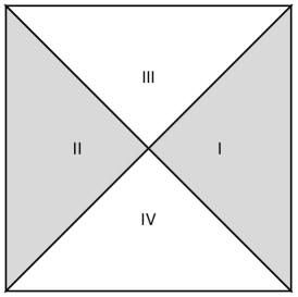
Figure 2: A Penrose diagram for de Sitter spacetime.

The modes we use in the static patch are normal modes found by Higuchi [29] which are also $\mathcal{L}^{2}$ orthogonal. Following the calculations of [30] we find in [19] that

$$A_{pp^{\prime}}=\frac{\delta(p-p^{\prime})}{1-e^{-2\pi p}},\;\;D_{pp^{\prime}}=\frac{\delta(p-p^{\prime})}{e^{2\pi p}-1}\;\;\text{and}\;\;B_{pp^{\prime}}=C_{pp^{\prime}}=0.$$ (3.25)

which then leads to the mode-wise contribution to SSEE

$$\mathcal{S}_{plm}=-\log(1-e^{-2\pi p})-\frac{e^{-2\pi p}}{1-e^{-2\pi p}}\log e^{-2\pi p},$$ (3.26)

which agrees with the von Neumann entropy evaluated by [30]. In particular, the result is independent of the mass.

In Schwarzschild de Sitter spacetime we compute the SSEE of a massless scalar field restricted to one of the static patches (region $I$ of Fig. 3)[19]. The field is assumed to be in the Kruskal vacuum state which is defined across the black hole horizon. We use static modes to expand the restriction of the Kruskal Wightman function to the static patch.

Figure 3: The Penrose diagram for the $d>2$ Schwarzschild de Sitter spacetime, where each point represents an $\mathbb{S}^{d-2}$ and each horizontal slice represents an $\mathbb{S}^{d-2}\times\mathbb{S}^{1}$. Region $I$ and $II$ are the static patches, and $\mathcal{H}_{b}^{\pm}$ and $\mathcal{H}_{c}^{\pm}$ are the black hole and the cosmological horizons respectively.

The massless scalar field modes (Kruskal and static) are not known in full static patch but since the SSEE depends only on the Bogoliubov transformation of these modes, the knowledge of the modes in a neighbourhood of a Cauchy hypersurface is sufficient to calulate the SSEE. We use the past boundary conditions for the static and the Kruskal modes, since this defines the Klein Gordon norm on the limiting initial null surface $\mathcal{H}_{b}^{-}\cup\mathcal{H}_{c}^{-}$ in Region I. As shown in [19] we find that

$$A_{pp^{\prime}}=\frac{\delta(p-p^{\prime})}{1-e^{-2\pi p/\kappa_{b}}},\quad D_{pp^{\prime}}=\frac{\delta(p-p^{\prime})}{e^{2\pi p/\kappa_{b}}-1},\;\;\text{and}\quad B_{pp^{\prime}}=C_{pp^{\prime}}=0.$$ (3.27)

which leads to the mode-wise contribution to SSEE

$$\mathcal{S}_{plm}=-\log(1-e^{-2\pi p/\kappa_{b}})-\frac{e^{-2\pi p/\kappa_{b}}}{1-e^{-2\pi p/\kappa_{b}}}\log e^{-2\pi p/\kappa_{b}}.$$ (3.28)

where $\kappa_{b}$ is the surface gravity of the black hole horizon.

We now move on to the next example which is the SSEE for a massless scalar field in a causal diamond inside a slab of 2d cylinder spacetime

$$ds^{2}=-dt^{2}+d\phi^{2},\quad\phi\sim\phi+2\pi.$$ (3.29)

We begin with the Fewster-Verch SJ vacuum $W_{\text{SJ}}$ in a slab of $t\in[-T,T]$ and restrict it to a causal diamond $\mathbb{D}_{2}$ as shown in Fig 4.

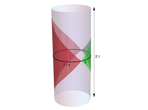
Figure 4: The causal diamond and its causal complement in the $d=2$ cylinder spacetime.

Let $L$ denote the circumference of the cylinder and $\ell$ the proper time of the causal diamond. Unlike the cases we have just studied, the restricted SJ Wightman function is not block diagonal with respect to the SJ modes in the diamond. Hence the analysis discussed above cannot be extended to get the generalised eigenvalues of the form given by Eqn. (3.14). Instead, as shown in [18] we use a combination of analytical and numerical techniques to calculate the generalised spectrum.

$\widehat{W}\big{|}_{\mathbb{D}_{2}}$ can be expanded in the SJ basis or eigenbasis of $i\widehat{\Delta}$ in diamond, but in general this expression does not have a closed form. Solving the generalised eigenvalue equation numerically therefore requires an additional cut-off. In [18] it was noticed that when the $\gamma=2T/L$ is a half integer and the ratio $\alpha=\ell/L$ is rational then $\widehat{W}\big{|}_{\mathbb{D}_{2}}$ simplifies considerably into a closed form expression. We refer the reader to [18] for details. In this case, the SSEE can be calculated numerically by imposing a covariant UV cut-off in the SJ spectrum in $\mathbb{D}_{2}$ which renders the problem finite.

We plot the SSEE for different values of the parameters $\alpha,\gamma$ and the cut-off $n_{\mathrm{max}}$ and use the best fit to obtain SSEE, which is of the form

$$\mathcal{S}_{\text{cyl}}=\frac{c(\gamma)}{3}\log\left(\frac{l}{\pi\epsilon}\right)+f(\gamma)\log\left(\sin(\pi\alpha)\right)+c_{1}(\gamma),$$ (3.30)

where $\epsilon$ is the UV cut-off, which in terms of the cut-off in SJ spectrum is given by

$$\epsilon=\frac{l\alpha}{2\sqrt{2}\pi n_{\mathrm{max}}}=\frac{l(1-\alpha)}{2\sqrt{2}\pi n_{\mathrm{max}}^{\prime}},$$ (3.31)

where $n_{\mathrm{max}}$ is the cut-off in the SJ spectrum. It is shown numerically in [18] using best fit curves that $c(\gamma)=1$, $f(\gamma)$ converges to unity for large enough $\gamma$ as shown in Fig. 5, and therefore the SSEE in Eqn. (3.30) reduces to the exact Calabrese-Cardy form in this limit. It is also clear from Eqn. (3.30) that the SSEE for a complimentary pair of diamonds are equal. $c_{1}(\gamma)$, which is a non-universal term in the Calabrese-Cardy entropy formula, inreases with $\gamma$ logarithmically.

Despite its asymptotic behaviour it is interesting that the coefficient $f(\gamma)$ is not “universal”. Importantly the SJ vacuum in the slab itself changes with $\gamma$ and is a pure state in the infinite cylinder, though not its ground state. Thus, one can view the SSEE that we have calculated to be that for a family of pure states in the infinite cylinder rather than that of its vacuum.

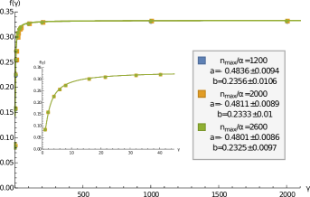
Figure 5: A plot of $f(\gamma)$ vs. $\gamma$ for different values of $n_{\mathrm{max}}/\alpha$, fitted to $0.33+a/\gamma+b/\gamma^{2}$. The inset figure shows the smaller $\gamma$ values.

4 SSEE in the Causal Set

Associated with every causal spacetime $(M,g)$, is a classical ensemble of causal sets $\{C\}$, where each $C$ is obtained via a Poisson sprinkling at density $\rho$ into $(M,g)$, with the order relations given by the continuum causality relations. For such a random discretisation, the probability of finding $n$ elements in a spacetime region $V$ is

$$P_{V}(n)=\frac{(\rho V)^{n}}{n!}e^{-\rho V}$$ (4.1)

and we have a mean number to volume correspondence

$$\langle N\rangle=\rho V.$$ (4.2)

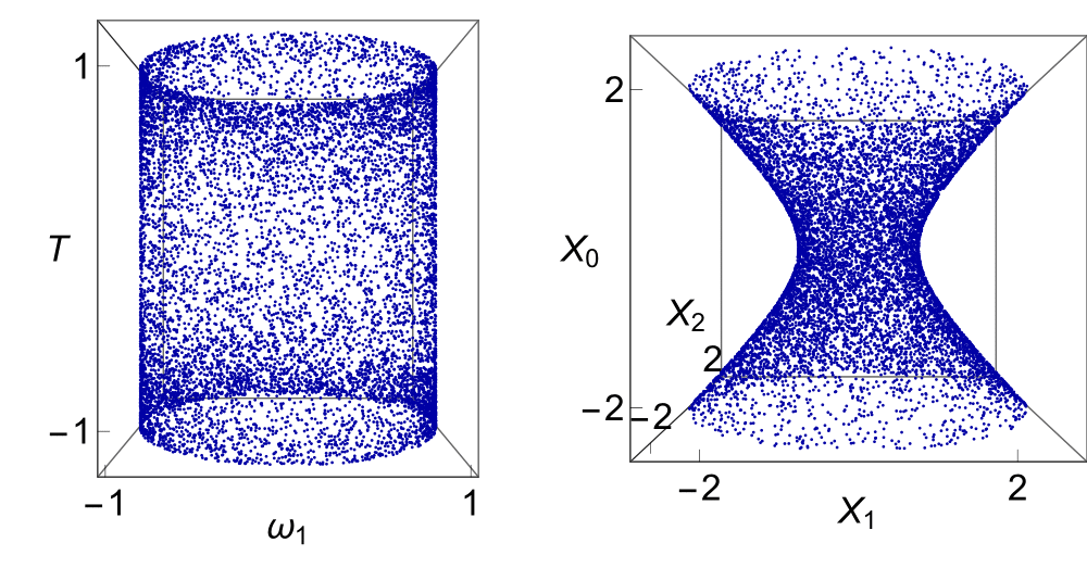
Figure 6: A causal set approximated by de Sitter spacetime. The representation on the left is in conformal coordinates and on the right is in usual hyperbolic coordinates.

Fig 6 is an example of a causal set that is approximated by de Sitter spacetime. Because of this discrete Poisson randomness, the causal set discretisation is covariant and locally Lorentz invariant, thus making it an ideal candidate for regulating the infinities of quantum field theory.

As before we concern ourselves only with the free scalar field theory, and construct the quantum vacuum via the Sorkin-Johnston procedure, which requires us to first obtain the advanced and retarded Green’s functions on $C$. We will need to define first the causal matrix

$$C_{0}(x,x^{\prime})\equiv\left\{\begin{array}[]{ll}1&\mbox{if }x^{\prime}\prec x\\ 0&\mbox{}\mathrm{otherwise}\end{array}\right.$$ (4.3)

and the link matrix

$$L_{0}(x,x^{\prime})\equiv\left\{\begin{array}[]{ll}1&\mbox{if }x^{\prime}\prec x\,\,\mathrm{and}\,\,|[x,x^{\prime}]|=0\\ 0&\mbox{}\mathrm{otherwise}\end{array}\right.$$ (4.4)

where $[x,x^{\prime}]\equiv\{z\in C\,|\,x^{\prime}\prec z\prec x\}$. The $k$-chain matrix is then $C_{k}\equiv C_{0}^{k}$ and the $k$-link matrix is then $L_{k}\equiv L_{0}^{k}$. As shown in [10], by comparing with the continuum in $\mathbb{M}^{2}$ and $\mathbb{M}^{4}$, the massless causal set Green’s functions can be written in terms of these matrices

$$K^{(2)}_{0}(x,x^{\prime})\equiv\frac{1}{2}C_{0}(x,x^{\prime}),\quad K^{(4)}_{0}(x,x^{\prime})=\frac{1}{2\pi}\sqrt{\frac{\rho}{6}}L_{0}(x,x^{\prime}),$$ (4.5)

respectively, and their massive counterparts by

$$K^{(2)}_{m}(x,x^{\prime})=\sum\limits_{k=0}^{\infty}\biggl{(}-\frac{m^{2}}{\rho}\biggr{)}^{k}\biggl{(}\frac{1}{2}\biggr{)}^{k+1}C_{k}(x,x^{\prime}),$$ (4.6)

and

$$K^{(4)}_{m}(x,x^{\prime})\equiv\sum\limits_{k=0}^{\infty}\biggl{(}-\frac{m^{2}}{\rho}\biggr{)}^{k}\biggl{(}\frac{1}{2\pi}\sqrt{\frac{\rho}{6}}\biggr{)}^{k+1}L_{k}(x,x^{\prime}).$$ (4.7)

respectively. In [31] it was shown that this simple form of the causal set Green’s function is still valid in the Riemann normal neighbourhoods of all $d=2$ spacetimes and those of $d=4$ spacetimes with $R_{ab}\propto g_{ab}$. Of relevance to this work is the result of [31] that this is also the Green’s function for $d=2$ and $d=4$ de Sitter and anti de Sitter spacetimes.

Using the Sorkin-Johnston formulation described in Section 2, one can then construct the scalar quantum field vacuum on causal sets approximated by this above set of of spacetimes. This is the starting point for finding the SSEE on causal sets.

As in the continuum, we are interested in finding the quantum scalar field SSEE in a causally convex subcausal set $C^{\prime}\subset C$ with respect to its causal complement. Starting with the SJ vacuum $\widehat{W}$ in $C$ which is a pure state, we wish to find the SSEE for the mixed state $\widehat{W}_{\mathcal{C}_{\mathcal{O}}}$ obtained by simply restricting to the region $C^{\prime}$.

The causal set SSEE mimics the one in the continuum with the added simplicity that operators and functions are realized as matrices, so that

$$\sum_{e^{\prime}\in C^{\prime}}W_{ee^{\prime}}\Psi_{e^{\prime}}=i\mu\sum_{e^{\prime}\in C^{\prime}}\Delta_{ee^{\prime}}\Psi_{e^{\prime}},\quad\Psi\not\in\mathrm{ker}\,{i\Delta},\quad\mathcal{S}=\sum_{\mu}\mu\ln|\mu|.$$ (4.8)

Because of the finiteness of the matrix it is already obvious that the SSEE is finite. In Fig 7 we show the behaviour of the SSEE for different manifold-like causal sets. What is obvious from all of these is that rather than an area law, the SSEE explicitly follows a volume law [20, 21].

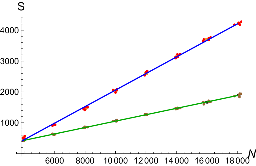
(a) causal diamonds in $\mathbb{M}^{4}$

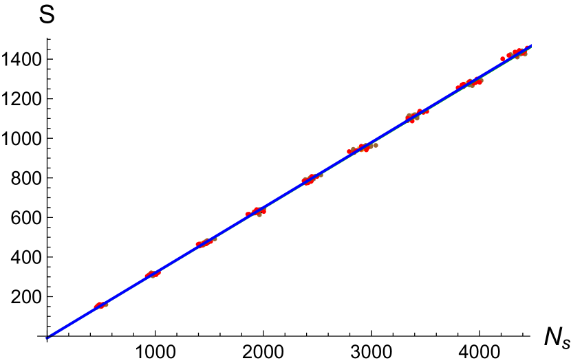
(b) $d=2$ de Sitter

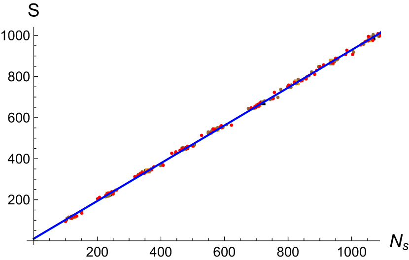
(c) $d=4$ de Sitter

Figure 7: SSEE vs. $N$ for the horizon EE of a causal set approximated by different spacetime regions. Green and blue represent the data for the two complemetary regions. Note that the complemetarity in the $\mathbb{M}^{4}$ case is not obvious because, unlike the de Sitter case, the volumes and geometry of the complementary regions are not the same.

There are two ways to interpret this result : (i) that the SSEE on causal sets is not a good measure of entanglement and should be modified somehow by inserting an additional cut-off or truncation in the spectrum because the quantum field theory in the deep UV cannot be trusted or (ii) that volume laws are natural for non-local field theories and since causal sets are fundamentally non-local, it is to be expected that one should get a volume law.

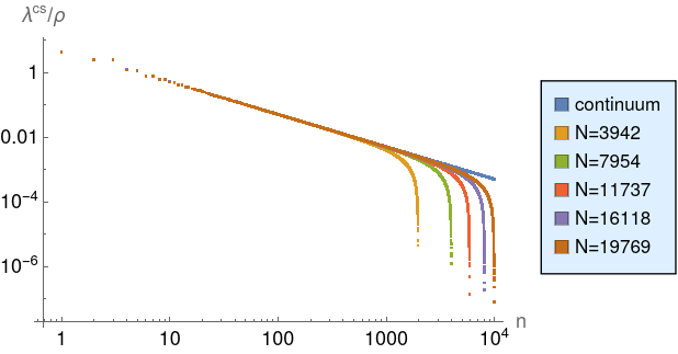
(a) $d=2$ de Sitter

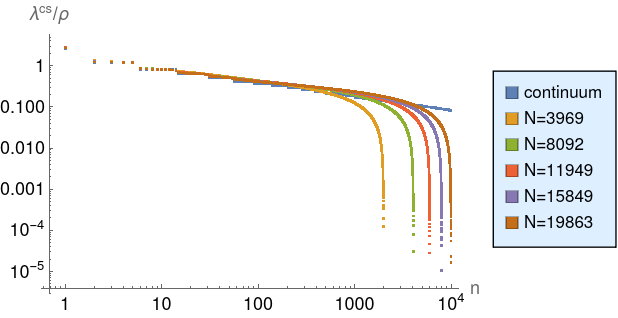
(b) $d=4$ de Sitter

Figure 8: A log-log plot of the SJ spectrum wavelength $\lambda$ versus quantum number $n$. The continuum spectrum shown in blue exhibits a scaling behaviour while the coloured plots are the causal set spectrum for different discreteness scales.

In the remaining part of this section we explore the first of these options and leave the second to the discussions section. The former gives us a way out of a volume law, by mimicking the UV cut-off required in the continuum. For this, it is instructive to examine Fig 1 where the SJ spectrum in a continuum $d=2$ causal diamond is plotted alongside that in the causal set at different sprinkling densities. Fig 8 shows a similar plot for de Sitter spacetime. The continuum spectrum in both cases follows a scaling behaviour

$$\lambda=\frac{b}{n^{\alpha}}$$ (4.9)

for some $\alpha$. The corresponding causal set spectrum $\rho^{-1}\lambda^{cs}$ on the other hand trails the scaling behaviour upto a “knee” beyond which its UV behaviour follows a wholly different, non-scaling form. Instead, a strong linear behaviour begins to dominate at large $n$ as shown in Fig. 9, so that we may write

$$\lambda^{cs}\sim\begin{cases}\dfrac{\beta_{1}}{n^{\alpha_{1}}},\quad n<n_{0}\\ \-\alpha_{2}n+\beta_{2},\quad n>n_{0}.\end{cases}$$ (4.10)

In the log-log plots of Fig  10, the full spectrum is shown to be roughly well modeled by a sum of these functions. An important qualitative feature of the spectrum is that even for large $n$ or the deep UV, far being random or chaotic, it is relatively smooth, rapidly approaching zero, as it should in any finite theory.

(a) Causal diamond in $\mathbb{M}^{2}$

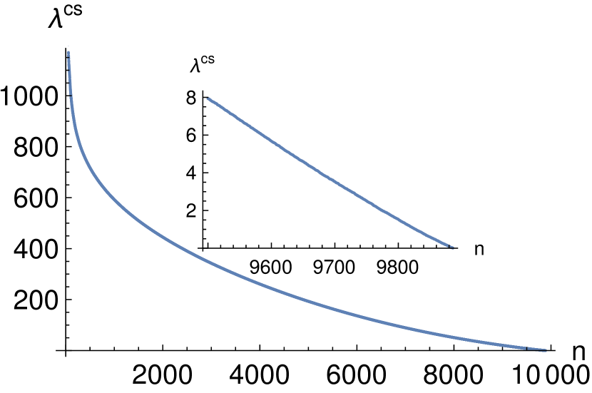
(b) Causal diamond in $\mathbb{M}^{4}$

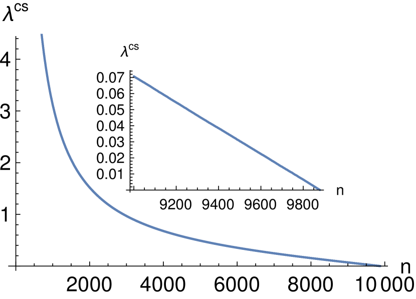
(c) $d=2$ de Sitter slab spacetime

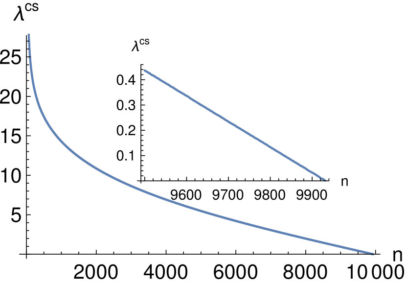
(d) $d=4$ de Sitter slab spacetime

Figure 9: The spectrum of $i\widehat{\Delta}$ for massless scalar field. For large $n$ the spectrum varies linearly with $n$ as shown in the inset figures. The continuum spectrum on the other hand follows a power law $\propto n^{-\alpha}$ with an infinitely long tail.

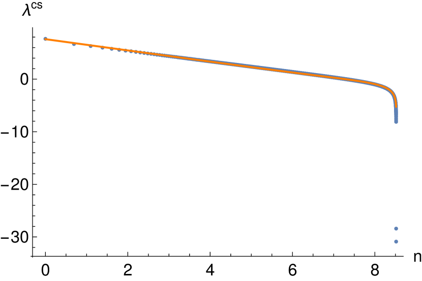
(a) Causal diamond in $\mathbb{M}^{2}$

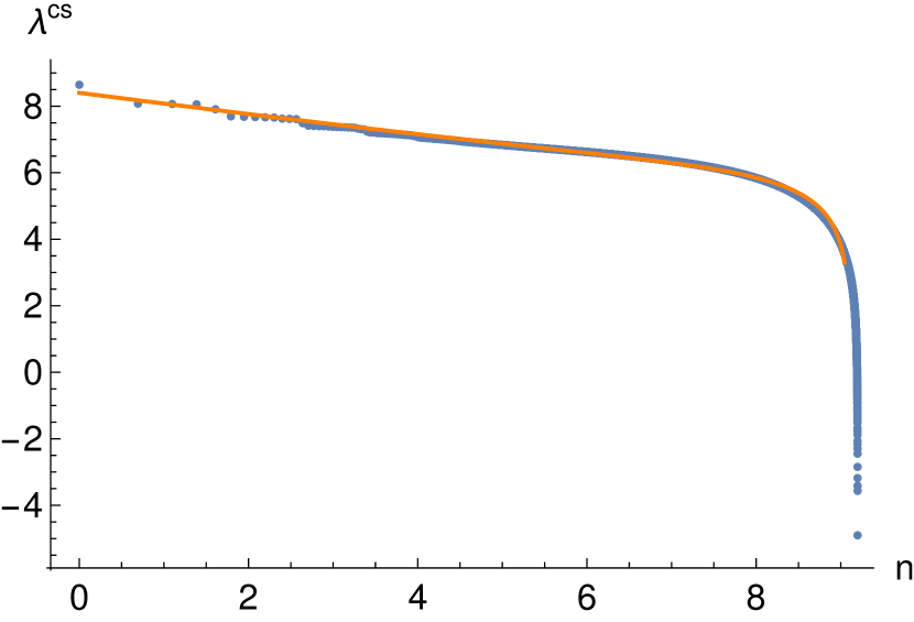
(b) Causal diamond in $\mathbb{M}^{4}$

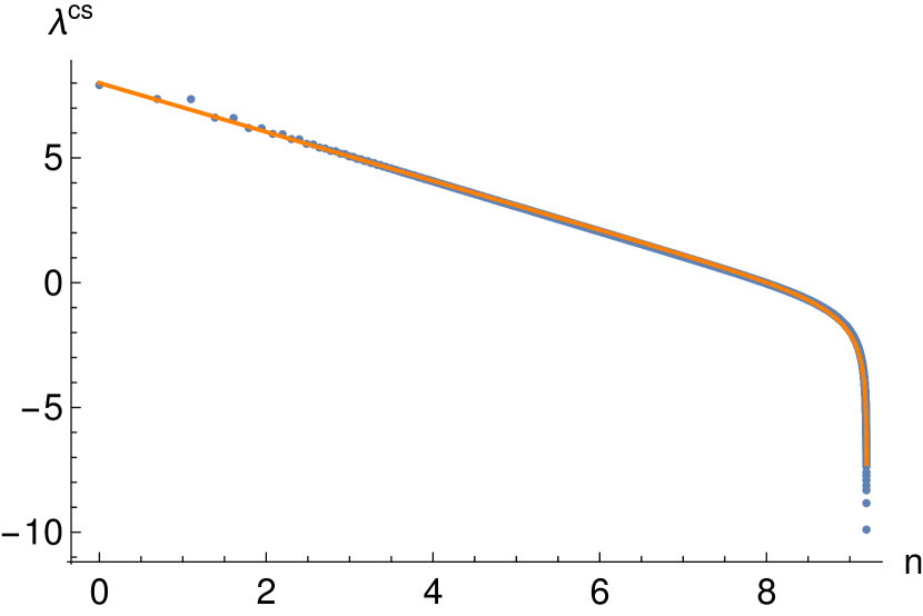
(c) $d=2$ de Sitter slab spacetime

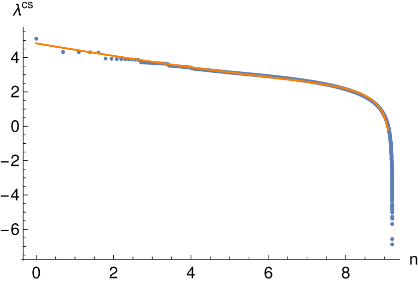
(d) $d=4$ de Sitter slab spacetime

Figure 10: A log-log plot of the spectrum of $i\widehat{\Delta}$ for massless scalar field. It follows $\lambda^{cs}=\dfrac{\beta_{1}}{n^{\alpha_{1}}}+\alpha_{2}n+\beta_{2}$ as shown in orange.

Beyond this knee, the spectrum consists of a large number of small but non-zero eigenvalues which dominate the SSEE.

In [20] the SSEE was recalculated in the $d=2$ nested causal set diamonds by employing a truncation of the causal set spectrum at the “knee”. Since this is at one end of the continuum-like scaling regime of the spectrum, it mimics the UV cut-off in the continuum SJ spectrum. However, it was shown in [20] that this is not in itself enough – one has to do a “double truncation” by truncating the SJ spectrum in the larger diamond and then truncating the SJ spectrum once again in the smaller diamond. This removes the additional high energy modes that creep back in after the first truncation.

In the causal diamond, the knee in the causal set SJ spectrum can be found simply by comparison with the continuum eigenvalues $\lambda=L/k$, where $2\sqrt{2}L$ is the proper time of the diamond and where $k\sim\dfrac{n\pi}{L}$ for large $k$. Causal set discreteness determines a “smallest wavelength” $\nu_{\text{min}}\sim\rho^{-1/2}=2L/\sqrt{N}=2\pi/k_{\text{max}}=2L/n_{\text{max}}$ or $n_{\text{max}}=\sqrt{N}$. Thus, a reasonable cut-off is $\lambda^{\text{cs}}_{\text{min}}=\rho\lambda_{\text{min}}=\sqrt{N}/4\pi$. In Fig 1 this value corresponds roughly to the knee of the causal set SJ spectrum.

In the absence of knowledge of the continuum spectrum, $n_{\text{max}}$ needs to be obtained from more general arguments. In the continuum, we expect the Cauchy hypersurface to contain all information about the QFT. Even though the dimension of $i\widehat{\Delta}$ is $N$, we know that the space of independent solutions of the equations of motion is spanned by $\mathrm{Image}(i\widehat{\Delta})$ [32] and that this picture should be consistent with the continuum. Therefore the dimension of $\mathrm{Image}(i\widehat{\Delta})$ must be related to the spatial volume of the Cauchy hypersurface which, for the symmetric slice at $t=0$ is $\sim\sqrt{N}$. This argument can be generalized (up to a proportionality constant) to other geometries without knowing the functional form of the eigenvalues.

$$n_{\mathrm{max}}=\mathrm{\alpha}{N}^{\frac{d-1}{d}}.$$ (4.11)

In general, the Cauchy hypersurface can be deformed to minimize the spatial volume. Therefore, the choice of $\alpha$ is neither unique nor covariant. In the examples below, we will see that the choice of this parameter is non-trivial and is based on the coefficients we expect in the area law and on requiring complementarity.

Another possible truncation scheme, called “linear truncation” has been used. It is based on numerically identifying the location of the knee in the spectrum. This involves comparison of the slopes and detection of a rapid fall in the slopes in the spectrum. Again, the choice of what ‘rapid’ means is captured by a single parameter $\delta$ and this choice is dictated by various factors as mentioned above. The advantage of this method is that it is independent of the geometry or any other detail about the QFT. The details of this scheme can be found in [21].

Before proceeding we must ask what an area law looks like on a causal set. Since the areas in question are of co-dimension $2$ surfaces, these are sets of measure zero in the causal set discretisation. On the other hand, given that there is a length scale $\rho^{-1/d}$ associated with the discreteness scale, one can ascribe to the causal set a dimension dependent scale $N^{-1/d}$. Thus, we expect that an area law for $d>2$ should to be of the form

$$S^{cs}_{d}=aN^{\frac{d-2}{d}}+b.$$ (4.12)

For $d=2$ in the continuum the EE satisfies the log behaviour [33]

$$\mathcal{S}=\frac{1}{3}\log\bigg{(}\frac{l}{\epsilon}\bigg{)}+b,$$ (4.13)

where $\epsilon$ is the cut-off. Thus, in the causal set we expect that

$$S^{cs}_{2}=a\ln N+b$$ (4.14)

The truncation procedure employed in [20] for the nested causal diamonds in $\mathbb{M}^{2}$ and adapted to nested causal diamonds in $\mathbb{M}^{4}$ as well as $d=2,4$ de Sitter horizons can be summarised as below.

$$\begin{array}[]{ccccc}i\widehat{\Delta}&\text{truncation}&i\widehat{\Delta}^{\text{t}}&\stackrel{{\scriptstyle SJ}}{{\Rightarrow}}&\widehat{W}^{\text{t}}\\ &&\big{\downarrow}&\text{restriction}&\big{\downarrow}\\ &&i\widehat{\Delta}_{\mathcal{O}}^{\text{t}}&&\widehat{W}^{\text{t}}_{\mathcal{O}}\\ &&\big{\downarrow}&\text{truncation}&\big{\downarrow}\\ &&i\widehat{\Delta}^{\text{t}\text{t}}_{\mathcal{O}}&&\widehat{W}^{\text{tt}}_{\mathcal{O}}.\end{array}$$ (4.15)

One starts with the Pauli Jordan operator $i\widehat{\Delta}$ in $C$. Its spectrum is then truncated to obtain $i\widehat{\Delta}^{\text{t}}$ and this gives a truncated SJ Wightman function $\widehat{W}^{\text{t}}$. The restriction of $\widehat{W}^{\text{t}}|_{\mathcal{O}}$ to the subcausal set $\mathcal{O}$ is however is not truncated with respect to the spectrum of $i\widehat{\Delta}$ in $\mathcal{O}$. Hence there is need for a second truncation of the SJ spectrum of $i\widehat{\Delta}$ in $\mathcal{O}$ which removes the large discrete UV contributions. Thus, the double truncated $\widehat{W}^{\text{tt}}|_{\mathcal{O}}$ is used along with the truncated $i\widehat{\Delta}^{\text{t}}|_{\mathcal{O}}$ to solve the generalised SSEE eigenvalue function in $\mathcal{O}$.

Figure 11 summarises the results. What is remarkable is that this truncation does what is expected of it – it restores an area law. The case of the nested causal diamonds in $\mathbb{M}^{4}$ is however unsatisfying. The area law should come hand in hand with complementarity, but this does not seem to be the case for any of the choices of truncation. In the de Sitter case, we cannot check for complementarity since the de Sitter horizon is symmetric and the complementary regions are equivalent. However, here too an area law emerges for suitable truncation schemes.

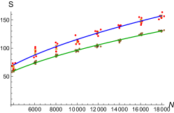
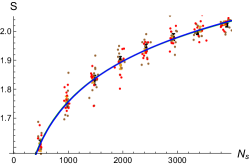
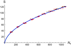
(a) Number truncation

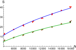
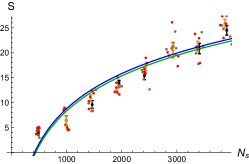
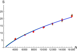
(b) Linear truncation

Figure 11: SSEE vs. $N$ for the EE of horizons in $\mathbb{M}^{4}$ and de Sitter in 2 and 4 dimensions with two different truncations. Green and blue represent the data for the complementary regions.

This double truncation in the SJ spectrum therefore has a profound effect on the generalised eigenvalue spectrum which defines the SSEE. In Fig 12 this effect is shown for the nested causal diamonds in $\mathbb{M}^{4}$. What is remarkable is that the truncation leads to much smaller eigenvalues and hence a much smaller SSEE. In contrast, the untruncated generalised spectrum contains very large eigenvalues.

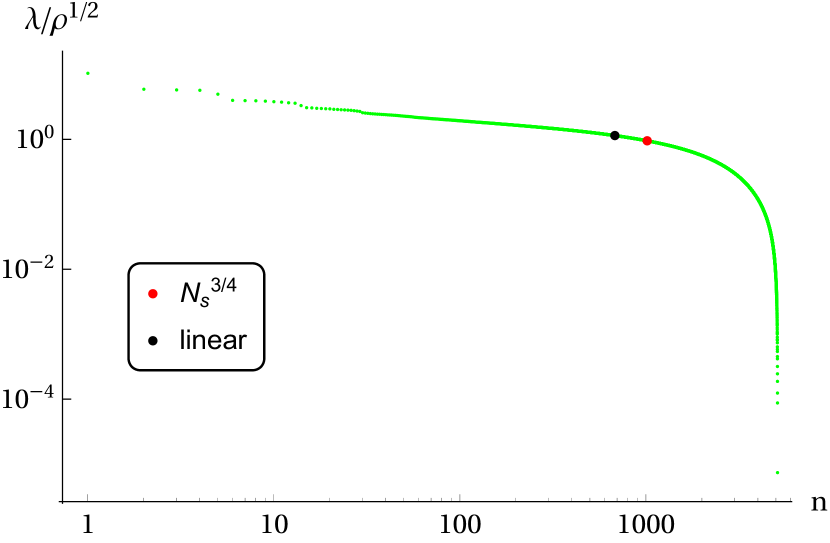
(a)

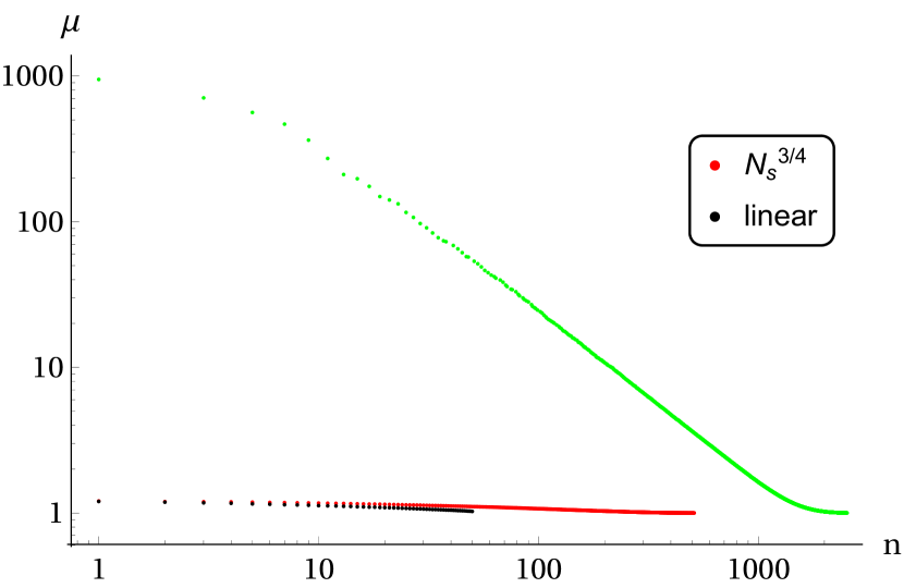
(b)

Figure 12: For a causal diamond in $\mathbb{M}^{4}$ with $N=10k$, (a) is the spectrum of $i\Delta$ with different truncations marked, and (b) is a plot of the solutions of the generalised SSEE equation for these truncation schemes.

5 Discussion

The foremost question that emerges is why the causal set SSEE has a volume dependence in the first place and how we should interpret the double truncation procedure since there should be no need for it in an already finite theory. By trying to obtain a continuum-like result the worry is that one may be unnecessarily throwing out an important sign of new UV physics.

As noted in [34] the double truncation procedure leads to small violations of causality. Namely, after the spectral truncation $\widehat{\Delta}\rightarrow\widehat{\Delta}^{\text{tt}}$, $\Delta^{\text{tt}}(e,e^{\prime})$ does not always vanish for spacelike pairs $(e,e^{\prime})$. These violations are “small” and become negligible when suitably averaged over the ensemble. Adding to this is the work of [27] where the SJ eigenfunctions in the $d=2$ causal diamond were examined in more detailed. They found that the eigenfunctions beyond the knee were highly fluctuating at and “below” the discreteness scale. They moreover vary considerably over the causal set ensemble unlike those in the scaling-regime which retain their general form. These results are an indication that truncation may be physically justified in a coarse grained, averaged sense, at length scales larger than the truncation length scale. Indeed, in [20, 35] it has been suggested that since the SJ spectrum beyond the knee contains modes with very small eigenvalues, which are “nearly” in $\ker\Delta$, the SSEE formula itself is not well defined. Such modes are indeed what dominate the SSEE in the absence of truncation and give rise to the volume law.

One conclusion is that we cannot really speak of the QFT UV regime without a full quantum theory of causal sets. Indeed, in all our discussions we have used only a classical causal set ensemble. It is plausible that the observables of the full theory are therefore such that one could still recovers an area law.

In the absence of such a full quantisation, however it is reasonable to look for the effects of causal set discreteness in a phenomenologically interesting regime of quantum field theory. Manifold-like causal sets become important when $\rho^{-1/d}$ is much larger than the Planck scale so that we can talk of the continuum approximation, while ignoring non-manifold-like contributions arising from full causal set quantum gravity [36, 37, 38, 39]. This interim “kinematic” regime, between known physics and the Planck scale can lead to interesting new physics as discussed in [40, 41]. It is in this regime that we place the above analysis of quantum field theory on causal sets. Rather than a “complete” quantum gravity theory of QFT we wish to look at the regime in which discreteness does play a role. Thus, far from being an artifact, the non-scaling UV behaviour of the spectrum and the resultant volume law for the SSEE could be a sign of new physics.

It has for example been suggested in [6] that the effects of non-locality in quantum gravity could lead to volume laws for entanglement entropy. If this were true, then we would need to understand the transition from a non-local (volume-law) regime to a local field theory (area-law) regime as one moves away from the deep UV. While the analysis on causal sets shows this explicitly with the causal set spectrum exhibiting a non-scaling behaviour in the deep UV, it is important to understand this transition better, possibly from an RG perspective.

An interesting question is whether there is a physical process which realises this transition to the deep UV. Roughly, one might expect that “entanglement probes” with energies in the scaling regime would conclude that there is an area law, but those that are more energetic, would uncover a volume law. This suggests a kind of “screening” of the interior of horizons for intermediate energy probes which gives rise to an effective area law, whereas the horizon interiors are entangled with very high energy probes. Constructing an appropriate probe in the causal set quantum field theory is of course a challenge. Given the emerging work on volume laws in condensed matter systems it may be a fruitful first step to construct suitable analogues in random lattice-like systems.

Of course there is the bigger question of what a volume-law might mean for blackhole evaporation, but given that such systems are challenging to study in causal sets, we leave that as a question for the future.

Acknowledgements: We would like to thank Yasaman Yazdi and Maximillian Ruep for discussions. NX is supported by the AARMS fellowship at UNB.

Data sharing not applicable to this article as no datasets were generated or analysed during the current study.

References

- [1] L. Bombelli, R. K. Koul, J. Lee, and R. D. Sorkin, “A Quantum Source of Entropy for Black Holes,” Phys. Rev., vol. D34, pp. 373–383, 1986.
- [2] S. Ryu and T. Takayanagi, “Holographic derivation of entanglement entropy from AdS/CFT,” Phys. Rev. Lett., vol. 96, p. 181602, 2006.
- [3] D. Vodola, L. Lepori, E. Ercolessi, and G. Pupillo, “Long-range ising and kitaev models: phases, correlations and edge modes,” New Journal of Physics, vol. 18, no. 1, p. 015001, 2015.
- [4] J. L. Karczmarek and P. Sabella-Garnier, “Entanglement entropy on the fuzzy sphere,” Journal of High Energy Physics, vol. 2014, no. 3, 2014.
- [5] N. Shiba and T. Takayanagi, “Volume law for the entanglement entropy in non-local QFTs,” Journal of High Energy Physics, vol. 2014, no. 2, 2014.
- [6] B. Basa, G. La Nave, and P. W. Phillips, “Classification of nonlocal actions: Area versus volume entanglement entropy,” Phys. Rev. D, vol. 101, no. 10, p. 106006, 2020.
- [7] Y. O. Nakagawa, M. Watanabe, H. Fujita, and S. Sugiura, “Universality in volume-law entanglement of scrambled pure quantum states,” Nature Communications, vol. 9, no. 1, 2018.
- [8] L. Bombelli, J. Lee, D. Meyer, and R. Sorkin, “Space-Time as a Causal Set,” Phys. Rev. Lett., vol. 59, pp. 521–524, 1987.
- [9] S. Surya, “The causal set approach to quantum gravity,” Living Rev. Rel., vol. 22, no. 1, p. 5, 2019.
- [10] S. Johnston, “Particle propagators on discrete spacetime,” Class. Quant. Grav., vol. 25, p. 202001, 2008.
- [11] S. Johnston, “Feynman Propagator for a Free Scalar Field on a Causal Set,” Phys. Rev. Lett., vol. 103, p. 180401, 2009.
- [12] S. P. Johnston, Quantum Fields on Causal Sets. PhD thesis, Imperial Coll., London, 2010.
- [13] R. D. Sorkin, “Scalar Field Theory on a Causal Set in Histories Form,” J. Phys. Conf. Ser., vol. 306, p. 012017, 2011.
- [14] C. J. Fewster and R. Verch, “On a Recent Construction of ’Vacuum-like’ Quantum Field States in Curved Spacetime,” Class. Quant. Grav., vol. 29, p. 205017, 2012.
- [15] M. Brum and K. Fredenhagen, “‘Vacuum-like’ Hadamard states for quantum fields on curved spacetimes,” Class. Quant. Grav., vol. 31, p. 025024, 2014.
- [16] R. D. Sorkin, “Expressing entropy globally in terms of (4D) field-correlations,” J. Phys. Conf. Ser., vol. 484, p. 012004, 2014.
- [17] M. Saravani, R. D. Sorkin, and Y. K. Yazdi, “Spacetime entanglement entropy in 1+ 1 dimensions,” Classical and Quantum Gravity, vol. 31, no. 21, p. 214006, 2014.
- [18] A. Mathur, S. Surya, and Nomaan X, “A spacetime calculation of the Calabrese-Cardy entanglement entropy,” Phys. Lett. B, vol. 820, p. 136567, 2021.
- [19] A. Mathur, S. Surya, and Nomaan X, “Spacetime entanglement entropy of de Sitter and black hole horizons,” Class. Quant. Grav., vol. 39, no. 3, p. 035004, 2022.
- [20] R. D. Sorkin and Y. K. Yazdi, “Entanglement Entropy in Causal Set Theory,” Class. Quant. Grav., vol. 35, no. 7, p. 074004, 2018.
- [21] S. Surya, Nomaan X, and Y. K. Yazdi, “Entanglement entropy of causal set de sitter horizons,” Classical and Quantum Gravity, vol. 38, p. 115001, apr 2021.
- [22] N. Afshordi, S. Aslanbeigi, and R. D. Sorkin, “A Distinguished Vacuum State for a Quantum Field in a Curved Spacetime: Formalism, Features, and Cosmology,” JHEP, vol. 08, p. 137, 2012.
- [23] S. Aslanbeigi and M. Buck, “A preferred ground state for the scalar field in de Sitter space,” JHEP, vol. 08, p. 039, 2013.
- [24] N. Afshordi, M. Buck, F. Dowker, D. Rideout, R. D. Sorkin, and Y. K. Yazdi, “A Ground State for the Causal Diamond in 2 Dimensions,” JHEP, vol. 10, p. 088, 2012.
- [25] S. Surya, Nomaan X, and Y. K. Yazdi, “Studies on the SJ Vacuum in de Sitter Spacetime,” JHEP, vol. 07, p. 009, 2019.
- [26] Y. Chen, L. Hackl, R. Kunjwal, H. Moradi, Y. K. Yazdi, and M. Zilhão, “Towards spacetime entanglement entropy for interacting theories,” JHEP, vol. 11, p. 114, 2020.
- [27] T. Keseman, H. J. Muneesamy, and Y. K. Yazdi, “Insights on Entanglement Entropy in Dimensional Causal Sets.” arXiv:2111.05879 (2021), 11 2021.
- [28] T. Bunch and P. Davies, “Quantum Field Theory in de Sitter Space: Renormalization by Point Splitting,” Proc. Roy. Soc. Lond. A, vol. A360, pp. 117–134, 1978.
- [29] A. Higuchi, “Quantization of Scalar and Vector Fields Inside the Cosmological Event Horizon and Its Application to Hawking Effect,” Class. Quant. Grav., vol. 4, p. 721, 1987.
- [30] A. Higuchi and K. Yamamoto, “Vacuum state in de Sitter spacetime with static charts,” Phys. Rev. D, vol. 98, no. 6, p. 065014, 2018.
- [31] Nomaan X, F. Dowker, and S. Surya, “Scalar Field Green Functions on Causal Sets,” Class. Quant. Grav., vol. 34, no. 12, p. 124002, 2017.
- [32] R. M. Wald, Quantum Field Theory in Curved Spacetime and Black Hole Thermodynamics. Chicago, USA: Chicago Univ. Pr., 1994.
- [33] P. Calabrese and J. L. Cardy, “Entanglement entropy and quantum field theory,” J. Stat. Mech., vol. 0406, p. P06002, 2004.
- [34] Nomaan X, Aspects of Quantum Fields on Causal Sets. PhD thesis, Jawaharlal Nehru University, 5 2021.
- [35] A. Belenchia, D. M. T. Benincasa, M. Letizia, and S. Liberati, “On the Entanglement Entropy of Quantum Fields in Causal Sets,” Class. Quant. Grav., vol. 35, no. 7, p. 074002, 2018.
- [36] D. J. Kleitman and B. L. Rothschild, “Asymptotic enumeration of partial orders on a finite set,” Trans. Amer. Math. Soc., vol. 205, pp. 205–220, 1975.
- [37] S. Loomis and S. Carlip, “Suppression of non-manifold-like sets in the causal set path integral,” Class. Quant. Grav., vol. 35, no. 2, p. 024002, 2018.
- [38] A. Mathur, A. A. Singh, and S. Surya, “Entropy and the Link Action in the Causal Set Path-Sum,” Class. Quant. Grav., vol. 38, no. 4, p. 045017, 2021.
- [39] P. Carlip, S. Carlip, and S. Surya.
- [40] M. Ahmed, S. Dodelson, P. B. Greene, and R. Sorkin, “Everpresent ,” Phys. Rev. D, vol. 69, p. 103523, 2004.
- [41] F. Dowker, J. Henson, and R. D. Sorkin, “Quantum gravity phenomenology, lorentz invariance and discreteness,” Modern Physics Letters A, vol. 19, no. 24, pp. 1829–1840, 2004.