Synthesis of General Decoupling Networks Using Transmission Lines

Abstract

In this paper, we introduce a synthesis technique for transmission line based decoupling networks, which find application in coupled systems such as multiple-antenna systems and antenna arrays. Employing the generalized $\pi$-network and the transmission line analysis technique, we reduce the decoupling network design into simple matrix calculations. The synthesized decoupling network is essentially a generalized $\pi$-network with transmission lines at all branches. The advantage of this proposed decoupling network is that it can be implemented using transmission lines, ensuring better control on loss, performance consistency and higher power handling capability, when compared with lumped components, and can be easily scaled for operation at different frequencies.

I Introduction

Antenna arrays and multiple-antenna systems typically suffer from mutual coupling effect, which causes lower system efficiency, impedance mis-matching [1] and correlation-induced capacity reduction [2]. Therefore, a decoupling network that combats the mutual coupling effect is of great interest to such coupled systems. The reported works in literature on decoupling techniques typically deal with coupled networks with special characteristics, such as circular symmetry [3], and systems with limited number of ports [4]. To the best of the author’s knowledge, the first few general decoupling networks are reported in [5], [6] and [7]. In [5], a decoupling network using lumped elements is proposed based on the analysis of generalized LC $\pi$-network. However, its implementation using lumped elements suffers from parasitic effects and losses in lumped elements. Moreover, in real application, extra physical layout traces are needed and will add extra transmission line effects to it, potentially deviating the performance from the synthesized optimal case, especially at high frequencies. In [6], multi-port decoupling networks are synthesized using directional couplers, and are again implemented using lumped components. In [7], a decoupling network using transformer banks is proposed, which uses the minimum number of components for general decoupling and matching, and whose implementation requires efficient transformers at radio and microwave frequency ranges.

In [8], a network synthesis technique using transmission lines is proposed. Though generic, the paper [8] fails to propose a network topology that could synthesize arbitrary networks, and only conventional ring hybrid and directional couplers are considered in the given examples. Moreover, the solution approach depending entirely on ABCD parameters makes it cumbersome for different systems with different number of ports, as new equations has to be derived once the number of ports are changed.

In this paper, we will demonstrate that a TL-based generalized $\pi$-network can be used to synthesize an arbitrary passive, reciprocal and lossless decoupling network, and the analysis of the proposed network is based on Y parameters, and as will be seen significantly simplifies the analysis. The same set of equations can be scaled to analyze networks with arbitrary number of ports.

II Theory of the TL-based Decoupling Network

The proposed DN is based on a generalized $\pi$-network of transmission lines as shown in Fig. 1 for a two-port antenna system. For an N-port coupled system, the DN will be a 2N port network. Each branch of the network represents a transmission line. For a uniform transmission line with the characteristic impedance $Z_{0}$ and the electrical length $\theta$, we can parameterize it using ABCD parameters as

$$A_{TL}=\begin{bmatrix}\cos\theta&jZ_{0}\sin\theta\\ jY_{0}\sin\theta&\cos\theta\end{bmatrix}=\begin{bmatrix}a&jb\\ jc&a\end{bmatrix},$$ (1)

where $a=\cos\theta$, $b=Z_{0}\sin\theta$, and $a^{2}+bc=1$.

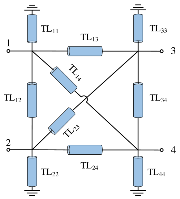
Figure 1: The topology of the generalized TL $\pi$ network (two-port case)

The admittance Y parameter of one TL branch can then be represented as [9]

$$Y_{TL}=\begin{bmatrix}\frac{a}{jb}&\frac{-1}{jb}\\ \frac{-1}{jb}&\frac{a}{jb}\end{bmatrix}$$ (2)

Following the analysis in [5], the Y parameter of a 2N-port generalized $\pi$-network can be assembled from the Y parameters of each branch as

$$Y_{\Pi}=\begin{bmatrix}\sum_{k=1}^{2N}\frac{a_{1,k}}{jb_{1,k}}&\frac{-1}{jb_{1,2}}&\frac{-1}{jb_{1,3}}&\dots&\frac{-1}{jb_{1,2N}}\\ \frac{-1}{jb_{2,1}}&\sum_{k=1}^{2N}\frac{a_{2,k}}{jb_{2,k}}&\frac{-1}{jb_{2,3}}&\dots&\frac{-1}{jb_{2,2N}}\\ \frac{-1}{jb_{3,1}}&\frac{-1}{jb_{3,2}}&\sum_{k=1}^{2N}\frac{a_{3,k}}{jb_{3,k}}&\dots&\frac{-1}{jb_{3,2N}}\\ \vdots&\vdots&\vdots&\ddots&\vdots\\ \frac{-1}{jb_{2N,1}}&\frac{-1}{jb_{2N,2}}&\frac{-1}{jb_{2N,3}}&\dots&\sum_{k=1}^{2N}\frac{a_{2N,k}}{jb_{2N,k}}\end{bmatrix}$$ (3)

where $b_{n,k}=b_{k,n}$ and $a_{n,k}=a_{k,n}$ due to reciprocity of the each transmission line branch.

In the proposed TL-decoupling network, the number of unknowns to be decided is $(4N^{2}+2N)$ (two unknowns $a$ and $b$, or $Z_{0}$ and $\theta$ for each branch), which is twice as many as what is needed to synthesize an arbitrary 2N-port network [5]. By enforcing the characteristic impedance (or the electrical length) on each branch, the number of unknowns is reduced to $2N^{2}+N$. By enforcing a conjugate matching with the $N-$port load, the number of unknowns is reduced to $N^{2}$. As discussed in [5], this $N^{2}$ design freedom implies that there is no unique solution for the DN, and can be leveraged to simplify the design topology or optimize the matching bandwidth.

II-A DN Synthesis Process

Before synthesizing the TL DN, a mathematical DN that achieves the decoupling is needed, which can be obtained using different methods [5, 10]. We here adopt the decoupling network in [5], which is based on the singular value decomposition of the load impedance $S_{L}=U_{L}^{H}\Lambda_{L}V_{L}$ with its S parameter given below:

$$S_{DN}=\begin{bmatrix}-VV_{L}^{\mathrm{H}}U_{L}^{*}\Lambda_{L}V^{T}&V(I-\Lambda_{L}^{2})^{\frac{1}{2}}U_{L}^{\mathrm{H}}\\ U_{L}^{*}(I-\Lambda_{L}^{2})^{\frac{1}{2}}V^{T}&V_{L}\Lambda_{L}U_{L}^{\mathrm{H}}\end{bmatrix}$$ (4)

As noted in [5], the unitary matrix $V$ is random, and represents the $N^{2}$ design freedom. Each unitary matrix $V$ corresponds to an $S_{DN}$. The decoupling network admittance matrix $Y_{DN}$ can be obtained through direct S to Y conversion.

For the TL DN synthesis, to ensure a TL implementation, we first specify all the $a$ in the transmission lines to be some value in the range of $-1$ and $1$, and then equate $Y_{\Pi}$ with the admittance of the to-be-synthesized $N-$port network $Y_{DN}$ to get the solution of the remaining unknowns (all the $b$’s).

With the values of $a$ and $b$ on each TL branch, we can convert that to the electrical length and characteristic impedance of the TL branch using the following relation

$$\theta=\cos^{-1}a$$ (5)

$$Z_{0}=b/\sin\theta$$ (6)

Though it is always desirable to have a small $\theta$ to make the TL shorter, sometimes the resulted $b$ being negative requires that $\sin\theta$ has to be negative. In this case, the $\theta$ derived from (5) has to be modified as $2\pi-\theta$ to meet the requirement.

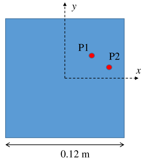
(a)

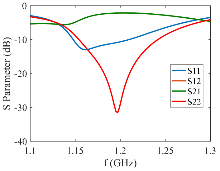
(b)

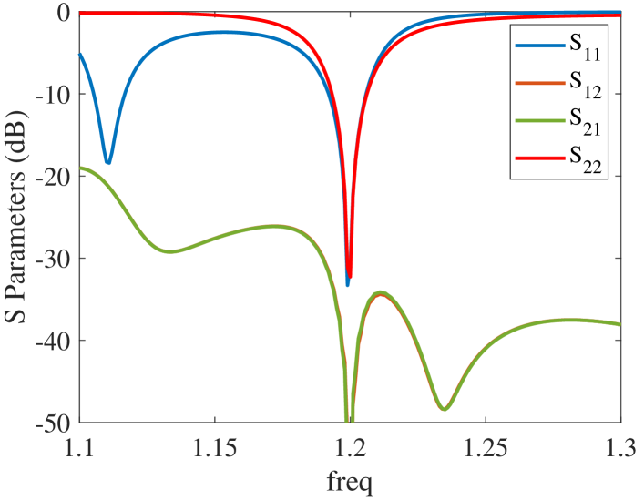
(c)

Figure 2: (a) the geometry of the two-port square patch antenna, (b) the original S parameter behavior of the two-port patch, (c) the S parameter of the two-port patch with DN synthesized using standard electrical length ($S_{12}$ overlaps with $S_{21}$).

II-B DN Synthesis with Standard Electrical Length

As stated above, the TL-based DN has double the number of unknowns compared with and LC DN network. To reduce the number of unknowns and standardize the DN implementation, we here fix certain parameters. Specifically, $\cos\theta$ is set as $-1/\sqrt{2}$, namely an electrical length of $3\lambda/8$ or $5\lambda/8$ long. The parameters we can freely choose are then characteristic impedance $Z_{0}$ for each branch TL. The resulting ABCD parameter of the TL section is

$$A_{TL}=\frac{-1}{\sqrt{2}}\begin{bmatrix}1&jZ_{0}\tan\theta\\ jY_{0}\tan\theta&1\end{bmatrix}$$ (7)

where $a=\frac{-1}{\sqrt{2}}$, and $b=-Z_{0}\tan\theta/\sqrt{2}$.

Following similar analysis as in Section II-A to determine the $b$ values (by matching the $Y_{\Pi}$ to the $Y_{DN}$), the length of each TL branch then be determined. In this case, the electrical length and the $Z_{0}$ of each TL branch depends on the $b$ value as

$$l=\begin{cases}3\lambda/8&\text{if $b>0$}\\ 5\lambda/8&\text{if $b<0$}\end{cases}$$ (8)

$$Z_{0}=\sqrt{2}|b|$$ (9)

It’s worth noting that the choice of $l$ could also be $\lambda/8$ and $7\lambda/8$ if $\cos\theta=1/\sqrt{2}$. We here select the relation in (9) in consideration of easier layout with comparable TL lengths.

III Design Examples

Two numerical examples are examined here to validate the proposed DN. To avoid randomness and facilitate crosscheck, we pick the $V$ in (4) as an identity matrix when determining our $S_{DN}$.

III-A Two-port System

The first example is a two-port patch antenna. As shown in Figure 2 (a), the square patch has two ports arbitrarily placed at P1 (0.025,0.021) and P2 (0.044,0.009). The patch has a size of $0.12\times 0.12$ m², and is placed 5 mm above the ground plane with an air substrate. The frequency response of the antenna before decoupling is shown in Figure 2 (b). Strong mutual coupling is clearly observed between the two ports.

Following the analysis in Section II, a DN based on generalized $\pi$ TL network is synthesized. Standard electrical length is used here for design simplification. Table I shows the corresponding electrical length and characteristic impedance of each TL branch for the DN. Figure 2 (c) shows the S parameter of the two-port antenna after inserting the synthesized TL-based DN. As expected, the two ports are decoupled at the design frequency.

TABLE I: Decoupling Network Parameters for the Two-Port System with Standard Electrical Length

TL Branch	$Z_{0}$ ($\Omega$)	$\theta$ (degree)
$TL_{11}$	109.71	225
$TL_{12}$	15425.54	225
$TL_{13}$	196.00	135
$TL_{14}$	239.55	225
$TL_{22}$	88.71	135
$TL_{23}$	127.90	135
$TL_{24}$	100.43	135
$TL_{33}$	42.35	135
$TL_{34}$	69.50	225
$TL_{44}$	43.51	135

III-B Three-port System

Here a three-port antenna system based on strongly coupled monopoles operating at 1 GHz is used for the DN test. As shown in Figure 3 (a), the monopoles are quarter wavelength long, 1mm in radius, and are placed asymmetrically. Antennas 1 and 2 are quarter-wavelength spaced, and antennas 1 and 3 are sixth-wavelength spaced. Antenna 2 and 3 are placed at a right angle from antenna 1. The response of the three-port antenna is shown in Figure 3 (b), where mutual couplings around -10 dB are observed.

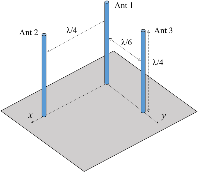
(a)

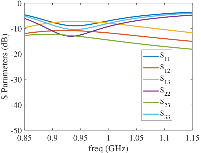
(b)

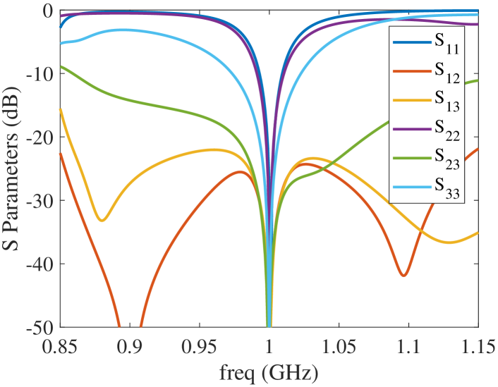
(c)

Figure 3: (a) the geometry of the three monopoles, (b) the original S parameter behavior of the three monopoles, (c) the S parameter of the three monopoles with DN synthesized using standard electrical length.

A DN using the standard electrical length is synthesized based on the method discussed in Section II. The resulted TL-DN parameters are given in Table II. Ports 1, 2, 3 corresponds to the decoupled ports, and ports 4, 5, 6 corresponds to the antenna ports. The decoupled three-port response is shown in Figure 3 (c). Again, all three ports are decoupled at the operation frequency.

TABLE II: Decoupling Network Parameters for the Three-Port System with Standard Electrical Length

TL Branch	$Z_{0}$ ($\Omega$)	$\theta$ (degree)
$TL_{11}$	65.75	225
$TL_{12}$	3492.69	135
$TL_{13}$	679.90	135
$TL_{14}$	141.82	225
$TL_{15}$	371.42	135
$TL_{16}$	168.33	135
$TL_{22}$	31.79	225
$TL_{23}$	164.19	225
$TL_{24}$	307.39	135
$TL_{25}$	56.14	225
$TL_{26}$	86.59	135
$TL_{33}$	317.21	135
$TL_{34}$	73.93	135
$TL_{35}$	55.25	135
$TL_{36}$	62.07	135
$TL_{44}$	131.24	135
$TL_{45}$	249.31	135
$TL_{46}$	262.15	225
$TL_{55}$	233.16	225
$TL_{56}$	94.87	135
$TL_{66}$	37.90	225

Both examples validate the proposed DN. The only design parameters in the synthesized DN are the characteristic impedance of each branch of the $\pi$-network. For branches with extremely large characteristic impedance, it can be left out without impacting the performance. It’s worth noting that the generalized $\pi$-Network can be further simplified to reduce implementation complexity [5].

IV Conclusions

In this paper, we introduced a TL-based decoupling network that achieves decoupling for arbitrarily coupled loads with an arbitrary number of ports at a given design frequency. A standardized electrical length is picked to facilitate implementation. Two examples are given and validate the proposed decoupling network.

References

- [1] C. A. Balanis, Antenna theory: analysis and design. John Wiley & Sons, Inc, 2016.
- [2] J. W. Wallace and M. A. Jensen, “Mutual coupling in mimo wireless systems: A rigorous network theory analysis,” IEEE Transactions on Wireless Communications, vol. 3, no. 4, pp. 1317–1325, 2004.
- [3] J. C. Coetzee and Y. Yu, “Design of decoupling networks for circulant symmetric antenna arrays,” IEEE Antennas and Wireless Propagation Letters, vol. 8, pp. 291–294, 2009.
- [4] B. K. Lau and J. B. Andersen, “Simple and efficient decoupling of compact arrays with parasitic scatterers,” IEEE Transactions on Antennas and Propagation, vol. 60, no. 2, pp. 464–472, 2012.
- [5] D. Nie, B. M. Hochwald, and E. Stauffer, “Systematic design of large-scale multiport decoupling networks,” IEEE Transactions on Circuits and Systems I: Regular Papers, vol. 61, no. 7, pp. 2172–2181, 2014.
- [6] W. P. Geren, C. R. Curry, and J. Andersen, “A practical technique for designing multiport coupling networks,” IEEE transactions on microwave theory and techniques, vol. 44, no. 3, pp. 364–371, 1996.
- [7] B. Yang and J. J. Adams, “A decoupling network based on characteristic port modes,” in 2020 IEEE International Symposium on Antennas and Propagation and North American Radio Science Meeting. IEEE, 2020, pp. 1667–1668.
- [8] R. Sinha and A. De, “Synthesis of multiport networks using port decomposition technique and its applications,” IEEE Transactions on Microwave Theory and Techniques, vol. 64, no. 4, pp. 1228–1244, 2016.
- [9] D. A. Frickey, “Conversions between s, z, y, h, abcd, and t parameters which are valid for complex source and load impedances,” IEEE Transactions on microwave theory and techniques, vol. 42, no. 2, pp. 205–211, 1994.
- [10] C. P. Domizioli and B. L. Hughes, “Front-end design for compact mimo receivers: A communication theory perspective,” IEEE transactions on communications, vol. 60, no. 10, pp. 2938–2949, 2012.