Integral Probability Metrics PAC-Bayes Bounds

Abstract

We present a PAC-Bayes-style generalization bound which enables the replacement of the KL-divergence with a variety of Integral Probability Metrics (IPM). We provide instances of this bound with the IPM being the total variation metric and the Wasserstein distance. A notable feature of the obtained bounds is that they naturally interpolate between classical uniform convergence bounds in the worst case (when the prior and posterior are far away from each other), and improved bounds in favorable cases (when the posterior and prior are close). This illustrates the possibility of reinforcing classical generalization bounds with algorithm- and data-dependent components, thus making them more suitable to analyze algorithms that use a large hypothesis space.

1 Introduction and Related Work

Classical statistical learning theory is based on a worst-case perspective which can be too pessimistic to model practical machine learning. In reality, data is rarely worst-case, and experiments demonstrate learning tasks that are solved with much less data than predicted by traditional theory. A primary manifestation of the traditional worst-case perspective is demonstrated by uniform convergence (UC); a genre of generalization bounds which form the backbone of the classical theory (Vapnik, 1999). These bounds guarantee that the generalization gap of all hypotheses in the output-space of the algorithm simultaneously vanish as the training-set size grows. The key algorithmic insight these bounds provide is summarized by the Empirical Risk Minimization principle (ERM), which asserts that it suffices to output any hypothesis in the class which minimizes the empirical risk.

Consequently, UC arguments provide non-trivial guarantees only if the hypothesis class used by the algorithm is restricted (e.g. has low Rademacher complexity or bounded VC dimension). In contrast, practical learning approaches such as deep learning algorithms use huge hypothesis classes whose VC dimensions rapidly increase with the size and depth of the underlying network. Hence, the rate guaranteed by UC arguments is often much slower than the rate observed in practice (C. Zhang, Bengio, Hardt, Recht, & Vinyals, 2017; Neyshabur, Bhojanapalli, McAllester, & Srebro, 2017; Nagarajan & Kolter, 2019b; Bachmann, Moosavi-Dezfooli, & Hofmann, 2021).

A further shortcoming of UC bounds, and the associated ERM principle, is that they are algorithm- and data-independent; that is, they do not utilize beneficial properties of the data and/or the algorithm. For example, in practice, regularized algorithms often perform better than Empirical Risk Minimization, but this cannot be expressed by UC bounds and the ERM principle.

The PAC-Bayes (PB) framework is a prominent example of a theoretical framework that does not require the UC property. This framework was pioneered by Shawe-Taylor & Williamson (1997) and McAllester (1998) and developed in later papers, e.g. (McAllester, 2003; Seeger, 2002; Maurer, 2004; Catoni, 2007; Lever et al., 2013); see Guedj (2019) and Alquier (2021) for extensive surveys. Begin et al. (2016) introduced a general strategy that produces PB bounds from change-of-measure inequalities leading to bounds based on the Rényi’s $\alpha$-divergence, and Alquier and Guedj (2018); Ohnishi & Honorio (2021); Picard-Weibel & Guedj (2022) further extended PB bounds to other Csiszár’s $f$-divergences.

PB theorems consider the generalization performance of stochastic predictors. These bounds are non-uniform by nature, and are algorithm and data-dependent. They are usually based on a complexity term that depends on the Kullback-Leibler (KL) divergence between a data-dependent posterior distribution and a data-independent prior distribution.

There are additional notable works on data and algorithm-dependent guarantees. The classical work of Bousquet & Elisseeff (2002) and Xu & Mannor (2012) studied generalization guarantees that depend on data and algorithm-dependent stability measures. A further line of recent papers tries to incorporate noise robustness/resilience. In Miyaguchi (2019), a PAC-Bayes transportation bound is used to measure the contribution of randomization to PB. This is done via optimal transport and Lipschitzness, based on the usual KL-PB bound. The work of Wei & Ma (2019) uses data-dependent Lipschitz smoothness to improve margin bounds, and Nagarajan & Kolter (2019a) passes from standard PB to a deterministic bound by assuming noise-resilience on the training data. This property translates to the test data, implying that good training smoothness leads to good test smoothness. Finally, Yang et al. (2019) measure data-dependent smoothness around each hypothesis (for each sample) and merge Catoni’s bound (Catoni, 2007) with Rademacher theory, to obtain fast rates.

Recent work by Lopez & Jog (2018); Wang et al. (2019); Rodríguez Gálvez et al. (2021); J. Zhang et al. (2021); Aminian et al. (2022) and Neu & Lugosi (2022) proved information-theoretic bounds on the expected generalization gap using the Wasserstein and the total-variation (TV) distances. Our work is within the PB framework, and therefore enjoys the following advantages: (i) The bounds are “in high probability” over the sample rather than in expectation. (ii) PB bounds are sample dependent, i.e., bound the generalization gap for a specific sample-dependent posterior, while information-theoretic bounds are formulated as expectation over all sample sets, thereby providing a basis for empirical algorithms, e.g., Alquier (2021); Dziugaite & Roy (2017). (iii) The reference measure in PB can be any sample-independent distribution, while information-theoretic bounds consider a specific reference. Our work introduces uniform convergence assumptions, while the above-mentioned papers each used different assumptions. Recently, Chee & Loustau (2021) proposed PB bounds with the entropy regularized optimal transport distance for an online-learning setting with a finite class.

The optimal transport interpretation of the Wasserstein distance has been used recently in other contexts to derive generalization bounds. Chuang et al. (2021) proposed a bound that uses a data-dependent complexity measure, evaluated via the Wasserstein distance of independently sampled subsets of the training data in the feature space. Hou et al. (2022) used the principles of optimal transport to derive an instance-based bound based on the local Lipschitz regularity of the learned prediction function in the data space.

In the modern deep learning regime, measures of the hypothesis class complexity used in UC bounds, such as the VC dimension or Rademacher complexity, are enormous, making the bounds extremely loose for any reasonable number of samples, as opposed to PB bounds (Dziugaite & Roy, 2017; Jiang et al., 2019). However, these complexity measures often have closed-form formulas for models such as neural networks, which show explicitly the effect of the model architecture (number of layer, activation functions etc.). This in contrast to PB bounds, in which the dependence on the hypothesis class is less explicit (but see Anthony and Bartlett (1999); Neyshabur et al. (2015) for exceptions for neural networks). Therefore, we believe that extension of UC bounds to incorporate data- and algorithm-dependence can facilitate the design of better performing architectures. A further advantage of PB bounds is their non-uniformity (the generalization gap bound depends on the learning output), hence we can use the bound as a minimization objective for a structural minimization algorithm, where the complexity term acts as a regularizer. In cases where the hypothesis class is very large, but we have some prior knowledge on which hypotheses are more likely to have low population loss (e.g. prefer simpler hypothesis as suggested by Occam’s Razor), then in PB one can inject this knowledge as the prior distribution, effectively lowering the generalization bound.

Can the rich theory of UC bounds be extended to help explain generalization with modern large scale models? Can this theory be used to prove data and algorithm dependent guarantees? In this paper, we take a step in the direction of answering these questions positively. To achieve this goal, we show a new technique to incorporate UC bounds within the PAC-Bayes framework. We prove new PB bounds with Integral Probability Metric (IPM) (Müller, 1997) to measure distances between distributions, rather than the standard KL or $f$-divergences used so far. Specifically, we focus on utilizing two specific IPMs: the total variation and Wasserstein metrics This IPM framework allows greater flexibility, as it does not require the support of the posterior to be a subset of the prior’s support (absolute continuity) as in standard KL-PB bounds, and it applies to deterministic as well as stochastic prior and posterior distributions. In fact, the IPM-based PB bounds we introduce match, at worst, the rate of the UC bound used. Recently, Livni & Moran (2020) showed that the classical KL-PB theorem cannot imply meaningful distribution-free generalization bounds for 1-dimensional linear classification. In contrast, our derived IPM-PB bounds do imply such bounds, because linear classifiers satisfy uniform convergence.

We note that the work of Audibert and Bousquet (2003); Audibert & Bousquet (2007) showed a different approach to utilizing the UC assumption to derive PAC-Bayes bounds. Their work assumed a UC property to utilize the generic chaining technique, resulting in more refined, variance-sensitive, bounds. In contrast to our work, their bound is not fully empirical, and the assumed UC bound is not used by the resulting bound.

The Total Variation PAC-Bayes (TVPB) bound (Thm. 6) applies in any setting where uniform convergence (UC) (Def. 1) holds, an assumption that is satisfied by many natural learning problems. For example, in binary problems, UC holds with a rate of $O(\sqrt{\nicefrac{{\mathtt{VC}(\mathcal{H})}}{{m}}})$, where $\mathtt{VC}(\mathcal{H})$ is the VC dimension (Vapnik, 1999). As observed in practice, for large models of deep neural networks with very large VC dimensions the learning rate on natural datasets is often much faster than predicted UC bounds. To explain this gap, we must turn to data and algorithm-dependent bounds. The TVPB improves the gap bound to be $O\left(\sqrt{\nicefrac{{\mathtt{VC}(\mathcal{H})D_{\mathrm{TV}}(Q,P)}}{{m}}}\right)$, effectively multiplying the VC dimension by the total variation distance of the posterior from the prior. Intuitively, simpler posteriors (closer to the prior assumed before observing the data) lead to a better generalization gap. Compared to the vanilla KL-PB, the TV distance can be small even in cases where the KL distance can be very large, and in any case, the bound only improves over the original UC bound. In addition, the TV-PB bounds incorporate properties of $\mathcal{H}$ via the VC dim. We also explore settings where the generalization gap function exhibits a certain smoothness property, and show a PB bound with the Wasserstein metric (Thm. 11), We analyze this smoothness property and show an explicit Wasserstein-based bound in the finite hypothesis class setting and in a linear regression setting. In the latter setting, we show that a standard UC bound can be improved by a factor of $O(\sqrt{W_{1}(Q,P)})$, where $W_{1}(Q,P)$ is the $1^{\mbox{st}}$ order Wasserstein distance between posterior and prior over the unit-sphere. We conduct a numerical simulation to demonstrate the improvement of the Wasserstein PB bound over the UC bound, and, in cases of narrow prior distributions, over the KL-PB bound. The experiment also investigates the case of non-randomized predictors by setting the prior and posterior as Dirac delta measures, which $f$-divergence based PB bounds are unable to use.

Figure 1 illustrates graphically the organization of the claims in the paper.

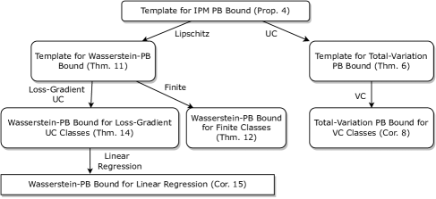
Figure 1: Claims tree diagram. $A\to B$ means that claim $B$ is a special case of claim $A$, under additional assumptions on the learning problem. For full description of the assumptions, see the corresponding claims.

2 Preliminaries

2.1 The Learning Problem

We begin with a short description a standard supervised learning task. Consider a domain $\mathcal{Z}$, a distribution $\mathcal{D}$ over $\mathcal{Z}$, a hypothesis set $\mathcal{H}$, and finally, a loss function $\ell:\mathcal{H}\times\mathcal{Z}\rightarrow[0,1]$. The tuple $(\mathcal{D},\mathcal{H},\ell)$ defines a learning problem: The learning algorithm receives as input a training set $S=\left\{z_{i}\right\}_{i=1}^{m}\in\mathcal{Z}^{m}$ sampled i.i.d from $\mathcal{D}$ and selects an hypothesis $h\in\mathcal{H}$. The performance of $h$ is measured by the expected risk, $L_{\mathcal{D}}(h)\stackrel{{\scriptstyle\text{def}}}{{=}}\mathbb{E}_{z\sim\mathcal{D}}\ell\left(h,z\right)$. While the expected risk is unavailable to algorithm, the empirical risk, $\hat{L}_{S}(h)\stackrel{{\scriptstyle\text{def}}}{{=}}{\displaystyle}\frac{1}{m}\sum_{i=1}^{m}\ell\left(h,z_{i}\right)$, can be evaluated using the training data. The generalization gap is defined by $\Delta_{S}(h)\stackrel{{\scriptstyle\text{def}}}{{=}}L_{\mathcal{D}}(h)-\hat{L}_{S}(h)$.

Several of our results will assume that the learning problem $(\mathcal{D},\mathcal{H},\ell)$ satisfies the uniform convergence property; i.e. the existence of a uniform upper bound on the generalization gap which applies simultaneously to all hypotheses in $\mathcal{H}$.

Definition 1 (Uniform convergence, (Vapnik & Chervonenkis, 2015)).

The learning problem $(\mathcal{D},\mathcal{H},\ell)$ satisfies the uniform convergence property, if there exists a bound function $u(m,\delta^{\prime})>0$ s.t. for any $m\in\mathbb{N}^{+}$, $\delta\in(0,1)$ we have

$$\mathbb{P}\left\{\lvert\Delta_{S}(h)\rvert\leq u(m,\delta),\forall h\in\mathcal{H}\right\}\geq 1-\delta\quad\text{ and }\quad u(m,\delta)\underset{m\to\infty}{\to}0.$$ (1)

UC type bounds are a major part of the foundations of theoretical machine learning. Unfortunately, they suffers from a few drawbacks. First, currently known bounds tend to be extremely loose in many cases, most notably for deep networks. Second, the setup does not provide a natural way to encode prior knowledge into the bounds, particularly when dealing with deep networks - the hypothesis set is usually rich enough to express all relevant functions, and the training algorithms that might utilize some prior knowledge are not themselves a part of UC based bounds. Finally, UC bounds are usually not data-dependent, a property which is critical to explain the generalization of DNNs on real-world data (C. Zhang et al., 2017; Nagarajan & Kolter, 2019b).

2.2 PAC-Bayes Bounds

Let $\mathcal{M}(\mathcal{H})$ denote the set of all probability measures over $\mathcal{H}$. For any probability measure $Q\in\mathcal{M}(\mathcal{H})$, we define the expected loss, empirical loss and generalization gap by

$$L_{\mathcal{D}}(Q) \stackrel{{\scriptstyle\text{def}}}{{=}}\underset{h\sim Q\,\,}{\mathbb{E}}L_{\mathcal{D}}(h)\quad;\quad\hat{L}_{S}(Q)\stackrel{{\scriptstyle\text{def}}}{{=}}\underset{h\sim Q\,\,}{\mathbb{E}}\hat{L}_{S}(h)\quad;\quad\Delta_{S}(Q)\stackrel{{\scriptstyle\text{def}}}{{=}}L_{\mathcal{D}}(Q)-\hat{L}_{S}(Q).$$ (2)

PAC-Bayes theory bounds the expected loss, simultaneously for all “posterior" (sample-dependent) probability measures $Q\in\mathcal{M}(\mathcal{H})$, with high probability over the samples $S\sim\mathcal{D}^{m}$, given any “prior" (sample-independent) probability measure $P\in\mathcal{M}(\mathcal{H})$. A key feature of most PAC-Bayes bounds is their dependence on the KL divergence between the two distributions $P,Q$, $\mathtt{KL}(Q\;\|\;P)\stackrel{{\scriptstyle\text{def}}}{{=}}\int_{\mathcal{H}}\ln(\frac{\mathrm{d}Q}{\mathrm{d}P})\mathrm{d}Q$, where $\frac{\mathrm{d}Q}{\mathrm{d}P}$ is the Radon–Nikodym derivative of $Q$ w.r.t. $P$. While KL is a natural measure of divergence between probability distributions, it restricts the applicability of the resulting bounds to cases where the support of $Q$ is contained in the support of $P$. The following bound was introduced by McAllester (1998).

Proposition 2 (Classical KL-PB Bound).

For any prior $P\in\mathcal{M}(\mathcal{H})$ and $\delta\in(0,1)$, with probability at least $1-\delta$ over the samples $S\sim\mathcal{D}^{m}$, for all $Q\in\mathcal{M}(\mathcal{H})$, we have

$$\Delta_{S}(Q)\leq\sqrt{\frac{\mathtt{KL}(Q\;\|\;P)+\ln(\nicefrac{{m}}{{\delta}})}{2(m-1)}}.$$ (3)

3 A Template for IPM PAC-Bayes Bounds

3.1 General IPM-PB Bound

Definition 3 (Integral Probability Metric).

(Müller, 1997; Sriperumbudur et al., 2009, 2012) The Integral Probability Metric (IPM) between two probability measures $P$ and $Q$ over $\mathcal{H}$ is defined as

$$\gamma_{\mathcal{F}}(Q,P)\stackrel{{\scriptstyle\text{def}}}{{=}}\sup_{f\in\mathcal{F}}\left\lvert\int_{\mathcal{H}}f\mathrm{d}P-\int_{\mathcal{H}}f\mathrm{d}Q\right\rvert=\sup_{f\in\mathcal{F}}\left\lvert\underset{h\sim P\,\,}{\mathbb{E}}\left[f(h)\right]-\underset{h\sim Q\,\,}{\mathbb{E}}\left[f(h)\right]\right\rvert,$$ (4)

where $\mathcal{F}$ is a set of real-valued bounded functions $\mathcal{H}\to\mathbb{R}$.

By definition, IPM distance measures are symmetric and non-negative. Note that the KL-divergence is not a special case of IPM, rather it belongs to the family of $f$-divergences, that intersect with IPM only at the Total-Variation (Sriperumbudur et al., 2009, 2012).

The following proposition assumes that for any fixed sample $S^{\prime}\in\mathcal{Z}^{m}$, the function $f_{S^{\prime}}(h)\stackrel{{\scriptstyle\text{def}}}{{=}}2(m-1)\Delta_{S^{\prime}}^{2}(h)$ is a member of a family of functions that depend on the sample, denoted $\mathcal{F}_{S^{\prime}}$. Thus, the IPM-PB bound allows us to ‘convert’ some knowledge we have about the properties of the generalization gap function $\Delta_{S}(h)$ to a generalization bound.

Since we do not specify yet the collection of function families $\left\{\mathcal{F}_{S}\right\}_{S\in\mathcal{Z}^{m}}$, the bound does not convey an explicit rate, and it should rather be seen as a template. In the next sections, we will derive explicit bounds with specific IPMs divergences. Namely, we will derive a total-variation distance based bound by selecting a collection of bounded function sets, and a Wasserstein distance based bound, by selecting a collection of Lipschitz function sets.

Proposition 4 (Template for IPM PB Bound).

For any fixed dataset $S^{\prime}\in\mathcal{Z}^{m},m\in\mathbb{N}^{+}$, let $\mathcal{F}_{S^{\prime}}$ be a family of bounded and measurable functions $\mathcal{H}\to\mathbb{R}$. Assume that for any number of samples, $m$, and sample $S^{\prime}\in\mathcal{Z}^{m}$, the function $2(m-1)\Delta_{S^{\prime}}^{2}(\cdot)$ is in $\mathcal{F}_{S^{\prime}}$. Then for any prior $P\in\mathcal{M}(\mathcal{H})$ and $\delta\in(0,1)$, with probability at least $1-\delta$ over the samples $S\sim\mathcal{D}^{m}$, for all $Q\in\mathcal{M}(\mathcal{H})$, we have

$$\Delta_{S}(Q)\leq \sqrt{\frac{\gamma_{\mathcal{F}_{S}}(Q,P)+\ln(\nicefrac{{m}}{{\delta}})}{2(m-1)}}.$$ (5)

The proof is in Appendix A.1. The main idea is to use the IPM definition and the assumption as a change-of-measure inequality, instead of the variational formula by Donsker & Varadhan (1975), which is used in the classical KL-PB bound proof. The rest of the proof is similar to the classical derivation (McAllester, 2003; Shalev-Shwartz & Ben-David, 2014).

Note that, similarly to the classical KL-PB bound, Proposition 4 does not require the UC property to hold. However, in the next sections we will see that assuming an existence of a UC bound $u(m,\delta)$, and selecting a particular collection of function families $\left\{\mathcal{F}_{S}\right\}_{S\in\mathcal{Z}^{m}}$, will result in explicit bounds that can improve upon the worst-case nature of the original $u(m,\delta)$ bound.

3.2 Template for Seeger Type IPM PAC-Bayes Bound

The work of Seeger (2002) and Maurer (2004) presented a different form of the PAC-Bayes theorem with fast $O(\nicefrac{{1}}{{m}})$ rate as the dominant term, if the empirical risk is low.

We denote by $\mathtt{kl}(p\;\|\;q)$ the KL divergence between two Bernoulli distributions $\mathcal{B}(p)$ and $\mathcal{B}(q)$, $p,q\in[0,1]$, that is,

$$\mathtt{kl}(p\;\|\;q)\stackrel{{\scriptstyle\text{def}}}{{=}}\begin{cases}p\ln\left(\frac{p}{q}\right)+(1-p)\ln\left(\frac{1-p}{1-q}\right),&\text{if $q\notin\{0,1\}$}\\ 0,&\text{else if $p=q$}\\ \text{undefined},&\text{else.}\end{cases}$$ (6)

For any $h\in\mathcal{H}$, define the relative entropy of the empirical risk with respect to the expected one as $\Delta^{\mathtt{kl}}_{S}(h)\stackrel{{\scriptstyle\text{def}}}{{=}}\mathtt{kl}(\hat{L}_{S}(h)\;\|\;L_{D}(h))$. Similarly, and overloading notations, we define for any distribution $Q\in\mathcal{M}(\mathcal{H})$, $\Delta^{\mathtt{kl}}_{S}(Q)\stackrel{{\scriptstyle\text{def}}}{{=}}\mathtt{kl}(\hat{L}_{S}(Q)\;\|\;L_{D}(Q)).$

By replacing the KL-based change-of-measure inequality step in the proof of (Maurer, 2004, Thm. 5) with the IPM property (Def. 3) we get a similar bound for IPM measures (see a detailed proof in Appendix A.2).

Proposition 5 (Template for Seeger Type IPM PAC-Bayes Bound).

Assume $f_{S}(h)\stackrel{{\scriptstyle\text{def}}}{{=}}m\cdot\Delta^{\mathtt{kl}}_{S}(h)\in\mathcal{F}_{S}$. Then for any prior $P\in\mathcal{M}(\mathcal{H})$ and $\delta\in(0,1)$, with probability at least $1-\delta$ over the samples $S\sim\mathcal{D}^{m}$, for all $Q\in\mathcal{M}(\mathcal{H})$, we have

$$\Delta^{\mathtt{kl}}_{S}(Q) \leq\frac{\gamma_{\mathcal{F}_{S}}(Q,P)+\ln(\nicefrac{{{2\sqrt{m}}}}{{\delta}})}{m}.$$ (7)

By applying the Refined Pinsker’s relaxation (McAllester (2003), Eq. 6) we can immediately derive the following, looser, but easier to interpret bound

$$\Delta_{S}(Q) \leq\sqrt{2\hat{L}_{S}(Q)\frac{\gamma_{\mathcal{F}_{S}}(Q,P)+\ln(\nicefrac{{{2\sqrt{m}}}}{{\delta}})}{m}}+2\frac{\gamma_{\mathcal{F}_{S}}(Q,P)+\ln(\nicefrac{{{2\sqrt{m}}}}{{\delta}})}{m}.$$ (8)

When $\hat{L}_{S}(Q)$ is small (as is typical with modern deep networks), the final term determines the convergence rate. We defer the investigation of PB bounds derived from Prop. 5 to Appendix B. In the following sections we focus on investigating the implication of the Template IPM PB Bound of Prop. 4.

4 Total-Variation PAC-Bayes Bounds

In this section, we investigate a PB bound with the total-variation (TV) distance, $D_{\mathrm{TV}}(Q,P)\stackrel{{\scriptstyle\text{def}}}{{=}}\sup_{A\in\Sigma_{\mathcal{H}}}\left\lvert P(A)-Q(A)\right\rvert$, where $\Sigma_{\mathcal{H}}$ is the standard Borel sigma-algebra associated with $\mathcal{H}$. The TV distance can be described as an IPM with the family of functions

$$\mathcal{F}^{\infty}_{M}\stackrel{{\scriptstyle\text{def}}}{{=}}\left\{f:\mathcal{H}\to[0,\infty),\left\|f\right\|_{\infty}\leq M\right\},$$ (9)

for any $M\geq 0$. To see this, note that

$$\gamma_{\mathcal{F}^{\infty}_{M}}(Q,P)=\sup_{f\in\mathcal{F}^{\infty}_{M}}\left\lvert\int_{\mathcal{H}}f\mathrm{d}P-\int_{\mathcal{H}}f\mathrm{d}Q\right\rvert\stackrel{{\scriptstyle\textit{\text{(i)}}}}{{=}}M\cdot\sup_{A\in\Sigma_{\mathcal{H}}}\left\lvert P(A)-Q(A)\right\rvert=MD_{\mathrm{TV}}(Q,P),$$ (10)

where equality (i) holds since in the supremum it suffices to take the class of indicator functions $\left\{M\cdot\mathbb{1}_{A}(h),A\in\Sigma_{\mathcal{H}}\right\}$, since the functions in $\mathcal{F}^{\infty}_{M}$ are bounded in $[0,M]$.

Theorem 6 (Template for Total-Variation PB Bound).

Assume that there exists some uniform convergence bound $u(m,\delta^{\prime})$ (Definition 1), then, for any prior $P\in\mathcal{M}(\mathcal{H})$ and $\delta\in\left(0,1\right)$, with probability of at least $1-\delta$ over samples $S\sim\mathcal{D}^{m}$, for all $Q\in\mathcal{M}(\mathcal{H})$, we have

$$\Delta_{S}(Q)\leq\sqrt{u^{2}(m,\nicefrac{{\delta}}{{2}})D_{\mathrm{TV}}(Q,P)+\frac{\ln(\nicefrac{{2m}}{{\delta}})}{2(m-1)}}.$$ (11)

The proof (Appendix A.3) follows directly from the general IPM PB bound (Prop. 4) and the uniform convergence assumption, using a union bound argument. This bound can be seen as a template to be used to derive explicit PB bounds, by plugging in existing UC bounds. Note that while we require the existence of UC bound, the resulting bound is nonuniform (since it depends on the data-dependent posterior).

Compared to the original UC bound, $u(m,\delta)$, the bound in (11) is roughly multiplied by a factor of $\sqrt{D_{\mathrm{TV}}(Q,P)}\in[0,1]$, ensuring tighter guarantees, especially if the posterior is close to the prior.

For example, consider a binary classification case, with the zero-one loss function and $\mathtt{VC}(\mathcal{H})$ class ${\cal H}$. The well-known UC theorem states that the generalization gap converges uniformly at a rate $O\left(\sqrt{\nicefrac{{\mathtt{VC}(\mathcal{H})}}{{m}}}\right)$.

Proposition 7 (VC Bound, Boucheron et al. (2005)).

There exists some universal constant $c>0$ s.t. for any $\delta\in(0,1)$ we have

$$\mathbb{P}\left\{\Delta_{S}(h)\leq c\sqrt{\frac{\mathtt{VC}(\mathcal{H})+\ln(\nicefrac{{1}}{{\delta}})}{m}},\forall h\in\mathcal{H}\right\}\geq 1-\delta.$$ (12)

Using Thm. 6, we derive the following algorithm and data-dependent bound.

Corollary 8 (Total-Variation PB Bound for VC Classes).

Consider a binary classification problem, with the zero-one loss, and hypothesis class $\mathcal{H}$, with finite VC dimension, $\mathtt{VC}(\mathcal{H})$. There exists some universal constant $c>0$ s.t. for any prior $P\in\mathcal{M}(\mathcal{H})$ and $\delta\in\left(0,1\right)$, with probability of at least $1-\delta$ over samples $S\sim\mathcal{D}^{m}$, for all $Q\in\mathcal{M}(\mathcal{H})$, we have

$$\Delta_{S}(Q)\leq\sqrt{c\frac{\mathtt{VC}(\mathcal{H})+\ln(\nicefrac{{1}}{{\delta}})}{m}D_{\mathrm{TV}}(Q,P)+\frac{\ln(\nicefrac{{m}}{{\delta}})}{2(m-1)}}.$$ (13)

Compared to the UC bound of Prop. 7, Cor. 8 multiplies the dominant term of the bound by a nonuniform (data and algorithm-dependent) factor of $\sqrt{D_{\mathrm{TV}}(Q,P)}$, which is guaranteed to tighten the bound.

Note that the total-variation based bound of Aminian et al. (2022) and Rodríguez Gálvez et al. (2021) assume Lipschitz loss function, while our TV bound allows non continuous loss functions such as the zero-one loss. The TV based bound of Wang et al. (2019) (Thm. 1) is not directly comparable, since the empirical risk term is multiplied by a factor that goes to infinity for TV distance that goes to 1.

5 Wasserstein PAC-Bayes Bounds

5.1 Template for Wasserstein-PB Bound

In this section, we provide a PAC-Bayes generalization bound with the Wasserstein metric between posterior and prior and a certain smoothness parameter of the generalization gap function. We explore learning settings for which $\mathcal{H}$ can be paired with a distance metric $\rho:\mathcal{H}\times\mathcal{H}\to\mathbb{R}_{\geq 0}$ s.t. $\left(\mathcal{H},\rho\right)$ is a Polish metric space (complete, separable metric space). Given the distance metric $\rho$, we can define the Wasserstein distance between any two probability measures on $\mathcal{H}$.

Definition 9 (Wasserstein Distance).

For any two probability measures $P,Q$ on $\mathcal{H}$ with finite first moment, the $1^{\mbox{st}}$ order Wasserstein distance is

$$W_{1}(Q,P) \stackrel{{\scriptstyle\text{def}}}{{=}}\inf_{\gamma\in\Gamma(Q,P)}\int_{\mathcal{H}\times\mathcal{H}}\rho(h,h^{\prime})\mathrm{d}\gamma(h,h^{\prime}),$$ (14)

where $\Gamma(Q,P)$ denotes the set of all couplings of $Q$ and $P$, that is, the set of all joint measure on $\mathcal{H}\times\mathcal{H}$ whose marginals are $Q$ and $P$.

The following proposition gives a dual representation for the first-order Wasserstein distance.

Proposition 10 (Kantorovich-Rubinstein Duality (Villani, 2006)).

For any $0\leq K$, and any two probability measures $P,Q\in\mathcal{M}(\mathcal{H})$,

$$K\cdot W_{1}(Q,P)=\sup_{f\in\mathcal{F}^{\text{Lip}}_{K}}\left\lvert\underset{h\sim P\,\,}{\mathbb{E}}\left[f(h)\right]-\underset{h\sim Q\,\,}{\mathbb{E}}\left[f(h)\right]\right\rvert,$$ (15)

where $\mathcal{F}^{\text{Lip}}_{K}$ is the set of $K$-Lipschitz functions w.r.t. $\rho(h,h^{\prime})$, i.e. functions that satisfy

$$\sup_{(h,h^{\prime})\in\mathcal{H}^{2}}\frac{\left\lvert f(h)-f(h^{\prime})\right\rvert}{\rho(h,h^{\prime})}\leq K.$$ (16)

We can write the Kantorovich-Rubinstein duality (15) using IPM formulation (Def. 3),

$$K\cdot W_{1}(Q,P)=\gamma_{\mathcal{F}^{\text{Lip}}_{K}}(P,Q).$$ (17)

Using this duality we will prove the following bound.

Theorem 11 (Template for Wasserstein-PB Bound).

Assume that for any $\delta^{\prime}\in(0,1]$, w.p. at least $1-\delta^{\prime}$ over the sampling $S\sim\mathcal{D}^{m}$, the squared generalization gap function, $\Delta_{S}^{2}(\cdot)$, is $K$-Lipschitz w.r.t. the metric $\rho$ with some $K=K(m,\delta^{\prime})$. Then, for any prior $P\in\mathcal{M}(\mathcal{H})$ and $\delta\in\left(0,1\right)$, with probability of at least $1-\delta$ over samples $S\sim\mathcal{D}^{m}$, for all $Q\in\mathcal{M}(\mathcal{H})$, we have

$$\Delta_{S}(Q)\leq\sqrt{K(m,\nicefrac{{\delta}}{{2}})W_{1}(Q,P)+\frac{\ln(\nicefrac{{2m}}{{\delta}})}{2(m-1)}}.$$ (18)

The proof (Appendix A.4) follows directly from Proposition 4 and the assumption, via the union bound. Theorem 11 can be seen as a template to be used for deriving Wasserstein-PB bounds in various learning settings where the $\Delta_{S}^{2}(\cdot)$ is $K$-Lipschitz with high probability (over samples), where the rate of $K=K(m,\nicefrac{{\delta}}{{2}})$ should be $O(\nicefrac{{1}}{{m}})$ to ensure a factor $O(\nicefrac{{1}}{{\sqrt{m}}})$ multiplying the divergence between posterior and prior, as in the KL-PB bound.

Such a result can be challenging to prove since it requires uniform convergence of the slope between any two hypotheses in $\mathcal{H}$. Next, we will show specific learning settings where this property holds and the resulting generalization bounds.

We note that recent work Neu & Lugosi (2022) also establishes a Wasserstein-based information-theoretic generalization bound. This work assumed infinitely smooth loss functions and established bounds on the expected generalization gap, rather than high-probability bounds. In fact, Neu & Lugosi (2022) noted that obtaining such bounds is an open problem. Observe, though, that our bound depends on the Lipschitz constant $K=K(m,\delta)$ which needs to assessed; see sections 5.2 and 5.3 for specific examples. The general problem remains open.

At a more pragmatic level, we note that learning algorithms derived from minimizing Wasserstein based PB bounds have an added benefit of more stable optimization compared to KL based approaches, due to lower gradient variance, as noted in Arjovsky et al. (2017), and this distance measure can be approximated efficiently from finite samples (Weed & Bach, 2017; Cuturi, 2013)

5.2 Wasserstein-PB Bound for Finite Classes

We first investigate the simple case of a finite hypothesis class with a loss function $\ell$ which is $G$-Lipschitz w.r.t. the metric $\rho$. Note that for finite classes, UC always holds. We derive the following bound from Thm. 11.

Theorem 12 (Wasserstein-PB Bound for Finite Classes).

Let $\mathcal{H}$ be a finite hypothesis class. Assume that for any fixed $z\in\mathcal{Z}$, $\ell(h,z)$ is a $G$-Lipschitz function in $h$ w.r.t the metric $\rho$. Then for any prior $P\in\mathcal{M}(\mathcal{H})$ and $\delta\in\left(0,1\right)$, with probability of at least $1-\delta$ over samples $S\sim\mathcal{D}^{m}$, for all $Q\in\mathcal{M}(\mathcal{H})$, we have

$$\Delta_{S}(Q)\leq\sqrt{\frac{8G\log(\nicefrac{{4\lvert\mathcal{H}\rvert}}{{\delta}})}{m}W_{1}(Q,P)+\frac{\ln(\nicefrac{{2m}}{{\delta}})}{2(m-1)}}.$$ (19)

The proof (Appendix A.5) makes use of standard union bound arguments, Hoeffding’s concentration inequality and the template Wasserstein-PB bound (Thm. 11). Notice that compared to the standard UC bound for finite classes, Thm. 12 multiplies the bound by a nonuniform factor of $\sqrt{GW_{1}(Q,P)}$.

5.3 Wasserstein-PB Bound for Loss-Gradient UC Classes

In this section we show a Wasserstein-PB bound for learning problems $(\mathcal{D},\mathcal{H},\ell)$, with $\mathcal{H}\subset\mathbb{R}^{d}$, for some dimension $d\in\mathbb{N}^{+}$, that satisfy the standard UC property, and, additionally, satisfy UC property for the loss gradient, as defined below.

Definition 13 (Loss-Gradient UC Property).

A learning problem $(\mathcal{D},\mathcal{H},\ell)$, with $\mathcal{H}\subset\mathbb{R}^{d}$, is said to satisfy the loss-gradient UC property, if: (i) the loss function $\ell(h,z)$ is differentiable w.r.t. h on $\text{Int}(\mathcal{H})\times\mathcal{Z}$ and continuous w.r.t. $h$ on $\mathcal{H}\times\mathcal{Z}$. (ii) The problem satisfies the uniform convergence property (Def. 1). (iii) The empirical average of the loss gradient converges uniformly in $L_{2}$ norm sense to its mean. I.e., there exists a bound function $u^{\text{grad}}(m,\delta)>0$, s.t. for any $\delta\in(0,1)$ we have $u^{\text{grad}}(m,\delta)\underset{m\to\infty}{\to}0$ and for any $m\in\mathbb{N}^{+}$,

$$\mathbb{P}\left(\left\|\mathbb{E}_{z\sim\mathcal{D}}\nabla_{h}\ell(h,z)-\frac{1}{m}\sum_{i=1}^{m}\nabla_{h}\ell(h,z_{i})\right\|_{2}\leq u^{\text{grad}}(m,\delta),\forall h\in\text{Int}(\mathcal{H})\right)\geq 1-\delta,$$ (20)

where $\nabla_{h}\ell(h,z)$ denotes the gradient of $\nabla_{h}\ell(h,z)$ w.r.t. $h$, for a fixed $z\in\mathcal{Z}$, and $\text{Int}(\mathcal{H})$ is the interior of $\mathcal{H}$. We call $u^{\text{grad}}$, the UC bound of the loss gradient.

Theorem 14 (Wasserstein-PB Bound for Loss-Gradient UC Classes).

Let $(\mathcal{H},\rho)$ be a metric space such that $\mathcal{H}\subset\mathbb{R}^{d}$ is a closed and convex set, and $\rho$ is the $L_{2}$ distance. Assume the learning problem satisfies the loss-gradient UC property (Def. 13), with UC bound $u$, and a UC bound of the loss gradient, $u^{\text{grad}}$. Then for any prior $P\in\mathcal{M}(\mathcal{H})$ and $\delta\in\left(0,1\right)$, with probability of at least $1-\delta$ over samples $S\sim\mathcal{D}^{m}$, for all $Q\in\mathcal{M}(\mathcal{H})$, we have

$$\Delta_{S}(Q)\leq\sqrt{2\cdot u(m,\nicefrac{{\delta}}{{4}})\cdot u^{\text{grad}}(m,\nicefrac{{\delta}}{{4}})\cdot W_{1}(Q,P)+\frac{\ln(\nicefrac{{2m}}{{\delta}})}{2(m-1)}}.$$ (21)

The proof (Appendix A.6) is derived from the assumptions and the template Wasserstein-PB bound (Thm. 11). In learning problems that satisfy the loss-gradient UC property, we often have $u(m,\nicefrac{{\delta}}{{4}}),u^{\text{grad}}(m,\nicefrac{{\delta}}{{4}})\in O(\nicefrac{{1}}{{\sqrt{m}}})$, and then the resulting bound is $O(\nicefrac{{1}}{{\sqrt{m}}})$. We provide full analysis that shows such a rate for the following linear regression example.

5.4 Linear Regression Example

Based on the Wasserstein-PB Bound for Loss-Gradient UC Classes (Thm. 14), we derive the following corollary.

Corollary 15 (Wasserstein-PB Bound for Linear Regression).

Consider a data distribution of pairs $z=(x,y)$, where $x$ is sampled from an unknown distribution supported on a $d$-dimensional ball of radius $r>0$, $\mymathbb{B}^{d}_{r}\stackrel{{\scriptstyle\text{def}}}{{=}}\{x\in\mathbb{R}^{d}:\left\|x\right\|_{2}\leq r\}$, and the target, $y=f(x)$, is set by an unknown, possibly random, target function $f:\mymathbb{B}^{d}_{r}\to[-1,1]$. The hypothesis space $\mathcal{H}$ is $\mymathbb{B}^{d}_{\nicefrac{{1}}{{r}}}$ , and the loss function is $\ell(x,y,h)=\frac{1}{4}(h^{\top}x-y)^{2}$. Then, for any prior $P\in\mathcal{M}(\mathcal{H})$ and $\delta\in\left(0,1\right)$, with probability at least $1-\delta$ over samples $S\sim\mathcal{D}^{m}$, for all $Q\in\mathcal{M}(\mathcal{H})$,

$$\Delta_{S}(Q)\leq\sqrt{2u(m,\nicefrac{{\delta}}{{4}})\cdot u^{\text{grad}}(m,\nicefrac{{\delta}}{{4}})\cdot W_{1}(Q,P)+\frac{\ln(\nicefrac{{2m}}{{\delta}})}{2(m-1)}},$$ (22)

where $W_{1}(Q,P)$ denotes the $1^{\mbox{st}}$ order Wasserstein distance with the $L_{2}$ metric,

$$u(m,\delta)\in O\left(\sqrt{\frac{d\left(1+\ln(\nicefrac{{1}}{{\delta}}\right))}{m}}\right)\text{, and }u^{\text{grad}}(m,\delta)\in O\left(r\sqrt{\frac{d\left(1+\ln(\nicefrac{{1}}{{\delta}}\right))}{m}}\right).$$ (23)

The full expression of the bound appears in the theorem’s proof (Appendix A.7). Ignoring logarithmic factors we obtained a UC bound of $\tilde{O}\left(\sqrt{\frac{d}{m}}\right)$, and a Wasserstein-PB bound of $\tilde{O}\left(\sqrt{rW_{1}(Q,P)\frac{d}{m}}\right)$. Note that from Thm. 6 we can also deduce a TV-PB bound of order $\tilde{O}\left(\sqrt{D_{\mathrm{TV}}(Q,P)\frac{d}{m}}\right)$. In comparison, the standard KL-PB bound is of order $\tilde{O}\left(\sqrt{\frac{\mathtt{KL}(Q\;\|\;P)}{m}}\right)$. The TV-PB bound is, at worst, roughly the same as the UC bound, since $D_{\mathrm{TV}}(Q,P)\leq 1$. Note that since $Q$ and $P$ are distributions over a sphere of radius $\nicefrac{{1}}{{r}}$, then $rW_{1}(Q,P)\leq 2$. Hence, the Wasserstein-PB is also, at worst, roughly the same as the UC bound. However, the KL-PB bound can be either tighter or looser, depending on $P$ and $Q$. In cases where the mass of the posterior $Q$ is concentrated in a region of the hypothesis set where the prior $P$ is arbitrarily small, then the KL divergence can be arbitrarily large, making the KL-PB bound extremely loose compared to the UC, TV-PB, and Wasserstein-PB bounds. The numerical experiment described in Appendix C demonstrates this by investigating different prior distributions with different widths. In particular, for posteriors and priors that are Dirac delta distributions (i.e., deterministic predictors), we show that the Wasserstein-PB considerably improves over the UC bound, while the KL-PB bound is undefined. We therefore demonstrated non-vacuous guarantees for deterministic models within the PB framework without requiring additional derandomization steps.

We can compare the bound of Thm. 14 to the bound of Corollary 8, in Neu & Lugosi (2022), which is also dependent on the Wasserstein distance between a data-dependent output (posterior) and a base measure (prior). The bound of Thm. 14 is different in the sense that (i) It holds with high probability instead of in expectation. (ii) Instead of assuming infinitely-smooth loss function with $\beta$-bounded directional derivatives, Thm. 14 assumes a loss-gradient UC class. (iii) The bound scales as $\tilde{O}\left(\sqrt{W_{1}\cdot u\cdot u^{\text{grad}}}\right)$ instead of $\tilde{O}\left(\sqrt{W_{2}\cdot\frac{d\beta}{m}}\right)$.

In our linear regression example, Cor. 15 scales as $\tilde{O}\left(\sqrt{W_{1}\cdot u\cdot u^{\text{grad}}}\right)=\tilde{O}\left(\sqrt{r\sqrt{\frac{d}{m}}r\sqrt{\frac{d}{m}}}\right)=\tilde{O}\left(r\sqrt{\frac{d}{m}}\right)$. The loss is infinitely-smooth with $\beta\in O(1+r+r^{2})$, and therefore Cor. 8 of Neu & Lugosi (2022) scales as $\tilde{O}\left(\sqrt{W_{2}\cdot\frac{d\beta}{m}}\right)=\tilde{O}\left(r\sqrt{\frac{d}{m}(1+r+r^{2})}\right)$, i.e., looser by a factor of $\tilde{O}\left(\sqrt{1+r+r^{2}}\right)$ compared to Cor. 15.

6 Discussion

We have presented high-probability PB bounds based on integral probability metrics, that extend standard PB bounds based on KL divergence and more recent $f$-divergence and $\alpha$-divergence based bounds, to a new class of distances. Our bounds interpolate between classic UC bounds and PB bounds, by allowing data- and algorithm-dependent complexity terms. As in all PB results, our bounds suggest improved rates when the PB posterior is close to the prior. While we have extended high-probability PB bounds for IPMs to novel distance measures, it is still an open question to do so without the UC assumption.

Possible directions for future research include: (i) Deriving high probability IPM-PB bounds (e.g. Wasserstein or TV based), without global UC assumptions (possibly using localization based approaches, e.g. , Local Rademacher complexities (Koltchinskii & Panchenko, 2004; Bartlett et al., 2005) are computed only on a subset of hypotheses with small empirical risk). This may allow non-vacuous bounds for large-scale models where global UC-based bounds are extremely vacuous. (ii) Derivation of algorithms that utilize the bounds as minimization objectives. Based on the optimization advantages of Wasserstein based costs mentioned in Sec. 5.1, these could lead to enhanced practical utility. Such an advantage could play an important role in meta-learning schemes where PB methods have been widely used in recent years (Amit and Meir, 2018).

Acknowledgments

We thank Nadav Merlis and Daniel Soudry for helpful discussions of this work, and the anonymous reviewers for their helpful comments. Shay Moran is a Robert J. Shillman Fellow; he acknowledges support by ISF grant 1225/20, by BSF grant 2018385, by an Azrieli Faculty Fellowship, by Israel PBC-VATAT, by the Technion Center for Machine Learning and Intelligent Systems (MLIS), and by the the European Union (ERC, GENERALIZATION, 101039692). Views and opinions expressed are however those of the author(s) only and do not necessarily reflect those of the European Union or the European Research Council Executive Agency. Neither the European Union nor the granting authority can be held responsible for them. The work of Ron Meir is partially supported by ISF grant 1693/22, by the Ollendorff Center of the Viterbi ECE Faculty at the Technion, and by the Skillman chair in biomedical sciences.

Checklist

1. For all authors…

   1. Do the main claims made in the abstract and introduction accurately reflect the paper’s contributions and scope? [Yes]

   2. Did you describe the limitations of your work? [Yes]

   3. Did you discuss any potential negative societal impacts of your work? [N/A]

   4. Have you read the ethics review guidelines and ensured that your paper conforms to them? [Yes]

2. If you are including theoretical results…

   1. Did you state the full set of assumptions of all theoretical results? [Yes]

   2. Did you include complete proofs of all theoretical results? [Yes]

3. If you ran experiments…

   1. Did you include the code, data, and instructions needed to reproduce the main experimental results (either in the supplemental material or as a URL)? [Yes]

   2. Did you specify all the training details (e.g., data splits, hyperparameters, how they were chosen)? [Yes]

   3. Did you report error bars (e.g., with respect to the random seed after running experiments multiple times)? [Yes]

   4. Did you include the total amount of compute and the type of resources used (e.g., type of GPUs, internal cluster, or cloud provider)? [N/A]

4. If you are using existing assets (e.g., code, data, models) or curating/releasing new assets…

   1. If your work uses existing assets, did you cite the creators? [N/A]

   2. Did you mention the license of the assets? [N/A]

   3. Did you include any new assets either in the supplemental material or as a URL? [N/A]

   4. Did you discuss whether and how consent was obtained from people whose data you’re using/curating? [N/A]

   5. Did you discuss whether the data you are using/curating contains personally identifiable information or offensive content? [N/A]

5. If you used crowdsourcing or conducted research with human subjects…

   1. Did you include the full text of instructions given to participants and screenshots, if applicable? [N/A]

   2. Did you describe any potential participant risks, with links to Institutional Review Board (IRB) approvals, if applicable? [N/A]

   3. Did you include the estimated hourly wage paid to participants and the total amount spent on participant compensation? [N/A]

Appendix A Appendix: Proofs

A.1 Proof of the IPM-PB Bound (Prop. 4)

Proof.

The proof follows a similar structure as the classical derivation (McAllester, 2003; Shalev-Shwartz & Ben-David, 2014), except for replacing the change-of-measure inequality.

For any sample $S\in\mathcal{Z}^{m}$, consider the function

$$f_{S}(h)\stackrel{{\scriptstyle\text{def}}}{{=}}2(m-1)\Delta_{S}^{2}(h).$$

Since we assume $f_{S}\in\mathcal{F}_{S}$, Definition 3 implies that for any pair of probability measures $P,Q\in\mathcal{M}(\mathcal{H})$

$$\underset{h\sim Q\,\,}{\mathbb{E}}\left[f_{S}(h)\right]-\underset{h\sim P\,\,}{\mathbb{E}}\left[f_{S}(h)\right] \leq\gamma_{\mathcal{F}_{S}}(Q,P).$$

Therefore, by the monotonicity of $\exp(\cdot)$ we have

$$\exp\left(\underset{h\sim Q\,\,}{\mathbb{E}}\left[f_{S}(h)\right]-\gamma_{\mathcal{F}_{S}}(Q,P)\right) \leq\exp\left(\underset{h\sim P\,\,}{\mathbb{E}}\left[f_{S}(h)\right]\right)$$ (24)

$$\leq\underset{h\sim P\,\,}{\mathbb{E}}\left[\exp\left(f_{S}(h)\right)\right].$$ (25)

where the last inequality is by the convexity of $\exp(\cdot)$, and by Jensen’s inequality.

Taking the supremum over $Q\in\mathcal{M}(\mathcal{H})$, and an expectation over samples $S\sim\mathcal{D}^{m}$ we have that for any $P\in\mathcal{M}(\mathcal{H})$

$$\mathbb{E}_{S\sim\mathcal{D}^{m}}\sup_{Q}\left\{\exp\left(\underset{h\sim Q\,\,}{\mathbb{E}}\left[f_{S}(h)\right]-\gamma_{\mathcal{F}_{S}}(Q,P)\right)\right\} \leq\mathbb{E}_{S\sim\mathcal{D}^{m}}\sup_{Q}\left\{\underset{h\sim P\,\,}{\mathbb{E}}\exp\left(f_{S}(h)\right)\right\}$$ (26)

$$=\mathbb{E}_{S\sim\mathcal{D}^{m}}\underset{h\sim P\,\,}{\mathbb{E}}\exp\left(f_{S}(h)\right)$$

$$=\underset{h\sim P\,\,}{\mathbb{E}}\mathbb{E}_{S\sim\mathcal{D}^{m}}\exp\left(f_{S}(h)\right),$$

where the last equality is obtained by the prior’s independence from the sample, and from Fubini’s theorem. We recall that by Hoeffding’s inequality, for any $h\in\mathcal{H}$,

$$\mathbb{P}_{S\sim\mathcal{D}^{m}}\left(\Delta_{S}(h)>u\right) \leq e^{-2mu^{2}},$$

which, by Lemma 5 of McAllester (2003), this imply.

$$\mathbb{E}_{S\sim\mathcal{D}^{m}}\exp\left(f_{S}(h)\right)=\mathbb{E}_{S\sim\mathcal{D}^{m}}\exp\left(2(m-1)\Delta_{S}^{2}(h)\right)\leq m.$$ (27)

Inequalities (26) and (27) imply

$$\mathbb{E}_{S\sim\mathcal{D}^{m}}\sup_{Q}\left\{\exp\left(\underset{h\sim Q\,\,}{\mathbb{E}}\left[f_{S}(h)\right]-\gamma_{\mathcal{F}_{S}}(Q,P)\right)\right\} \leq m.$$

Therefore, by Markov’s inequality, for any $t>0$ we have

$$\mathbb{P}_{S\sim\mathcal{D}^{m}}\left(\sup_{Q}\left\{\exp\left(\underset{h\sim Q\,\,}{\mathbb{E}}\left[f_{S}(h)\right]-\gamma_{\mathcal{F}_{S}}(Q,P)\right)\right\}\geq t\right) \leq\frac{m}{t}.$$

Or, equivalently,

$$\mathbb{P}_{S\sim\mathcal{D}^{m}}\left(\ln\left(\sup_{Q}\left\{\exp\left(\underset{h\sim Q\,\,}{\mathbb{E}}\left[f_{S}(h)\right]-\gamma_{\mathcal{F}_{S}}(Q,P)\right)\right\}\right)\geq\ln(t)\right) \leq\frac{m}{t}.$$

By Lem. 18, the $\ln(\cdot)$ and $\sup(\cdot)$ operations are interchangeable, and therefore

$$\mathbb{P}_{S\sim\mathcal{D}^{m}}\left(\sup_{Q}\left\{\underset{h\sim Q\,\,}{\mathbb{E}}\left[f_{S}(h)\right]-\gamma_{\mathcal{F}_{S}}(Q,P)\right\}\geq\ln(t)\right) \leq\frac{m}{t}.$$

Let $\delta\in(0,1)$, we set $t=\frac{m}{\delta}$, and plug in $f_{S}(h)\stackrel{{\scriptstyle\text{def}}}{{=}}2(m-1)\Delta_{S}^{2}(h)$ to get

$$\mathbb{P}_{S\sim\mathcal{D}^{m}}\left(\sup_{Q}\left\{\underset{h\sim Q\,\,}{\mathbb{E}}\left(2(m-1)\Delta_{S}^{2}(h)\right)-\gamma_{\mathcal{F}_{S}}(Q,P)\right\}\geq\ln(\nicefrac{{m}}{{\delta}})\right) \leq\delta.$$

Therefore, the complementary event satisfies

$$\mathbb{P}_{S\sim\mathcal{D}^{m}}\left(\sup_{Q}\left\{\underset{h\sim Q\,\,}{\mathbb{E}}\left(2(m-1)\Delta_{S}^{2}(h)\right)-\gamma_{\mathcal{F}_{S}}(Q,P)\right\}<\ln(\nicefrac{{m}}{{\delta}})\right) \geq 1-\delta.$$

I.e., for any $P\in\mathcal{M}(\mathcal{H})$, with a probability of at least $1-\delta$ over the samples $S\sim\mathcal{D}^{m}$, the following inequality holds for all $Q\in\mathcal{M}(\mathcal{H})$

$$\underset{h\sim Q\,\,}{\mathbb{E}}\left(\Delta_{S}^{2}(h)\right) <\frac{\gamma_{\mathcal{F}_{S}}(Q,P)+\ln(\nicefrac{{m}}{{\delta}})}{2(m-1)}.$$

Jensen’s inequality implies that

$$\left(\underset{h\sim Q\,\,}{\mathbb{E}}\Delta_{S}(h)\right)^{2}\leq\underset{h\sim Q\,\,}{\mathbb{E}}\left(\Delta_{S}^{2}(h)\right) \leq\frac{\gamma_{\mathcal{F}}(Q,P)+\ln(\nicefrac{{m}}{{\delta}})}{2(m-1)}.$$

The proof is concluded by taking the square root of both sides. ∎

A.2 Proof of the Seeger’s Type IPM-PB Bound (Prop. 5)

Proof.

As in the proof of Prop. 4, we follow a similar structure as the classical derivation (McAllester, 2003; Maurer, 2004), except replacing the change-of-measure inequality.

For any sample $S\in\mathcal{Z}^{m}$, consider the function on $\mathcal{H}$

$$f_{S}(h)\stackrel{{\scriptstyle\text{def}}}{{=}}m\cdot\mathtt{kl}(\hat{L}_{S}(h)\;\|\;L_{D}(h)).$$

Note that $f_{S}(\cdot)$ is almost surely well-defined, since if $L_{D}(h)=0$, then $\hat{L}(h)\stackrel{{\scriptstyle\textit{\text{a.s.}}}}{{=}}0$.

Since we assume $f_{S}\in\mathcal{F}_{S}$, Definition 3 implies that for any pair of probability measures $P,Q\in\mathcal{M}(\mathcal{H})$

$$\underset{h\sim Q\,\,}{\mathbb{E}}\left[f_{S}(h)\right]-\underset{h\sim P\,\,}{\mathbb{E}}\left[f_{S}(h)\right] \leq\gamma_{\mathcal{F}_{S}}(Q,P).$$

Therefore, by the monotonicity of $\exp(\cdot)$ we have

$$\exp\left(\underset{h\sim Q\,\,}{\mathbb{E}}\left[f_{S}(h)\right]-\gamma_{\mathcal{F}_{S}}(Q,P)\right) \leq\exp\left(\underset{h\sim P\,\,}{\mathbb{E}}\left[f_{S}(h)\right]\right)$$

$$\leq\underset{h\sim P\,\,}{\mathbb{E}}\left[\exp\left(f_{S}(h)\right)\right].$$

where the last inequality is by the convexity of $\exp(\cdot)$ and by Jensen’s inequality.

Taking the supremum over $Q\in\mathcal{M}(\mathcal{H})$, and an expectation over samples $S\sim\mathcal{D}^{m}$ we have for any $P\in\mathcal{M}(\mathcal{H})$

$$\mathbb{E}_{S\sim\mathcal{D}^{m}}\sup_{Q}\left\{\exp\left(\underset{h\sim Q\,\,}{\mathbb{E}}\left[f_{S}(h)\right]-\gamma_{\mathcal{F}_{S}}(Q,P)\right)\right\} \leq\mathbb{E}_{S\sim\mathcal{D}^{m}}\sup_{Q}\left\{\underset{h\sim P\,\,}{\mathbb{E}}\exp\left(f_{S}(h)\right)\right\}$$ (28)

$$=\mathbb{E}_{S\sim\mathcal{D}^{m}}\underset{h\sim P\,\,}{\mathbb{E}}\exp\left(f_{S}(h)\right)$$

$$=\underset{h\sim P\,\,}{\mathbb{E}}\mathbb{E}_{S\sim\mathcal{D}^{m}}\exp\left(f_{S}(h)\right),$$

where the last equality is obtained by the prior’s independence from the sample, and from Fubini’s theorem. Using Maurer (2004), Thm. 1 we have

$$\mathbb{E}_{S\sim\mathcal{D}^{m}}\exp\left(f_{S}(h)\right) =\mathbb{E}_{S\sim\mathcal{D}^{m}}\exp\left(m\cdot\mathtt{kl}(\hat{L}_{S}(h)\;\|\;L_{D}(h))\right)$$ (29)

$$\leq 2\sqrt{m}.$$

Inequalities (28) and (29) imply

$$\mathbb{E}_{S\sim\mathcal{D}^{m}}\sup_{Q}\left\{\exp\left(\underset{h\sim Q\,\,}{\mathbb{E}}\left[f_{S}(h)\right]-\gamma_{\mathcal{F}_{S}}(Q,P)\right)\right\} \leq 2\sqrt{m}.$$

Therefore, by Markov’s inequality, for any $t>0$ we have

$$\mathbb{P}_{S\sim\mathcal{D}^{m}}\left(\sup_{Q}\left\{\exp\left(\underset{h\sim Q\,\,}{\mathbb{E}}\left[f_{S}(h)\right]-\gamma_{\mathcal{F}_{S}}(Q,P)\right)\right\}\geq t\right) \leq\frac{2\sqrt{m}}{t},$$

or, equivalently,

$$\mathbb{P}_{S\sim\mathcal{D}^{m}}\left(\ln\left(\sup_{Q}\left\{\exp\left(\underset{h\sim Q\,\,}{\mathbb{E}}\left[f_{S}(h)\right]-\gamma_{\mathcal{F}_{S}}(Q,P)\right)\right\}\right)\geq\ln(t)\right) \leq\frac{2\sqrt{m}}{t}.$$

By Lem. 18, the $\ln(\cdot)$ and $\sup(\cdot)$ operations are interchangeable, and therefore

Let $\delta\in(0,1)$, we set $t=\frac{2\sqrt{m}}{\delta}$, and plug in $f_{S}(h)\stackrel{{\scriptstyle\text{def}}}{{=}}m\cdot\mathtt{kl}(\hat{L}_{S}(h)\;\|\;L_{D}(h))$ to get

$$\mathbb{P}_{S\sim\mathcal{D}^{m}}\left(\sup_{Q}\left\{m\underset{h\sim Q\,\,}{\mathbb{E}}\mathtt{kl}(\hat{L}_{S}(h)\;\|\;L_{D}(h))-\gamma_{\mathcal{F}_{S}}(Q,P)\right\}\geq\ln(\nicefrac{{2\sqrt{m}}}{{\delta}})\right) \leq\delta.$$

Therefore, the complementary event satisfies

$$\mathbb{P}_{S\sim\mathcal{D}^{m}}\left(\sup_{Q}\left\{m\underset{h\sim Q\,\,}{\mathbb{E}}\mathtt{kl}(\hat{L}_{S}(h)\;\|\;L_{D}(h))-\gamma_{\mathcal{F}_{S}}(Q,P)\right\}<\ln(\nicefrac{{2\sqrt{m}}}{{\delta}})\right) \geq 1-\delta.$$

I.e., for any $P\in\mathcal{M}(\mathcal{H})$, with a probability of at least $1-\delta$ over the samples $S\sim\mathcal{D}^{m}$, the following inequality holds for all $Q\in\mathcal{M}(\mathcal{H})$

$$\underset{h\sim Q\,\,}{\mathbb{E}}\mathtt{kl}(\hat{L}_{S}(h)\;\|\;L_{D}(h)) <\frac{\gamma_{\mathcal{F}_{S}}(Q,P)+\ln(\nicefrac{{{2\sqrt{m}}}}{{\delta}})}{m}.$$

By the convexity of the function $\mathtt{kl}(p\;\|\;q)$ in the pair of parameters $(p,q)$ and by Jensen’s inequality, we have

$$\mathtt{kl}(\underset{h\sim Q\,\,}{\mathbb{E}}\hat{L}_{S}(h)\;\|\;\underset{h\sim Q\,\,}{\mathbb{E}}L_{D}(h))\leq\underset{h\sim Q\,\,}{\mathbb{E}}\mathtt{kl}(\hat{L}_{S}(h)\;\|\;L_{D}(h)).$$

Therefore we finally get that for any $P\in\mathcal{M}(\mathcal{H})$, w.p. of at least $1-\delta$ the following holds for all $Q\in\mathcal{M}(\mathcal{H})$

$$\mathtt{kl}(\hat{L}_{S}(Q)\;\|\;L_{D}(Q)) <\frac{\gamma_{\mathcal{F}_{S}}(Q,P)+\ln(\nicefrac{{{2\sqrt{m}}}}{{\delta}})}{m}.$$

∎

A.3 Proof of the Total-Variation PAC-Bayes Bound (Thm. 6)

Proof.

Let $\delta>0$. For any fixed sample $S\in\mathcal{Z}^{m}$, we define $f_{S}(h)\stackrel{{\scriptstyle\text{def}}}{{=}}2(m-1)\Delta^{2}_{S}(h)$. Define $M_{S}\stackrel{{\scriptstyle\text{def}}}{{=}}\sup_{h\in\mathcal{H}}\Delta^{2}_{S}(h)$. Therefore, $0\leq f_{S}(h)\leq 2(m-1)M_{S}$, i.e., $f_{S}(h)\in\mathcal{F}^{\infty}_{2(m-1)M_{S}}$. This fact, together with the general IPM PB bound (Prop. 4) and Eq. (10) (equivalence of IPM to TV under the family of bounded functions) imply that for any $\delta\in(0,1)$

$$\mathbb{P}\left(\Delta_{S}(Q)\leq\sqrt{\frac{2(m-1)M_{S}D_{\mathrm{TV}}(Q,P)}{2(m-1)}+\frac{\ln(\nicefrac{{2m}}{{\delta}})}{2(m-1)}}\right)\geq 1-\nicefrac{{\delta}}{{2}},$$

or equivalently,

$$\mathbb{P}\left(\Delta_{S}(Q)\leq\sqrt{M_{S}D_{\mathrm{TV}}(Q,P)+\frac{\ln(\nicefrac{{2m}}{{\delta}})}{2(m-1)}}\right)\geq 1-\nicefrac{{\delta}}{{2}}.$$ (30)

According to the UC assumption we have

$$\mathbb{P}\left(\Delta_{S}(h)\leq u(m,\nicefrac{{\delta}}{{2}}),\forall h\in\mathcal{H}\right)\geq 1-\nicefrac{{\delta}}{{2}},$$

and therefore, using the fact that $0\leq\Delta_{S}(h)\leq 1$ we also have

$$\mathbb{P}\left(\Delta^{2}_{S}(h)\leq u^{2}(m,\nicefrac{{\delta}}{{2}}),\forall h\in\mathcal{H}\right)\geq 1-\nicefrac{{\delta}}{{2}},$$

which implies that the bounds also holds for the supremum $M_{S}$

$$\mathbb{P}\left(M_{S}\leq u^{2}(m,\nicefrac{{\delta}}{{2}})\right)\geq 1-\nicefrac{{\delta}}{{2}}.$$ (31)

To conclude the proof, we use a union bound argument and Equations (30) and (31).

∎

A.4 Proof of the Template Wasserstein-PB Bound (Thm. 11)

Proof.

Let $\delta>0$. Let $K_{S}$ be some Lipschitz constant of $\Delta_{S}^{2}(\cdot)$. Define $f_{S}(h)\stackrel{{\scriptstyle\text{def}}}{{=}}2(m-1)K_{S}$. Notice that $\Delta_{S}^{2}(h)$ is $2(m-1)K_{S}$-Lipschitz, i.e., $f_{S}(h)\in\mathcal{F}^{\text{Lip}}_{2(m-1)K_{S}}$. Using Proposition 4 we have

$$\mathbb{P}\left(\Delta(Q)\leq\sqrt{\frac{\gamma_{\mathcal{F}^{\text{Lip}}_{2(m-1)K_{S}}}(P,Q)+\ln(\nicefrac{{2m}}{{\delta}})}{2(m-1)}}\right)\geq 1-\nicefrac{{\delta}}{{2}}.$$

By equation (17) (the Kantorovich-Rubinstein duality) the inequality can rewritten as

$$\mathbb{P}\left(\Delta(Q)\leq\sqrt{\frac{2(m-1)K_{S}W_{1}(Q,P)+\ln(\nicefrac{{2m}}{{\delta}})}{2(m-1)}}\right)\geq 1-\nicefrac{{\delta}}{{2}}.$$ (32)

By assumption, w.p. at least $1-\nicefrac{{\delta}}{{2}}$, $\Delta_{S}^{2}(h)$ is $K$-Lipschitz with $K=K(m,\nicefrac{{\delta}}{{2}})$. Using a union bound argument with this event and the event of (32) concludes the proof. ∎

A.5 Proof of the Wasserstein-PB Bound for Finite Classes (Thm. 12)

We first prove the following lemma.

Lemma 16.

Let $\mathcal{H}$ be a finite hypothesis class. Assume that for any fixed $z\in\mathcal{Z}$, $\ell(h,z)$ is a $G$-Lipschitz function in $h\in\mathcal{H}$ w.r.t the metric $\rho$. Then for any $\delta\in(0,1)$, we have

$$\mathbb{P}\left(\tilde{K}_{S}\leq\frac{8}{m}G\log(\nicefrac{{2\lvert\mathcal{H}\rvert}}{{\delta}})\right)\geq 1-\delta,$$

where for any fixed $S\in\mathcal{Z}^{m}$, $\tilde{K}_{S}$ is the sharp Lipschitz constant of $\Delta^{2}_{S}(\cdot)$, i.e.

$$\tilde{K}_{S}\stackrel{{\scriptstyle\textit{\text{def}}}}{{=}}\sup_{h,h^{\prime}\in\mathcal{H}:h\neq h^{\prime}}\frac{\left\lvert\Delta_{S}^{2}(h)-\Delta_{S}^{2}(h^{\prime})\right\rvert}{\rho(h,h^{\prime})}.$$

Proof of lemma 16.

Let $\delta>0$.

Note that for any $h,h^{\prime}\in\mathcal{H}$ and $S\in\mathcal{Z}^{m}$, we have

$$\frac{\left\lvert\Delta_{S}(h)-\Delta_{S}(h^{\prime})\right\rvert}{\rho(h,h^{\prime})}$$ (33)

$$=\frac{\left\lvert\left[\mathbb{E}_{z\sim\mathcal{D}}\ell(h,z))-\frac{1}{m}\sum_{i=1}^{m}\ell(h,z_{i})\right]-\left[\mathbb{E}_{z\sim\mathcal{D}}\ell(h^{\prime},z))-\frac{1}{m}\sum_{i=1}^{m}\ell(h^{\prime},z_{i})\right]\right\rvert}{\rho(h,h^{\prime})}$$

$$=\left\lvert\frac{\frac{1}{m}\sum_{i=1}^{m}\left[\ell(h^{\prime},z_{i})-\ell(h,z_{i})\right]-\mathbb{E}_{z\sim\mathcal{D}}\left[\ell(h^{\prime},z)-\ell(h,z)\right]}{\rho(h,h^{\prime})}\right\rvert.$$

By assumption, for any fixed $z\in\mathcal{Z}$, $\ell(h,z)$ is a $G$-Lipschitz function in $h$ w.r.t. the metric $\rho$. I.e., we have that $\left\lvert\ell(h,z)-\ell(h^{\prime},z)\right\rvert\leq G\rho(h,h^{\prime}),\forall h,h^{\prime}\in\mathcal{H},z\in\mathcal{Z}$. Hence, for any pair $(h,h^{\prime})\in\mathcal{H}^{2}$, the random sequence $\left\{\left\lvert\ell(h,z_{i})-\ell(h^{\prime},z_{i})\right\rvert\right\}_{i=1}^{m}$ is i.i.d. and bounded by $G\rho(h,h^{\prime})$.

By Hoeffding’s theorem, it holds with probability of at least $1-\frac{\delta}{2\lvert\mathcal{H}\rvert^{2}}$ that

$$\left\lvert\frac{1}{m}\sum_{i=1}^{m}\left[\ell(h^{\prime},z_{i})-\ell(h,z_{i})\right]-\mathbb{E}_{z\sim\mathcal{D}}\left[\ell(h^{\prime},z)-\ell(h,z)\right]\right\rvert\leq\rho(h,h^{\prime})G\sqrt{\frac{2\ln(\frac{4\lvert\mathcal{H}\rvert^{2}}{\delta})}{m}}.$$ (34)

By using a union bound over claim (34) for all pairs of hypotheses $(h,h^{\prime})\in\mathcal{H}^{2}$, we get that w.p. of at least $1-\nicefrac{{\delta}}{{2}}$, we have for all pairs $(h,h^{\prime})\in\mathcal{H}^{2}$ simultaneously that,

$$\left\lvert\frac{1}{m}\sum_{i=1}^{m}\left[\ell(h^{\prime},z_{i})-\ell(h,z_{i})\right]-\mathbb{E}_{z\sim\mathcal{D}}\left[\ell(h^{\prime},z)-\ell(h,z)\right]\right\rvert\leq\rho(h,h^{\prime})G\sqrt{\frac{2\ln(\frac{4\lvert\mathcal{H}\rvert^{2}}{\delta})}{m}}.$$ (35)

It is well-known (e.g. Shalev-Shwartz & Ben-David (2014), Cor.  2.3) that for a finite hypothesis class and any $\nicefrac{{\delta}}{{2}}>0$ ,

$$\mathbb{P}\left(\sup_{h\in\mathcal{H}}\left\lvert\Delta_{S}(h)\right\rvert\leq\sqrt{\frac{\ln(\nicefrac{{4\lvert\mathcal{H}\rvert}}{{\delta}})}{2m}}\right)\geq 1-\nicefrac{{\delta}}{{2}}.$$ (36)

Notice that

$$\tilde{K}_{S} \stackrel{{\scriptstyle\text{def}}}{{=}}\sup_{h,h^{\prime}\in\mathcal{H}:h\neq h^{\prime}}\frac{\left\lvert\Delta_{S}^{2}(h)-\Delta_{S}^{2}(h^{\prime})\right\rvert}{\rho(h,h^{\prime})}$$

$$=\sup_{h,h^{\prime}\in\mathcal{H}:h\neq h^{\prime}}\frac{\left\lvert\Delta_{S}(h)-\Delta_{S}(h^{\prime})\right\rvert\left\lvert\Delta_{S}(h)+\Delta_{S}(h^{\prime})\right\rvert}{\rho(h,h^{\prime})}$$

$$\leq\sup_{h,h^{\prime}\in\mathcal{H}:h\neq h^{\prime}}\frac{\left\lvert\Delta_{S}(h)-\Delta_{S}(h^{\prime})\right\rvert}{\rho(h,h^{\prime})}2\sup_{h^{\prime\prime}\in\mathcal{H}}\left\lvert\Delta_{S}(h^{\prime\prime})\right\rvert$$

$$\stackrel{{\scriptstyle\textit{\text{\eqref{eq:bound_ratio}}}}}{{=}}4\sup_{h,h^{\prime}\in\mathcal{H}:h\neq h^{\prime}}\left\lvert\frac{\frac{1}{m}\sum_{i=1}^{m}\left[\ell(h^{\prime},z_{i})-\ell(h,z_{i})\right]-\mathbb{E}_{z\sim\mathcal{D}}\left[\ell(h^{\prime},z)-\ell(h,z)\right]}{\rho(h,h^{\prime})}\right\rvert\sup_{h^{\prime\prime}\in\mathcal{H}}\left\lvert\Delta_{S}(h^{\prime\prime})\right\rvert.$$

The proof of the lemma is concluded by using a union bound argument with claims (35) and (36). We get that w.p. of at least $1-\delta$ we have

$$\tilde{K}_{S} \leq 4\sup_{h,h^{\prime}\in\mathcal{H}:h\neq h^{\prime}}\left\{\frac{\rho(h,h^{\prime})G\sqrt{\frac{2\ln(\nicefrac{{4\lvert\mathcal{H}\rvert^{2}}}{{\delta}})}{m}}}{\rho(h,h^{\prime})}\right\}\sqrt{\frac{\ln(\nicefrac{{4\lvert\mathcal{H}\rvert}}{{\delta}})}{2m}}$$

$$=\frac{4}{m}G\sqrt{\ln(\nicefrac{{4\lvert\mathcal{H}\rvert^{2}}}{{\delta}})\ln(\nicefrac{{4\lvert\mathcal{H}\rvert}}{{\delta}})}$$

$$\leq\frac{4}{m}G\ln(\nicefrac{{4\lvert\mathcal{H}\rvert^{2}}}{{\delta}})$$

$$\leq\frac{8}{m}G\ln(\nicefrac{{2\lvert\mathcal{H}\rvert}}{{\delta}}).$$

∎

Proof of Theorem 12.

The proof follows directly from Lemma 16 and Theorem 11. ∎

A.6 Proof of the Wasserstein-PB Bound for Differentiable Loss UC Classes (Thm. 14)

We first prove the following lemma.

Lemma 17.

Let $(\mathcal{H},\rho)$ be a metric space such that $\mathcal{H}\subset\mathbb{R}^{d}$ is a closed convex set, and $\rho$ is the $L_{2}$ distance. Assume that the loss function $\ell(h,z)$ is differentiable w.r.t. h on $\text{Int}(\mathcal{H})\times\mathcal{Z}$ and continuous w.r.t. $h$ on $\mathcal{H}\times\mathcal{Z}$. Assume the learning problem has a UC bound $u$ (Def. 1), and a UC bound of the loss gradient, $u^{\text{grad}}$ (Def. 13), then

$$\mathbb{P}\left(\tilde{K}_{S}\leq 2\cdot u(m,\nicefrac{{\delta}}{{2}})\cdot u^{\text{grad}}(m,\nicefrac{{\delta}}{{2}})\right)\geq 1-\delta,$$

where for any fixed $S\in\mathcal{Z}^{m}$, $\tilde{K}_{S}$ is the sharp Lipschitz constant of $\Delta^{2}_{S}(\cdot)$, i.e.

$$\tilde{K}_{S}\stackrel{{\scriptstyle\textit{\text{def}}}}{{=}}\sup_{h,h^{\prime}\in\mathcal{H}:h\neq h^{\prime}}\frac{\left\lvert\Delta_{S}^{2}(h)-\Delta_{S}^{2}(h^{\prime})\right\rvert}{\rho(h,h^{\prime})}.$$

Proof of Lemma 17.

Using the fact that loss function $\ell(h,z)$ is differentiable w.r.t. h on $\text{Int}(\mathcal{H})\times\mathcal{Z}$ and continuous w.r.t. $h$ on $\mathcal{H}\times\mathcal{Z}$, and by the mean value theorem and the convexity of $\mathcal{H}$, we have

$$\forall z\in\mathcal{Z},(h,h^{\prime})\in\mathcal{H}^{2},\exists w_{z,h,h^{\prime}}\in\mathcal{H},\text{s.t.\leavevmode\nobreak\ }\ell(h,z)-\ell(h^{\prime},z)=\langle h-h^{\prime},\nabla_{h}\ell\left(w_{z,h,h^{\prime}},z\right)\rangle,$$ (37)

where $\nabla_{h}\ell(w,z)$ denotes the gradient of $\ell(\cdot,\cdot)$ w.r.t the $h$ variable, at the point $(w,z)$.

Notice that

$$\tilde{K}_{S} \stackrel{{\scriptstyle\textit{\text{def}}}}{{=}}\sup_{h,h^{\prime}\in\mathcal{H}:h\neq h^{\prime}}\frac{\left\lvert\Delta_{S}^{2}(h)-\Delta_{S}^{2}(h^{\prime})\right\rvert}{\rho(h,h^{\prime})}$$ (38)

$$=\sup_{h,h^{\prime}\in\mathcal{H}:h\neq h^{\prime}}\frac{\left\lvert\Delta_{S}(h)-\Delta_{S}(h^{\prime})\right\rvert\left\lvert\Delta_{S}(h)+\Delta_{S}(h^{\prime})\right\rvert}{\rho(h,h^{\prime})}$$

$$\leq\sup_{h,h^{\prime}\in\mathcal{H}:h\neq h^{\prime}}\frac{\left\lvert\Delta_{S}(h)-\Delta_{S}(h^{\prime})\right\rvert}{\rho(h,h^{\prime})}2\sup_{h^{\prime\prime}\in\mathcal{H}}\left\lvert\Delta_{S}(h^{\prime\prime})\right\rvert.$$

We have for any $(h,h^{\prime})\in\mathcal{H},h\neq h$ that

$$\frac{\left\lvert\Delta_{S}(h)-\Delta_{S}(h^{\prime})\right\rvert}{\rho(h,h^{\prime})}$$ (39)

$$= \left\lvert\frac{\frac{1}{m}\sum_{i=1}^{m}\left[\ell(h^{\prime},z_{i})-\ell(h,z_{i})\right]-\mathbb{E}_{z\sim\mathcal{D}}\left[\ell(h^{\prime},z)-\ell(h,z)\right]}{\rho(h,h^{\prime})}\right\rvert$$

$$\stackrel{{\scriptstyle\textit{\text{(i)}}}}{{=}} \left\lvert\frac{\frac{1}{m}\sum_{i=1}^{m}\langle h-h^{\prime},\nabla_{h}\ell\left(w_{z_{i},h,h^{\prime}},z_{i}\right)\rangle-\mathbb{E}_{z\sim\mathcal{D}}\langle h-h^{\prime},\nabla_{h}\ell\left(w_{z,h,h^{\prime}},z\right)\rangle}{\left\|h-h^{\prime}\right\|_{2}}\right\rvert$$

$$\stackrel{{\scriptstyle\textit{\text{(ii)}}}}{{=}} \left\lvert\frac{\langle h-h^{\prime},\frac{1}{m}\sum_{i=1}^{m}\nabla_{h}\ell(w_{z_{i},h,h^{\prime}},z_{i})-\mathbb{E}_{z\sim\mathcal{D}}\nabla_{h}\ell\left(w_{z,h,h^{\prime}},z\right)\rangle}{\left\|h-h^{\prime}\right\|_{2}}\right\rvert$$

$$\stackrel{{\scriptstyle\textit{\text{(iii)}}}}{{\leq}} \frac{\left\|h-h^{\prime}\right\|_{2}\left\|\frac{1}{m}\sum_{i=1}^{m}\nabla_{h}\ell\left(w_{z_{i},h,h},z_{i}\right)-\mathbb{E}_{z\sim\mathcal{D}}\nabla_{h}\ell\left(w_{z,h,h},z\right)\right\|_{2}}{\left\|h-h^{\prime}\right\|_{2}}$$

$$= \left\|\frac{1}{m}\sum_{i=1}^{m}\nabla_{h}\ell\left(w_{z_{i},h,h^{\prime}},z_{i}\right)-\mathbb{E}_{z\sim\mathcal{D}}\nabla_{h}\ell\left(w_{z,h,h^{\prime}},z\right)\right\|_{2},$$

where (i) is by the mean value theorem (Eq. 37), (ii) is by the linearity of the sum, expectation, and the inner product, and (iii) is by the Cauchy–Schwarz inequality.

By the UC assumptions, we have

$$\mathbb{P}\left(\forall h\in\mathcal{H},\left\lvert\Delta_{S}(h)\right\rvert\leq u(m,\nicefrac{{\delta}}{{2}})\right)\geq 1-\nicefrac{{\delta}}{{2}},$$ (40)

and

$$\mathbb{P}\left(\forall h\in\text{Int}(\mathcal{H}),\left\|\frac{1}{m}\sum_{i=1}^{m}\nabla_{h}\ell(h,z_{i})-\mathbb{E}_{z\sim\mathcal{D}}\nabla_{h}\ell(h,z)\right\|_{2}\leq u^{\text{grad}}(m,\nicefrac{{\delta}}{{2}})\right)\geq 1-\nicefrac{{\delta}}{{2}}.$$ (41)

To conclude the proof, we use a union bound argument with (40) and (41), and use inequalities (38) and (39) to finally get

$$\mathbb{P}\left(\tilde{K}_{S}\leq 2\cdot u(m,\nicefrac{{\delta}}{{2}})\cdot u^{\text{grad}}(m,\nicefrac{{\delta}}{{2}})\right)\geq 1-\delta.$$

∎

Proof of Theorem 14.

The proof follows from Lemma 17 with $\nicefrac{{\delta}}{{2}}$, Theorem 11 with $\nicefrac{{\delta}}{{2}}$, and using the union bound. ∎

A.7 Proof of the Wasserstein-PB Bound for Linear Regression (Cor. 15)

Proof of Corollary 15.

To meet the requirements of Theorem 14, we will prove a uniform convergence bound for the generalization gap (Def. 1), and for the loss gradient (Def. 13).

The generalization gap function for any $h\in\mathcal{H}$ can be written as

$$\Delta_{S}(h)=\mathbb{E}\ell(h,z)-\frac{1}{m}\sum_{i=1}^{m}\ell(h,z_{i})$$ (42)

$$=\mathbb{E}\frac{1}{4}(h^{\top}x-y)^{2}-\frac{1}{m}\sum_{i=1}^{m}\frac{1}{4}(h^{\top}x_{i}-y_{i})^{2}$$

$$=\frac{1}{4}\left(\mathbb{E}y^{2}-\frac{1}{m}\sum_{i=1}^{m}y_{i}^{2}\right)-\frac{1}{2}\left(\mathbb{E}yx^{\top}h-\frac{1}{m}\sum_{i=1}^{m}y_{i}x_{i}^{\top}h\right)+\frac{1}{4}h^{\top}\left(\mathbb{E}xx^{\top}-\frac{1}{m}\sum_{i=1}^{m}x_{i}x_{i}^{\top}\right)h.$$

Let $\delta>0$. We will now bound in high probability each of the three term above.

First term. The variables $y^{2}_{1},\dots,y^{2}_{m}$ are independent random variables in the range $[0,1]$, therefore by Hoeffding’s inequality

$$\mathbb{P}\left(\left\lvert\mathbb{E}y^{2}-\frac{1}{m}\sum_{i=1}^{m}y_{i}^{2}\right\rvert\leq\sqrt{\frac{\ln(\nicefrac{{6}}{{\delta}})}{2m}}\right)\geq 1-\nicefrac{{\delta}}{{3}}.$$ (43)

I.e.,

$$\mathbb{P}\left(\frac{1}{4}\left\lvert\mathbb{E}y^{2}-\frac{1}{m}\sum_{i=1}^{m}y_{i}^{2}\right\rvert\leq\sqrt{\frac{\ln(\nicefrac{{6}}{{\delta}})}{32m}}\right)\geq 1-\nicefrac{{\delta}}{{3}}.$$ (44)

Second term. Note that $yx$ is $r$-sub-Gaussian random vector in $\mathbb{R}^{d}$, since, for any $s$ in the unit-sphere $\mymathbb{S}^{d-1}_{1}$, $s^{\top}yx$ is $r$-sub-Gaussian (since it is a.s. bounded in $[-r,r]$). Therefore $\left\{y_{i}x_{i}\right\}_{i=1}^{m}$ are independent $r$-sub-Gaussian random vectors. Using Thm. 1 of Hsu et al. (2012), we have that for any $t>0$,

$$\mathbb{P}\left(\left\|\mathbb{E}yx-\frac{1}{m}\sum_{i=1}^{m}y_{i}x_{i}\right\|_{2}^{2}>\frac{r^{2}}{m}\left(d+2d\sqrt{t}+2t\right)\right)\leq\exp(-t).$$

Therefore, we have

$$\mathbb{P}\left(\left\|\mathbb{E}yx-\frac{1}{m}\sum_{i=1}^{m}y_{i}x_{i}\right\|_{2}^{2}<\frac{r^{2}}{m}\left(d+2d\sqrt{\ln(\nicefrac{{3}}{{\delta}})}+2\ln(\nicefrac{{3}}{{\delta}})\right)\right)\geq 1-\nicefrac{{\delta}}{{3}}.$$ (45)

Then, by the Cauchy–Schwarz inequality we have that w.p. of at least $1-\nicefrac{{\delta}}{{3}}$, for all $h\in\mymathbb{B}^{d}_{\nicefrac{{1}}{{r}}}$

$$\frac{1}{2}\left\lvert h^{\top}\left(\mathbb{E}yx^{\top}-\frac{1}{m}\sum_{i=1}^{m}y_{i}x_{i}^{\top}\right)\right\rvert \leq\frac{1}{2}\left\|h\right\|_{2}\left\|\mathbb{E}yx-\frac{1}{m}\sum_{i=1}^{m}y_{i}x_{i}\right\|_{2}$$ (46)

$$<\frac{1}{2\sqrt{m}}\sqrt{d+2d\sqrt{\ln(\nicefrac{{3}}{{\delta}})}+2\ln(\nicefrac{{3}}{{\delta}})}.$$

Third term. By Theorem 6.5 of Wainwright (2019) (constants from Thm. of Bastani et al. (2021) Lem. 22), we have that w.p. of at least $1-\nicefrac{{\delta}}{{3}}$

$$\frac{1}{4}\left\lVert\frac{1}{m}\sum_{i=1}^{m}x_{i}x_{i}^{\top}-\mathbb{E}\left(xx^{\top}\right)\right\rVert_{\mathrm{op}}\leq 8r^{2}\max\left\{\sqrt{\frac{5d+2\ln\left(\frac{6}{\delta}\right)}{m}},\frac{5d+2\ln\left(\frac{6}{\delta}\right)}{m}\right\},$$ (47)

where $\left\lVert\cdot\right\rVert_{\mathrm{op}}$ is the $\ell_{2}$ operator-norm, that can be defined by $\left\lVert A\right\rVert_{\mathrm{op}}\stackrel{{\scriptstyle\text{def}}}{{=}}\sup_{u,v\in\mymathbb{S}^{d-1}_{1}}\left\lvert u^{\top}Av\right\rvert,\forall A\in\mathbb{R}^{d\times d}$, where $\mymathbb{S}^{d-1}_{1}$ is the the unit sphere in $\mathbb{R}^{d}$. Therefore, we conclude that w.p. of at least $1-\nicefrac{{\delta}}{{3}}$

$$\forall h\in\mymathbb{B}^{d}_{\nicefrac{{1}}{{r}}},\frac{1}{4}\left\lvert h^{\top}\left(\frac{1}{m}\sum_{i=1}^{m}x_{i}x_{i}^{\top}-\mathbb{E}\left(xx^{\top}\right)\right)h\right\rvert\leq 8\max\left\{\sqrt{\frac{5d+2\ln\left(\frac{6}{\delta}\right)}{m}},\frac{5d+2\ln\left(\frac{6}{\delta}\right)}{m}\right\}.$$ (48)

Taking the absolute value of (42) and using the triangle inequality, the union bound, and inequalities (44), (46), and (48), we get that

$$\mathbb{P}\left(\forall h\in\mathcal{H},\Delta_{S}(h)\leq u(m,\delta)\right)\geq 1-\delta,$$

where we defined

$$u(m,\delta) \stackrel{{\scriptstyle\text{def}}}{{=}}\sqrt{\frac{\ln(\nicefrac{{6}}{{\delta}})}{32m}}+\sqrt{\frac{d+2d\sqrt{\ln(\nicefrac{{3}}{{\delta}})}+2\ln(\nicefrac{{3}}{{\delta}})}{4m}}$$ (49)

$$+8\max\left\{\sqrt{\frac{5d+2\ln\left(\frac{6}{\delta}\right)}{m}},\frac{5d+2\ln\left(\frac{6}{\delta}\right)}{m}\right\}.$$

Therefore, $u(m,\delta)\in O\left(\sqrt{\frac{d\left(1+\ln(\nicefrac{{1}}{{\delta}}\right))}{m}}\right)$.

Next, we wish to prove a uniform convergence bound for the loss gradient, in Euclidean norm. Note that for any $h\in\mathcal{H}$

$$\mathbb{E}_{z\sim\mathcal{D}}\nabla_{h}\ell(h,z)-\frac{1}{m}\sum_{i=1}^{m}\nabla_{h}\ell(h,z_{i})$$ (50)

$$=\mathbb{E}_{z\sim\mathcal{D}}\nabla_{h}\frac{1}{4}(h^{\top}x-y)^{2}-\frac{1}{m}\sum_{i=1}^{m}\nabla_{h}\frac{1}{4}(h^{\top}x_{i}-y_{i})^{2}$$

$$=\frac{1}{2}\mathbb{E}(h^{\top}x-y)x^{\top}-\frac{1}{m}\sum_{i=1}^{m}\frac{1}{2}(h^{\top}x_{i}-y_{i})x_{i}^{\top}$$

$$=\frac{1}{2}h^{\top}\left(\mathbb{E}xx^{\top}-\frac{1}{m}\sum_{i=1}^{m}x_{i}x_{i}^{\top}\right)-\frac{1}{2}\left(\mathbb{E}yx^{\top}-\frac{1}{m}\sum_{i=1}^{m}y_{i}x_{i}^{\top}\right).$$

To bound the $L_{2}$ norm of the first term of the equation above, we use similar argument as in (47), and the fact that the operator-norm can be defined equivalently by $\forall A\in\mathbb{R}^{d\times d},\left\lVert A\right\rVert_{\mathrm{op}}=\sup_{v\in\mymathbb{S}^{d-1}_{1}}\left\|Av\right\|_{2}$, to get that w.p. of at least $1-\nicefrac{{\delta}}{{2}}$

$$\forall h\in\mymathbb{B}^{d}_{\nicefrac{{1}}{{r}}},\left\|\frac{1}{2}h^{\top}\left(\frac{1}{m}\sum_{i=1}^{m}x_{i}x_{i}^{\top}-\mathbb{E}\left(xx^{\top}\right)\right)\right\|_{2}\leq 16r\max\left\{\sqrt{\frac{5d+2\ln\left(\frac{4}{\delta}\right)}{m}},\frac{5d+2\ln\left(\frac{4}{\delta}\right)}{m}\right\}.$$ (51)

To bound the $L_{2}$ norm of the second term, we use the same argument as in (45), and get

$$\mathbb{P}\left(\frac{1}{2}\left\|\mathbb{E}yx-\frac{1}{m}\sum_{i=1}^{m}y_{i}x_{i}\right\|_{2}<\frac{r}{2\sqrt{m}}\sqrt{d+2d\sqrt{\ln(\nicefrac{{2}}{{\delta}})}+2\ln(\nicefrac{{2}}{{\delta}})}\right)\geq 1-\nicefrac{{\delta}}{{2}}.$$ (52)

Now, taking the norm of equality (50) and using the triangle inequality, inequalities (51) and (52), and the union bound we get that

$$\mathbb{P}\left(\forall h\in\mathcal{H},\left\|\mathbb{E}_{z\sim\mathcal{D}}\nabla_{h}\ell(h,z)-\frac{1}{m}\sum_{i=1}^{m}\nabla_{h}\ell(h,z_{i})\right\|_{2}\leq u^{\text{grad}}(m,\delta)\right)\geq 1-\delta,$$ (53)

where we defined

$$u^{\text{grad}}(m,\delta)\stackrel{{\scriptstyle\text{def}}}{{=}}16r\max\left\{\sqrt{\frac{5d+2\ln\left(\frac{4}{\delta}\right)}{m}},\frac{5d+2\ln\left(\frac{4}{\delta}\right)}{m}\right\}+r\sqrt{\frac{d+2d\sqrt{\ln(\nicefrac{{2}}{{\delta}})}+2\ln(\nicefrac{{2}}{{\delta}})}{4m}}.$$ (54)

Therefore, $u^{\text{grad}}(m,\delta)\in O\left(r\sqrt{\frac{d\left(1+\ln(\nicefrac{{1}}{{\delta}}\right))}{m}}\right)$.

Notice that the loss is bounded in $[0,1]$, since

$$\ell(x,y,h)=\frac{1}{4}(h^{\top}x-y)^{2}\leq\frac{1}{4}2\left((h^{\top}x)^{2}+y^{2}\right)\leq\frac{1}{2}\left(\left\|h\right\|_{2}^{2}\left\|x\right\|_{2}^{2}+1\right)\leq 1.$$

Therefore we can use Theorem 14 to conclude the proof. ∎

Appendix B Appendix: An Example of a Seeger Type Bound

To derive an analogous Seeger’s type theorem to Thm. 6, we need to prove uniform convergence of the kl-gap, $\Delta^{\mathtt{kl}}_{S}(h)\stackrel{{\scriptstyle\text{def}}}{{=}}\mathtt{kl}(\hat{L}_{S}(h)\;\|\;L_{D}(h))$, rather than the usual gap $\Delta_{S}(h)=L_{D}(h)-\hat{L}_{S}(h)$.

For example, consider the binary classification and finite $\mathcal{H}$ case.

For each $h\in\mathcal{H}$, we bound $\Delta^{\mathtt{kl}}_{S}(h)=\mathtt{kl}(\hat{L}_{S}(h)\;\|\;L_{D}(h))$ using the concentration inequality from Dembo & Zeitouni (2009) Thm. 2.2.3. (see also Mardia et al. (2019) Lem. 8), which holds since $\hat{L}_{S}(h)$ is an empirical average of $m$ Bernoulli i.i.d variables with mean $L_{D}(h)$. For any $\varepsilon>0$, we have

$$\mathbb{P}\left(\Delta^{\mathtt{kl}}_{S}(h)<\varepsilon\right)\geq 1-2\exp\left(-m\varepsilon\right).$$

Using a union bound argument we get

$$\mathbb{P}\left(\forall h\in\mathcal{H},\Delta^{\mathtt{kl}}_{S}(h)<\varepsilon\right)\geq 1-2\left\lvert\mathcal{H}\right\rvert\exp\left(-m\varepsilon\right).$$

Therefore, for any $\delta\in(0,1)$ we can get

$$\mathbb{P}\left(\forall h\in\mathcal{H},\Delta^{\mathtt{kl}}_{S}(h)<\frac{\ln\left(\nicefrac{{2\lvert\mathcal{H}\rvert}}{{\delta}}\right)}{m}\right)\geq 1-\delta.$$ (55)

Let $\mathcal{F}^{\infty}_{\ln\left(\nicefrac{{4\lvert\mathcal{H}\rvert}}{{\delta}}\right)}$ be the family of functions as defined in Eq. 9, i.e., functions that are bounded in the $\infty$-norm by $\ln\left(\nicefrac{{4\lvert\mathcal{H}\rvert}}{{\delta}}\right)$, for which the IPM is $\ln\left(\nicefrac{{4\lvert\mathcal{H}\rvert}}{{\delta}}\right)D_{\mathrm{TV}}(Q,P)$.

By (55), w.p. at least $1-\nicefrac{{\delta}}{{2}}$ we have that $m\Delta^{\mathtt{kl}}_{S}(h)\in\mathcal{F}^{\infty}_{\ln\left(\nicefrac{{4\lvert\mathcal{H}\rvert}}{{\delta}}\right)}$

Now we can use the Seeger’s type IPM-PB bound (Prop. 5) and a union bound argument, to get that with probability at least $1-\delta$ over the samples $S\sim\mathcal{D}^{m}$, the following inequality holds for all $Q\in\mathcal{M}(\mathcal{H})$

$$\Delta_{S}(Q) \leq\sqrt{2\hat{L}_{S}(Q)\frac{\ln\left(\nicefrac{{4\lvert\mathcal{H}\rvert}}{{\delta}}\right)D_{\mathrm{TV}}(Q,P)+\ln(\nicefrac{{{4\sqrt{m}}}}{{\delta}})}{m}}+2\frac{\ln\left(\nicefrac{{4\lvert\mathcal{H}\rvert}}{{\delta}}\right)D_{\mathrm{TV}}(Q,P)+\ln(\nicefrac{{{4\sqrt{m}}}}{{\delta}})}{m}.$$

Appendix C Appendix: Numerical Demonstration Details

This section describes the experiment that implements the setting of Corollary 15 (Wasserstein-PB Bound for Linear Regression). The code is available at: https://github.com/ron-amit/pac_bayes_reg.

The sample distribution.

The unknown data distribution $\mathcal{D}$ is determined by a latent vector $g\in\mathbb{R}^{d}$, drawn once per experiment instance from a uniform distribution over $\mymathbb{B}_{0.1}$. The dimension is $d=10$. For each sample $(x,y)\sim\mathcal{D}$, $x$ is drawn uniformly from $\mymathbb{B}_{0.1}$ and $y=f(x)$ is set by $f(x)=\operatorname*{clip}_{[-1,1]}\{g^{\top}x+\xi\}$ where,

$$\operatorname*{clip}_{[a,b]}(t)\stackrel{{\scriptstyle\text{def}}}{{=}}\begin{cases}a,&t<a\\ t,&a\leq t\leq b\\ b&t>b,\end{cases}$$

for any $a,b,t\in\mathbb{R}$, and $\xi$ is drawn uniformly from $[-0.5,0.5]$. The motivation for this choice of $\mathcal{D}$ is to have an underlying linear structure in the data, corrupted by noise. The clipping ensures that the loss values are in the range $[0,1]$.

The prior and posterior distributions.

The hypothesis space is an $r$-radius ball $\mathcal{H}=\mymathbb{B}_{r}$, with $r=1$. The prior and posterior distributions over $\mathcal{H}$ are set as projected Gaussian distributions. Let $P_{\mymathbb{B}}:\mathbb{R}^{d}\rightarrow\mymathbb{B}_{r}$ be a projection operator onto $\mymathbb{B}_{r}$ Let $\tilde{P}$ be a Gaussian measure over $\mathbb{R}^{d}$, $\mathcal{N}(\mu_{P},\sigma^{2}_{P}I)$, where $\mu_{P}=\bar{\bm{0}}$, and $\sigma_{P}$ is a fixed constant that will be specified later. The prior is defined as $P=P_{\mymathbb{B}}\sharp\tilde{P}$, i.e. , as the push-forward measure of $\tilde{P}$ under the projection $P_{\mymathbb{B}}$. The family of posteriors we are considering are projected Gaussian distributions, $\mathcal{Q}\stackrel{{\scriptstyle\text{def}}}{{=}}\left\{P_{\mymathbb{B}}\sharp\tilde{Q}:\tilde{Q}=\mathcal{N}(\mu_{Q},\sigma^{2}_{Q}I),\mu_{Q},\in\mymathbb{B}_{r_{Q}}\right\}$, where $\sigma_{Q}$ is a fixed constant that will be specified later and the maximal norm of $\mu_{Q}$ is $r_{Q}=0.05$.

The Wasserstein distance. Since there is no closed-form formula for the $1^{\mbox{st}}$ order Wasserstein distance between Gaussian distributions projected onto a ball $W_{1}(Q,P)$, we will instead use an upper bound. We use Lemma 19 (Sect. D) to bound this distance with the distance of the corresponding pre-projection measures, $W_{1}(\tilde{Q},\tilde{P})$, where $\tilde{Q}$ and $\tilde{P}$ are the corresponding pre-projection measures. Note that our choice of parameters ensures that the lemma condition holds:

$$r^{2}\geq\max\left\{\left\|\mu_{Q}\right\|_{2}^{2}+\left\|\Sigma_{Q}\right\|_{F}^{2},\left\|\mu_{P}\right\|_{2}^{2}+\left\|\Sigma_{P}\right\|_{F}^{2}\right\}=\max\left\{\left\|\mu_{Q}\right\|_{2}^{2}+d\sigma^{2}_{Q},\left\|\mu_{P}\right\|_{2}^{2}+d\sigma^{2}_{P}\right\}.$$

We also use the fact that $W_{1}(\tilde{Q},\tilde{P})\leq W_{2}(\tilde{Q},\tilde{P})$ ( Givens & Shortt (1984), Prop. 3) and the analytic formula for the $2^{\mbox{nd}}$ order Wasserstein distance between two Gaussian distributions (Givens & Shortt (1984), Prop. 7) to finally get a closed-form upper bound,

$$W_{1}(Q,P) \stackrel{{\scriptstyle\textit{\text{Lem.\leavevmode\nobreak\ \ref{lem:W_gauss_proj}}}}}{{\leq}}\sqrt{\left\|\mu_{Q}-\mu_{P}\right\|_{2}^{2}+\operatorname{\mathbf{Tr}}\left(\Sigma_{Q}+\Sigma_{P}-2\left(\Sigma_{Q}^{\nicefrac{{1}}{{2}}}\Sigma_{P}\Sigma_{Q}^{\nicefrac{{1}}{{2}}}\right)^{\nicefrac{{1}}{{2}}}\right)}$$ (56)

$$+\sqrt{\frac{\pi}{2}\left\|\Sigma_{Q}\right\|_{2,2}}\operatorname{erfc}\left(\frac{r-\sqrt{\left\|\mu_{Q}\right\|_{2}^{2}+\left\|\Sigma_{Q}\right\|_{F}^{2}}}{\sqrt{2\left\|\Sigma_{Q}\right\|_{2,2}}}\right)$$

$$+\sqrt{\frac{\pi}{2}\left\|\Sigma_{P}\right\|_{2,2}}\operatorname{erfc}\left(\frac{r-\sqrt{\left\|\mu_{P}\right\|_{2}^{2}+\left\|\Sigma_{P}\right\|_{F}^{2}}}{\sqrt{2\left\|\Sigma_{P}\right\|_{2,2}}}\right)$$

$$=\sqrt{\left\|\mu_{Q}-\mu_{P}\right\|_{2}^{2}+d\left(\sigma_{Q}-\sigma_{P}\right)^{2}}$$

$$+\sqrt{\frac{\pi}{2}}\sigma_{Q}\operatorname{erfc}\left(\frac{r-\sqrt{\left\|\mu_{Q}\right\|_{2}^{2}+d\sigma_{Q}^{2}}}{\sqrt{2}\sigma_{Q}}\right)+\sqrt{\frac{\pi}{2}}\sigma_{P}\operatorname{erfc}\left(\frac{r-\sqrt{\left\|\mu_{P}\right\|_{2}^{2}+d\sigma_{P}^{2}}}{\sqrt{2}\sigma_{P}}\right)$$

$$\stackrel{{\scriptstyle\text{def}}}{{=}}W_{\text{bound}}(\mu_{Q}).$$

Notice that in the limit of $\sigma_{Q},\sigma_{P}\to 0$, the bound becomes $\left\|\mu_{Q}-\mu_{P}\right\|_{2}$, which is equivalent to the Wasserstein distance between two Dirac measures at $\mu_{Q}$ and $\mu_{P}$.

The empirical risk term.

To compute the expectation of the empirical risk w.r.t. the posterior, $\mathbb{E}_{h\sim Q}\hat{L}(h)$, we derive a closed-form formula using the structure and of the loss and the posterior distribution . Given a dataset $S=\left\{(x_{i},y_{i})\right\}_{i=1}^{m}$, denote $X\in\mathbb{R}^{m\times d}$ as a matrix whose rows are the vectors $x_{i}$, and denote $Y\in\mathbb{R}^{m\times 1}$ as a vector whose entries are $y_{i}$. Denote $\hat{J}_{(X,Y)}(\mu_{Q})\stackrel{{\scriptstyle\text{def}}}{{=}}\mathbb{E}_{h\sim Q}\hat{L}(h)$. Then we have

$$\hat{J}_{(X,Y)}(\mu_{Q}) =\mathbb{E}_{h\sim\mathcal{N}(\mu_{Q},\sigma^{2}_{Q}I)}\frac{1}{m}\sum_{i=1}^{m}\frac{1}{4}(h^{\top}x_{i}-y_{i})^{2}$$ (57)

$$=\frac{1}{4m}\mathbb{E}_{h\sim\mathcal{N}(\mu_{Q},\sigma^{2}_{Q}I)}\left\|Xh^{\top}-Y\right\|_{2}^{2}$$

$$=\frac{1}{4m}\mathbb{E}_{\epsilon\sim\mathcal{N}(0,I)}\left\|X\left(\mu_{Q}+\sigma_{Q}\epsilon\right)^{\top}-Y\right\|_{2}^{2}$$

$$=\frac{1}{4m}\mathbb{E}_{\epsilon\sim\mathcal{N}(0,I)}\left\|\sigma_{Q}X\epsilon^{\top}+X\mu_{Q}^{\top}-Y\right\|_{2}^{2}$$

$$=\frac{1}{4m}\left(\left\|X\mu_{Q}^{\top}-Y\right\|_{2}^{2}+\mathbb{E}_{\epsilon\sim\mathcal{N}(0,I)}\sigma_{Q}^{2}\operatorname{\mathbf{Tr}}(\epsilon X^{\top}X\epsilon^{\top})\right)$$

$$=\frac{1}{4m}\left(\left\|X\mu_{Q}^{\top}-Y\right\|_{2}^{2}+\sigma_{Q}^{2}\operatorname{\mathbf{Tr}}(X^{\top}X)\right)$$

$$=\frac{1}{4m}\left(\left\|X\mu_{Q}^{\top}-Y\right\|_{2}^{2}+\sigma_{Q}^{2}\left\|X\right\|_{F}^{2}\right).$$

The explicit Wasserstein-PB bound.

According to Cor. 15, given a training set $S=(X,Y)$, the upper bound on the expected risk $L(Q)\stackrel{{\scriptstyle\text{def}}}{{=}}\mathbb{E}_{h\sim Q}L(h)$ is

$$J^{\text{WPB}}_{(X,Y)}(\mu_{Q})\stackrel{{\scriptstyle\text{def}}}{{=}}\hat{J}_{(X,Y)}(\mu_{Q})+\sqrt{2u(m,\nicefrac{{\delta}}{{4}})\cdot u^{\text{grad}}(m,\nicefrac{{\delta}}{{4}})\cdot W_{\text{bound}}(\mu_{Q})+\frac{\ln(\nicefrac{{2m}}{{\delta}})}{2(m-1)}},$$ (58)

where $u(m,\delta)$ is defined in (49), $u^{\text{grad}}(m,\delta)$ is defined in (54), and $W_{\text{bound}}(\mu_{Q})$ is the upper bound over $W_{1}(Q,P)$ defined in (56).

The explicit KL-PB bound. For the KL-PB bound, we use the classic PB bound (Prop. 2) with the KL-divergence replaced by an upper bound that has a closed-form expression. By the data-processing inequality we have that $\mathtt{KL}(Q\;\|\;P)=\mathtt{KL}(P_{\mymathbb{B}}\sharp\tilde{Q}\;\|\;P_{\mymathbb{B}}\sharp\tilde{P})\leq\mathtt{KL}(\tilde{Q}\;\|\;\tilde{P})$, and $\mathtt{KL}(\tilde{Q}\;\|\;\tilde{P})$ can be computed using the analytic formula for the KL-divergence between two Gaussian distributions. Therefore, the upper bound we use is

$$J^{\text{KL-PB}}_{(X,Y)}(\mu_{Q}) \stackrel{{\scriptstyle\text{def}}}{{=}}\hat{J}_{(X,Y)}(\mu_{Q})+\sqrt{\frac{\frac{\left\|\mu_{Q}-\mu_{P}\right\|_{2}^{2}}{2\sigma^{2}_{P}}+d\left(\ln\left(\frac{\sigma_{P}}{\sigma_{Q}}\right)+\frac{\sigma^{2}_{Q}}{2\sigma^{2}_{P}}-\frac{1}{2}\right)+\ln(\nicefrac{{m}}{{\delta}})}{2(m-1)}}.$$ (59)

Experiment Procedure:

We repeat the experiment for $10$ repetitions, to account for the randomness of the data and optimization in each run. In each run, (i) the task data distribution $\mathcal{D}$ is generated as described above, (ii) A training set of $m$ samples is generated. (iii) The posterior mean vector $\mu_{Q}$ is learned using the Adam Optimizer (D. Kingma & Ba, 2015) that minimizes either $J^{\text{KL-PB}}_{(X,Y)}(\mu_{Q})$ or $J^{\text{WPB}}_{(X,Y)}(\mu_{Q})$ (as will be specified later), where the learning rate is set as $10^{-3}$, and the maximal batch size is $256$. The gradients are computed using automatic differentiation by the PyTorch framework (Paszke et al., 2019). After each gradient step, the parameter $\mu_{Q}$ is projected to $\mymathbb{B}_{r_{Q}}$.

Results.

Table 1 show the results when we set the prior parameter $\sigma_{P}$ as $10^{-2}$, and Table 2 shows the results for $\sigma_{P}=10^{-4}$, both use $\sigma_{Q}=10^{-3}$. The optimization objective for those two setups is the KLPB bound, $J^{\text{KL-PB}}_{(X,Y)}(\mu_{Q})$.

The third setup (Table 3) investigates Dirac posteriors (“a deterministic model”). In this setup we set $\sigma_{Q}=\sigma_{P}=0$, and the optimization objective is set to be $J^{\text{WPB}}_{(X,Y)}(\mu_{Q})$. Note that since $\sigma_{P}=0$ then the KL-divergence is undefined, while the $W_{1}$ distance equals exactly $\left\|\mu_{Q}-\mu_{P}\right\|_{2}$.

Figures 2(a), 2(b) and 2(c) show the corresponding plots. The ‘Training loss’ column shows the empirical risk (57), i.e., the averaged loss of the learned posterior on the training data. The ‘Test loss’ column shows the average loss of the learned posterior on a separate ‘test’ set of $10000$ samples drawn from $\mathcal{D}$. In all the evaluated bounds, we use the confidence parameter $\delta=0.05$. The ‘UC bound’ shows the sum of the empirical risk and the UC generalization gap bound (49). The ‘WPB bound’ is the Wasserstein-PB bound evaluated by equation (58), and the ‘KLPB bound’ is evaluated by equation (59). The results clearly show the improved tightness of the WPB bound over the UC bound, for the two choices of a prior distribution. The KLPB bound, also shows relatively tight values, as expected from an algorithm- and data-dependent bound. However, for the narrower prior distribution ($\sigma_{P}=10^{-4}$), the KLPB bound is significantly looser than the WPB bound. That is expected from the properties of the KL-divergence, which can tend to $\infty$ if $\sigma_{P}\to 0$, as opposed to the Wasserstein distance. In the extreme case of $\sigma_{P}=0$ the KLPB bound is undefined, while the WPB exhibits a considerable improvement over the UC bound. The results confirm that the WPB generally improves over UC bounds, and may be tighter than the KLPB bound, depending on the prior and posterior distributions.

Table 1: Linear regression experiment with $\mathbf{\sigma_{P}=10^{-2},\sigma_{Q}=10^{-3}}$. Each cell shows the mean over $10$ independent runs and the 95% confidence interval in parenthesis.

# samples	Train risk	Test risk	UC bound	WPB bound	KLPB bound
100	0.0211 (0.0010)	0.0208 (0.0001)	6.6176 (0.0010)	2.2652 (0.0010)	0.3861 (0.0010)
200	0.0206 (0.0009)	0.0208 (0.0001)	4.6850 (0.0009)	1.6080 (0.0009)	0.2814 (0.0009)
300	0.0214 (0.0006)	0.0209 (0.0001)	3.8298 (0.0006)	1.3177 (0.0006)	0.2357 (0.0006)
400	0.0205 (0.0005)	0.0208 (0.0001)	3.3187 (0.0005)	1.1433 (0.0005)	0.2070 (0.0005)

Table 2: Linear regression experiment with $\mathbf{\sigma_{P}=10^{-4},\sigma_{Q}=10^{-3}}$. Each cell shows the mean over $10$ independent runs and the 95% confidence interval in parenthesis.

# samples	Train risk	Test risk	UC bound	WPB bound	KLPB bound
100	0.0211 (0.0010)	0.0208 (0.0001)	6.6176 (0.0010)	0.7569 (0.0010)	1.5787 (0.0010)
200	0.0206 (0.0009)	0.0208 (0.0001)	4.6850 (0.0009)	0.5424 (0.0009)	1.1199 (0.0009)
300	0.0214 (0.0006)	0.0209 (0.0001)	3.8298 (0.0006)	0.4482 (0.0006)	0.9186 (0.0006)
400	0.0205 (0.0005)	0.0208 (0.0001)	3.3187 (0.0005)	0.3906 (0.0005)	0.7974 (0.0005)

Table 3: Linear regression experiment with $\mathbf{\sigma_{P}=0,\sigma_{Q}=0}$. Each cell shows the mean over $10$ independent runs and the 95% confidence interval in parenthesis.

# samples	Train risk	Test risk	UC bound	WPB bound	KLPB bound
100	0.0211 (0.0010)	0.0208 (0.0001)	6.6176 (0.0010)	0.3175 (0.0177)	undefined
200	0.0206 (0.0009)	0.0208 (0.0001)	4.6850 (0.0009)	0.2363 (0.0136)	undefined
300	0.0214 (0.0006)	0.0209 (0.0001)	3.8298 (0.0006)	0.1989 (0.0087)	undefined
400	0.0205 (0.0005)	0.0208 (0.0001)	3.3187 (0.0005)	0.1824 (0.0127)	undefined

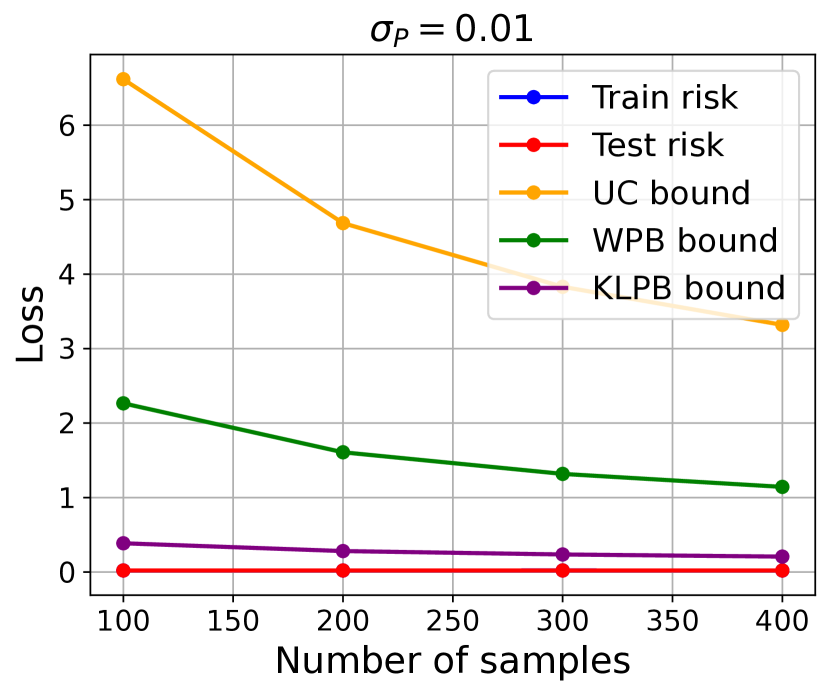
((a)) $\mathbf{\sigma_{P}=10^{-2},\sigma_{Q}=10^{-3}}$

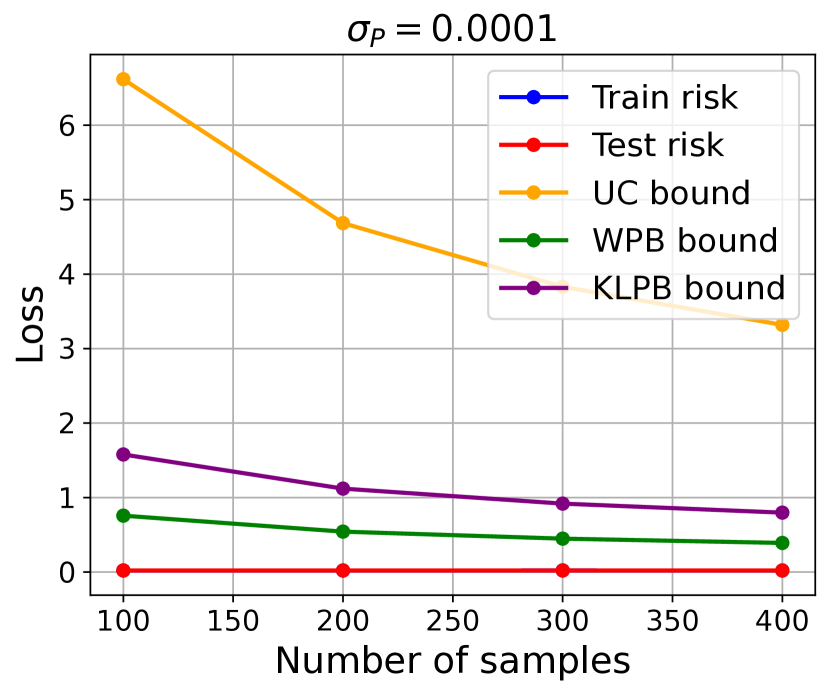
((b)) $\mathbf{\sigma_{P}=10^{-4},\sigma_{Q}=10^{-3}}$

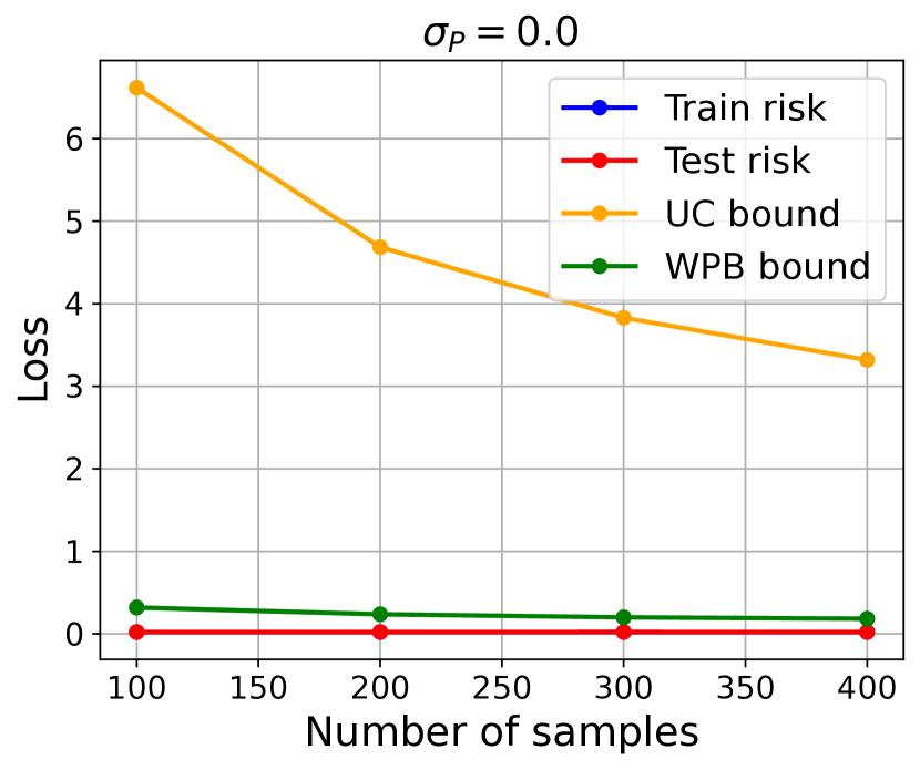
((c)) $\mathbf{\sigma_{P}=\sigma_{Q}=0}$

Figure 2: Linear regression experiment. Note that the the 95% confidence interval is too small to be discernible in the plots, and that blue train risk plot is not visible since it is very close to the test risk.

Appendix D Appendix: Technical Lemmas

Lemma 18.

Let $A\subset\mathbb{R}$ be bounded and non-empty, and let $f:(0,\infty)\to\mathbb{R}$ be continuous and monotone non-decreasing. Then $f(\sup A)=\sup f(A)$, where we defined $\sup A\stackrel{{\scriptstyle\text{def}}}{{=}}\sup_{a\in A}a$, and $\sup f(A)\stackrel{{\scriptstyle\text{def}}}{{=}}\sup_{a\in A}f(a)$; that is, $f(A)$ is the image of the set $A$ under $f$.

Proof.

First notice that $f(\sup A)\geq\sup f(A)$ by monotonicity, because $a\leq\sup A$ for all $a\in A$.

For the other inequality, $f(\sup A)\leq\sup f(A)$ we need to also use continuity: let $\varepsilon>0$; by continuity there exists $\delta>0$ such that for every $a\in A$ such that $a\geq\sup A-\delta$ it holds that $f(a)\geq f(\sup A)-\varepsilon$ (there exists such $a$ by the definition of the supremum). By monotonicity this implies that $\sup f(A)\geq f(\sup A)-\varepsilon$. Since the latter inequality holds for every $\varepsilon>0$, we conclude that $\sup f(A)\geq f(\sup A)$ as required. ∎

Lemma 19 (Wasserstein distance between truncated Gaussian distributions).

Let $X^{(1)}$ and $X^{(2)}$ be the Gaussian random vectors in $\mathbb{R}^{d}$, with distributions $\mathcal{N}(\mu_{1},\Sigma_{1})$, and $\mathcal{N}(\mu_{1},\Sigma_{2})$ respectively. Let $P_{\mymathbb{B}_{r}}:\mathbb{R}^{d}\rightarrow\mymathbb{B}_{r}$ be a projection operator onto the an $r$-radius ball around the origin, $P_{\mymathbb{B}_{r}}(x)\stackrel{{\scriptstyle\text{def}}}{{=}}\operatorname*{argmin}_{x^{\prime}\in\mymathbb{B}_{r}}\left\|x-x^{\prime}\right\|_{2}$, where $\mymathbb{B}_{r}=\left\{x\in\mathbb{R}^{d}:\left\|x\right\|_{2}\leq r\right\}$. Assume that $r\geq\sqrt{\left\|\mu_{j}\right\|_{2}^{2}+\left\|\Sigma_{j}\right\|_{F}^{2}}$ for $j=1,2$. Denote the distribution measures of $X^{(1)}$ and $X^{(2)}$ as $\nu_{1}$ and $\nu_{2}$ respectively. Let $P_{\mymathbb{B}_{r}}\sharp\nu_{1}$ and $P_{\mymathbb{B}_{r}}\sharp\nu_{2}$ be the push-forward measures of $\nu_{1}$ and $\nu_{2}$, respectively, under the operator $P_{\mymathbb{B}_{r}}$. Then

$$W_{1}(P_{\mymathbb{B}_{r}}\sharp\nu_{1},P_{\mymathbb{B}_{r}}\sharp\nu_{2})\leq W_{1}(\nu_{1},\nu_{2})+\sum_{j=1}^{2}\sqrt{\frac{\pi}{2}\left\|\Sigma_{j}\right\|_{2,2}}\operatorname{erfc}\left(\frac{r-\sqrt{\left\|\mu_{j}\right\|_{2}^{2}+\left\|\Sigma_{j}\right\|_{F}^{2}}}{\sqrt{2\left\|\Sigma_{j}\right\|_{2,2}}}\right),$$

where $W_{1}(Q,P)$ denotes the $1^{\mbox{st}}$ order Wasserstein distance with the $L_{2}$ metric.

Proof.

Using the triangle inequality of Wasserstein distances (Clement & Desch, 2008; Thorpe, 2018) twice we get

$$W_{1}(P_{\mymathbb{B}_{r}}\sharp\nu_{1},P_{\mymathbb{B}_{r}}\sharp\nu_{2})\leq W_{1}(P_{\mymathbb{B}_{r}}\sharp\nu_{1},\nu_{1})+W_{1}(\nu_{1},\nu_{2})+W_{1}(\nu_{2},P_{\mymathbb{B}_{r}}\sharp\nu_{2}).$$ (60)

Notice that

$$W_{1}(\nu_{2},P_{\mymathbb{B}_{r}}\sharp\nu_{2}) =\inf_{\gamma\in\Gamma(\nu_{2},P_{\mymathbb{B}_{r}}\sharp\nu_{2})}\int_{\mathbb{R}^{d}\times\mathbb{R}^{d}}\left\|x-x^{\prime}\right\|_{2}\mathrm{d}\gamma(x,x^{\prime})$$ (61)

$$\leq\int_{\mathbb{R}^{d}}\left\|x-P_{\mymathbb{B}_{r}}(x)\right\|_{2}\mathrm{d}\nu_{2}(x)$$

$$\stackrel{{\scriptstyle\textit{\text{(i)}}}}{{=}}\int_{\mathbb{R}^{d}}\left[\left\|x\right\|_{2}-r\right]_{+}\mathrm{d}\nu_{2}(x)$$

$$=\mathbb{E}\left\{\left[\left\|X_{2}\right\|_{2}-r\right]_{+}\right\}$$

$$\stackrel{{\scriptstyle\textit{\text{(ii)}}}}{{=}}\mathbb{E}\left\{\left[V-r\right]_{+}\right\}$$

$$\stackrel{{\scriptstyle\textit{\text{(iii)}}}}{{=}}\int_{t=0}^{\infty}\mathbb{P}\left\{\left[V-r\right]_{+}>t\right\}\mathrm{d}t$$

$$\stackrel{{\scriptstyle\textit{\text{(iv)}}}}{{=}}\int_{t=0}^{\infty}\mathbb{P}\left\{V>r+t\right\}\mathrm{d}t,$$

where in (i) we used the notation $\left[t\right]_{+}\stackrel{{\scriptstyle\text{def}}}{{=}}\begin{cases}t&t>0\\ 0&t\leq 0\end{cases}$ and the equality holds since $P_{\mymathbb{B}_{r}}(x)=x$ for $\left\|x\right\|\leq r$, and $\left\|P_{\mymathbb{B}_{r}}(x)-x\right\|=\left\|x\right\|_{2}-r$ for $\left\|x\right\|>r$ (by the properties of the projection onto the a $L_{2}$ ball). In (ii) we use the definition of the random variable $V\stackrel{{\scriptstyle\text{def}}}{{=}}\left\|X^{(2)}\right\|_{2}$. In (iii) we used the tail sum formula for the expectation. Equality (iv) holds since the corresponding events are equivalent.

Let $Z$ be a standard Gaussian random vector in $\mathbb{R}^{d}$, i.e., $Z\sim\mathcal{N}(\bar{\bm{0}},I)$.

By Wainwright (2019), Thm. 2.26 (one-sided variant) we have that

$$\mathbb{P}\left\{f(Z)-\mathbb{E}\left[f(Z)\right]\geq s\right\}\leq\exp\left(-\frac{s^{2}}{2L^{2}}\right),$$

for any $s\geq 0$ and for any function $f:\mathbb{R}^{d}\to\mathbb{R}$ that is $L$-Lipschitz w.r.t. the $L_{2}$ metric.

In particular, for the function $f(z)\stackrel{{\scriptstyle\text{def}}}{{=}}\left\|\mu_{2}+\Sigma_{2}^{\nicefrac{{1}}{{2}}}z\right\|_{2}$ we have for any $s\geq 0$

$$\mathbb{P}\left\{\left\|\mu_{2}+\Sigma_{2}^{\nicefrac{{1}}{{2}}}Z\right\|_{2}-\mathbb{E}\left[\left\|\mu_{2}+\Sigma_{2}^{\nicefrac{{1}}{{2}}}Z\right\|_{2}\right]\geq s\right\} \leq\exp\left(-\frac{s^{2}}{2\left\|\Sigma_{2}^{\nicefrac{{1}}{{2}}}\right\|_{2,2}^{2}}\right)$$ (62)

$$\stackrel{{\scriptstyle\textit{\text{(i)}}}}{{=}}\exp\left(-\frac{s^{2}}{2\left\|\Sigma_{2}\right\|_{2,2}}\right),$$

since $f$ is Lipschitz with constant $\left\|\Sigma_{2}^{\nicefrac{{1}}{{2}}}\right\|_{2,2}$ where $\left\|\cdot\right\|_{2,2}$ is the operator norm defined by $\left\|A\right\|_{2,2}=\sup_{\left\|x\right\|_{2}=1}\left\|Ax\right\|_{2}$ for any $A\in\mathbb{R}^{d\times d}$. Equality (i) holds since

$$\left\|\Sigma_{2}^{\nicefrac{{1}}{{2}}}\right\|_{2,2}^{2}=\left(\sup_{\left\|x\right\|_{2}=1}\left\|\Sigma_{2}^{\nicefrac{{1}}{{2}}}x\right\|_{2}\right)^{2}=\sup_{\left\|x\right\|_{2}=1}\left\|\Sigma_{2}^{\nicefrac{{1}}{{2}}}x\right\|^{2}_{2}=\sup_{\left\|x\right\|_{2}=1}x^{\top}\Sigma_{2}x=\left\|\Sigma_{2}\right\|_{2,2}.$$

Notice that

$$\mathbb{E}\left[\left\|\mu_{2}+\Sigma_{2}^{\nicefrac{{1}}{{2}}}Z\right\|_{2}\right] =\mathbb{E}\left[\sqrt{\left\|\mu_{2}+\Sigma_{2}^{\nicefrac{{1}}{{2}}}Z\right\|^{2}_{2}}\right]$$

$$\stackrel{{\scriptstyle\textit{\text{(i)}}}}{{\leq}}\sqrt{\mathbb{E}\left\{\left\|\mu_{2}+\Sigma_{2}^{\nicefrac{{1}}{{2}}}Z\right\|^{2}_{2}\right\}}$$

$$=\sqrt{\mathbb{E}\left\{\left(\mu_{2}+\Sigma_{2}^{\nicefrac{{1}}{{2}}}Z\right)^{\top}\left(\mu_{2}+\Sigma_{2}^{\nicefrac{{1}}{{2}}}Z\right)\right\}}$$

$$\stackrel{{\scriptstyle\textit{\text{(ii)}}}}{{=}}\sqrt{\left\|\mu_{2}\right\|_{2}^{2}+\left\|\Sigma_{2}\right\|_{F}^{2}},$$

where (i) is by Jensen’s inequality, and in (ii) we used the fact that $Z\sim\mathcal{N}(\bar{\bm{0}},I)$ and $\left\|\cdot\right\|_{F}$ denotes the Frobenius Norm, defined by $\left\|A\right\|_{F}\stackrel{{\scriptstyle\text{def}}}{{=}}\sqrt{\sum_{i,j}A_{i,j}^{2}}$.

Therefore, using (62), we get

$$\mathbb{P}\left\{\left\|\mu_{2}+\Sigma_{2}^{\nicefrac{{1}}{{2}}}Z\right\|_{2}-\sqrt{\left\|\mu_{2}\right\|_{2}^{2}+\left\|\Sigma_{2}\right\|_{F}^{2}}\geq s\right\}\leq\exp\left(-\frac{s^{2}}{2\left\|\Sigma_{2}\right\|_{2,2}}\right).$$

Note that the random variable $V\stackrel{{\scriptstyle\text{def}}}{{=}}\left\|X^{(2)}\right\|_{2}$ is equal, in distribution, to the random variable $\left\|\mu_{2}+\Sigma_{2}^{\nicefrac{{1}}{{2}}}Z\right\|_{2}$, and therefore we also have for $s\geq 0$ that

$$\mathbb{P}\left\{V-\sqrt{\left\|\mu_{2}\right\|_{2}^{2}+\left\|\Sigma_{2}\right\|_{F}^{2}}\geq s\right\}\leq\exp\left(-\frac{s^{2}}{2\left\|\Sigma_{2}\right\|_{2,2}}\right).$$

For any $t\geq 0$, set $s:=t+r-\sqrt{\left\|\mu_{2}\right\|_{2}^{2}+\left\|\Sigma_{2}\right\|_{F}^{2}}$. Since we assume that $r\geq\sqrt{\left\|\mu_{2}\right\|_{2}^{2}+\left\|\Sigma_{2}\right\|_{F}^{2}}$, we have that $s\geq 0$. Therefore we have

$$\mathbb{P}\left\{V>r+t\right\}\leq\exp\left(-\frac{\left(t+r-\sqrt{\left\|\mu_{2}\right\|_{2}^{2}+\left\|\Sigma_{2}\right\|_{F}^{2}}\right)^{2}}{2\left\|\Sigma_{2}\right\|_{2,2}}\right).$$

Hence, by (61) we have

$$W_{1}(\nu_{2},P_{\mymathbb{B}_{r}}\sharp\nu_{2}) \leq\int_{t=0}^{\infty}\mathbb{P}\left\{V>r+t\right\}\mathrm{d}t$$

$$\leq\int_{t=0}^{\infty}\exp\left(-\frac{\left(t+r-\sqrt{\left\|\mu_{2}\right\|_{2}^{2}+\left\|\Sigma_{2}\right\|_{F}^{2}}\right)^{2}}{2\left\|\Sigma_{2}\right\|_{2,2}}\right)\mathrm{d}t$$

$$=\sqrt{\frac{\pi}{2}\left\|\Sigma_{2}\right\|_{2,2}}\operatorname{erfc}\left(\frac{r-\sqrt{\left\|\mu_{2}\right\|_{2}^{2}+\left\|\Sigma_{2}\right\|_{F}^{2}}}{\sqrt{2\left\|\Sigma_{2}\right\|_{2,2}}}\right).$$

By symmetry we have a similar bound for $W_{1}(P_{\mymathbb{B}_{r}}\sharp\nu_{1},\nu_{1})$. To conclude, using (60) we get

$$W_{1}(P_{\mymathbb{B}_{r}}\sharp\nu_{1},P_{\mymathbb{B}_{r}}\sharp\nu_{2}) \leq W_{1}(P_{\mymathbb{B}_{r}}\sharp\nu_{1},\nu_{1})+W_{1}(\nu_{1},\nu_{2})+W_{1}(\nu_{2},P_{\mymathbb{B}_{r}}\sharp\nu_{2})$$

$$\leq W_{1}(\nu_{1},\nu_{2})+\sum_{j=1}^{2}\sqrt{\frac{\pi}{2}\left\|\Sigma_{j}\right\|_{2,2}}\operatorname{erfc}\left(\frac{r-\sqrt{\left\|\mu_{j}\right\|_{2}^{2}+\left\|\Sigma_{j}\right\|_{F}^{2}}}{\sqrt{2\left\|\Sigma_{j}\right\|_{2,2}}}\right).$$

∎

References

- \NAT@swatrue
- Alquier (2021) Alquier, P. (2021). User-friendly introduction to PAC-Bayes bounds. arXiv preprint arXiv:2110.11216. \NAT@swatrue
- Alquier and Guedj (2018) Alquier, P., and Guedj, B. (2018). Simpler PAC-Bayesian bounds for hostile data. Machine Learning, 107(5), 887–902. \NAT@swatrue
- Aminian et al. (2022) Aminian, G., Bu, Y., Wornell, G., and Rodrigues, M. (2022). Tighter expected generalization error bounds via convexity of information measures. arXiv preprint arXiv:2202.12150. \NAT@swatrue
- Amit and Meir (2018) Amit, R., and Meir, R. (2018). Meta-learning by adjusting priors based on extended PAC-Bayes theory. In International conference on machine learning (ICML) (pp. 205–214). \NAT@swatrue
- Anthony and Bartlett (1999) Anthony, M., and Bartlett, P. L. (1999). Neural network learning: Theoretical foundations (Vol. 9). cambridge university press Cambridge. \NAT@swatrue
- Arjovsky et al. (2017) Arjovsky, M., Chintala, S., and Bottou, L. (2017). Wasserstein generative adversarial networks. In International conference on machine learning (ICML) (pp. 214–223). \NAT@swatrue
- Audibert and Bousquet (2003) Audibert, J.-Y., and Bousquet, O. (2003). PAC-Bayesian generic chaining. In S. Thrun, L. Saul, and B. Schölkopf (Eds.), Advances in neural information processing systems (NeurIPS) (Vol. 16). MIT Press.
- Audibert & Bousquet (2007) Audibert, J.-Y., & Bousquet, O. (2007). Combining PAC-Bayesian and generic chaining bounds. Journal of Machine Learning Research, 8(4).
- Bachmann et al. (2021) Bachmann, G., Moosavi-Dezfooli, S.-M., & Hofmann, T. (2021). Uniform convergence, adversarial spheres and a simple remedy. In International conference on machine learning (ICML) (pp. 490–499).
- Bartlett et al. (2005) Bartlett, P. L., Bousquet, O., & Mendelson, S. (2005). Local Rademacher complexities. The Annals of Statistics, 33(4), 1497–1537.
- Bastani et al. (2021) Bastani, H., Simchi-Levi, D., & Zhu, R. (2021). Meta dynamic pricing: Transfer learning across experiments. Management Science.
- Begin et al. (2016) Begin, L., Germain, P., Laviolette, F., & Roy, J.-F. (2016). PAC-Bayesian bounds based on the rényi divergence. Proceedings of the 19th International Conference on Artificial Intelligence and Statistics (AISTATS).
- Boucheron et al. (2005) Boucheron, S., Bousquet, O., & Lugosi, G. (2005). Theory of classification: A survey of some recent advances. ESAIM: probability and statistics, 9, 323–375.
- Bousquet & Elisseeff (2002) Bousquet, O., & Elisseeff, A. (2002). Stability and generalization. The Journal of Machine Learning Research, 2, 499–526.
- Catoni (2007) Catoni, O. (2007). PAC-Bayesian supervised classification: the thermodynamics of statistical learning. arXiv preprint arXiv:0712.0248.
- Chee & Loustau (2021) Chee, A., & Loustau, S. (2021). Learning with BOT - Bregman and Optimal Transport divergences. hal-03262687v2.
- Chuang et al. (2021) Chuang, C.-Y., Mroueh, Y., Greenewald, K., Torralba, A., & Jegelka, S. (2021). Measuring generalization with optimal transport. Advances in Neural Information Processing Systems, 34, 8294–8306.
- Clement & Desch (2008) Clement, P., & Desch, W. (2008). An elementary proof of the triangle inequality for the Wasserstein metric. Proceedings of the American Mathematical Society, 136(1), 333–339.
- Cuturi (2013) Cuturi, M. (2013). Sinkhorn distances: Lightspeed computation of optimal transport. Advances in neural information processing systems (NeurIPS, 26.
- Dembo & Zeitouni (2009) Dembo, A., & Zeitouni, O. (2009). Ldp for finite dimensional spaces. In Large deviations techniques and applications (pp. 11–70). Springer.
- Donsker & Varadhan (1975) Donsker, M. D., & Varadhan, S. R. S. (1975). Asymptotic evaluation of certain markov process expectations for large time. Comm. Pure Appl. Math..
- Dziugaite & Roy (2017) Dziugaite, G. K., & Roy, D. M. (2017). Computing nonvacuous generalization bounds for deep (stochastic) neural networks with many more parameters than training data. In Conference on uncertainty in artificial intelligence, (UAI).
- Givens & Shortt (1984) Givens, C. R., & Shortt, R. M. (1984). A class of Wasserstein metrics for probability distributions. Michigan Mathematical Journal, 31(2), 231–240.
- Guedj (2019) Guedj, B. (2019). A primer on PAC-Bayesian learning. arXiv preprint arXiv:1901.05353.
- Hou et al. (2022) Hou, S., Kassraie, P., Kratsios, A., Rothfuss, J., & Krause, A. (2022). Instance-dependent generalization bounds via optimal transport. arXiv preprint arXiv:2211.01258.
- Hsu et al. (2012) Hsu, D., Kakade, S., & Zhang, T. (2012). A tail inequality for quadratic forms of subgaussian random vectors. Electronic Communications in Probability, 17, 1–6.
- Jiang et al. (2019) Jiang, Y., Neyshabur, B., Mobahi, H., Krishnan, D., & Bengio, S. (2019). Fantastic generalization measures and where to find them. arXiv preprint arXiv:1912.02178.
- D. Kingma & Ba (2015) Kingma, D., & Ba, J. (2015). Adam: A method for stochastic optimization. In International conference on learning representations (ICLR).
- D. P. Kingma & Welling (2013) Kingma, D. P., & Welling, M. (2013). Auto-encoding variational Bayes. In International conference on learning representations (ICLR).
- Koltchinskii & Panchenko (2004) Koltchinskii, V., & Panchenko, D. (2004). Rademacher processes and bounding the risk of function learning. arXiv preprint math/0405338.
- Lever et al. (2013) Lever, G., Laviolette, F., & Shawe-Taylor, J. (2013). Tighter PAC-Bayes bounds through distribution-dependent priors. Theor. Comput. Sci., 473(Feb), 4–28.
- Livni & Moran (2020) Livni, R., & Moran, S. (2020). A limitation of the PAC-Bayes framework. Advances in Neural Information Processing Systems (NeurIPS), 33, 20543–20553.
- Lopez & Jog (2018) Lopez, A. T., & Jog, V. (2018). Generalization error bounds using wasserstein distances. In 2018 ieee information theory workshop (ITW) (pp. 1–5).
- Lugosi (2002) Lugosi, G. (2002). Pattern classification and learning theory. In Principles of nonparametric learning (pp. 1–56). Springer.
- Mardia et al. (2019) Mardia, J., Jiao, J., Tánczos, E., Nowak, R. D., & Weissman, T. (2019, 11). Concentration inequalities for the empirical distribution of discrete distributions: beyond the method of types. Information and Inference: A Journal of the IMA, 9(4), 813-850.
- Maurer (2004) Maurer, A. (2004). A note on the PAC Bayesian theorem. CoRR abs/cs/0411099.
- McAllester (1998) McAllester, D. (1998). Some PAC-Bayesian theorems. Conference on Learning Theory (COLT).
- McAllester (2003) McAllester, D. (2003). Simplified PAC-Bayesian margin bounds. Conference on Learning Theory (COLT).
- Miyaguchi (2019) Miyaguchi, K. (2019). PAC-Bayesian transportation bound. arXiv preprint arXiv:1905.13435.
- Müller (1997) Müller, A. (1997). Stochastic orders generated by integrals: a unified study. Advances in Applied probability, 29(2), 414–428.
- Nagarajan & Kolter (2019a) Nagarajan, V., & Kolter, J. Z. (2019a). Deterministic PAC-Bayesian generalization bounds for deep networks via generalizing noise-resilience. arXiv preprint arXiv:1905.13344.
- Nagarajan & Kolter (2019b) Nagarajan, V., & Kolter, J. Z. (2019b). Uniform convergence may be unable to explain generalization in deep learning. Advances in Neural Information Processing Systems (NeurIPS), 32.
- Neu & Lugosi (2022) Neu, G., & Lugosi, G. (2022). Generalization bounds via convex analysis. arXiv preprint arXiv:2202.04985.
- Neyshabur et al. (2017) Neyshabur, B., Bhojanapalli, S., McAllester, D., & Srebro, N. (2017). Exploring generalization in deep learning. Advances in Neural Information Processing Systems (NeurIPS), 30.
- Neyshabur et al. (2015) Neyshabur, B., Tomioka, R., & Srebro, N. (2015). Norm-based capacity control in neural networks. In Conference on learning theory (pp. 1376–1401).
- Ohnishi & Honorio (2021) Ohnishi, Y., & Honorio, J. (2021). Novel change of measure inequalities with applications to PAC-Bayesian bounds and monte carlo estimation. In International conference on artificial intelligence and statistics (pp. 1711–1719).
- Paszke et al. (2019) Paszke, A., Gross, S., Massa, F., Lerer, A., Bradbury, J., Chanan, G., … others (2019). Pytorch: An imperative style, high-performance deep learning library. Advances in Neural Information Processing Systems (NeurIPS), 32.
- Picard-Weibel & Guedj (2022) Picard-Weibel, A., & Guedj, B. (2022). On change of measure inequalities for -divergences. arXiv preprint arXiv:2202.05568.
- Rivasplata et al. (2020) Rivasplata, O., Kuzborskij, I., Szepesvári, C., & Shawe-Taylor, J. (2020). PAC-Bayes analysis beyond the usual bounds. Advances in Neural Information Processing Systems (NeurIPS), 33, 16833–16845.
- Rodríguez Gálvez et al. (2021) Rodríguez Gálvez, B., Bassi, G., Thobaben, R., & Skoglund, M. (2021). Tighter expected generalization error bounds via Wasserstein distance. Advances in Neural Information Processing Systems (NeurIPS), 34.
- Seeger (2002) Seeger, M. (2002). PAC-Bayesian generalisation bounds for gaussian processes. Journal of Machine Learning Research, 3:233-269.
- Seldin & Tishby (2010) Seldin, Y., & Tishby, N. (2010). PAC-Bayesian analysis of co-clustering and beyond. JMLR 2010.
- Shalev-Shwartz & Ben-David (2014) Shalev-Shwartz, S., & Ben-David, S. (2014). Understanding machine learning: From theory to algorithms. Cambridge University Press.
- Shawe-Taylor & Williamson (1997) Shawe-Taylor, J., & Williamson, R. C. (1997). A PAC analysis of a Bayesian estimator. Proceedings of the International Conference on Computational Learning Theory (COLT).
- Sriperumbudur et al. (2009) Sriperumbudur, B. K., Fukumizu, K., Gretton, A., Schölkopf, B., & Lanckriet, G. R. (2009). On integral probability metrics, -divergences and binary classification. arXiv preprint arXiv:0901.2698.
- Sriperumbudur et al. (2012) Sriperumbudur, B. K., Fukumizu, K., Gretton, A., Schölkopf, B., & Lanckriet, G. R. (2012). On the empirical estimation of integral probability metrics. Electronic Journal of Statistics, 6, 1550–1599.
- Talagrand (1994) Talagrand, M. (1994). Sharper bounds for gaussian and empirical processes. The Annals of Probability, 28–76.
- Thorpe (2018) Thorpe, M. (2018). Introduction to optimal transport. Notes of Course at University of Cambridge..
- Vapnik (1999) Vapnik, V. (1999). The nature of statistical learning theory. Springer science & business media.
- Vapnik & Chervonenkis (2015) Vapnik, V., & Chervonenkis, A. Y. (2015). On the uniform convergence of relative frequencies of events to their probabilities. In Measures of complexity (pp. 11–30). Springer.
- Villani (2006) Villani, C. (2006). Optimal transport: old and new. Springer Science and Business Media.
- Wainwright (2019) Wainwright, M. J. (2019). High-dimensional statistics: A non-asymptotic viewpoint (Vol. 48). Cambridge University Press.
- Wang et al. (2019) Wang, H., Diaz, M., Santos Filho, J. C. S., & Calmon, F. P. (2019). An information-theoretic view of generalization via Wasserstein distance. In 2019 IEEE international symposium on information theory (ISIT) (pp. 577–581).
- Weed & Bach (2017) Weed, J., & Bach, F. (2017). Sharp asymptotic and finite-sample rates of convergence of empirical measures in Wasserstein distance. Bernoulli 25 (4A), 2620-2648.
- Wei & Ma (2019) Wei, C., & Ma, T. (2019). Data-dependent sample complexity of deep neural networks via lipschitz augmentation. arXiv preprint arXiv:1905.03684.
- Xu & Mannor (2012) Xu, H., & Mannor, S. (2012). Robustness and generalization. Machine learning, 86(3), 391–423.
- Yang et al. (2019) Yang, J., Sun, S., & Roy, D. M. (2019). Fast-rate PAC-Bayes generalization bounds via shifted Rademacher processes. arXiv preprint arXiv:1908.07585.
- C. Zhang et al. (2017) Zhang, C., Bengio, S., Hardt, M., Recht, B., & Vinyals, O. (2017). Understanding deep learning requires rethinking generalization. International Conference on Learning Representations (ICLR).
- J. Zhang et al. (2021) Zhang, J., Liu, T., & Tao, D. (2021). An optimal transport analysis on generalization in deep learning. IEEE Transactions on Neural Networks and Learning Systems.