Quadratic growth during the COVID-19 pandemic: merging hotspots and reinfections

Abstract

The existence of an exponential growth phase during early stages of a pandemic is often taken for granted. However, for the 2019 novel coronavirus epidemic, the early exponential phase lasted only for about six days, while the quadratic growth prevailed for forty days until it spread to other countries and continued, again quadratically, but with a larger coefficient. Here we show that this rapid phase is followed by a subsequent slow-down where the coefficient is reduced to almost the original value at the outbreak. This can be explained by the merging of previously disconnected sites that occurred after the disease jumped (nonlocally) to a relatively small number of separated sites. Subsequent variations in the slope with continued growth can qualitatively be explained as a result of reinfections and changes in their rate. We demonstrate that the observed behavior can be described by a standard epidemiological model with spatial extent and reinfections included. Time-dependent changes in the spatial diffusion coefficient can also model corresponding variations in the slope.

Keywords: quadratic growth, SIR model, front propagation

1 Introduction

Soon after the news about the 2019 novel coronavirus epidemic emerged, people in Europe followed the increasing case numbers with concern [1, 2, 3, 4, 5, 6, 7, 8, 9, 10, 11, 12]. The first deaths occurred on January 20, and, for a long time, the ratio of the number of deaths to that of cases was around 0.02. Even today (December 2022), with $6.7\times 10^{6}$ deaths and $6.6\times 10^{8}$ cases worldwide, the ratio is still about 0.01.

It soon became clear that the number of cases increased subexponentially [13, 14, 15, 16, 17, 18, 19, 20]. This was called peripheral growth [13], which means that the rate of increase of the number of cases or deaths is proportion to the length $\ell$ of the periphery of a patch on a map containing the population with the disease. If it is just a circular patch of radius $r$, the circumference is $\ell=2\pi r$ and the number of cases is $N_{i}=n_{i}\pi r^{2}$, where $n_{i}$ is the density of cases ($i={\rm C}$) or deaths ($i={\rm D}$) per unit area. The rate of increase of $N_{i}$ is then

$$\frac{\,{\rm d}N_{i}}{\,{\rm d}t}=\alpha\ell=2\alpha(\pi N_{i}/n_{i})^{1/2},\quad i={\rm C},{\rm D}$$ (1)

for “cases” and “deaths” with the solution

$$N_{i}^{1/2}=N_{i0}^{1/2}+(t-t_{0})/\tau,$$ (2)

where $N_{i0}=N_{i}(t_{0})$ is the initial condition at $t=t_{0}$ and $1/\tau=\alpha(\pi/n_{i})^{1/2}$ is the slope. Thus, we expect a quadratic growth where $N_{i}^{1/2}$ versus $t$ increases linearly or piecewise linearly with $t$. This was clearly seen in the original study in Ref. [13]. Subsequent work confirmed the existence of algebraic growth, although the exponent was sometimes found to deviate from 2. This could be related to growth on a fractal [14]. In Figure 1, we present an updated plot of the square of the number of deaths, $N_{\rm D}^{1/2}$, versus $t$. We identify five different slopes, A–E, whose values and their reciprocal values are given in Table LABEL:TAB.

Of particular importance is the fact that, at some point, the quadratic growth sped up; see Figure 1 at $t\approx 50\,{\rm days}$ after January 20, 2020, or Figure 2 of Ref. [13]. This was possible to model through the emergence of multiple nucleation sites from where the disease spread. This meant that the coefficient $\alpha$ should be replaced by $\alpha\to\alpha_{1}+\alpha_{2}+...+\alpha_{M}$, depending on the number $M$ of sites, increasing thereby the slope of $N_{i}^{1/2}$.

It was already anticipated in Ref. [21] that the subsequent decrease of the growth of the number of cases and deaths could be associated with the merging of independent sites from which separated fronts continue to expand after an initial period of quadratic increase in the number of cases or deaths. The details of this process were not, however, explored in detail. This is the purpose of the present paper. We begin by discussing the spatially extended version of the standard $SIR$ model [22], where $S$ stands for the number of susceptible individuals, $I$ for the number of infectious individuals, and $R$ for the number of recovered, deceased, or immune individuals.

2 The spatially extended $SIR$ model

In epidemics, the $SIR$ model and its extensions are an important corner stone in the theory of epidemics. The extension to including a diffusion operator, i.e., $\kappa\nabla^{2}$, where $\kappa$ is the diffusivity, is important when complete mixing among the population can no longer be assumed. Their inclusion has dramatic consequences for the evolution of the total number of cases or deaths. In the following, we discuss the consequences in detail. We begin by outlining the essence of the $SIR$ model

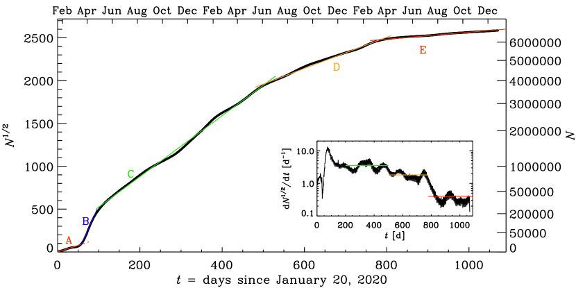
Figure 1: Square root of the number $N$ of deaths, which is regarded as a proxy of the number of infected that is more reliable than the reported number of SARS-CoV-2. Note the piecewise linear growth in $N^{1/2}$, corresponding to a piecewise quadratic growth. The line segments A–E are described in the text.

Table 1: Parameters of the five intervals of Figure 1.

Interval $1/\tau$ [$\,{\rm d}^{-1}$] $\tau$ [$\,{\rm d}$] A 1.54 0.65 B 10.7 0.09 C 3.55 0.28 D 1.82 0.55 E 0.41 2.5

2.1 Formulation of the model

In its original form, the $SIR$ model assumes perfect mixing and therefore spatial homogeneity. Therefore, spatial gradients are absent and $\kappa=0$. The basic equations, with $\kappa\neq 0$, are

$${\partial S\over\partial t}=-\lambda SI+\gamma^{\prime}R,$$ (3)

$${\partial I\over\partial t}=\lambda SI-\mu I+\gamma R+\kappa\nabla^{2}I,$$ (4)

$${\partial R\over\partial t}=\mu I-(\gamma+\gamma^{\prime})R,$$ (5)

where $\lambda$ is the reproduction rate, $\mu$ is the rate of recovery, while $\gamma$ and $\gamma^{\prime}$ characterize the rates of reinfection either directly via $I$ or by producing susceptible first, respectively. The latter case ($\gamma=0$ with $\gamma^{\prime}\neq 0$) is also known as the SIRS model. Modeling reinfections through $\gamma^{\prime}\neq 0$ instead of $\gamma\neq 0$ can result in a slight reduction of $\langle I\rangle$, especially when $\mu$ is large.

Note that the model preserves the total population, i.e., $S+I+R={\rm const}\equiv S_{0}$ when $\kappa=0$ and $\langle S+I+R\rangle={\rm const}\equiv S_{0}$ when $\kappa\neq 0$, where angle brackets denote an average over the population. Here, $S_{0}$ is the initial population. Therefore, only two of the three equations need to be solved.

In essence, the standard version of the model with $\gamma=\gamma^{\prime}=0$ describes the increase of cases based on the current number of susceptible individuals. Once this number begins to be depleted, it can only decrease, although it can still increase in neighboring locations, where the number of cases may still be smaller. This leads to spatial spreading of the disease and thereby ultimately to an increase in the total number of cases. Thus, the $SIR$ model with spatial extend is capable of describing the increase of cases and deaths. It remains unclear, however, whether the spatial increase corresponds to a complete or only partially space-filling increase in the number of cases over the surface of the Earth. Given that the current number of cases now reaches a significant fraction of the total population on Earth, it may indeed be plausible that soon every single individual on Earth is and was susceptible to the disease.

We solve Equations (3) and (4) in a two-dimensional Cartesian domain with coordinates $\bm{x}=(x,y)$ and periodic boundary conditions. We characterize the domain size $L$ by the smallest wavenumber $k=2\pi/L$ that fits into the domain. We use the Pencil Code, a publicly available time stepping code for solving partial differential equations on massively parallel computers [23]. Spatial derivatives are computed from a sixth-order finite difference formula and a third order Runge–Kutta time stepping scheme is employed. As in Ref. [13], we use $4096^{2}$ mesh points and run the model for about 1200 time units. (During that time interval, the periodicity of the domain did not yet play any role, because the disease did not reach the boundary.) The $SIR$ model is implemented in the current version, and also the relevant input parameter files are publicly available [21].

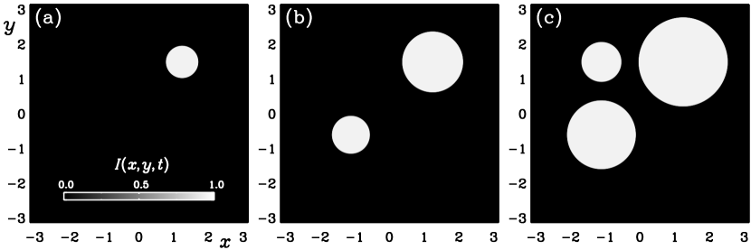
Figure 2: $I(x,y,t)$ for $\mu=\gamma=\gamma^{\prime}=0$ with $\kappa=10^{-6}$ and normalized times (a) $\lambda t=300$, (b) $500$, and (c) $700$.

We define nondimensional space and time coordinates as $\tilde{\bm{x}}=k\bm{x}$ and $\tilde{t}=\lambda t$, respectively. Furthermore, $\tilde{\mu}=\mu/\lambda$, $\tilde{\gamma}=\gamma/\lambda$, $\tilde{\gamma}^{\prime}=\gamma^{\prime}/\lambda$, and $\tilde{\kappa}=\kappa k^{2}/\lambda$ are the only nondimensional input parameters that will be varied. The population is normalized by $S_{0}$, so we can define $\tilde{S}=S/S_{0}$, $\tilde{I}=I/S_{0}$, and $\tilde{R}=R/S_{0}$ as the fractional (nondimensional) population densities. We then have $\langle\tilde{S}+\tilde{I}+\tilde{R}\rangle=1$ at all times. The tildes will from now on be dropped. In practice, we keep $\lambda=1$ and adopt for the domain size $L=2\pi$, so $k=1$. For clarity, we often retain the factor $\lambda$ in front of the time to remind the reader of the normalization. Similarly, we often keep the normalizations of $\mu$, $\gamma$, and $\gamma^{\prime}$ and quote for the diffusivity the combination $\kappa k^{2}/\lambda$ instead of just $\kappa$.

As initial condition, we assume $S=1$ and $I=0$, except for those mesh points, where we initialize $I=I_{1}$ on one isolated mesh point and $I=I_{2}$ on eight others. We refer to them as “hotspot”.

2.2 Emergence of hotspots

The main result of Ref. [13] was that each hotspot, once it reaches locally its saturation value, continues to grow only by spreading on the periphery. This peripheral growth is always quadratic. However, once a new hotspot emerges, the coefficient in the growth law increases. Figures 2 and 3 provide an example of this. At $\lambda t=300$, there is just one patch and the derivative of $\langle I\rangle^{1/2}$ with respect to $\lambda t$ is about $6\times 10^{-4}$. When the next patch is established, the derivative becomes about $8\times 10^{-4}$, and after the third, the derivative becomes about $10^{-3}$. Thus, it seems that with each patch, the derivative increases by about $2\times 10^{-4}$. However, there is an offset by about $4\times 10^{-4}$ for the first one. There is also a strong spike early on at $\lambda t\approx 150$. The existence of these two features suggests that there is an additional contribution to the overall growth that is independent of the number of patches. These aspects are obviously not captured by the simple peripheral growth model discussed in the introduction. Interestingly, piecewise constant time derivatives have previously been seen in a system where two populations compete against each other and one of the two eventually disappears [24]. In that case, it was the area that decreased linearly with time and there was no offset as in the present case.

Figure 3: Time series for a simulation with 3 hotspots of different strengths. Note that $N^{1/2}\propto\langle I\rangle^{1/2}$ grows in a piecewise linear fashion with time $t$. The inset shows the normalized derivative $\,{\rm d}\langle I\rangle^{1/2}/\,{\rm d}(\lambda t)$. The horizontal dotted lines mark the values $6\times 10^{-4}$, $8\times 10^{-4}$, and $10^{-3}$.

2.3 Merging of patches

The main purpose of the present study is to explain what happens when different hotspots begin to merge at some moment. Figure 4 shows an example with initially nine separated hotspots. In this model, $\mu=\gamma=\gamma^{\prime}=0$, so there is no recovery and no reinfections. As before, the diffusivity is $\kappa k^{2}/\lambda=10^{-6}$. By the time $\lambda t=300$, all patches have begun to merge, so the total length of the periphery has decreased, and therefore also the slope of growth has decreased; see Figure 5. Quantitatively, the slope decreased from about $1.7\times 10^{-3}$ to about $6\times 10^{-4}$, which is the same value that was found for a single patch.

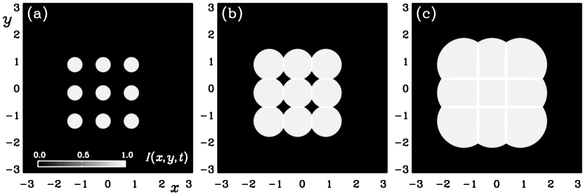
Figure 4: Simulation with 9 hotspots that later merge and overlap. The local distribution of $I(x,y,t)$ is shown in the $xy$ plane for three values of $t$ ($\lambda t=150$, 300, and 500). The length of the circumference determines the speed of growth. When several hotspots merge, the circumference shortens and the growth slows down. Here, $\mu=\gamma=\gamma^{\prime}=0$ and $\kappa k^{2}/\lambda=10^{-6}$.

We argue that the phenomenon of merging models qualitatively the decrease of the slope in Figure 1 at $t\approx 100\,{\rm days}$ after January 20, 2020. This implies that from that moment onward (beginning of May 2020), the disease has begun to affect the entire world and the speed of spreading was limited only by the containment efforts that took place everywhere.

Figure 5: Time series for simulation with 9 hotspots that later overlap. Note that $N^{1/2}\propto\langle I\rangle^{1/2}$ grows linearly with time $t$, which shows that $N\propto t^{2}$. The inset shows the early exponential growth phase.

What the original $SIR$ model was not taking into account is the concept of reinfection ($\gamma\neq 0$ or $\gamma^{\prime}\neq 0$), i.e., the fact that infected people can, after a certain period of time, be infected again. This means that we must account for a term that describes the decrease of reinfected individuals, which leads to a source in the number of people that can be infected. The purpose of the following is to explore in more detail the effect of the sustainment of cases by the phenomenon of reinfection.

2.4 Models with reinfection

Next, we study models where the effect of reinfections is included, i.e., $\gamma\neq 0$. In Figures 6 and 7, we consider models with different values of $\gamma$ and compare with cases where $\gamma^{\prime}\neq 0$. We only study cases with $\mu\neq 0$, because otherwise there are no recoveries ($R=0$) and hence also no reinfections are possible. We begin by considering here a relatively small value of $\mu/\lambda=5\times 10^{-3}$ and then also take a larger one of 0.1; see Figure 10 of Ref. [13] for other experiments with those values of $\mu$. When $\mu$ is small, there is a slow decline in the cores of each of patch; see Figure 6(a). When there are reinfections ($\gamma\neq 0$ or $\gamma^{\prime}\neq 0$), the cores are being prevented from depleting all the way to zero and thus level off at a finite value of a about 0.95 for $\gamma/\lambda=0.1$; see Figure 6(b).

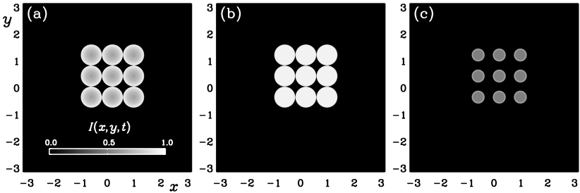
Figure 6: Similar to Figure 4, but for models with (a) $\mu/\lambda=5\times 10^{-3}$ and $\gamma=0$, (b) $\mu/\lambda=5\times 10^{-3}$ and $\gamma/\lambda=0.1$, and (c) $\mu/\lambda=0.1$ and $\gamma/\lambda=0.1$, all at $\lambda t=500$. They illustrate that reinfections ($\gamma/\lambda=0.1$) lead to an increase (b), but that increase diminishes significantly when the rate of recovery is increased from $\mu/\lambda=5\times 10^{-3}$ to 0.1 (c).

We also studied a more extreme case where we $\mu/\lambda=0.1$. In that case, even for $\gamma/\lambda=0.1$, the level of infections remains at a residual level of about $0.55$. This continued growth models the behavior seen at later times in Figure 1.

Figure 7 shows that the two models (b) and (c) with $\gamma/\lambda=0.1$ (or $\gamma^{\prime}/\lambda=0.1$ for the dashed lines) have nearly the same spreading speed. This has to do with the fact that the spreading speed is primarily determined by the diffusivity, as will be addressed next. The larger rate of recovery in (c) is responsible for the downward shift compared with (b).

Figure 7: Similar to Figure 5, but for the cases (a)–(c) of Figure 6. The fat dashed red (b) and blue (c) lines denote cases where $\gamma=0$ and $\gamma^{\prime}/\lambda=0.1$ has been chosen. They show that the choice of the specific reinfection model has only a small effect and leads to a mild decrease of $\langle I\rangle^{1/2}$ when $\mu/\lambda=0.1$ (c).

2.5 Diffusion determines expansion speed

As already emphasized in Ref. [13], and as expected from the theory of epidemic front propagation [25, 26], the value of $\kappa$ determines the speed of expansion. This is shown in Figure 8, where we compare models with finite rates of recovery ($\mu/\lambda=0.1$) and reinfection by the SIRS model ($\gamma^{\prime}/\lambda=0.1$), and three different diffusivities ($\kappa k^{2}/\lambda=10^{-6}$, $2\times 10^{-6}$, and $5\times 10^{-6}$), all at $\lambda t=500$. We clearly see that the speed increases with increasing values of $\kappa$ and that the patches are correspondingly larger after the same amount of time. The corresponding time traces for those three values of $\kappa$ are compared in Figure 9. Here we see that the slopes increase with increasing values of $\kappa$, but decrease again once the patches begin to merge.

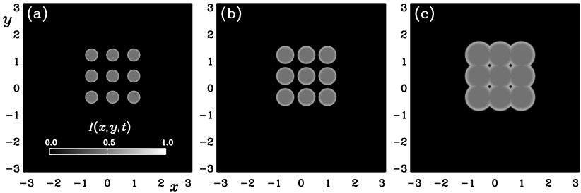
Figure 8: Similar to Figure 4, but for models with $\mu/\lambda=0.1$, $\gamma=0$, and $\gamma^{\prime}/\lambda=0.1$ with (a) $\kappa k^{2}/\lambda=10^{-6}$, (b) $2\times 10^{-6}$, and (c) $5\times 10^{-6}$, all at $\lambda t=500$. Note that a larger diffusivity leads to larger patches in a fixed amount of time. For the largest diffusivity $\kappa k^{2}/\lambda=5\times 10^{-6}$ (c), the patches do already overlap at $\lambda t=500$.

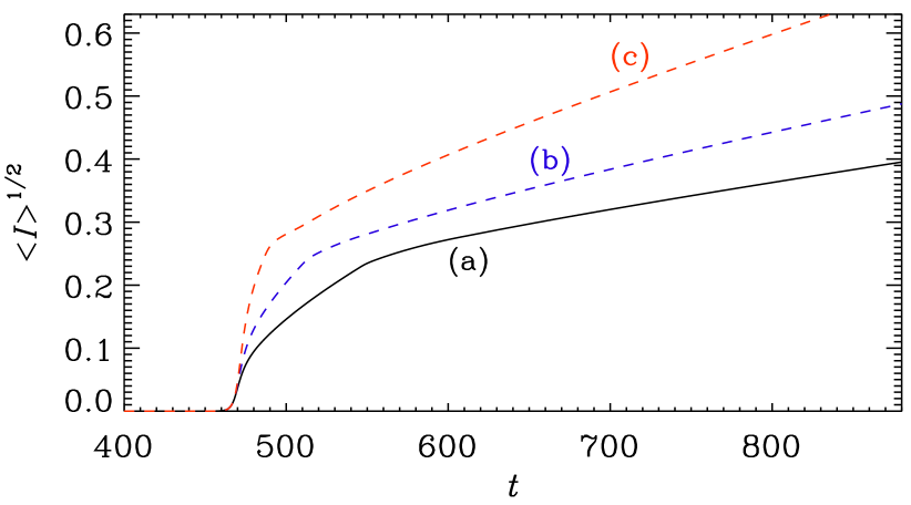
Figure 9: Similar to Figure 5, but for the cases (a)–(c) of Figure 8. Note that the slopes increase with increasing values of $\kappa$, but decrease again once the patches begin to merge, which is the case at $\lambda t\approx 490$ (a), 512 (b), and 550 (c) for the three values of $\kappa$. Note also that panel (a) corresponds to Figure 7(c), where reinfection is modeled by $\gamma/\lambda=0.1$ instead of $\gamma^{\prime}/\lambda=0.1$ in the present case.

Figure 8(a), where $\gamma^{\prime}/\lambda=0.1$ and $\gamma=0$, also shows that the choice of the specific reinfection model is not important for the final result. This can be seen by comparing with Figure 7(c), which is the same model, except that here $\gamma^{\prime}=0$ and $\gamma/\lambda=0.1$. Note that the corresponding time traces were already compared in Figure 6; see the solid and dashed blue lines for case (c).

2.6 Decreases in the slope

Given that the expansion speed depends on the value of $\kappa$, one must expect that a time-dependent decrease of $\kappa$ should lead to a decrease in the spreading speed. This is shown in Figure 10(a), where we used the model of Figure 6(c) and restarted it at $\lambda t=600$ with smaller diffusivities.

Likewise, a decrease in the reinfection rate should also lead to a decrease in the speed of spreading. It turns out, however, that a sudden decrease in the reinfection rate, for example from $\gamma^{\prime}/\lambda=0.1$ to 0.05, has immediately a rather noticeable effect on $\langle I\rangle^{1/2}$. It is therefore desirable to let $\gamma^{\prime}$ decrease in a smooth fashion. Here we have chosen a modulation of the form

$$\gamma^{\prime}=\gamma_{0}^{\prime}\,\Theta(t;\;t_{1},t_{2}),$$ (6)

where

$$\Theta(t)=\max\left\{0,\;1-\left[\frac{\max(0,\;t-t_{1})}{t_{2}-t_{1}}\right]^{2}\right\}^{2}$$ (7)

is a function that goes smoothly from unity to zero between $t=t_{1}$ and $t=t_{2}$. The additional arguments $t_{1}$ and $t_{2}$ have here been suppressed for brevity.

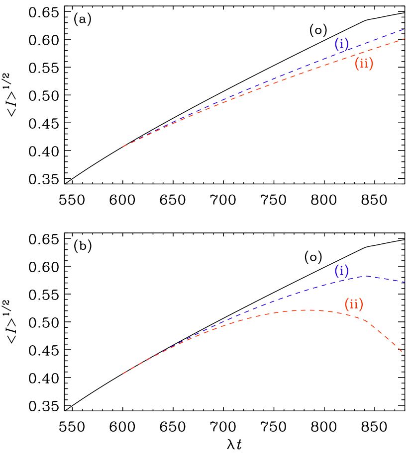
Figure 10: Decreasing slopes from (a) decreasing values of $\kappa$ and (b) decreasing reinfection rates $\gamma^{\prime}$. The reference run (o) is the same as (c) in Figures 8 and 9 with $\mu/\lambda=\gamma^{\prime}/\lambda=0.1$, $\gamma=0$, and $\kappa k^{2}/\lambda=5\times 10^{-6}$. In both cases we restart at $\lambda t=600$. In (a), we use (i) $\kappa k^{2}/\lambda=2\times 10^{-6}$ and (ii) $10^{-6}$, while in (b) we use Equations (6) and (7) and (i) $\lambda t_{2}=1000$ and (ii) $\lambda t_{2}=1200$.

In Figure 10(b), we show cases with $\lambda t_{2}=1200$ (i) and $\lambda t_{2}=1000$ (ii), restarting again at $\lambda t_{1}=600$. The results are promising and can serve to explain the decreases in the slope seen in Figure 1.

3 Conclusions

The present work has shown that the number of infected people will not increase exponentially, as expected for a well mixed model without spatial extend, but that it can increase instead quadratically and can be both slower, if the local number of infected people is already exhausted, and faster, if the number of susceptible people can still increase in neighboring locations.

Obviously, the local number of cases cannot increase indefinitely, but it can increase owing to the fact that the people in neighboring locations can be infected and infected people can even be reinfected. In the present work, we have studied in more detail the effect of reinfections, which is especially important in cases when most of the population has already been infected. It turns out that a decrease in the total number of infections worldwide can be explained by the merging of originally separated spreading centers. In the case of SARS-CoV2, this happened at more or less the same time (around $t\approx 50\,{\rm days}$ in Figure 1) for all the different spreading centers on the Earth.

Subsequent variations in the number of cases and deaths can be explained by variations in the reinfection rate. This has been demonstrated by decreasing $\gamma^{\prime}$ after a certain time, and it led to a decrease in the spreading speed. Similar results can also be reproduced by decreasing the diffusivity at some time. This would model a tightening of the control interventions and containment regulations, but this is unlikely to explain the actual decrease in the slope seen in Figure 1. Instead, a gradual decrease in the reinfection rate appears to be the more plausible phenomenon causing the monotonic decrease in the slope see in Figure 1.

It is worth reflecting again on the meaning of patches. It is not evident that the spreading of the disease can really be described through patches. However, the ability of our model in explaining quadratic growth is rather generic and we may therefore be tempted to search more thoroughly for an appropriate interpretation.

In this context, it is important to emphasize that quadratic growth is not just an unspecified realization of governmental containment efforts and control interventions of the disease, as was originally speculated [15, 27]. Instead, containment efforts may really mean that much of the population was really excluded from the original spreading centers, and that the disease is also so contagious that perfect containment was never possible, so that there was always some leakage out of the patches or hotspots. Within each patch, on the other hand, the level of infections is always essentially saturated, which also explains why the early exponential growth of the disease was so short. This is also seen in our present simulations see; see the inset of Figure 5.

In conclusion, our findings and interpretations of quadratic growth are not so much a statement that we can predict a disease outcome, and certainly not easily at the national level, but it is rather a way of charactering the nature of SARS-CoV2 as an extremely contagious disease that will easily spread locally to the maximum possible level and can then be characterized as peripheral diffusive growth for each of the patches. By now, SARS-CoV2 has almost affected the entire population, and yet, the case numbers keep slowly increasing; see Table LABEL:TAB. Within our $SIR$ model with spatial extent, this can be described by including reinfections in our equations. The level of reinfections can easily be fluctuating because of seasonal and other effects, which explains the long period of growth with piecewise different (and mostly decreasing) slopes.

Code and data availability statement

The source code used for the simulations of this study, the Pencil Code [23], is freely available on https://github.com/pencil-code/, with datasets on Zenodo, doi:10.5281/zenodo.4016941.

ORCID

Axel Brandenburg:
http://orcid.org/0000-0002-7304-021X

References

References

- [1] Backer J A, Klinkenberg D and Wallinga J 2020 Eurosurveillance 25 10–15 ISSN 1025-496X
- [2] Zhou T, Liu Q, Yang Z, Liao J, Yang K, Bai W, Lu X and Zhang W 2020 J. Evidence Based Medicine 13 3–7 ISSN 1756-5383
- [3] Singer H M 2020 Phys. Biol. 17 ISSN 1478-3967
- [4] Wu K, Darcet D, Wang Q and Sornette D 2020 Nonlin. Dynam. 101 1561–1581 ISSN 0924-090X
- [5] Britton T, Ball F and Trapman P 2020 Science 369 846+ ISSN 0036-8075
- [6] Prasse B, Achterberg M A, Ma L and Van Mieghem P 2020 Appl. Network Sci. 5
- [7] Chen Y, Cheng J, Jiang Y and Liu K 2020 J. Inverse and Ill-posed Problems 28 243–250 ISSN 0928-0219
- [8] Wu J T, Leung K and Leung G M 2020 Lancet 395 689–697 ISSN 0140-6736
- [9] Britton T 2020 Statistica Neerlandica 74 222–241 ISSN 0039-0402
- [10] Wang F S and Zhang C 2020 Lancet 395 391–393 ISSN 0140-6736
- [11] Tang B, Bragazzi N L, Li Q, Tang S, Xiao Y and Wu J 2020 Infectious Disease Modelling 5 248–255
- [12] Roosa K, Lee Y, Luo R, Kirpich A, Rothenberg R, Hyman J M, Yan P and Chowell G 2020 Infectious Disease Modelling 5 256–263
- [13] Brandenburg A 2020 Infectious Disease Modelling 5 681–690
- [14] Ziff A L and Ziff R M 2020 Int. J. Educational Excellence 6 43–69 ISSN 2373-5929
- [15] Maier B F and Brockmann D 2020 Science 368 742+ ISSN 0036-8075
- [16] Bod’ova K and Kollar R 2020 Phys. Biol. 17 ISSN 1478-3967
- [17] Radicchi F and Bianconi G 2020 Phys. Rev. E 102 ISSN 2470-0045
- [18] Blanco N, Stafford K A, Lavoie M C, Brandenburg A, Gorna M W and Merski M 2021 Epidemiology and Infection 149 ISSN 0950-2688
- [19] Triambak S, Mahapatra D P, Mallick N and Sahoo R 2021 Epidemics 37 ISSN 1755-4365
- [20] Rast M P 2022 Phys. Rev. E 105 ISSN 2470-0045
- [21] Brandenburg A 2020 Datasets for Piecewise quadratic growth during the 2019 novel coronavirus epidemic, doi:10.5281/zenodo.4016941 (v2020.09.07)
- [22] Kermack W O and McKendrick A G 1927 Proc. Roy. Soc. Lond. Ser. A 115 700–721
- [23] Pencil Code Collaboration, Brandenburg A, Johansen A, Bourdin P, Dobler W, Lyra W, Rheinhardt M, Bingert S, Haugen N, Mee A, Gent F, Babkovskaia N, Yang C C, Heinemann T, Dintrans B, Mitra D, Candelaresi S, Warnecke J, Käpylä P, Schreiber A, Chatterjee P, Käpylä M, Li X Y, Krüger J, Aarnes J, Sarson G, Oishi J, Schober J, Plasson R, Sandin C, Karchniwy E, Rodrigues L, Hubbard A, Guerrero G, Snodin A, Losada I, Pekkilä J and Qian C 2021 J. Open Source Softw. 6 2807
- [24] Brandenburg A and Multamäki T 2004 Int. J. Astrobiol. 3 209–219 (Preprint q-bio/0407008)
- [25] Noble J V 1974 Nature 250 726–729
- [26] Murray J D, Stanley E A and Brown D L 1986 Proc. Roy. Soc. Lond. Ser. B 229 111–150
- [27] Barzon G, Kabbur Hanumanthappa Manjunatha K, Rugel W, Orlandini E and Baiesi M 2021 J. Phys. A Math. General 54 044002 (Preprint 2010.03416)