PhySRNet: Physics informed super-resolution network for application in computational solid mechanics

Abstract

Traditional approaches based on finite element analyses have been successfully used to predict the macro-scale behavior of heterogeneous materials (composites, multicomponent alloys, and polycrystals) widely used in industrial applications. However, this necessitates the mesh size to be smaller than the characteristic length scale of the microstructural heterogeneities in the material leading to computationally expensive and time-consuming calculations. The recent advances in deep learning based image super-resolution (SR) algorithms open up a promising avenue to tackle this computational challenge by enabling researchers to enhance the spatio-temporal resolution of data obtained from coarse mesh simulations. However, technical challenges still remain in developing a high-fidelity SR model for application to computational solid mechanics, especially for materials undergoing large deformation. This work aims at developing a physics-informed deep learning based super-resolution framework (PhySRNet) which enables reconstruction of high-resolution deformation fields (displacement and stress) from their low-resolution counterparts without requiring high-resolution labeled data. We design a synthetic case study to illustrate the effectiveness of the proposed framework and demonstrate that the super-resolved fields match the accuracy of an advanced numerical solver running at 400 times the coarse mesh resolution while simultaneously satisfying the (highly nonlinear) governing laws. The approach opens the door to applying machine learning and traditional numerical approaches in tandem to reduce computational complexity accelerate scientific discovery and engineering design.

Impact Statement

Accurate modeling of macroscale behavior of complex heterogeneous materials is important for industrial applications but is also computationally expensive. The physics-informed deep-learning based super-resolution (PhySRNet) framework we introduce in this paper is aimed at overcoming this computational challenge. PhySRNet enables researchers to run their numerical simulations on a coarse mesh and allows them to successfully reconstruct super-resolved ($400$ times coarse mesh resolution) solution fields from the low-resolution coarse mesh simulation results while achieving great accuracy. We believe the proposed framework provides possibilities for guiding future subgrid-scale models for modeling complex phenomena occurring at small spatial and temporal scales. This machine learning accelerated approach to material modeling will enable computationally efficient modeling and fast discovery of improved materials that exhibit desired combination of mechanical and thermal properties which would have a large impact on industries as diverse as biomedical, automotive, infrastructure, and electronics.

1 Introduction

Numerical methods such as Finite element method [Hug12], Isogeomteric analysis [CHB09], and mesh-free methods [LJZ95, BLG94] are few of the conventional approaches employed in solving the Partial Differential Equations (PDEs) involved in computational solid mechanics problems. However, the ever-increasing sophistication of material models by incorporating more complex physics, such as modeling size-effect [FMAH94, AA20b] or dislocation density evolution [AZA20, Aro19, AA20a, AAA22, JABG20], or advanced materials such as composites and multicomponent alloys with spatially-varying material properties (heterogeneity) and direction dependent behavior (anisotropy) is bringing these numerical solvers to their limits. Hence, it is becoming a formidable task to perform simulations that can resolve the complex physical phenomena occurring at small spatial and temporal scales and accurately predict the macro-scale behavior of materials. Therefore, a cost-effective physics-based surrogate model that allows the researchers to perform simulations on a coarse mesh without sacrificing accuracy will be highly beneficial for many reasons. First, researchers can choose to run their simulations at a lower resolution (online stage) and later reconstruct the solution back to the target resolution (offline stage). This will significantly reduce the computational expense during the online stage, thus accelerating the process of scientific investigation and discovery. Second, the surrogate model based on data super-resolution can also be used to enhance outputs from experimental techniques for full-field displacement and strain measurement such as Digital Image Correlation (DIC) which would allow researchers to generate and store a small fraction of data.

Recent advances in Deep Learning (DL) and Physics-Informed Neural Networks (PINN) [RPK17, RPK19] make it a promising tool to tackle this computational challenge. Several applications of PINNs can be found in the literature ranging from modeling of fluid flows and Navier Stokes equations [SGPW20, RSL20, JCLK21], cardiovascular systems [KYH⁺20, SCYP⁺20], and material modeling [FTJ20, AKDC22, SLDN22, ZLY21], among others. More recently, inspired by the growing success of image super-resolution techniques in the field of computer vision [DLHT14, LHAY17, HSU19, ZTK⁺18], researchers have explored the possibility of using deep learning based super-resolution (SR) technique to reconstruct high-resolution (HR) fluid flow fields from low-resolution (LR) (possibly noisy) data [FFT21, FFT19, DHLK19, BGL⁺19, XFCT18, EAK⁺20, SWB⁺20, SW20, GSW21]. In a proof of concept, Arora [Aro21] investigated the application of physics-informed SR for a linear elasticity problem. However, technical challenges still remain in developing a physics-informed DL based model for super-resolution in computational solid mechanics in label-free scenario, especially for materials undergoing large deformation.

While the data-driven approaches for reconstructing HR flow fields have also shown promising results, these approaches require large amount of computationally expensive HR labeled data for training. Moreover, the output solution fields may fail to satisfy the governing laws of the system (PDEs and initial/boundary conditions) since these models lack any physics-based constraints.

In this paper, we propose a physics-informed deep learning based super-resolution framework (PhySRNet) mechanics without requiring any HR labeled data. In particular, we explore and demonstrate the effectiveness of PhySRNet for resolving the LR displacement and stress fields in the body undergoing hyperelastic deformation in the absence of any HR data. The LR input data is obtained by running simulations on a coarse mesh which is $400$ times coarser than the target resolution. Furthermore, the chosen material model also presents a special scenario wherein the model initialization plays an important role in guiding its convergence which makes the application to nonlinear solids significantly distinguishing from prior works involving super-resolution of fluid flow.

The layout of the rest of this paper is as follows: In Sec. 2, a brief review of the governing equations for modeling hyperelastic deformation in solids is presented. Model architecture and construction of physics-based loss function are discussed in sections 3.1 and 3.2, respectively. The simulation setup for generating LR displacement and stress field data, to be used as input, for training and evaluating the machine learning framework is presented in Sec. 4.1. Sec. 4 presents the results that demonstrate the effectiveness of the proposed framework in super-resolving the stress and displacement fields for the example problem considered. Conclusions and future opportunities are presented in Sec. 5.

2 Background

This section presents the governing equations for modeling the hyperelastic behavior in solids.

2.1 Governing equations for hyper-elastic modeling

We briefly recall the governing equations for modeling the behavior of hyperelastic solids. The reader is referred to standard textbooks [GFA10] for a detailed discussion on the thermodynamics and mechanics of continuous media. We use the mixed-variable formulation, i.e., displacement vector and stress tensor fields $(\bm{u},\bm{P})$ as unknowns in this work. This formulation is shown to be of crucial importance to ensure greater numerical accuracy of the solution and avoiding convergence issues for linear [RSL21] and nonlinear [AKDC22] cases during model training. The governing equations, in the absence of inertial forces, are given as follows:

$$\begin{split}Div{\bm{P}}&+\bm{b}=\bm{0},\leavevmode\nobreak\ \leavevmode\nobreak\ \text{in}\leavevmode\nobreak\ \leavevmode\nobreak\ \Omega,\\ \bm{P}\bm{N}=\bm{t}_{bc}\leavevmode\nobreak\ \leavevmode\nobreak\ \text{on}\leavevmode\nobreak\ \leavevmode\nobreak\ &\partial\Omega_{N}\text{\leavevmode\nobreak\ \leavevmode\nobreak\ and\leavevmode\nobreak\ \leavevmode\nobreak\ }\bm{u}=\bm{u}_{bc}\leavevmode\nobreak\ \leavevmode\nobreak\ \text{on}\leavevmode\nobreak\ \leavevmode\nobreak\ \partial\Omega_{D}.\end{split}$$ (1)

In the above, $\bm{P}$ denotes the first Piola-Kirchhoff stress, and $\bm{b}$ denotes the body force per unit volume of the undeformed (reference) configuration $\Omega$ of the material. $Div$ denotes the divergence operator in the configuration $\Omega$. $\bm{t}_{bc}$ and $\bm{u}_{bc}$ denote the known traction and displacement vectors on the (non-overlapping) parts of the boundary $\partial\Omega_{N}$ and $\partial\Omega_{D}$, respectively. $\bm{N}$ denotes the unit outward normal to the external boundary $\partial\Omega$.

In this work, the material is assumed to behave as a compressible analog of Neo-Hookean material whose stored energy density and constitutive relationship are given as

$$\psi=\frac{\mu}{2}\, \left(\textrm{trace}(\bm{B})-3\right)-\mu\ln{J}\leavevmode\nobreak\ \leavevmode\nobreak\ ;\leavevmode\nobreak\ \leavevmode\nobreak\ J=\det(\bm{F}),$$ (2)

$$\quad\bm{P}=\mu\left(\bm{B}-\bm{I}\right),$$ (3)

where $\mu$ denotes the shear modulus of the material, and $\bm{I}$ denotes the second order identity tensor. $\bm{B}=\bm{FF}^{T}$ denotes the left Cauchy–Green tensor and $\bm{F}=\bm{I}+\bm{\nabla}\bm{u}$ denotes the deformation gradient. We emphasize that finite deformation material modeling requires special consideration during the initialization of the model’s weights (discussed in section 3.2) since the constraint $J(X,Y)>0$ has to be strictly satisfied at every point $(X,Y)$ in the undeformed configuration. Under two-dimensional plane-strain conditions, the unknown components for displacement vector $\bm{u}$ and stress tensor $\bm{P}$ are $(\bm{u}_{x},\bm{u}_{y})$ and $(\bm{P}_{xx},\bm{P}_{yy},\bm{P}_{xy},\bm{P}_{yx})$, respectively.

3 Methodology

This section discusses the architecture of PhySRNet followed by the discussion on construction of the loss function for the training of the model.

3.1 Model Architecture

Figure 1: The schematic of physics-informed super-resolution framework.

The composite architecture of the physics-informed super-resolution network (PhySRNet) proposed in this work is shown in Fig. 1. We use a separate neural network to resolve each solution field individually as this composite learning structure with decoupled sub-networks has been shown to be effective in enhancing the learning performance for multivariate regression problems [GYH⁺20]. This approach also allows the trainable network parameters to be decoupled for each solution field with varying magnitudes and spatial distribution.

The architecture of individual sub-networks is built upon the Residual Dense Network (RDN) proposed in [ZTK⁺18]. The RDN architecture comprises four parts: a) shallow feature extraction net (SFENet), b) residual dense blocks (RDBs), c) dense feature fusion (DFF), and d) up-sampling net (UPNet). The architecture has several unique advantages when compared to other SR architectures [ZTK⁺18, sec. 4] including the property to extract abundant local features via dense convolutional layers from LR input and the ability to adaptively fuse the hierarchical features in a global way.

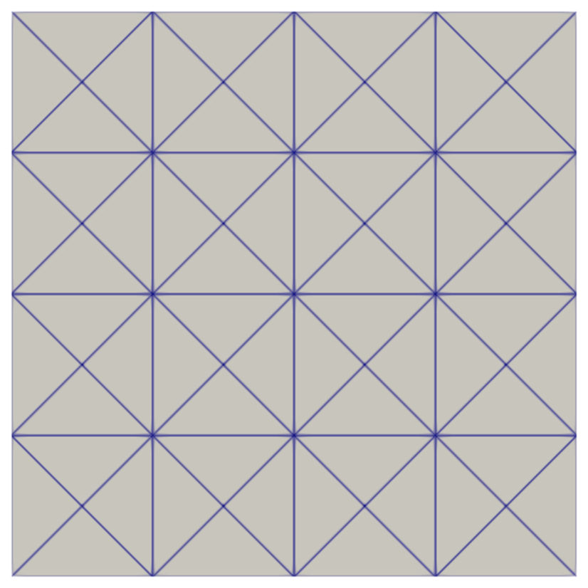
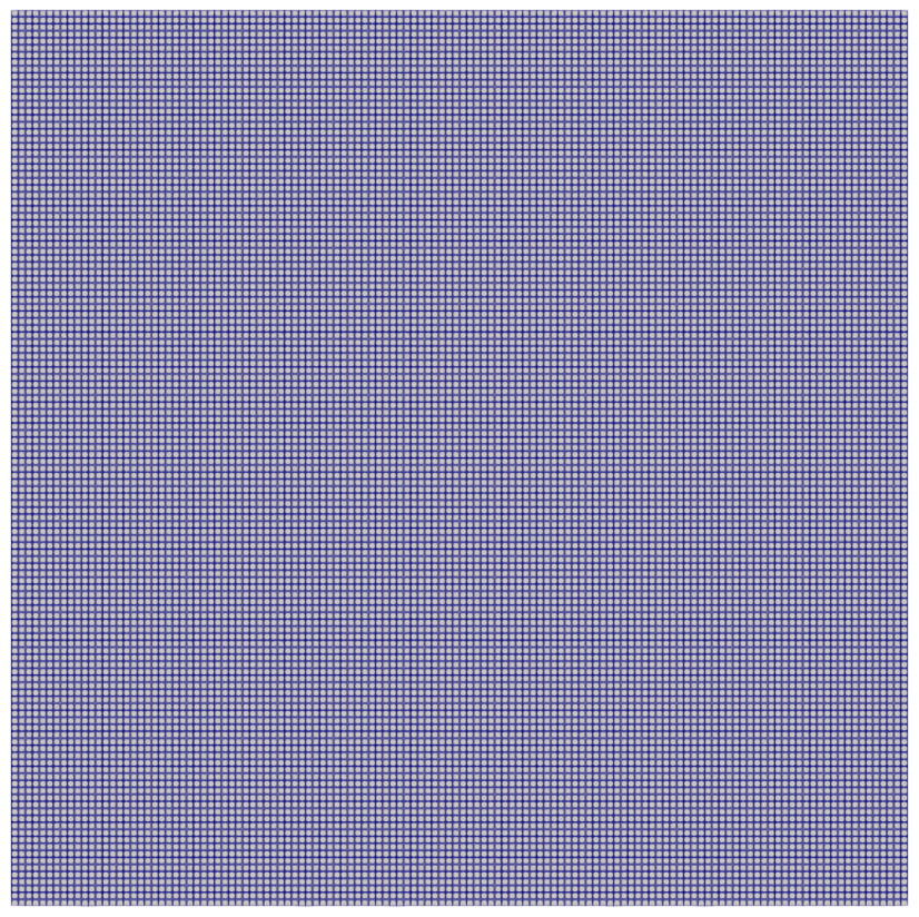
Each sub-net uses the following hyper-parameters: number of residual blocks: $2$, number of layers in each residual block: $4$, growth rate: $32$, and number of features: $32$. The inputs to the model consist of LR data $(u_{x},u_{y},P_{xx},P_{yy},P_{xy},P_{yx})$ obtained by running simulations on a coarse mesh (see Fig. 2(b)) and then interpolating the solution (using FEM basis functions) on a $32\times 32$ structured grid. The outputs of the framework correspond to the HR data on a $128\times 128$ structured grid shown in Figure 2(c).

3.2 Constructing the loss function

In the absence of any HR labeled data, the network’s total loss $\mathcal{L}$ is obtained from the physics-based constraints of the system - governing PDEs, constitutive law, and boundary/initial conditions. However, it has been well documented that presence of multiple components in $\mathcal{L}$ gives rise to competing effects amongst them leading to convergence issues during the training of the model [BK21, WTP20, AKDC22]. Therefore, in this work, we choose to impose the boundary conditions in a “hard” manner thus eliminating their contribution from total loss $\mathcal{L}$.

For each unknown field component, the boundary conditions are imposed in a hard manner by using a composite scheme which consists of using a function $\mathcal{F}$ that satisfies the boundary condition, a function $\mathcal{G}$ that is zero on the Dirichlet boundaries, and the output $\mathcal{N}$ of the DL model. The final solution to the super-resolution problem for each output field $\Phi\in\{u_{x},u_{y},P_{xx},P_{yy},P_{xy},P_{yx}\}$ is then given as follows:

$$\begin{split}\Phi(X,Y)&=\mathcal{F}_{\Phi}(X,Y)+\mathcal{N}_{\Phi}(X,Y)\cdot\mathcal{G}_{\Phi}(X,Y)\end{split}$$ (4)

For complicated geometries and boundary conditions, the above strategy can be generalized to obtain functions $\mathcal{F}$ and $\mathcal{G}$ as outputs of separate DL models as shown in [RSL21]. For finite deformation material modeling, the physical constraint $J(X,Y)>0$ has to be strictly enforced as well. Since the boundary conditions are satisfied exactly, the total loss $\mathcal{L}$ is given as follows

$$\mathcal{L}=\lambda_{1}\,\underbrace{L(Div\bm{P},\,\bm{0})}_{\textrm{PDE}}+\lambda_{2}\,\underbrace{L(\bm{P},\,\mu\left(\bm{B}-\bm{I}\right))}_{\textrm{Constitutive law}}+\underbrace{\mathcal{L}_{J}}_{J>0},$$ (5)

where $L(P,Q)$ measures the mean absolute error (MAE) for the prediction $P$ and target $Q$. The constraint loss $\mathcal{L}_{J}$ is given as $\mathcal{L}_{J}=||\min(0,det\bm{F})||_{1}$ where $||(\cdot)||_{1}$ denotes the $L^{1}$ norm of the quantity $(\cdot)$. We utilize fourth order finite difference scheme to evaluate the derivatives of the fields on the fine mesh.

The current work involving super-resolution to nonlinear solid mechanics problems has a significantly distinguishing feature from its application to resolving fluid flow in that any technique for initialization of model weights would not satisfy the physical constraint $J(X,Y)>0$ initially. This leads to nonconvergence during model training using any optimization strategies such as the family of gradient descent methods. To remedy this, we first train the model to satisfy the constraint exactly ($\mathcal{L}_{J}=0$) by setting $\lambda_{1}=\lambda_{2}=0$ during the few initial epochs of the training. After that, we choose $\lambda_{1}=1$ and $\lambda_{2}=10$ based on the heuristics that the equilibrium equation (1) also depends the derivatives of $\mu$ for heterogeneous materials.

(a)

(b)

(c)

Figure 2: a) Schematic showing the geometry and the applied boundary conditions. b) Coarse triangular mesh with $41$ nodes. c) $128\times 128$ fine mesh with $16384$ nodes. The LR data is refined by $\approx 400$ times.

The framework is implemented and trained using PyTorch framework [PGM⁺19]. The network’s total loss $\mathcal{L}$ is minimized by iteratively updating its trainable parameters. The whole training process consists of two stages: i) Initial convergence using Adam optimizer [KB15] with an initial learning rate $\eta=10^{-3}$, and ii) use of L-BFGS optimizer until the loss finally converges to a small value. While using Adam optimizer, the learning rate is also adaptively reduced by using ReduceLROnPlateau scheduler with the patience set to $40$. The source code for the proposed framework along with the dataset used in this research can be found at https://github.com/sairajat/SuperResolutionFiniteDeformation/  upon acceptance of this paper.

LR input

Bicubic

PhySRNet

HR reference

LR input

Bicubic

PhySRNet

HR reference

Figure 3: The color contours of displacement vector and stress tensor components in two-dimensional elastic deformation reconstructed with physics-informed super-resolution frameworks. Values below the plots indicate the error $e$. In both the blocks, the LR input data, HR ground truth data, bicubic interpolation, and the RDN output are plotted from the left to right.

4 Results & Discussion

4.1 Synthesis of low-resolution data

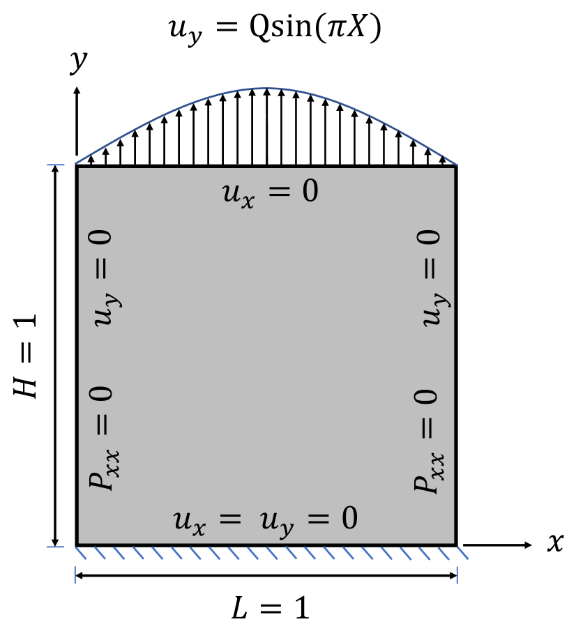
To illustrate the application of the proposed approach, an example problem is setup as follows: We consider an isotropic body deforming quasi-statically under plane strain conditions subjected to the loading boundary conditions as shown in Fig. 2(a). The body force vector $\bm{b}=(b_{x},b_{y})$ is given as

$$b_{x} =\mu_{s}\left[9\pi^{2}\cos(2\pi X)\sin(\pi Y)-\pi\cos(\pi X)QY^{3}\right],$$

$$b_{y} =\mu_{s}\left[-6\sin(\pi X)QY^{2}+2\pi^{2}\sin(2\pi X)\cos(\pi Y)+\,0.25\pi^{2}\sin(\pi X)QY^{4}\right],$$

where $\mu_{s}$ is taken to be $0.50$. The shear modulus $\mu(X,Y)$ of the material is taken to be

$$\mu=\frac{\mu_{s}}{2}\left[3+\sin(2\pi kX)\sin(2\pi kY)\right];\leavevmode\nobreak\ \leavevmode\nobreak\ k=5,$$ (6)

to represent a body with heterogeneous material properties. The scalar $Q\in[0.02,0.20]$ directly affects the magnitudes of boundary conditions (see Fig. 2(a)) and the body force $\bm{b}$. In this work, we use the following analytical forms of the functions $\mathcal{F}$ and $\mathcal{G}$ that ensure satisfaction of the boundary conditions

$$\mathcal{G}_{P_{xx}}=X\,(1-X)\leavevmode\nobreak\ \leavevmode\nobreak\ ;\leavevmode\nobreak\ \leavevmode\nobreak\ \mathcal{G}_{u_{x}}=Y\,(1-Y)\leavevmode\nobreak\ \leavevmode\nobreak\ ;\leavevmode\nobreak\ \leavevmode\nobreak\ \mathcal{G}_{u_{y}}=XY(1-X)(1-Y).$$

The ground truth data is generated by solving the system of equations (1) on a coarse mesh (shown in Fig. 2) using Finite Element Method in Fenics [ABH⁺15] for $100$ regularly sampled values of $Q$. The data is then randomly split in a $80:20$ ratio for training and test purposes.

4.2 Application to hyperelasticity

We now demonstrate the effectiveness of PhySRNet by applying it to reconstruct the HR displacement and stress fields for the problem setup discussed in section 4.1. The framework takes the coarse mesh solution fields interpolated to a $32\times 32$ grid as inputs and outputs the solution fields on a $128\times 128$ structured grid which is approximately $\!400$ times finer than the coarse mesh. We note that the framework presented herein can be generalized to work with non-rectangular domains by utilizing elliptic coordinate transformation as outlined in [GSW20].

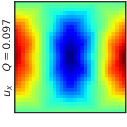
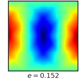
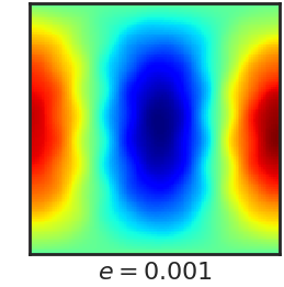
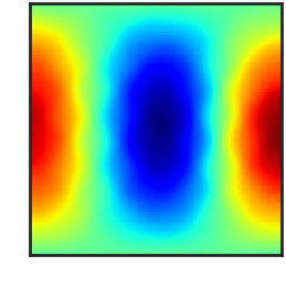
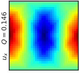
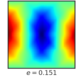
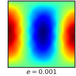
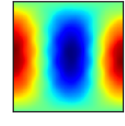
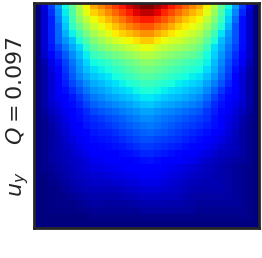
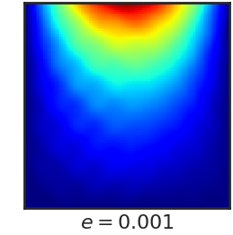
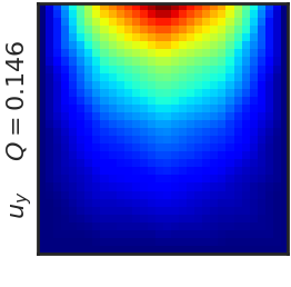
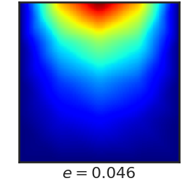
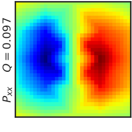
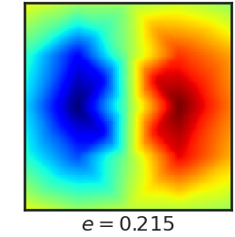
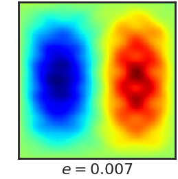
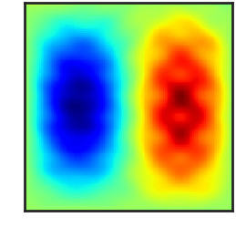
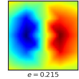
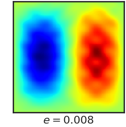
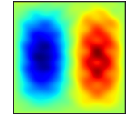
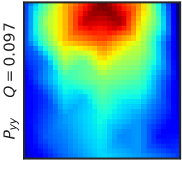
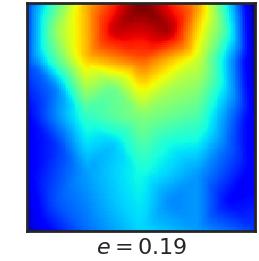
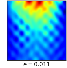
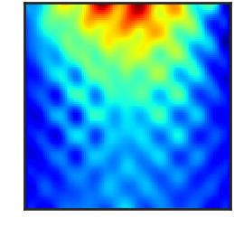
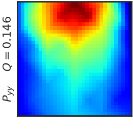
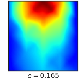
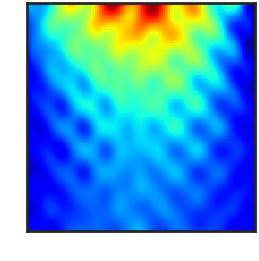
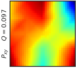
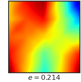
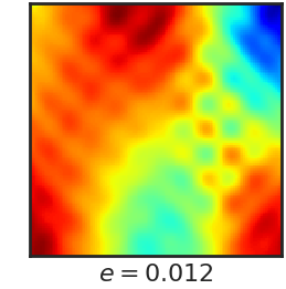
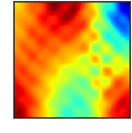
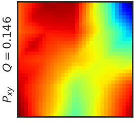
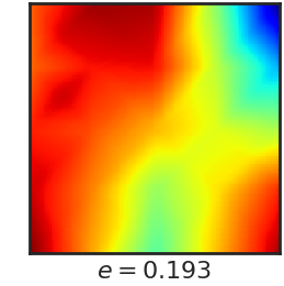
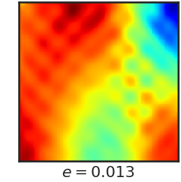
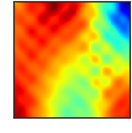
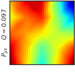
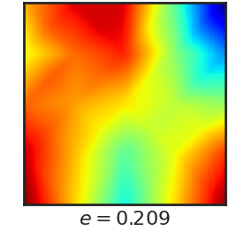
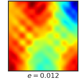
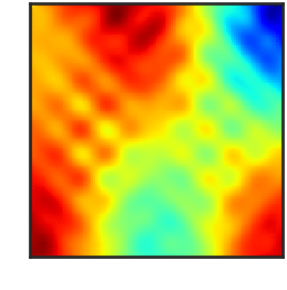
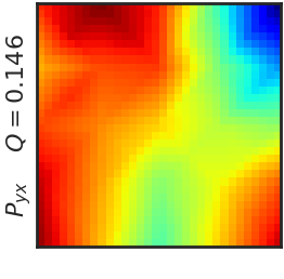
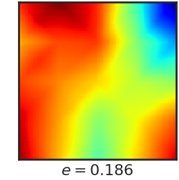
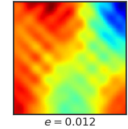
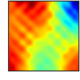
Figure 3 presents the results for the reconstructed displacement and stress fields obtained from PhySRNet for $2$ different values of $Q$. A simple bicubic interpolation of the solution fields and the HR reference data are plotted for comparison. We note that the HR reference data is used only for the comparison with the model outputs. The figure clearly show that the reconstructed solutions fields are in great agreement with the HR reference data. The model is successfully able to resolve the spatial variation in the output fields even though the LR inputs lacked such variation. To quantitatively measure the accuracy, we define an error measure $e$ as

$$e=\frac{||\mathcal{I}^{HR}-\hat{\mathcal{I}}^{HR}||_{L^{2}}}{||\mathcal{I}^{HR}||_{L^{2}}},$$ (7)

where $\hat{\mathcal{I}}^{HR}$ denotes the framework predictions. The value of $e$ is reported underneath the reconstructed fields obtained using the PhySRNet and the bicubic interpolation. As can be seen from figure 3, the error $e$ is larger for data obtained from bicubic interpolation method since the outputs may not faithfully satisfy the governing laws of the system. The small values of $e$ for the model predictions signify that the reconstructed HR outputs obtained from PhySRNet almost match the accuracy of an advanced numerical solver running at $400$ times the coarse mesh resolution. Therefore, we can conclude that PhySRNet successfully enhanced the spatial resolution of the solution fields while ensuring that they satisfy the governing laws of the system.

5 Conclusion & future work

In summary, we successfully trained and evaluated a physics-informed deep learning based super-resolution framework (PhySRNet) to reconstruct the deformation fields in a heterogeneous body undergoing hyperelastic deformation without requiring any HR labeled data. The approach is successfully able to learn high-resolution spatial variation of displacement and stress fields from their low-resolution counterparts for the example problem discussed. We show that the outputs from the PhySRNet match the accuracy of an advanced numerical solver running at $400$ times the coarse mesh resolution (see Figs. 2(b) and 2(c)). This approach exemplifies how machine-learning can be leveraged alongside numerical simulations to reduce the computational complexity and accelerate scientific discovery and engineering design without sacrificing accuracy.

While the current work focuses on nonlinear quasi-static problems, the future work aims to extend the framework for both spatial and temporal super-resolution of (unsteady) elastodynamics problems in two and three dimensions. Moreover, we also aim to modify the architecture of the PhySRNet to explore if a sequence of low-resolution data inputs could help to further improve the quality of the reconstruction.

References

- [AA20a] Rajat Arora and Amit Acharya. Dislocation pattern formation in finite deformation crystal plasticity. International Journal of Solids and Structures, 184:114–135, 2020.
- [AA20b] Rajat Arora and Amit Acharya. A unification of finite deformation J2 Von-Mises plasticity and quantitative dislocation mechanics. Journal of the Mechanics and Physics of Solids, 143:104050, 2020.
- [AAA22] Abhishek Arora, Rajat Arora, and Amit Acharya. Mechanics of micropillar confined thin film plasticity. arXiv preprint arXiv:2202.06410, 2022.
- [ABH+15] Martin Alnæs, Jan Blechta, Johan Hake, August Johansson, Benjamin Kehlet, Anders Logg, Chris Richardson, Johannes Ring, Marie E Rognes, and Garth N Wells. The fenics project version 1.5. Archive of Numerical Software, 3(100), 2015.
- [AKDC22] Rajat Arora, Pratik Kakkar, Biswadip Dey, and Amit Chakraborty. Physics-informed neural networks for modeling rate-and temperature-dependent plasticity. arXiv preprint arXiv:2201.08363, 2022.
- [Aro19] Rajat Arora. Computational Approximation of Mesoscale Field Dislocation Mechanics at Finite Deformation. PhD thesis, Carnegie Mellon University, 2019.
- [Aro21] Rajat Arora. Machine learning-accelerated computational solid mechanics: Application to linear elasticity. arXiv preprint arXiv:2112.08676, 2021.
- [AZA20] Rajat Arora, Xiaohan Zhang, and Amit Acharya. Finite element approximation of finite deformation dislocation mechanics. Computer Methods in Applied Mechanics and Engineering, 367:113076, 2020.
- [BGL+19] Mathis Bode, Michael Gauding, Zeyu Lian, Dominik Denker, Marco Davidovic, Konstantin Kleinheinz, Jenia Jitsev, and Heinz Pitsch. Using physics-informed super-resolution generative adversarial networks for subgrid modeling in turbulent reactive flows. arXiv preprint arXiv:1911.11380, 2019.
- [BK21] Rafael Bischof and Michael Kraus. Multi-objective loss balancing for physics-informed deep learning. arXiv preprint arXiv:2110.09813, 2021.
- [BLG94] Ted Belytschko, Yun Yun Lu, and Lei Gu. Element-free galerkin methods. International journal for numerical methods in engineering, 37(2):229–256, 1994.
- [CHB09] J Austin Cottrell, Thomas JR Hughes, and Yuri Bazilevs. Isogeometric analysis: toward integration of CAD and FEA. John Wiley & Sons, 2009.
- [DHLK19] Zhiwen Deng, Chuangxin He, Yingzheng Liu, and Kyung Chun Kim. Super-resolution reconstruction of turbulent velocity fields using a generative adversarial network-based artificial intelligence framework. Physics of Fluids, 31(12):125111, 2019.
- [DLHT14] Chao Dong, Chen Change Loy, Kaiming He, and Xiaoou Tang. Learning a deep convolutional network for image super-resolution. In European conference on computer vision, pages 184–199. Springer, 2014.
- [EAK+20] Soheil Esmaeilzadeh, Kamyar Azizzadenesheli, Karthik Kashinath, Mustafa Mustafa, Hamdi A Tchelepi, Philip Marcus, Mr Prabhat, Anima Anandkumar, et al. Meshfreeflownet: a physics-constrained deep continuous space-time super-resolution framework. In SC20: International Conference for High Performance Computing, Networking, Storage and Analysis, pages 1–15. IEEE, 2020.
- [FFT19] Kai Fukami, Koji Fukagata, and Kunihiko Taira. Super-resolution analysis with machine learning for low-resolution flow data. In 11th International Symposium on Turbulence and Shear Flow Phenomena, TSFP 2019, 2019.
- [FFT21] Kai Fukami, Koji Fukagata, and Kunihiko Taira. Machine-learning-based spatio-temporal super resolution reconstruction of turbulent flows. Journal of Fluid Mechanics, 909, 2021.
- [FMAH94] N. A. Fleck, G. M. Muller, M. F. Ashby, and J. W. Hutchinson. Strain gradient plasticity: Theory and experiment. Acta Metallurgica et Materialia, 42(2):475–487, 1994.
- [FTJ20] Ari Frankel, Kousuke Tachida, and Reese Jones. Prediction of the evolution of the stress field of polycrystals undergoing elastic-plastic deformation with a hybrid neural network model. Machine Learning: Science and Technology, 1(3), July 2020.
- [GFA10] Morton E. Gurtin, Eliot Fried, and Lallit Anand. The Mechanics and Thermodynamics of Continua. Cambridge University Press, 2010.
- [GSW20] Han Gao, Luning Sun, and Jian-Xun Wang. Phygeonet: Physics-informed geometry-adaptive convolutional neural networks for solving parametric pdes on irregular domain. arXiv e-prints, pages arXiv–2004, 2020.
- [GSW21] Han Gao, Luning Sun, and Jian-Xun Wang. Super-resolution and denoising of fluid flow using physics-informed convolutional neural networks without high-resolution labels. Physics of Fluids, 33(7):073603, 2021.
- [GYH+20] Li Guo, Shaojie Ye, Jun Han, Hao Zheng, Han Gao, Danny Z Chen, Jian-Xun Wang, and Chaoli Wang. Ssr-vfd: Spatial super-resolution for vector field data analysis and visualization. In Proceedings of IEEE Pacific visualization symposium, 2020.
- [HSU19] Muhammad Haris, Gregory Shakhnarovich, and Norimichi Ukita. Recurrent back-projection network for video super-resolution. In Proceedings of the IEEE/CVF Conference on Computer Vision and Pattern Recognition, pages 3897–3906, 2019.
- [Hug12] Thomas JR Hughes. The finite element method: linear static and dynamic finite element analysis. Courier Corporation, 2012.
- [JABG20] Tushar Joshi, Rajat Arora, Anup Basak, and Anurag Gupta. Equilibrium shape of misfitting precipitates with anisotropic elasticity and anisotropic interfacial energy. Modelling and Simulation in Materials Science and Engineering, 28(7):075009, 2020.
- [JCLK21] Xiaowei Jin, Shengze Cai, Hui Li, and George Em Karniadakis. Nsfnets (navier-stokes flow nets): Physics-informed neural networks for the incompressible navier-stokes equations. Journal of Computational Physics, 426:109951, 2021.
- [KB15] Diederik P. Kingma and Jimmy Ba. Adam: A Method for Stochastic Optimization. ICLR, 2015.
- [KYH+20] Georgios Kissas, Yibo Yang, Eileen Hwuang, Walter R Witschey, John A Detre, and Paris Perdikaris. Machine learning in cardiovascular flows modeling: Predicting arterial blood pressure from non-invasive 4d flow mri data using physics-informed neural networks. Computer Methods in Applied Mechanics and Engineering, 358:112623, 2020.
- [LHAY17] Wei-Sheng Lai, Jia-Bin Huang, Narendra Ahuja, and Ming-Hsuan Yang. Deep laplacian pyramid networks for fast and accurate super-resolution. In Proceedings of the IEEE conference on computer vision and pattern recognition, pages 624–632, 2017.
- [LJZ95] Wing Kam Liu, Sukky Jun, and Yi Fei Zhang. Reproducing kernel particle methods. International journal for numerical methods in fluids, 20(8-9):1081–1106, 1995.
- [PGM+19] Adam Paszke, Sam Gross, Francisco Massa, Adam Lerer, James Bradbury, Gregory Chanan, Trevor Killeen, Zeming Lin, Natalia Gimelshein, Luca Antiga, Alban Desmaison, Andreas Kopf, Edward Yang, Zachary DeVito, Martin Raison, Alykhan Tejani, Sasank Chilamkurthy, Benoit Steiner, Lu Fang, Junjie Bai, and Soumith Chintala. Pytorch: An imperative style, high-performance deep learning library. In H. Wallach, H. Larochelle, A. Beygelzimer, F. d'Alché-Buc, E. Fox, and R. Garnett, editors, Advances in Neural Information Processing Systems 32, pages 8024–8035. Curran Associates, Inc., 2019.
- [RPK17] Maziar Raissi, Paris Perdikaris, and George Em Karniadakis. Physics informed deep learning (part i): Data-driven solutions of nonlinear partial differential equations. arXiv preprint arXiv:1711.10561, 2017.
- [RPK19] Maziar Raissi, Paris Perdikaris, and George E Karniadakis. Physics-informed neural networks: A deep learning framework for solving forward and inverse problems involving nonlinear partial differential equations. Journal of Computational Physics, 378:686–707, 2019.
- [RSL20] Chengping Rao, Hao Sun, and Yang Liu. Physics-informed deep learning for incompressible laminar flows. Theoretical and Applied Mechanics Letters, 10(3):207–212, 2020.
- [RSL21] Chengping Rao, Hao Sun, and Yang Liu. Physics-informed deep learning for computational elastodynamics without labeled data. Journal of Engineering Mechanics, 147(8):04021043, 2021.
- [SCYP+20] Francisco Sahli Costabal, Yibo Yang, Paris Perdikaris, Daniel E Hurtado, and Ellen Kuhl. Physics-informed neural networks for cardiac activation mapping. Frontiers in Physics, 8:42, 2020.
- [SGPW20] Luning Sun, Han Gao, Shaowu Pan, and Jian-Xun Wang. Surrogate modeling for fluid flows based on physics-constrained deep learning without simulation data. Computer Methods in Applied Mechanics and Engineering, 361:112732, 2020.
- [SLDN22] Ankit Shrivastava, Jingxiao Liu, Kaushik Dayal, and Hae Young Noh. Predicting peak stresses in microstructured materials using convolutional encoder–decoder learning. Mathematics and Mechanics of Solids, page 10812865211055504, 2022.
- [SW20] Luning Sun and Jian-Xun Wang. Physics-constrained bayesian neural network for fluid flow reconstruction with sparse and noisy data. Theoretical and Applied Mechanics Letters, 10(3):161–169, 2020.
- [SWB+20] Akshay Subramaniam, Man Long Wong, Raunak D Borker, Sravya Nimmagadda, and Sanjiva K Lele. Turbulence enrichment using physics-informed generative adversarial networks. arXiv preprint arXiv:2003.01907, 2020.
- [WTP20] Sifan Wang, Yujun Teng, and Paris Perdikaris. Understanding and mitigating gradient pathologies in physics-informed neural networks. arXiv preprint arXiv:2001.04536, 2020.
- [XFCT18] You Xie, Erik Franz, Mengyu Chu, and Nils Thuerey. tempogan: A temporally coherent, volumetric gan for super-resolution fluid flow. ACM Transactions on Graphics (TOG), 37(4):1–15, 2018.
- [ZLY21] Qiming Zhu, Zeliang Liu, and Jinhui Yan. Machine learning for metal additive manufacturing: predicting temperature and melt pool fluid dynamics using physics-informed neural networks. Computational Mechanics, 67(2):619–635, 2021.
- [ZTK+18] Yulun Zhang, Yapeng Tian, Yu Kong, Bineng Zhong, and Yun Fu. Residual dense network for image super-resolution. In Proceedings of the IEEE conference on computer vision and pattern recognition, pages 2472–2481, 2018.