MEAD: A Multi-Armed Approach for Evaluation of Adversarial Examples Detectors

Abstract

Detection of adversarial examples has been a hot topic in the last years due to its importance for safely deploying machine learning algorithms in critical applications. However, the detection methods are generally validated by assuming a single implicitly known attack strategy, which does not necessarily account for real-life threats. Indeed, this can lead to an overoptimistic assessment of the detectors’ performance and may induce some bias in the comparison between competing detection schemes. We propose a novel multi-armed framework, called MEAD, for evaluating detectors based on several attack strategies to overcome this limitation. Among them, we make use of three new objectives to generate attacks. The proposed performance metric is based on the worst-case scenario: detection is successful if and only if all different attacks are correctly recognized. Empirically, we show the effectiveness of our approach. Moreover, the poor performance obtained for state-of-the-art detectors opens a new exciting line of research.

1 Introduction

Despite recent advances in the application of machine learning, the vulnerability of deep learning models to maliciously crafted examples  [34] is still an open problem of great interest for safety-critical applications [2, 4, 10, 39]. Over time, a large body of literature has been produced on the topic of defense methods against adversarial examples. On the one hand, interest in detecting adversarial examples given a pre-trained model is gaining momentum [17, 24, 27]. On the other hand, several techniques have been proposed to train models with improved robustness to future attacks [26, 31, 38]. Interestingly, Croce et al. have recently pointed out that, due to the large number of proposed methods, the problem of crafting an objective approach to evaluate the quality of methods to train robust models is not trivial. To this end, they have presented RobustBench [9], a standardized benchmark to assess adversarial robustness. To the best of our knowledge, we claim that an equivalent benchmark does not exist in the case of methods to detect adversarial examples given a pre-trained model. Therefore, in this work, we provide a general framework to evaluate the performance of adversarial detection methods. Our idea stems from the following key observation. Generally, the performance of current state-of-the-art (SOTA) adversarial examples detection methods is evaluated assuming a unique and thus implicitly known attack strategy, which does not necessarily correspond to real-life threats. We further argue that this type of evaluation has two main flaws: the performance of detection methods may be overestimated, and the comparison between detection schemes may be biased. We propose a two-fold solution to overcome the aforementioned limitations, leading to a less biased evaluation of different approaches. This is accomplished by evaluating the detection methods on simultaneous attacks on the target classification model using different adversarial strategies, considering the most popular attack techniques in the literature, and incorporating three new attack objectives to extend the generality of the proposed framework. Indeed, we argue that additional attack objectives result in new types of adversarial examples that cannot be constructed otherwise. In particular, we translate such an evaluation scheme in MEAD.

MEAD is a novel evaluation framework that uses a simple but still effective “multi-armed” attack to remove the implicit assumption that detectors know the attacker’s strategy. More specifically, for each natural sample, we consider the detection to be successful if and only if the detector is able to identify all the different attacks perpetrated by perturbing the testing sample at hand. We deploy the proposed framework to evaluate the performance of SOTA adversarial examples detection methods over multiple benchmarks of visual datasets. Overall, the collected results are consistent throughout the experiments. The main takeaway is that considering a multi-armed evaluation criterion exposes the weakness of SOTA detection methods, yielding, in some cases, relatively poor performances. The proposed framework, although not exhaustive, sheds light on the fact that evaluations so far presented in the literature are highly biased and unrealistic. Indeed, the same detector achieves very different performances when it is informed about the current attack as opposed to when it is not. Not surprisingly, supervised and unsupervised methods achieve comparable performances with the multi-armed framework, meaning that training the detectors knowing a specific attack used at testing time does not generalize to other attacks enough. Indeed the goal of MEAD is not to show that new attacks can always fool robust classifiers but to show that the detectors that may work well when evaluated with a unique attack strategy end up being defeated by new attacks.

1.1 Summary of contributions

We propose MEAD, a novel multi-armed evaluation framework for adversarial examples detectors involving several attackers to ensure that the detector is not overfitted to a particular attack strategy. The proposed metric is based on the following criterion. Each adversarial sample is correctly detected if and only if all the possible attacks on it are successfully detected. We show that this approach is less biased and yields a more effective metric than the one obtained by assuming only a single attack at evaluation time (see Sec. 4).

We make use of three new objective functions which, to the best of our knowledge, have never been used for the purpose of generating adversarial examples at testing time. These are KL divergence, Gini Impurity and Fisher-Rao distance. Moreover, we argue that each of them contributes to jointly creating competitive attacks that cannot be created by a single function (see Sec. 3.2).

We perform an extensive numerical evaluation of SOTA and uncover their limitations, suggesting new research perspectives in this research line (see Sec. 5).

The remaining paper is organized as follows. First, in Sec. 2, we present a detailed overview of the recent related works. In Sec. 3, we describe the adversarial problem along with the new objectives we introduce within the proposed evaluation framework, MEAD, which is further explained in Sec. 4. We extensively experimentally validate MEAD in Sec. 5. Finally, in Sec. 6, we provide the summary together with concluding remarks.

2 Related Works

State-of-the-art methods to detect adversarial examples can be separated in two main groups [2]: supervised and unsupervised methods. In the supervised setting, detectors can make use of the knowledge of the attacker’s procedure. The network invariant model approach extracts natural and adversarial features from the activation values of the network’s layers [7, 23, 28], while the statistical approach extract features using statistical tools (e.g. maximum mean discrepancy [16], PCA [21], kernel density estimation [13], local intrinsic dimensionality [25], model uncertainty [13] or natural scene statistics [17]) to separate in-training and out-of-training data distribution/manifolds. To overcome the intrinsic limitation of the necessity to have prior knowledge of attacks, unsupervised detection methods consider only clean data at training time. The features extraction can rely on different techniques (e.g., feature squeezing [22, 36], denoiser approach [27], network invariant [24], auxiliary model [1, 32, 40]). Moreover, detection methods of adversarial examples can also act on the underlying classifier by considering a novel training procedure (e.g., reverse cross-entropy [30]; the rejection option [1, 32]) and a thresholding test strategy towards robust detection of adversarial examples. Finally, detection methods can also be impacted by the learning task of the underlying network (e.g., for human recognition tasks [35]).

2.1 Considered detection methods

Supervised methods. Supervised methods can make use of the knowledge of how adversarial examples are crafted. They often use statistical properties of either the input samples or the output of hidden layers. NSS [17] extract the Natural Scene Statistics of the natural and adversarial examples, while LID [25] extract the local intrinsic dimensionality features of the output of hidden layers for natural, noisy and adversarial inputs. KD-BU [13] estimates the kernel density of the last hidden layer in the feature space, then estimates the bayesian uncertainty of the input sample, following the intuition that the adversarial examples lie off the data manifold. Once those features are extracted, all methods train a detector to discriminate between natural and adversarial samples.

Unsupervised methods. Unsupervised method can only rely on features of the natural samples. FS [36] is an unsupervised method that uses feature squeezing to compare the model’s predictions. Following the idea of estimating the distance between the test examples and the boundary of the manifold of normal examples, MagNet [27] comprises detectors based on reconstruction error and detectors based on probability divergence.

2.2 Considered attack mechanisms

The attack mechanisms can be divided into two categories: whitebox attacks, where the adversary has complete knowledge about the targeted classifier (its architecture and weights), and blackbox attacks where the adversary has no access to the internals of the target classifier.

Whitebox attacks. One of the first introduced attack mechanisms is what we call the Fast Gradient Sign Method (FGSM) [14]. It relies on computing the direction gradient of a given objective function with respect to (w.r.t.) the input of the targeted classifier and modifying the original sample following it. This method has been improved multiple times. Basic Iterative Method (BIM) [19] and Projected Gradient Descent (PGD) [26] are two iteration extensions of FGSM. They were introduced at the same time, and the main difference between the two is that BIM initializes the algorithm to the original sample while PGD initializes it to the original sample plus a random noise. Despite that PGD was introduced under the L_∞-norm constraint, it can be extended to any L_p-norm constraint. Deepfool (DF) [29] was later introduced. It is an iterative method based on a local linearization of the targeted classifier and the resolution of this simplified problem. Finally, the Carlini&Wagner method (CW) aims at finding the smaller noise to solve the adversarial problem. To do so, they present a relaxation based on the minimization of specific objectives that can be chosen depending on the attacker’s goal.

Blackbox attacks. Blackbox attacks can only rely on queries to attack specific models. Square Attack (SA) [3] is an iterative method that randomly searches for a perturbation that will increase the attacker’s objective at each step, Hop Skip Jump (HOP) [8] tries to estimate the gradient direction to perturb, and Spatial Transformation Attack (STA) [12] applies small translations and rotations to the original sample to fool the targeted classifier.

3 Adversarial Examples and Novel Objectives

Let $\mathcal{X}\subseteq\mathbb{R}^{d}$ be the input space and let $\mathcal{Y}=\{1,\dots,C\}$ be the label space related to some task of interest. We denote by $P_{XY}$ the unknown data distribution over $\mathcal{X}\times\mathcal{Y}$. Throughout the paper we refer to the classifier $q_{\widehat{Y}|X}(y|\mathbf{x};\theta)$ to be the parametric soft-probability model, where $\theta\in\Theta$ are the parameters, $y\in\mathcal{Y}$ the label and $f_{\theta}:\mathcal{X}\rightarrow\mathcal{Y}$ s.t. $f_{\theta}(\mathbf{x})=\arg\max_{y\in\mathcal{Y}}q_{\widehat{Y}|X}(y|\mathbf{x};\theta)$ to be its induced hard decision. Finally, we denote by $\mathbf{x}^{\prime}\in\mathbb{R}^{d}$ an adversarial example, by $\ell(\mathbf{x},\mathbf{x}^{\prime};\theta)$ the objective function used by the attacker to generate that sample, and $a_{\ell}(\cdot;\varepsilon,p)$ the attack mechanism according to a objective function $\ell$, with $\varepsilon$ the maximal perturbation allow and $p$ the L_p-norm constraint.

3.1 Generating adversarial examples

Adversarial examples are slightly modified inputs that can fool a target classifier. Concretely, Szegedy et al. [33] define the adversarial generation problem as:

$$\mathbf{x}^{\prime}=\underset{\mathbf{x}^{\prime}\in\mathbb{R}^{d}\,:\,\lVert\mathbf{x}^{\prime}-\mathbf{x}\rVert_{p}<\varepsilon}{\operatorname*{arg\,min}}\lVert\mathbf{x}^{\prime}-\mathbf{x}\rVert\text{~{}~{}s.t.~{}~{}}f_{\theta}(\mathbf{x}^{\prime})\neq y,$$ (1)

where $y$ is the true label (supervision) associated to the sample $\mathbf{x}$. Since this problem is difficult to tackle, it is commonly relaxed as follows [6]:

$$a_{\ell}(\mathbf{x};\varepsilon,p)\equiv~{}\mathbf{x}^{\prime}_{\ell}=\underset{\mathbf{x}^{\prime}_{\ell}\in\mathbb{R}^{d}\,:\,\lVert\mathbf{x}^{\prime}_{\ell}-\mathbf{x}\rVert_{p}<\varepsilon}{\operatorname*{arg\,max}}\ell(\mathbf{x},\mathbf{x}^{\prime}_{\ell};\mathbf{\theta).}$$ (2)

It is worth to emphasize that the choice of the objective $\ell(\mathbf{x},\mathbf{x}^{\prime}_{\ell};\theta)$ plays a crucial role in generating powerful adversarial examples $\mathbf{x}^{\prime}_{\ell}$. The objective function $\ell$ traditionally used is the Adversarial Cross-Entropy (ACE) [26]:

$$\ell_{\text{ACE}}(\mathbf{x},\mathbf{x}^{\prime}_{\ell};\theta)=\mathbb{E}_{Y|\mathbf{x}}\big{[}-\log q_{\widehat{Y}|X}(Y|\mathbf{x}^{\prime}_{\ell};\theta)\big{]},$$ (3)

It is possible to use any objective function $\ell$ to craft adversarial samples. We present the three losses that we use to generate adversarial examples in the following. While these losses have already been considered in detection/robustness cases, to the best of our knowledge, they have never been used to craft attacks to test the performances of detection methods.

3.2 Three New Objective Functions

3.2.1 The Kullback-Leibler divergence.

The Kullback-Leibler (KL) divergence between the natural and the adversarial probability distributions has been widely used in different learning problems, as building training losses for robust models [37]. KL is defined as follows:

$$\ell_{\text{KL}}\left(\mathbf{x},\mathbf{x}^{\prime}_{\ell};\theta\right)=\mathbb{E}_{\widehat{Y}|\mathbf{x};\theta}\left[\log\left(\frac{q_{\widehat{Y}|X}(\widehat{Y}|\mathbf{x};\theta)}{q_{\widehat{Y}|X}(\widehat{Y}|\mathbf{x}^{\prime}_{\ell};\theta)}\right)\right].$$ (4)

3.2.2 The Fisher-Rao objective.

The Fisher-Rao (FR) distance is an information-geometric measure of dissimilarity between soft-predictions  [5]. It has been recently used to craft a new regularizer for robust classifiers [31]. FR can be computed as follows:

$$\ell_{\text{FR}}(\mathbf{x},\mathbf{x}^{\prime}_{\ell};\theta)= 2\arccos\left(\sum_{y\in\mathcal{Y}}\sqrt{q_{\widehat{Y}|X}(y|\mathbf{x};\theta)q_{\widehat{Y}|X}(y|\mathbf{x}^{\prime}_{\ell};\theta)}\right).$$ (5)

3.2.3 The Gini Impurity score.

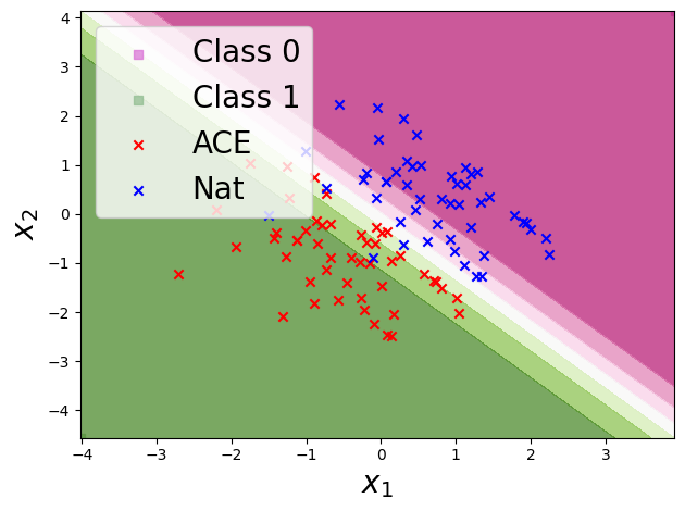
(a) Pre-trained classifier

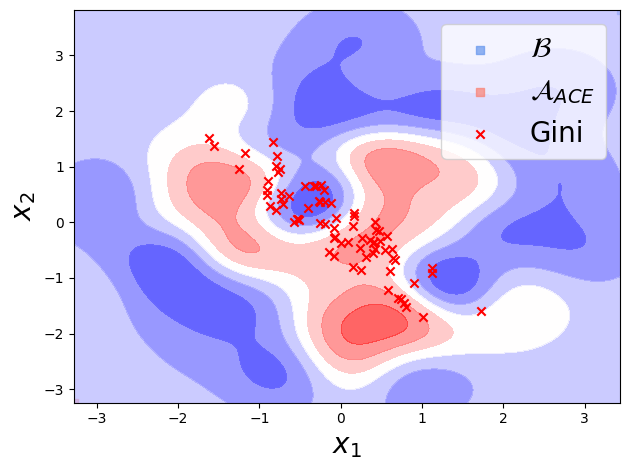
(b) Detector trained on ACE

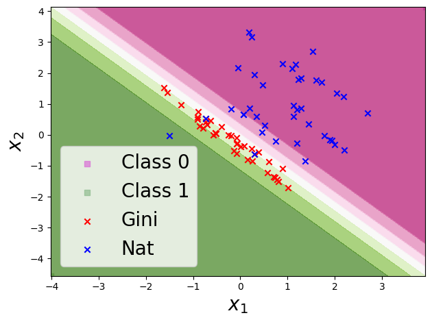
(c) Pre-trained classifier

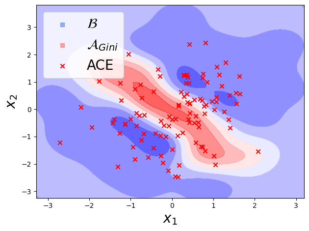
(d) Detector trained on Gini

Figure 1: Decision boundary for the binary classifier 1(a)-1(c): the decision region for class 1 is green, the decision region of class 0 is pink. The natural testing samples belonging to class 0 are reported in blue, the corresponding adversarial examples crafted using ACE (1(a)) and Gini Impurity (1(c)) in red. Decision boundary of the detectors 1(b)-1(d): $\mathcal{B}$, the decision region of the natural examples; $\mathcal{A}_{\ell}$, reported in red shades, the decision region of the adversarial examples when the detector is trained on data points crafted via $\ell\in\{\text{ACE},\text{~{}Gini}\}$ as objective. The darker shades stand for higher confidence. The red points represent the adversarial examples created with the opposite loss (respectively $\ell\in\{\text{Gini},\text{~{}ACE}\}$).

The Gini Impurity score approximates the probability of incorrectly classifying the input $\mathbf{x}$ if it was randomly labeled according to the model’s output distribution $q_{\widehat{Y}|X}(y|\mathbf{x}^{\prime}_{\ell};\theta)$. It was recently used in [15] to determine whether a sample is correctly or incorrectly classified.

$$\ell_{\text{Gini}}(\cdot,\mathbf{x}^{\prime}_{\ell};\theta) =1-\sqrt{\underset{y\in\mathcal{Y}}{\sum}q^{2}_{\widehat{Y}|X}(y|\mathbf{x}^{\prime}_{\ell};\theta)}.$$ (6)

3.3 A case study: ACE vs. Gini Impurity

In Figure 1 we provide insights on why we need to evaluate the detectors on attacks crafted through different objectives. We create a synthetic dataset that consists of 300 data points drawn from $\mathcal{N}_{0}=\mathcal{N}(\mu_{0},\sigma^{2}\mathbf{I})$ and 300 data points drawn from $\mathcal{N}_{1}=\mathcal{N}(\mu_{1},\sigma^{2}\mathbf{I})$, where $\mu_{0}=[1~{}1]$, $\mu_{1}=[-1~{}-1]$ and $\sigma=1$. To each data point $\mathbf{x}$ is assigned true label $0$ or $1$ depending on whether $\mathbf{x}\sim\mathcal{N}_{0}$ or $\mathbf{x}\sim\mathcal{N}_{1}$, respectively. The data points have been split between the training set ($70\%$) and the testing set ($30\%$). We finally train a simple binary classifier with one single hidden layer and a learning rate of 0.01 for 20 epochs. We attack the classifier by generating adversarial examples with PGD under the L_∞-norm constraints with $\varepsilon=1.2$ for the ACE attacks and $\varepsilon=5$ for the Gini Impurity attacks to have a classification accuracy (classifier performance) of $50\%$ on the corrupted data points. In Figure 1(a)-1(c) we plot the decision boundary of the binary classifier together with the adversarial and natural examples belonging to class 0. As can be seen, ACE creates points that lie in the opposite decision region with respect to the original points (Fig. 1(a)). Conversely, Gini Impurity tends to create new data points in the region of maximal uncertainty of the classifier (Fig. 1(c)). Consider the scenario where we train a simple Radial Basis Function (RBF) kernel SVM on a subset of the testing set of the natural points together with the attacked examples, generated with the ACE or the Gini Impurity score depending on the case (Fig. 1(b)-1(d)). We then test the detector on the data points originated with the opposite loss, Figure 1(b) and Figure 1(d) respectively. The decision region of the detector for natural examples is in blue, and the one for the adversarial examples is in red. The intensity of the color corresponds to the level of certainty of the detector. The accuracy of the detector on natural and adversarial data points decreases from $71\%$ to $62\%$ when changing to the opposite loss in Fig. 1(b), and from $87\%$ to $63\%$ in  Fig. 1(d). Hence, testing on samples crafted using a different loss in Eq. 2 means changing the attack and, consequently, evaluating detectors without taking into consideration this possibility leads to a more biased and unrealistic estimation of their performance. When the detector is trained on the adversarial examples created with both the losses, the accuracy is $79.8\%$ when testing on Gini and $66.3\%$ when testing on ACE, which is a better trade-off in adversarial detection performances.

The aforementioned losses will be included in the following section to design MEAD, our multi-armed evaluation framework, a new method to evaluate the performance of adversarial detection with low bias.

4 Evaluation with a Multi-Armed Attacker

Figure 2: MEAD: $\mathbf{x}$ is the natural example, $\varepsilon=5$ is the perturbation magnitude, L₁ is the norm. From the set of all the possible existing attacks $\mathcal{A}$ we consider the ones using PGD. The sifter discards all the perturbed samples that do not fool the classifier $f_{\theta}$. $d$ is the detector.

The proposed evaluation framework, MEAD, consists in testing an adversarial examples detection method on a large collection of attacks grouped w.r.t. the L_p-norm and the maximal perturbation $\varepsilon$ they consider. Each given natural input example is perturbed according to the collection of attacks. Note that, for every attack, a perturbed example is considered adversarial if and only if it fools the classifier. Otherwise, it is discarded and will not influence the evaluation. We then feed all the natural and successful adversarial examples to the detector and gather all the predictions. Finally, based on the detection decisions, we evaluate the detector according to a worst-case scenario:
i) Adversarial decision: for each natural example, we gather all the successful adversarial examples. If the detector detects all of them, then the perturbed sample is considered correctly detected (i.e., it is a true positive). However, if the detector misses at least one of them, the noisy sample is considered undetected (i.e., it is a false negative).
ii) Natural decision: for each natural sample, if the detector does not detect it, then the sample is considered correctly non-detected (i.e., it is a true negative); otherwise it is incorrectly detected (i.e., it is a false positive).

Specifically, let $\mathcal{D}_{m}=\{(\mathbf{x}_{i},y_{i})\}_{i=1}^{m}\sim P_{XY}$ be the testing set of size $m$, where $\mathbf{x}_{i}\in\mathcal{X}$ is the natural input sample and $y_{i}\in\mathcal{Y}$ is its true label. Let $d$: $\mathcal{X}\times\mathbb{R}\rightarrow\{0,1\}$ be the detection mechanism and $a_{\ell}:\mathcal{X}\times\mathbb{R}\times\{1,2,\infty\}\rightarrow\mathcal{X}$ the attack strategy according to the objective function $\ell\in\mathcal{L}$ within a selected collection of objectives $\mathcal{L}$ as described in Sec. 3. For every considered L_p-norm, $p\in\{1,2,\infty\}$, maximal perturbation $\varepsilon\in\mathbb{R}$, and every threshold $\gamma\in\mathbb{R}$:

$$TP_{\varepsilon,p}(\gamma)=\Big{\{}(\mathbf{x},y)\in\mathcal{D}_{m}:\forall\ell\in\mathcal{L}\;\{f_{\theta}\big{(}a_{\ell}(\mathbf{x})\big{)}\neq y\}~{}\wedge~{}\{d\big{(}a_{\ell}(\mathbf{x}),\gamma\big{)}=1\}\Big{\}}$$ (7)

$$FN_{\varepsilon,p}(\gamma)=\Big{\{}(\mathbf{x},y)\in\mathcal{D}_{m}:\exists\ell\in\mathcal{L}\;\{f_{\theta}\big{(}a_{\ell}(\mathbf{x})\big{)}\neq y\}~{}\wedge~{}\{d\big{(}a_{\ell}(\mathbf{x}),\gamma\big{)}=0\}\Big{\}}$$ (8)

$$TN_{\varepsilon,p}(\gamma)=\{(\mathbf{x},y)\in\mathcal{D}_{m}:d(\mathbf{x},\gamma)=0\}$$ (9)

$$FP_{\varepsilon,p}(\gamma)=\{(\mathbf{x},y)\in\mathcal{D}_{m}:d(\mathbf{x},\gamma)=1\}.$$ (10)

In Fig. 2 we provide a graphical interpretation of MEAD when the perturbation magnitude and the norm are fixed.

5 Experiments

In this section, we assess the effectiveness of the proposed evaluation framework, MEAD. The code is available at https://github.com/meadsubmission/MEAD.

CIFAR10	MEAD		ACE		KL		Gini		FR
NSS	AUROC$\uparrow$%	FPR$\downarrow_{95\%}$%	AUROC$\uparrow$%	FPR$\downarrow_{95\%}$%	AUROC$\uparrow$%	FPR$\downarrow_{95\%}$%	AUROC$\uparrow$%	FPR$\downarrow_{95\%}$%	AUROC$\uparrow$%	FPR$\downarrow_{95\%}$%
L1 Average	62.9	81.6	67.4	75.7	67.1	76.0	67.8	78.2	67.6	75.6
L2 Average	64.0	82.0	68.7	71.0	68.5	70.9	65.1	82.0	68.6	71.1
L∞ Average	71.9	62.0	76.9	40.1	77.2	39.5	73.7	59.6	74.1	57.2
No norm	88.5	38.8	88.5	38.8	88.5	38.8	88.5	38.8	88.5	38.8
KD-BU	AUROC$\uparrow$%	FPR$\downarrow_{95\%}$%	AUROC$\uparrow$%	FPR$\downarrow_{95\%}$%	AUROC$\uparrow$%	FPR$\downarrow_{95\%}$%	AUROC$\uparrow$%	FPR$\downarrow_{95\%}$%	AUROC$\uparrow$%	FPR$\downarrow_{95\%}$%
L1 Average	50.9	95.7	70.0	88.6	70.0	88.4	74.3	92.3	69.8	88.4
L2 Average	59.0	94.1	71.6	71.9	71.7	71.6	70.6	92.8	71.7	71.8
L∞ Average	36.8	96.9	64.8	92.1	68.1	91.3	53.7	95.6	67.8	91.7
No norm	65.4	94.2	65.4	94.2	65.4	94.2	65.4	94.2	65.4	94.2
LID	AUROC$\uparrow$%	FPR$\downarrow_{95\%}$%	AUROC$\uparrow$%	FPR$\downarrow_{95\%}$%	AUROC$\uparrow$%	FPR$\downarrow_{95\%}$%	AUROC$\uparrow$%	FPR$\downarrow_{95\%}$%	AUROC$\uparrow$%	FPR$\downarrow_{95\%}$%
L1 Average	50.8	95.4	69.6	82.1	69.4	82.9	88.9	49.9	69.1	83.7
L2 Average	63.5	83.1	73.7	70.1	73.4	70.7	82.5	61.3	73.2	71.3
L∞ Average	53.8	90.8	75.7	56.8	79.9	57.6	71.3	79.7	82.0	51.4
No norm	88.0	58.1	88.0	58.1	88.0	58.1	88.0	58.1	88.0	58.1
FS	AUROC$\uparrow$%	FPR$\downarrow_{95\%}$%	AUROC$\uparrow$%	FPR$\downarrow_{95\%}$%	AUROC$\uparrow$%	FPR$\downarrow_{95\%}$%	AUROC$\uparrow$%	FPR$\downarrow_{95\%}$%	AUROC$\uparrow$%	FPR$\downarrow_{95\%}$%
L1 Average	75.4	64.8	92.8	25.1	92.9	24.9	73.5	67.6	92.9	24.6
L2 Average	74.9	65.8	87.4	31.2	87.6	36.9	73.7	67.2	87.4	37.5
L∞ Average	52.7	81.1	73.0	60.1	77.5	55.7	58.2	78.8	75.7	58.5
No norm	62.7	82.5	62.7	82.5	62.7	82.5	62.7	82.5	62.7	82.5
MagNet	AUROC$\uparrow$%	FPR$\downarrow_{95\%}$%	AUROC$\uparrow$%	FPR$\downarrow_{95\%}$%	AUROC$\uparrow$%	FPR$\downarrow_{95\%}$%	AUROC$\uparrow$%	FPR$\downarrow_{95\%}$%	AUROC$\uparrow$%	FPR$\downarrow_{95\%}$%
L1 Average	49.6	93.7	49.8	93.5	49.7	93.3	50.1	93.2	49.1	93.8
L2 Average	50.9	93.1	52.3	89.6	52.3	89.4	50.5	93.3	51.8	91.4
L∞ Average	78.0	46.1	79.2	44.6	80.2	44.1	79.2	44.6	80.0	44.6
No norm	79.9	45.7	79.9	45.7	79.9	45.7	79.9	45.7	79.9	45.7

Table 1: Overall performances on CIFAR10 of all the detectors per objective and in MEAD. The worst results among all the settings is in bold; the ones in the single-armed setting is underlined. No norm denotes the group of attacks that do not depend on the norm constraint.

MNIST	MEAD		ACE		KL		Gini		FR
NSS	AUROC$\uparrow$%	FPR$\downarrow_{95\%}$%	AUROC$\uparrow$%	FPR$\downarrow_{95\%}$%	AUROC$\uparrow$%	FPR$\downarrow_{95\%}$%	AUROC$\uparrow$%	FPR$\downarrow_{95\%}$%	AUROC$\uparrow$%	FPR$\downarrow_{95\%}$%
L1 Average	96.8	9.4	97.0	8.2	97.1	8.6	97.4	7.0	97.1	8.1
L2 Average	90.3	26.5	90.7	25.8	90.8	25.4	91.4	23.7	90.6	26.5
L∞ Average	88.7	23.5	89.5	23.5	89.5	23.6	90.0	23.6	89.8	23.5
No norm	87.1	57.8	87.1	57.8	87.1	57.8	87.1	57.8	87.1	57.8
KD-BU	AUROC$\uparrow$%	FPR$\downarrow_{95\%}$%	AUROC$\uparrow$%	FPR$\downarrow_{95\%}$%	AUROC$\uparrow$%	FPR$\downarrow_{95\%}$%	AUROC$\uparrow$%	FPR$\downarrow_{95\%}$%	AUROC$\uparrow$%	FPR$\downarrow_{95\%}$%
L1 Average	45.6	95.7	59.9	93.0	59.3	93.1	61.4	92.7	58.9	93.3
L2 Average	50.3	94.8	59.9	93.0	59.7	93.1	59.3	93.2	59.8	93.0
L∞ Average	34.1	96.7	42.8	96.0	44.7	95.8	48.6	95.3	44.9	95.8
No norm	76.0	88.2	76.0	88.2	76.0	88.2	76.0	88.2	76.0	88.2
LID	AUROC$\uparrow$%	FPR$\downarrow_{95\%}$%	AUROC$\uparrow$%	FPR$\downarrow_{95\%}$%	AUROC$\uparrow$%	FPR$\downarrow_{95\%}$%	AUROC$\uparrow$%	FPR$\downarrow_{95\%}$%	AUROC$\uparrow$%	FPR$\downarrow_{95\%}$%
L1 Average	79.9	54.9	83.7	48.2	84.0	50.0	90.4	52.1	84.1	50.2
L2 Average	85.6	46.2	87.4	44.1	87.0	45.1	87.6	44.4	86.1	45.4
L∞ Average	77.9	55.1	83.3	46.3	83.6	47.8	88.7	38.8	83.0	49.5
No norm	98.1	8.2	98.1	8.2	98.1	8.2	98.1	8.2	98.1	8.2
FS	AUROC$\uparrow$%	FPR$\downarrow_{95\%}$%	AUROC$\uparrow$%	FPR$\downarrow_{95\%}$%	AUROC$\uparrow$%	FPR$\downarrow_{95\%}$%	AUROC$\uparrow$%	FPR$\downarrow_{95\%}$%	AUROC$\uparrow$%	FPR$\downarrow_{95\%}$%
L1 Average	79.8	66.8	83.4	57.6	83.5	57.1	83.2	53.0	83.4	57.4
L2 Average	73.5	69.0	75.6	65.0	75.5	65.4	74.5	67.0	74.7	65.7
L∞ Average	76.4	63.5	80.8	54.6	80.2	54.6	79.0	58.7	80.4	58.2
No norm	61.5	85.9	61.5	85.9	61.5	85.9	61.5	85.9	61.5	85.9
MagNet	AUROC$\uparrow$%	FPR$\downarrow_{95\%}$%	AUROC$\uparrow$%	FPR$\downarrow_{95\%}$%	AUROC$\uparrow$%	FPR$\downarrow_{95\%}$%	AUROC$\uparrow$%	FPR$\downarrow_{95\%}$%	AUROC$\uparrow$%	FPR$\downarrow_{95\%}$%
L1 Average	98.1	5.7	98.2	5.4	98.3	5.6	98.3	5.2	98.1	5.6
L2 Average	90.0	28.7	90.6	27.6	90.8	27.8	90.6	29.1	89.7	28.1
L∞ Average	98.5	10.3	98.5	10.3	98.4	10.6	98.5	10.5	98.5	10.4
No norm	86.9	74.3	86.9	74.3	86.9	74.3	86.9	74.3	86.9	74.3

Table 2: Overall performances on MNIST of all the detectors per objective and in MEAD. The worst results among all the settings is in bold; the ones in the single-armed setting is underlined. No norm denotes the group of attacks that do not depend on the norm constraint.

5.1 Experimental setting

Evaluation metrics. For each L_p-norm and each considered $\varepsilon$, we apply our multi-armed detection scheme. We gather the global result considering all the attacks and all the objectives. Moreover, we also report the results per objective. The performance is measured in terms of the AUROC$\uparrow$ [11] and in terms of FPR$\downarrow_{95\%}$. The first metric is the Area Under the Receiver Operating Characteristic curve and represents the ability of the detector to discriminate between adversarial and natural examples (higher is better). The second metric represents the percentage of natural examples detected as adversarial when 95 % of the adversarial examples are detected, i.e., FPR at 95 % TPR (lower is better).

5.1.1 Datasets and classifiers.

We run the experiments on MNIST [20] and CIFAR10 [18]. The underlying classifiers are a simple CNN for MNIST, consisting of two blocks of two convolutional layers, a max-pooling layer, one fully-connected layer, one dropout layer, two fully-connected layers, and ResNet-18 for CIFAR10. The training procedures involve $100$ epochs with Stochastic Gradient Descent (SGD) optimizer using a learning rate of $0.01$ for the simple CNN and $0.1$ for ResNet-18; a momentum of $0.9$ and a weight decay of $10^{-5}$ for ResNet-18. Once trained, these networks are fixed and never modified again.

5.1.2 Grouping attacks.

We test the methods on the attacks presented in  Sec. 2.2, and we present them based on the norm constraint used to construct the attacks.Under the L₁-norm fall PGD with $\varepsilon$ in $\{5,10,15,20,25,30,40\}$. Under the L₂-norm fall PGD with $\varepsilon$ in $\{0.125,0.25,0.3125,0.5,1,1.5,2\}$, CW with $\varepsilon=0.01$, HOP with $\varepsilon=0.1$, and DF which has no constraint on $\varepsilon$. Under the L_∞-norm fall FGSM, BIM and PGD with $\varepsilon$ in $\{0.0315,0.0625,0.125,0.25,0.3125,0.5\}$, CW with $\varepsilon=0.3125$, and SA with $\varepsilon=0.3125$ for MNIST and $\varepsilon=0.125$ for CIFAR10. Finally, ST is not constrained by a norm or a maximum perturbation, as it is limited in maximum rotation (30 for CIFAR10 and 60 for MNIST) and translation (8 for CIFAR10 and 10 for MNIST).

	Supervised Methods						Unsupervised Methods
	NSS		KD-BU		LID		FS		MagNet
	AUROC$\uparrow$%	FPR$\downarrow_{95\%}$%	AUROC$\uparrow$%	FPR$\downarrow_{95\%}$%	AUROC$\uparrow$%	FPR$\downarrow_{95\%}$%	AUROC$\uparrow$%	FPR$\downarrow_{95\%}$%	AUROC$\uparrow$%	FPR$\downarrow_{95\%}$%
MNIST	90.7	29.3	51.5	93.9	85.4	41.1	72.8	71.3	93.4	29.8
CIFAR10	71.8	66.1	53.0	95.2	64.0	81.8	66.4	73.6	64.6	69.7

Table 3: Performances of each detection method under the MEAD framework on CIFAR10 and MNIST averaged over the norm-based constraint. The best results among all the methods is in bold; the ones per type of detection method (i.e. Supervised and Unsupervised) are underlined.

5.1.3 Detection Methods.

We tested dection methods introduced in Sec. 2.1. In the supervised case, we train the detectors using adversarial examples created by perturbing the samples in the original training sets with PGD under L_∞-norm and $\varepsilon=0.03125$. In the unsupervised case, the detectors only need natural samples in the training sets. They are tested on all the previously mentioned attacks, generated on the testing sets.

5.2 Experimental results

In this section, we refer to single-armed setting when we consider the setup where the adversarial examples are generated w.r.t. one of the objectives in Sec. 3. We provide the average of the performances of all the detection methods on CIFAR10 in Tab. 1 and on MNIST in Tab. 2. Due to space constraints, the detailed tables for each detection method (i.e., NSS, LID, KD-BU, MagNet, and FS) and for each dataset (i.e., CIFAR10 and MNIST) are reported in Appendix 0.A.

5.2.1 MEAD and the single-armed setting.

Table 1 shows a decrease in the performance of all the detectors when going from the single-armed setting to MEAD. NSS is the more robust among the supervised methods when passing from the single-armed setting to the proposed setting. Indeed, (cf Tab. 1), in terms of AUROC$\uparrow$, it registers a decrease of up 4.9 percentage points under the L₁-norm constraint, 4.7 under the L₂-norm constraint, and 5.3 under the L_∞-norm constraint. This can be explained by the fact that the network in NSS is trained on the natural scene statistics extracted from the trained samples differently from the other detectors. In particular, these statistical properties are altered by the presence of adversarial perturbations and hence are found to be a good candidate to determine if a sample is adversarial or not. By looking closely at the results for NSS in Tab. 5, it comes out that it performs better when evaluated on L_∞ norm constraint. Indeed, in this case, the adversarial examples at testing time are similar to those used at training time. Not surprisingly, the performance decreases when evaluated on other kinds of attacks. Notice that, in the single-armed setting, all the supervised methods turn out to be much more inefficient than when presented in the original papers. Indeed, as already explained in Sec. 5.1.3, we train the detectors using adversarial examples created by perturbing the samples in the original training sets with PGD under L_∞-norm and $\varepsilon=0.03125$, and then we test them on a variety of attacks. Hence, we do not train a different detector for each kind of attack seen at testing time. On the other side, the unsupervised detector MagNet appears to be more robust than FS when changing from the single-armed setting to MEAD. Indeed, in terms of AUROC$\uparrow$, it loses at most 2.2 percentage points (L_∞ norm case). On average, FS is the unsupervised detector that achieves the best performance on CIFAR10, while MagNet is the one to achieve the best performance on MNIST.

Remark:

Some single-armed setting results turn out to be worse than the corresponding results in MEAD (cf Tab. 5-9 and Tab. 11-15 in Appendix 0.A). We provide here an explanation of this phenomenon. Given a natural input sample $\mathbf{x}$, let $\mathbf{x}_{\ell}$ denotes the perturbed version of $\mathbf{x}$ according to some fixed norm $p$, fixed perturbation magnitude $\varepsilon$ and objective function $\ell$ between ACE, KL, Gini and FR. Suppose $f_{\theta}(\mathbf{x}_{\text{ACE}})=y$, where $y$ is the ground true label of $\mathbf{x}$, this means that $\mathbf{x}_{\text{ACE}}$ is a perturbed version of the natural example but not adversarial. Assume instead $f_{\theta}(\mathbf{x}_{\text{KL}})\not=y$, $f_{\theta}(\mathbf{x}_{\text{Gini}})\not=y$ and $f_{\theta}(\mathbf{x}_{\text{FR}})\not=y$. If at testing time the detector is able to recognize all of them as being positive (i.e., adversarial), then under MEAD, $\mathbf{x}_{\text{KL}},\mathbf{x}_{\text{Gini}},\mathbf{x}_{\text{FR}}$ would be considered a true positive. This example, counting as a true positive under MEAD, would instead be discarded under the single-armed setting of ACE, as $\mathbf{x}_{\text{ACE}}$ is neither a clean example nor an adversarial one. Then, the larger amount of true positives in MEAD can potentially lead to an increase in the global AUROC$\uparrow$.

5.2.2 Effectiveness of the proposed objective functions.

In Tab. 4 and Tab. 10, relegated to the Appendix due to space constraints, we report the averaged number of successful adversarial examples under the multi-armed setting as well as the details per single-armed settings on CIFAR10 and MNIST, respectively. The attacks are most successful when the value of the constraint $\varepsilon$ for every L_p-norm increases. Generating adversarial examples using the ACE for each attack scheme creates more harmful (adversarial) examples for the classifier than using any other objective. However, using either the Gini Impurity score, the Fisher-Rao objective, or the Kullback-Leibler divergence seems to create examples that are either equally or more difficult to be detected by the detection methods. For this purpose, we provide two examples. First, by looking at the results in Tab. 7, we can deduce that LID finds it difficult to recognize the attacks based on KL and FR objective functions but not the ones created through Gini. For example, with PGD1 and $\varepsilon=40$, we register a decrease in AUROC$\uparrow$ of 9.5 percentage points when going from the single-armed setting of Gini to the one of FR. Similarly, the decrease is 8.3 percentage points in the case of KL. This behavior is even more remarkable when we look at the results in terms of FPR$\downarrow_{95\%}$: the gap between the best FPR$\downarrow_{95\%}$ values (obtained via Gini) and the worst (via FR) is 30.7 percentage points. On the other side, the situation is reversed if we look at the results in Tab. 8 as FS turns out to be highly inefficient at recognizing adversarial examples generated via the Gini Impurity score. By considering the results associated to the highest value of $\varepsilon$ for each norm, namely $\varepsilon=40$ for L₁-norm; $\varepsilon=2$ for L₂-norm; $\varepsilon=0.5$ for L_∞-norm, the gap between best FPR$\downarrow_{95\%}$ values (obtained via KL divergence) and the worst (via Gini Impurity score), varies from a minimum of $41.7$ (L_∞-norm) to a maximum of $64.4$ (L₂-norm) percentage points. This example, in agreement with Sec. 3.3, testify on real data that testing the detectors without taking into consideration the possibility of creating attacks through different objective functions leads to a biased and unrealistic estimation of their performances.

5.2.3 Comparison between supervised and unsupervised detectors.

The unsupervised methods find it challenging to recognize attacks crafted using the Gini Impurity score. Indeed, according to Sec. 3.3, that objective function creates attacks on the decision boundary of the pre-trained classifier. Consequently, the unsupervised detectors can easily associate such input samples with the cluster of naturals. Supervised methods detect Adversarial Cross-Entropy loss-based attacks more and, therefore, more volatile when it comes to other types of loss-based attacks. Overall, by looking at the results in Tab. 3 on both the datasets, most of the supervised and unsupervised methods achieve comparable performances with the multi-armed framework, meaning that the current use of the knowledge about the specific attack is not general enough. The exception to this is NSS, which, as already explained, seems to be the most general detector.

5.2.4 On the effects of the norm and $\varepsilon$.

The detection methods recognize attacks with a large perturbation more easily than other attacks (cf Tab. 5-9 and Tab. 11-15). L_∞-norm attacks are less easily detectable than any other L_p-norm attack. Indeed, multiple attacks are tested simultaneously for a single $\varepsilon$ under the L_∞ norm constraint. For example, in CIFAR10 with $\varepsilon=0.3125$ and L_∞, PGD, FGSM, BIM, and CW are tested together, whereas, with any other norm constraint, only one typology of attack is examined. Indeed the more attack we consider for a given $\varepsilon$, the more likely at least one attack will remain undetected. Globally, under the L_∞-norm constraint, Gini Impurity score-based attacks are the least detected attacks. However, each method has different behaviors under L₁ and L₂. NSS is more sensitive to Kullback-Leibler divergence-based attacks while MagNet is more volatile to the Fisher-Rao distance-based attacks. As already pointed out, FS achieves inferior performance when evaluated against attacks crafted through the Gini Impurity objective, while the sensitivity of LID and KD-BU to a specific objective depends on the L_p-norm constraint.

6 Summary and Concluding Remarks

We introduced MEAD a new framework to evaluate detection methods of adversarial examples. Contrary to what is generally assumed, the proposed setup ensures that the detector does not know the attacks at the testing time and is evaluated based on simultaneous attack strategies. Our experiments showed that the SOTA detectors for adversarial examples (both supervised and unsupervised) mostly fail when evaluated in MEAD with a remarkable deterioration in performance compared to single-armed settings. We enrich the proposed evaluation framework by involving three new objective functions to generate adversarial examples that create adversarial examples which can simultaneously fool the classifier while not being successfully identified by the investigated detectors. The poor performance of the current SOTA adversarial examples detectors should be seen as a challenge when developing novel methods. However, our evaluation framework assumes that the attackers do not know the detection method. As future work we plan to enrich the framework to a complete whitebox scenario.

Acknowledgements

The work of Federica Granese was supported by the European Research Council (ERC) project HYPATIA under the European Union’s Horizon 2020 research and innovation program. Grant agreement №835294. This work has been supported by the project PSPC AIDA: 2019-PSPC-09 funded by BPI-France. This work was performed using HPC resources from GENCI-IDRIS (Grant 2022-[AD011012352R1]) and thanks to the Saclay-IA computing platform.

Appendix 0.A Additional results

In the following sections, we include results that, due to space limitations, were not included in Sec. 5.2.

0.A.1 Additional Results on CIFAR10

0.A.1.1 Attack Rate

In Tab. 4, we report the average number of successful attacks per natural sample considered in MEAD and in the single-armed settings.

Avg. Num. of Successful Attack / Tot. Num. of Attack
Norm L1	MEAD	ACE	KL	Gini	FR
PGD1
$\varepsilon$ = 5	1.28 / 4	0.45 / 1	0.31 / 1	0.27 / 1	0.25 / 1
$\varepsilon$ = 10	2.24 / 4	0.81 / 1	0.53 / 1	0.47 / 1	0.43 / 1
$\varepsilon$ = 15	2.60 / 4	0.92 / 1	0.60 / 1	0.59 / 1	0.50 / 1
$\varepsilon$ = 20	2.72 / 4	0.95 / 1	0.61 / 1	0.64 / 1	0.52 /1
$\varepsilon$ = 25	2.76 / 4	0.95 / 1	0.61 / 1	0.67 / 1	0.53 / 1
$\varepsilon$ = 30	2.80 / 4	0.95 / 1	0.62 / 1	0.68 / 1	0.54 / 1
$\varepsilon$ = 40	2.80 / 4	0.95 / 1	0.62 / 1	0.70 / 1	0.54 / 1
Norm L2
PGD2
$\varepsilon$ = 0.125	1.12 / 4	0.39 / 1	0.27 / 1	0.24 / 1	0.22 / 1
$\varepsilon$ = 0.25	2.16 / 4	0.78 / 1	0.51 / 1	0.45 / 1	0.40 / 1
$\varepsilon$ = 0.3125	2.40 / 4	0.86 / 1	0.56 / 1	0.54 / 1	0.45 / 1
$\varepsilon$ = 0.5	2.68 / 4	0.93 / 1	0.60 / 1	0.64 / 1	0.50 / 1
$\varepsilon$ = 1	2.76 / 4	0.94 / 1	0.61 / 1	0.70 / 1	0.52 / 1
$\varepsilon$ = 1.5	2.76 / 4	0.94 / 1	0.61 / 1	0.70 / 1	0.52 / 1
$\varepsilon$ = 2	2.76 / 4	0.94 / 1	0.61 / 1	0.70 / 1	0.52 / 1
DeepFool
No $\varepsilon$	0.48 / 1	0.48 / 1	0.48 / 1	0.48 / 1	0.48 / 1
CW2
$\varepsilon$ = 0.01	0.95 / 1	0.95 / 1	0.95 / 1	0.95 / 1	0.95 / 1
HOP
$\varepsilon$ = 0.1	0.41 / 1	0.41 / 1	0.41 / 1	0.41 / 1	0.41 / 1
Norm L∞
PGDi, FGSM, BIM
$\varepsilon$ = 0.03125	8.28 / 12	2.76 / 3	1.86 / 3	2.13 / 3	1.53 / 3
$\varepsilon$ = 0.0625	8.52 / 12	2.85 / 3	1.89 / 3	2.22 / 3	1.56 / 3
$\varepsilon$ = 0.25	8.88 / 12	2.85 / 3	1.98 / 3	2.31 / 3	1.71 / 3
$\varepsilon$ = 0.5	9.24 / 12	2.85 / 3	2.13 / 3	2.31 / 3	1.92 / 3
PGDi, FGSM, BIM, SA
$\varepsilon$ = 0.125	9.00 / 13	3.21 / 4	2.26 / 4	2.61 / 4	1.95 / 4
PGDi, FGSM, BIM, CWi
$\varepsilon$ = 0.3125	9.88 / 13	3.79 / 4	2.99 / 4	3.25 / 4	2.73 / 4
No norm
STA
No $\varepsilon$	0.24 / 1	0.24 / 1	0.24 / 1	0.24 / 1	0.24 / 1

Table 4: Average number of successful attacks per natural sample considered in the single-armed setting and MEAD (CIFAR10). The results are reported in the table together with the total number of attacks performed per natural sample(Avg. / Tot.). No norm denotes the group of attacks that do not depend on the norm constraint.

As explained in Sec. 5.2, the attacks generated thanks to the Adversarial Cross-Entropy seem to be the most harmful ones for the underlying classifier. It is not surprising given that the Cross-Entropy was used as the loss to train the classifier. Attacks generated through the maximization of the Kullback-Leibler divergence, the Gini Impurity score, and the Fisher-Rao distance all seem to be equally damaging.

0.A.1.2 NSS

In Table 5, we report the performances of the NSS detector in CIFAR10.

NSS	MEAD		ACE		KL		Gini		FR
Norm L1	AUROC$\uparrow$%	FPR$\downarrow_{95\%}$%	AUROC$\uparrow$%	FPR$\downarrow_{95\%}$%	AUROC$\uparrow$%	FPR$\downarrow_{95\%}$%	AUROC$\uparrow$%	FPR$\downarrow_{95\%}$%	AUROC$\uparrow$%	FPR$\downarrow_{95\%}$%
PGD1
$\varepsilon$ = 5	48.5	94.2	49.9	93.5	49.6	93.0	50.3	93.2	49.9	93.3
$\varepsilon$ = 10	54.0	90.3	56.9	88.4	56.6	88.3	57.1	88.8	57.0	88.1
$\varepsilon$ = 15	58.8	86.8	63.1	83.0	62.8	83.1	63.5	84.0	63.2	82.5
$\varepsilon$ = 20	63.5	82.3	68.5	77.1	68.1	77.3	69.9	77.6	68.7	76.4
$\varepsilon$ = 25	67.7	77.2	73.1	71.1	72.7	71.8	75.0	71.4	73.4	70.9
$\varepsilon$ = 30	71.4	73.4	77.1	64.5	76.8	65.1	78.6	67.3	77.4	65.2
$\varepsilon$ = 40	76.1	67.3	83.5	52.7	83.3	53.5	80.1	64.9	83.6	52.7
L1 Average	62.9	81.6	67.4	75.7	67.1	76.0	67.8	78.2	67.6	75.6
Norm L2	AUROC$\uparrow$%	FPR$\downarrow_{95\%}$%	AUROC$\uparrow$%	FPR$\downarrow_{95\%}$%	AUROC$\uparrow$%	FPR$\downarrow_{95\%}$%	AUROC$\uparrow$%	FPR$\downarrow_{95\%}$%	AUROC$\uparrow$%	FPR$\downarrow_{95\%}$%
PGD2
$\varepsilon$ = 0.125	48.3	94.3	49.5	93.8	49.1	93.5	49.5	94.3	49.6	93.5
$\varepsilon$ = 0.25	53.2	91.2	55.9	89.1	55.6	89.2	55.9	89.8	55.8	89.4
$\varepsilon$ = 0.3125	55.8	89.2	59.4	86.5	59.0	86.6	59.3	87.7	59.3	86.6
$\varepsilon$ = 0.5	63.3	82.6	68.3	77.4	68.0	77.4	69.0	78.7	68.4	77.2
$\varepsilon$ = 1	76.4	67.5	84.4	50.6	84.3	50.5	79.3	66.8	84.7	50.7
$\varepsilon$ = 1.5	81.0	63.0	92.8	28.7	92.7	28.9	79.5	66.5	93.0	27.3
$\varepsilon$ = 2	82.6	62.3	96.8	13.9	96.9	13.1	79.5	66.5	95.9	17.2
DeepFool
No $\varepsilon$	57.0	91.7	57.0	91.7	57.0	91.7	57.0	91.7	57.0	91.7
CW2
$\varepsilon$ = 0.01	56.4	90.8	56.4	90.8	56.4	90.8	56.4	90.8	56.4	90.8
HOP
$\varepsilon$ = 0.1	66.1	87.0	66.1	87.0	66.1	87.0	66.1	87.0	66.1	87.0
L2 Average	64.0	82.0	68.7	71.0	68.5	70.9	65.1	82.0	68.6	71.1
Norm L∞	AUROC$\uparrow$%	FPR$\downarrow_{95\%}$%	AUROC$\uparrow$%	FPR$\downarrow_{95\%}$%	AUROC$\uparrow$%	FPR$\downarrow_{95\%}$%	AUROC$\uparrow$%	FPR$\downarrow_{95\%}$%	AUROC$\uparrow$%	FPR$\downarrow_{95\%}$%
PGDi, FGSM, BIM
$\varepsilon$ = 0.03125	83.0	55.3	88.5	42.3	89.6	39.9	87.5	47.8	89.3	39.8
$\varepsilon$ = 0.0625	96.0	17.2	98.1	7.9	98.4	6.8	97.1	13.2	98.4	6.8
$\varepsilon$ = 0.25	97.3	0.6	99.7	0.6	99.7	0.6	97.8	0.6	98.0	0.6
$\varepsilon$ = 0.5	82.5	100.0	99.7	0.6	99.7	0.6	86.2	100.0	85.7	100.0
PGDi, FGSM, BIM, SA
$\varepsilon$ = 0.125	9.4	99.9	9.4	99.9	9.4	99.9	9.4	99.9	9.4	99.9
PGDi, FGSM, BIM, CWi
$\varepsilon$ = 0.3125	63.2	99.1	66.1	89.4	66.1	89.4	63.9	96.2	63.9	95.8
L∞ Average	71.9	62.0	76.9	40.1	77.2	39.5	73.7	59.6	74.1	57.2
No norm	AUROC$\uparrow$%	FPR$\downarrow_{95\%}$%	AUROC$\uparrow$%	FPR$\downarrow_{95\%}$%	AUROC$\uparrow$%	FPR$\downarrow_{95\%}$%	AUROC$\uparrow$%	FPR$\downarrow_{95\%}$%	AUROC$\uparrow$%	FPR$\downarrow_{95\%}$%
STA
No $\varepsilon$	88.5	38.8	88.5	38.8	88.5	38.8	88.5	38.8	88.5	38.8
No norm Average	88.5	38.8	88.5	38.8	88.5	38.8	88.5	38.8	88.5	38.8

Table 5: Performances on NSS per objective and in MEAD on CIFAR10. The worst results among all the settings is in bold; the ones in the single-armed setting is underlined. No norm denotes the group of attacks that do not depend on the norm constraint.

NSS is, by far, the best performing method to detect adversarial examples under the MEAD framework that we consider in this paper. The decrease in performances due to the worst-case scenario that we consider is up to 5.0 percentage points in terms of AUROC$\uparrow$. Under the single-armed setting, NSS is the most sensitive to the Kullback-Leibler divergence, even though the results are quite similar amongst the different attack objectives.

0.A.1.3 KD-BU

In Tab. 6, we show the result of our MEAD framework as well as the single-armed settings on CIFAR10, evaluated on KD-BU.

KD-BU	MEAD		ACE		KL		Gini		FR
Norm L1	AUROC$\uparrow$%	FPR$\downarrow_{95\%}$%	AUROC$\uparrow$%	FPR$\downarrow_{95\%}$%	AUROC$\uparrow$%	FPR$\downarrow_{95\%}$%	AUROC$\uparrow$%	FPR$\downarrow_{95\%}$%	AUROC$\uparrow$%	FPR$\downarrow_{95\%}$%
PGD1
$\varepsilon$ = 5	41.3	96.6	58.0	94.7	57.1	94.8	67.9	93.0	56.5	94.8
$\varepsilon$ = 10	36.9	97.2	55.1	94.7	54.0	94.7	72.4	91.9	54.6	94.8
$\varepsilon$ = 15	39.9	96.7	57.9	94.5	57.9	94.5	73.2	92.9	58.2	94.5
$\varepsilon$ = 20	47.3	96.3	66.7	93.2	66.9	93.2	75.9	92.3	65.9	93.4
$\varepsilon$ = 25	55.5	95.6	75.5	91.0	76.2	90.8	76.5	92.0	75.7	91.0
$\varepsilon$ = 30	62.6	94.7	83.5	86.9	84.3	86.3	77.2	91.8	84.1	86.4
$\varepsilon$ = 40	72.6	92.6	93.5	65.4	93.5	64.5	77.0	91.9	93.7	63.9
L1 Average	50.9	95.7	70.0	88.6	70.0	88.4	74.3	92.3	69.8	88.4
Norm L2	AUROC$\uparrow$%	FPR$\downarrow_{95\%}$%	AUROC$\uparrow$%	FPR$\downarrow_{95\%}$%	AUROC$\uparrow$%	FPR$\downarrow_{95\%}$%	AUROC$\uparrow$%	FPR$\downarrow_{95\%}$%	AUROC$\uparrow$%	FPR$\downarrow_{95\%}$%
PGD2
$\varepsilon$ = 0.125	42.0	96.6	59.0	94.6	58.2	94.6	68.2	92.6	57.8	94.6
$\varepsilon$ = 0.25	38.4	96.8	54.2	95.0	53.9	95.0	70.5	92.5	55.0	94.8
$\varepsilon$ = 0.3125	38.6	96.8	55.1	94.7	55.8	94.6	72.9	92.0	55.6	94.6
$\varepsilon$ = 0.5	47.9	96.2	66.8	93.2	67.8	92.9	75.4	92.4	67.0	93.1
$\varepsilon$ = 1	74.2	92.1	94.4	58.1	94.6	55.7	77.1	91.8	94.7	57.3
$\varepsilon$ = 1.5	80.1	90.1	99.0	0.0	99.2	0.0	77.1	91.9	99.3	0.0
$\varepsilon$ = 2	81.3	89.7	99.8	0.0	99.9	0.0	77.1	91.9	99.8	0.0
DeepFool
No $\varepsilon$	67.1	94.0	67.1	94.0	67.1	94.0	67.1	94.0	67.1	94.0
CW2
$\varepsilon$ = 0.01	53.0	95.1	53.0	95.1	53.0	95.1	53.0	95.1	53.0	95.1
HOP
$\varepsilon$ = 0.1	67.3	94.0	67.3	94.0	67.3	94.0	67.3	94.0	67.3	94.0
L2 Average	59.0	94.1	71.6	71.9	71.7	71.6	70.6	92.8	71.7	71.8
Norm L∞	AUROC$\uparrow$%	FPR$\downarrow_{95\%}$%	AUROC$\uparrow$%	FPR$\downarrow_{95\%}$%	AUROC$\uparrow$%	FPR$\downarrow_{95\%}$%	AUROC$\uparrow$%	FPR$\downarrow_{95\%}$%	AUROC$\uparrow$%	FPR$\downarrow_{95\%}$%
PGDi, FGSM, BIM
$\varepsilon$ = 0.03125	29.2	97.3	52.8	94.7	62.4	92.7	46.5	96.2	58.2	93.8
$\varepsilon$ = 0.0625	35.2	96.9	67.1	91.7	74.8	88.7	52.3	95.7	75.0	89.0
$\varepsilon$ = 0.25	45.1	96.4	84.4	84.8	83.5	86.6	65.0	94.5	81.8	88.5
$\varepsilon$ = 0.5	43.1	96.6	77.4	90.7	79.5	89.2	68.0	94.1	83.4	88.3
PGDi, FGSM, BIM, SA
$\varepsilon$ = 0.125	34.9	97.0	59.2	94.9	60.5	94.9	46.5	96.4	60.6	94.9
PGDi, FGSM, BIM, CWi
$\varepsilon$ = 0.3125	33.2	97.1	47.8	95.8	47.7	95.8	43.8	96.4	47.7	95.9
L∞ Average	36.8	96.9	64.8	92.1	68.1	91.3	53.7	95.6	67.8	91.7
No norm	AUROC$\uparrow$%	FPR$\downarrow_{95\%}$%	AUROC$\uparrow$%	FPR$\downarrow_{95\%}$%	AUROC$\uparrow$%	FPR$\downarrow_{95\%}$%	AUROC$\uparrow$%	FPR$\downarrow_{95\%}$%	AUROC$\uparrow$%	FPR$\downarrow_{95\%}$%
STA
No $\varepsilon$	65.4	94.2	65.4	94.2	65.4	94.2	65.4	94.2	65.4	94.2
No norm Average	65.4	94.2	65.4	94.2	65.4	94.2	65.4	94.2	65.4	94.2

Table 6: Performances on KD-BU per objective and in MEAD on CIFAR10. The worst results among all the settings are shown in bold; the ones in the single-armed setting is underlined. No norm denotes the group of attacks that do not depend on the norm constraint.

KD-BU seems to work poorly on MEAD as well as on the single-armed setting. For most settings, KD-BU is worst than a random detector. The decrease in AUROC$\uparrow$ between the worst single-armed setting and MEAD is up to 24.9 percentage points.

0.A.1.4 LID

In Table 7, we report the detection performances of the LID method under the MEAD framework and the different single-armed settings.

LID	MEAD		ACE		KL		Gini		FR
Norm L1	AUROC$\uparrow$%	FPR$\downarrow_{95\%}$%	AUROC$\uparrow$%	FPR$\downarrow_{95\%}$%	AUROC$\uparrow$%	FPR$\downarrow_{95\%}$%	AUROC$\uparrow$%	FPR$\downarrow_{95\%}$%	AUROC$\uparrow$%	FPR$\downarrow_{95\%}$%
PGD1
$\varepsilon$ = 5	57.5	93.5	66.2	86.9	65.5	88.0	77.9	77.0	64.4	88.7
$\varepsilon$ = 10	48.3	96.4	62.3	89.6	60.6	92.0	84.3	70.7	61.9	90.2
$\varepsilon$ = 15	53.1	95.4	61.6	90.7	61.8	90.9	89.1	55.6	61.8	91.1
$\varepsilon$ = 20	37.5	99.0	65.7	89.2	65.4	90.2	91.4	40.8	66.3	87.1
$\varepsilon$ = 25	47.7	96.3	70.7	84.0	70.9	84.7	92.8	37.1	70.3	83.3
$\varepsilon$ = 30	56.4	95.0	76.1	75.7	76.5	79.8	93.2	35.2	75.5	81.9
$\varepsilon$ = 40	54.9	92.5	84.6	58.5	85.0	54.7	93.3	32.6	83.8	63.3
L1 Average	50.8	95.4	69.6	82.1	69.4	82.9	88.9	49.9	69.1	83.7
Norm L2	AUROC$\uparrow$%	FPR$\downarrow_{95\%}$%	AUROC$\uparrow$%	FPR$\downarrow_{95\%}$%	AUROC$\uparrow$%	FPR$\downarrow_{95\%}$%	AUROC$\uparrow$%	FPR$\downarrow_{95\%}$%	AUROC$\uparrow$%	FPR$\downarrow_{95\%}$%
PGD2
$\varepsilon$ = 0.125	61.3	90.6	67.5	86.3	66.2	88.7	77.8	76.3	64.6	88.8
$\varepsilon$ = 0.25	47.9	96.5	62.0	90.3	60.8	91.5	84.1	68.3	61.4	90.6
$\varepsilon$ = 0.3125	49.7	95.8	60.8	91.5	60.5	91.5	87.4	60.3	61.9	88.8
$\varepsilon$ = 0.5	47.6	97.9	66.1	87.7	65.6	91.2	91.0	49.2	65.9	88.9
$\varepsilon$ = 1	65.2	84.1	86.0	50.6	86.3	48.9	93.4	32.5	85.2	55.9
$\varepsilon$ = 1.5	77.0	56.2	94.0	20.0	93.9	19.8	93.5	31.5	93.1	21.7
$\varepsilon$ = 2	81.5	46.4	96.3	11.9	96.3	12.2	93.4	31.8	95.0	15.2
DeepFool
No $\varepsilon$	70.9	86.9	70.9	86.9	70.9	86.9	70.9	86.9	70.9	86.9
CW2
$\varepsilon$ = 0.01	61.6	92.5	61.6	92.5	61.6	92.5	61.6	92.5	61.6	92.5
HOP
$\varepsilon$ = 0.1	72.2	83.6	72.2	83.6	72.2	83.6	72.2	83.6	72.2	83.6
L2 Average	63.5	83.1	73.7	70.1	73.4	70.7	82.5	61.3	73.2	71.3
Norm L∞	AUROC$\uparrow$%	FPR$\downarrow_{95\%}$%	AUROC$\uparrow$%	FPR$\downarrow_{95\%}$%	AUROC$\uparrow$%	FPR$\downarrow_{95\%}$%	AUROC$\uparrow$%	FPR$\downarrow_{95\%}$%	AUROC$\uparrow$%	FPR$\downarrow_{95\%}$%
PGDi, FGSM, BIM
$\varepsilon$ = 0.03125	41.4	96.5	55.5	89.9	60.5	88.9	69.7	86.7	65.5	82.5
$\varepsilon$ = 0.0625	58.4	83.9	76.7	59.0	78.6	57.0	83.6	59.2	87.1	44.8
$\varepsilon$ = 0.25	58.0	89.5	88.4	27.0	92.1	41.7	77.7	70.9	93.0	20.6
$\varepsilon$ = 0.5	58.6	86.7	90.3	25.7	93.6	19.2	76.3	74.3	91.8	23.9
PGDi, FGSM, BIM, SA
$\varepsilon$ = 0.125	56.7	91.8	82.5	48.6	85.6	49.8	64.6	91.0	85.5	48.8
PGDi, FGSM, BIM, CWi
$\varepsilon$ = 0.3125	49.5	96.1	60.5	90.7	68.7	88.8	56.0	96.0	68.8	87.9
L∞ Average	53.8	90.8	75.7	56.8	79.9	57.6	71.3	79.7	82.0	51.4
No norm	AUROC$\uparrow$%	FPR$\downarrow_{95\%}$%	AUROC$\uparrow$%	FPR$\downarrow_{95\%}$%	AUROC$\uparrow$%	FPR$\downarrow_{95\%}$%	AUROC$\uparrow$%	FPR$\downarrow_{95\%}$%	AUROC$\uparrow$%	FPR$\downarrow_{95\%}$%
STA
No $\varepsilon$	88.0	58.1	88.0	58.1	88.0	58.1	88.0	58.1	88.0	58.1
No norm Average	88.0	58.1	88.0	58.1	88.0	58.1	88.0	58.1	88.0	58.1

Table 7: Performances on LID per objective and in MEAD on CIFAR10. The worst results among all the settings is in bold; the ones in the single-armed setting is underlined. No norm denotes the group of attacks that do not depend on the norm constraint.

LID is quite sensitive to all the attacker’s objectives. Depending on the norm-constraint and on the $\varepsilon$ value, each one of the four objectives can be the most harmful one. Moreover, this detection method is quite affected by the MEAD setting. Indeed, the decrease of performances in terms of AUROC$\uparrow$due to the use of the worst-case scenario is up to 28.9 percentage points compared to the worst single-armed setting (value obtained under the L₁-norm constraint for $\varepsilon$ = 40).

0.A.1.5 FS

In Tab. 8, we present the summary of the FS detection method.

FS	MEAD		ACE		KL		Gini		FR
Norm L1	AUROC$\uparrow$%	FPR$\downarrow_{95\%}$%	AUROC$\uparrow$%	FPR$\downarrow_{95\%}$%	AUROC$\uparrow$%	FPR$\downarrow_{95\%}$%	AUROC$\uparrow$%	FPR$\downarrow_{95\%}$%	AUROC$\uparrow$%	FPR$\downarrow_{95\%}$%
PGD1
$\varepsilon$ = 5	69.1	76.1	76.5	66.5	76.8	65.8	68.2	77.9	76.5	66.4
$\varepsilon$ = 10	76.6	65.9	88.3	42.2	88.4	42.5	74.8	68.4	88.6	42.1
$\varepsilon$ = 15	77.2	61.9	93.6	26.3	93.8	25.6	76.7	63.8	94.0	25.0
$\varepsilon$ = 20	78.1	60.0	96.3	16.5	96.4	16.1	76.3	63.2	96.5	15.3
$\varepsilon$ = 25	76.9	61.7	97.6	11.5	97.7	11.3	74.7	64.9	97.7	10.9
$\varepsilon$ = 30	75.5	63.4	98.3	8.1	98.4	8.0	72.6	66.8	98.4	7.9
$\varepsilon$ = 40	74.6	64.9	99.0	5.0	99.0	4.8	71.4	68.1	99.0	5.0
L1 Average	75.4	64.8	92.8	25.1	92.9	24.9	73.5	67.6	92.9	24.6
Norm L2	AUROC$\uparrow$%	FPR$\downarrow_{95\%}$%	AUROC$\uparrow$%	FPR$\downarrow_{95\%}$%	AUROC$\uparrow$%	FPR$\downarrow_{95\%}$%	AUROC$\uparrow$%	FPR$\downarrow_{95\%}$%	AUROC$\uparrow$%	FPR$\downarrow_{95\%}$%
PGD2
$\varepsilon$ = 0.125	67.5	77.4	74.6	68.9	75.1	67.6	68.9	76.9	74.8	69.2
$\varepsilon$ = 0.25	75.9	66.1	87.3	45.0	87.4	45.0	74.7	67.7	87.4	45.4
$\varepsilon$ = 0.3125	77.0	64.1	90.7	35.5	90.9	34.8	76.1	65.7	90.9	35.3
$\varepsilon$ = 0.5	77.6	61.4	96.2	17.0	96.3	16.6	75.7	64.6	96.3	16.5
$\varepsilon$ = 1	74.7	65.0	99.0	4.8	99.0	4.6	71.2	67.9	98.9	5.0
$\varepsilon$ = 1.5	74.5	65.1	99.3	3.4	99.3	3.5	71.1	68.0	98.9	4.9
$\varepsilon$ = 2	73.7	65.2	99.3	3.6	99.3	3.6	71.1	68.0	98.7	5.7
DeepFool
No $\varepsilon$	66.0	78.2	66.0	78.2	66.0	78.2	66.0	78.2	66.0	78.2
CW2
$\varepsilon$ = 0.01	86.7	46.3	86.7	46.3	86.7	46.3	86.7	46.3	86.7	46.3
HOP
$\varepsilon$ = 0.1	75.7	69.0	75.7	69.0	75.7	69.0	75.7	69.0	75.7	69.0
L2 Average	74.9	65.8	87.4	31.2	87.6	36.9	73.7	67.2	87.4	37.5
Norm L∞	AUROC$\uparrow$%	FPR$\downarrow_{95\%}$%	AUROC$\uparrow$%	FPR$\downarrow_{95\%}$%	AUROC$\uparrow$%	FPR$\downarrow_{95\%}$%	AUROC$\uparrow$%	FPR$\downarrow_{95\%}$%	AUROC$\uparrow$%	FPR$\downarrow_{95\%}$%
PGDi, FGSM, BIM
$\varepsilon$ = 0.03125	59.6	79.0	75.2	63.1	78.5	57.9	66.1	73.6	77.4	61.3
$\varepsilon$ = 0.0625	53.7	80.3	71.9	63.8	76.3	59.5	60.2	77.1	77.2	57.6
$\varepsilon$ = 0.25	49.4	83.2	72.8	60.0	78.2	53.9	55.2	81.6	76.8	53.8
$\varepsilon$ = 0.5	54.1	78.8	82.7	39.9	86.4	36.5	57.2	78.2	78.6	52.3
PGDi, FGSM, BIM, SA
$\varepsilon$ = 0.125	46.5	86.3	64.3	71.6	69.7	68.1	51.5	85.2	70.8	66.3
PGDi, FGSM, BIM, CWi
$\varepsilon$ = 0.3125	52.7	79.3	71.1	62.2	75.7	58.2	58.9	77.2	73.4	59.9
L∞ Average	52.7	81.1	73.0	60.1	77.5	55.7	58.2	78.8	75.7	58.5
No norm	AUROC$\uparrow$%	FPR$\downarrow_{95\%}$%	AUROC$\uparrow$%	FPR$\downarrow_{95\%}$%	AUROC$\uparrow$%	FPR$\downarrow_{95\%}$%	AUROC$\uparrow$%	FPR$\downarrow_{95\%}$%	AUROC$\uparrow$%	FPR$\downarrow_{95\%}$%
STA
No $\varepsilon$	62.7	82.5	62.7	82.5	62.7	82.5	62.7	82.5	62.7	82.5
No norm Average	62.7	82.5	62.7	82.5	62.7	82.5	62.7	82.5	62.7	82.5

Table 8: Performances on FS per objective and in MEAD on CIFAR10. The worst results among all the settings is in bold; the ones in the single-armed setting is underlined. No norm denotes the group of attacks that do not depend on the norm constraint.

FS is not quite affected by the MEAD framework under the L₁ and L₂-norm constraints. The reason why is explained in Sec. 5.2 in the remark of the paragraph called MEAD and the single-armed setting. However, under the L_∞-norm constraint, our MEAD framework is quite damaging, creating a decrease in terms of AUROC$\uparrow$up to 6.5 percentage points and a maximal increase in FPR$\downarrow_{95\%}$of 5.3 percentage points. Under the single-armed setting, FS is extremely sensitive to the attacks generated by maximizing the Gini Impurity score.

0.A.1.6 MagNet

In Tab. 9, we show the result of our MEAD framework on CIFAR10, evaluated on MagNet.

MagNet	MEAD		ACE		KL		Gini		FR
Norm L1	AUROC$\uparrow$%	FPR$\downarrow_{95\%}$%	AUROC$\uparrow$%	FPR$\downarrow_{95\%}$%	AUROC$\uparrow$%	FPR$\downarrow_{95\%}$%	AUROC$\uparrow$%	FPR$\downarrow_{95\%}$%	AUROC$\uparrow$%	FPR$\downarrow_{95\%}$%
PGD1
$\varepsilon$ = 5	43.9	96.6	43.6	96.6	43.7	96.5	43.3	97.1	43.6	96.7
$\varepsilon$ = 10	47.8	95.2	47.9	95.1	47.6	94.9	46.7	95.6	46.7	95.6
$\varepsilon$ = 15	49.8	94.3	50.0	94.3	49.8	94.1	49.1	94.5	49.1	94.7
$\varepsilon$ = 20	50.6	93.8	50.8	93.7	50.6	93.5	50.7	93.3	49.8	94.1
$\varepsilon$ = 25	51.1	93.1	51.4	93.0	51.1	92.8	52.5	91.7	50.6	93.3
$\varepsilon$ = 30	51.6	92.4	51.9	92.1	51.7	91.8	53.7	90.2	51.2	92.5
$\varepsilon$ = 40	52.7	90.6	53.3	89.6	53.1	89.2	54.5	89.7	52.7	89.8
L1 Average	49.6	93.7	49.8	93.5	49.7	93.3	50.1	93.2	49.1	93.8
Norm L2	AUROC$\uparrow$%	FPR$\downarrow_{95\%}$%	AUROC$\uparrow$%	FPR$\downarrow_{95\%}$%	AUROC$\uparrow$%	FPR$\downarrow_{95\%}$%	AUROC$\uparrow$%	FPR$\downarrow_{95\%}$%	AUROC$\uparrow$%	FPR$\downarrow_{95\%}$%
PGD2
$\varepsilon$ = 0.125	43.1	96.9	42.6	96.9	43.2	96.8	43.8	96.7	43.2	97.0
$\varepsilon$ = 0.25	47.3	95.4	47.3	95.4	47.1	95.1	45.6	95.7	46.4	95.7
$\varepsilon$ = 0.3125	48.7	94.8	48.8	94.7	48.7	94.5	47.4	95.0	48.0	95.1
$\varepsilon$ = 0.5	50.6	93.8	50.7	93.6	50.5	93.4	50.5	93.3	49.9	94.2
$\varepsilon$ = 1	53.0	90.1	53.7	88.7	53.6	88.4	54.4	89.6	53.3	88.8
$\varepsilon$ = 1.5	55.3	88.3	59.3	79.2	59.1	78.8	54.5	89.5	59.2	80.9
$\varepsilon$ = 2	56.9	88.2	67.2	64.4	67.2	64.0	54.5	89.5	63.7	79.3
DeepFool
No $\varepsilon$	51.1	94.7	51.1	94.7	51.1	94.7	51.1	94.7	51.1	94.7
CW2
$\varepsilon$ = 0.01	50.5	94.7	50.5	94.7	50.5	94.7	50.5	94.7	50.5	94.7
HOP
$\varepsilon$ = 0.1	52.2	93.8	52.2	93.8	52.2	93.8	52.2	93.8	52.2	93.8
L2 Average	50.9	93.1	52.3	89.6	52.3	89.4	50.5	93.3	51.8	91.4
Norm L∞	AUROC$\uparrow$%	FPR$\downarrow_{95\%}$%	AUROC$\uparrow$%	FPR$\downarrow_{95\%}$%	AUROC$\uparrow$%	FPR$\downarrow_{95\%}$%	AUROC$\uparrow$%	FPR$\downarrow_{95\%}$%	AUROC$\uparrow$%	FPR$\downarrow_{95\%}$%
PGDi, FGSM, BIM
$\varepsilon$ = 0.03125	58.6	82.0	60.0	80.0	60.4	79.0	60.4	80.8	59.0	81.0
$\varepsilon$ = 0.0625	74.6	51.2	76.8	48.0	79.4	46.2	77.1	48.2	78.8	47.0
$\varepsilon$ = 0.25	97.0	5.2	98.2	3.6	98.7	3.4	97.7	4.1	98.7	3.4
$\varepsilon$ = 0.5	98.0	3.5	99.0	2.2	99.2	2.0	98.6	2.6	99.2	2.1
PGDi, FGSM, BIM, SA
$\varepsilon$ = 0.125	87.0	40.0	88.8	39.3	90.9	39.3	88.9	37.3	91.4	39.3
PGDi, FGSM, BIM, CWi
$\varepsilon$ = 0.3125	52.6	94.5	52.5	94.5	52.5	94.5	52.6	94.5	52.6	94.5
L∞ Average	78.0	46.1	79.2	44.6	80.2	44.1	79.2	44.6	80.0	44.6
No norm	AUROC$\uparrow$%	FPR$\downarrow_{95\%}$%	AUROC$\uparrow$%	FPR$\downarrow_{95\%}$%	AUROC$\uparrow$%	FPR$\downarrow_{95\%}$%	AUROC$\uparrow$%	FPR$\downarrow_{95\%}$%	AUROC$\uparrow$%	FPR$\downarrow_{95\%}$%
STA
No $\varepsilon$	79.9	45.7	79.9	45.7	79.9	45.7	79.9	45.7	79.9	45.7
No norm Average	79.9	45.7	79.9	45.7	79.9	45.7	79.9	45.7	79.9	45.7

Table 9: Performances on MagNet per objective and in MEAD on CIFAR10. The worst results among all the settings are shown in bold; the ones in the single-armed setting is underlined. No norm denotes the group of attacks that do not depend on the norm constraint.

MagNet is an unsupervised detection method. In most cases, on CIFAR10, the results using MEAD are close to the worst results for the single-armed settings. In other words, it seems that if an example generated using the worst loss is detected (usually the Fisher-Rao objective), then the samples generated using all the others are detected. The decrease in AUROC$\uparrow$ between the worst single-armed setting and MEAD is up to 1.8 percentage points.

0.A.2 Additional Results on MNIST

0.A.2.1 Success of attacks

In Tab. 10, we show the average and total numbers of successful attack per settings (MEAD, Adversarial Cross-Entropy, KL divergence, Gini Impurity score and Fisher-Rao loss) on the MNIST dataset.

Avg. Num. of Successful Attack / Tot. Num. of Attack
Norm L1	MEAD	ACE	KL	Gini	FR
PGD1
$\varepsilon$ = 5	0.06 / 4	0.02 / 1	0.02 / 1	0.01 / 1	0.01 / 1
$\varepsilon$ = 10	0.23 / 4	0.09 / 1	0.06 / 1	0.03 / 1	0.05 / 1
$\varepsilon$ = 15	0.77 / 4	0.31 / 1	0.20 / 1	0.10 / 1	0.16 / 1
$\varepsilon$ = 20	1.50 / 4	0.58 / 1	0.38 / 1	0.22 / 1	0.33 /1
$\varepsilon$ = 25	2.03 / 4	0.73 / 1	0.48 / 1	0.33 / 1	0.48 / 1
$\varepsilon$ = 30	2.35 / 4	0.80 / 1	0.54 / 1	0.42 / 1	0.59 / 1
$\varepsilon$ = 40	2.67 / 4	0.85 / 1	0.58 / 1	0.54 / 1	0.70 / 1
Norm L2
PGD2
$\varepsilon$ = 0.125	0.04 / 4	0.01 / 1	0.01 / 1	0.01 / 1	0.01 / 1
$\varepsilon$ = 0.25	0.04 / 4	0.01 / 1	0.01 / 1	0.01 / 1	0.01 / 1
$\varepsilon$ = 0.3125	0.05 / 4	0.01 / 1	0.01 / 1	0.01 / 1	0.01 / 1
$\varepsilon$ = 0.5	0.07 / 4	0.02 / 1	0.02 / 1	0.01 / 1	0.02 / 1
$\varepsilon$ = 1	0.29 / 4	0.12 / 1	0.08 / 1	0.04 / 1	0.06 / 1
$\varepsilon$ = 1.5	0.99 / 4	0.40 / 1	0.26 / 1	0.13 / 1	0.21 / 1
$\varepsilon$ = 2	1.75 / 4	0.63 / 1	0.44 / 1	0.28 / 1	0.40 / 1
DeepFool
No $\varepsilon$	0.97 / 1	0.97 / 1	0.97 / 1	0.97 / 1	0.97 / 1
CW2
$\varepsilon$ = 0.01	0.74 / 1	0.74 / 1	0.74 / 1	0.74 / 1	0.74 / 1
HOP
$\varepsilon$ = 0.1	0.99 / 1	0.99 / 1	0.99 / 1	0.99 / 1	0.99 / 1
Norm L∞
PGDi, FGSM, BIM
$\varepsilon$ = 0.03125	0.14 / 12	0.04 / 3	0.03 / 3	0.04 / 3	0.03 / 3
$\varepsilon$ = 0.0625	0.38 / 12	0.13 / 3	0.08 / 3	0.09 / 3	0.07 / 3
$\varepsilon$ = 0.125	2.07 / 12	0.79 / 3	0.46 / 3	0.45 / 3	0.37 / 3
$\varepsilon$ = 0.25	7.41 / 12	2.62 / 3	1.50 / 3	1.70/ 3	1.60 / 3
$\varepsilon$ = 0.5	8.85 / 12	2.90 / 3	1.76 / 3	2.20 / 3	1.99 / 3
PGDi, FGSM, BIM, CWi, SA
$\varepsilon$ = 0.3125	9.73 / 14	4.34 / 5	3.17 / 5	3.51 / 5	3.34 / 5
No norm
STA
No $\varepsilon$	0.85 / 1	0.85 / 1	0.85 / 1	0.85 / 1	0.85 / 1

Table 10: Average number of successful attacks per natural sample considered in the single-armed setting and MEAD (MNIST). The results are reported in the table together with the total number of attacks performed per natural sample (Avg. / Tot.). No norm denotes the group of attacks that do not depend on the norm constraint.

We can observe the same behavior in MNIST as in CIFAR10. The most harmful attacks for the classifier are the ones generated according to the Adversarial Cross-Entropy. The attacks generated thanks to the three other objectives have a similar strength.

0.A.2.2 NSS

In Tab. 11, we show the result of our MEAD framework on MNIST, evaluated on NSS.

NSS	MEAD		ACE		KL		Gini		FR
Norm L1	AUROC$\uparrow$%	FPR$\downarrow_{95\%}$%	AUROC$\uparrow$%	FPR$\downarrow_{95\%}$%	AUROC$\uparrow$%	FPR$\downarrow_{95\%}$%	AUROC$\uparrow$%	FPR$\downarrow_{95\%}$%	AUROC$\uparrow$%	FPR$\downarrow_{95\%}$%
PGD1
$\varepsilon$ = 5	91.4	30.5	92.1	24.6	92.3	27.2	93.0	24.2	92.0	26.9
$\varepsilon$ = 10	96.4	11.7	96.6	10.8	96.7	10.7	97.3	8.0	97.1	8.5
$\varepsilon$ = 15	97.3	8.6	97.5	8.0	97.5	8.0	98.0	4.2	97.5	7.7
$\varepsilon$ = 20	97.9	5.3	98.0	4.7	98.0	4.6	98.2	3.3	98.1	3.9
$\varepsilon$ = 25	98.2	3.2	98.3	3.2	98.3	3.2	98.3	3.1	98.3	3.2
$\varepsilon$ = 30	98.3	3.1	98.3	3.1	98.3	3.1	98.3	3.1	98.3	3.1
$\varepsilon$ = 40	98.4	3.1	98.4	3.1	98.4	3.1	98.4	3.1	98.4	3.1
L1 Average	96.8	9.4	97.0	8.2	97.1	8.6	97.4	7.0	97.1	8.1
Norm L2	AUROC$\uparrow$%	FPR$\downarrow_{95\%}$%	AUROC$\uparrow$%	FPR$\downarrow_{95\%}$%	AUROC$\uparrow$%	FPR$\downarrow_{95\%}$%	AUROC$\uparrow$%	FPR$\downarrow_{95\%}$%	AUROC$\uparrow$%	FPR$\downarrow_{95\%}$%
PGD2
$\varepsilon$ = 0.125	80.4	55.3	81.3	55.2	81.3	49.7	82.3	51.4	81.2	56.2
$\varepsilon$ = 0.25	86.4	42.0	87.6	38.4	87.9	39.7	89.0	40.3	86.9	41.8
$\varepsilon$ = 0.3125	88.7	33.8	89.8	33.1	90.1	32.5	90.9	32.7	89.1	37.6
$\varepsilon$ = 0.5	92.6	21.7	92.9	20.6	93.1	22.2	94.7	17.5	93.2	20.9
$\varepsilon$ = 1	96.8	10.0	96.9	9.2	97.0	9.0	97.5	7.0	97.2	8.1
$\varepsilon$ = 1.5	97.5	8.1	97.6	7.5	97.6	7.1	98.0	4.5	97.6	7.3
$\varepsilon$ = 2	98.0	4.6	98.1	4.1	98.1	3.5	98.1	3.7	98.1	3.3
DeepFool
No $\varepsilon$	97.8	4.8	97.8	4.8	97.8	4.8	97.8	4.8	97.8	4.8
CW2
$\varepsilon$ = 0.01	66.9	81.9	66.9	81.9	66.9	81.9	66.9	81.9	66.9	81.9
HOP
$\varepsilon$ = 0.1	98.3	3.1	98.3	3.1	98.3	3.1	98.3	3.1	98.3	3.1
L2 Average	90.3	26.5	90.7	25.8	90.8	25.4	91.4	23.7	90.6	26.5
Norm L∞	AUROC$\uparrow$%	FPR$\downarrow_{95\%}$%	AUROC$\uparrow$%	FPR$\downarrow_{95\%}$%	AUROC$\uparrow$%	FPR$\downarrow_{95\%}$%	AUROC$\uparrow$%	FPR$\downarrow_{95\%}$%	AUROC$\uparrow$%	FPR$\downarrow_{95\%}$%
PGDi, FGSM, BIM
$\varepsilon$ = 0.03125	93.4	9.6	94.5	9.5	94.7	9.5	95.3	9.5	94.5	9.5
$\varepsilon$ = 0.0625	92.5	9.6	93.2	9.6	93.6	9.6	93.5	9.6	93.3	9.6
$\varepsilon$ = 0.25	92.2	9.6	93.1	9.6	93.2	9.6	93.7	9.6	93.5	9.6
$\varepsilon$ = 0.5	91.5	9.6	92.5	9.6	92.3	9.6	93.8	9.6	93.0	9.6
PGDi, FGSM, BIM, CWi, SA
$\varepsilon$ = 0.3125	73.9	79.0	74.2	79.1	73.5	79.6	73.7	79.4	74.3	79.2
L∞ Average	88.7	23.5	89.5	23.5	89.5	23.6	90.0	23.6	89.8	23.5
No norm	AUROC$\uparrow$%	FPR$\downarrow_{95\%}$%	AUROC$\uparrow$%	FPR$\downarrow_{95\%}$%	AUROC$\uparrow$%	FPR$\downarrow_{95\%}$%	AUROC$\uparrow$%	FPR$\downarrow_{95\%}$%	AUROC$\uparrow$%	FPR$\downarrow_{95\%}$%
STA
No $\varepsilon$	87.1	57.8	87.1	57.8	87.1	57.8	87.1	57.8	87.1	57.8
No norm Average	87.1	57.8	87.1	57.8	87.1	57.8	87.1	57.8	87.1	57.8

Table 11: Performances on NSS per objective and in MEAD on MNIST. The worst results among all the settings is in bold; the ones in the single-armed setting is underlined. No norm denotes the group of attacks that do not depend on the norm constraint.

NSS is effective on MNIST, in particular when considering L_∞ threats. However, in this case, when $\varepsilon=0.3125$, the performances decrease. This is not surprising as CWi and SA have different attack schemes from the ones in PGD/FGSM/BIM. NSS also loses some of its effectiveness with L₁ and L₂ threats. Note that all the single-armed settings behave quite similarly: this is probably due to the computation of the Natural Scene Statistics, which are not meaningful for perturbed images. Therefore, it is not surprising that the decrease in AUROC$\uparrow$ considering MEAD is less than one percentage point compared to the worst single-armed setting.

0.A.2.3 KD-BU

In Tab. 12, we show the result of our MEAD framework on MNIST, evaluated on KD-BU.

KD-BU	MEAD		ACE		KL		Gini		FR
Norm L1	AUROC$\uparrow$%	FPR$\downarrow_{95\%}$%	AUROC$\uparrow$%	FPR$\downarrow_{95\%}$%	AUROC$\uparrow$%	FPR$\downarrow_{95\%}$%	AUROC$\uparrow$%	FPR$\downarrow_{95\%}$%	AUROC$\uparrow$%	FPR$\downarrow_{95\%}$%
PGD1
$\varepsilon$ = 5	45.2	95.7	60.9	92.5	56.6	93.8	61.5	92.4	52.8	94.6
$\varepsilon$ = 10	46.4	95.6	58.3	93.3	59.9	92.9	59.2	93.2	59.4	93.0
$\varepsilon$ = 15	45.5	95.7	58.3	93.4	59.3	93.0	59.7	93.0	58.2	93.4
$\varepsilon$ = 20	45.5	95.7	59.7	93.1	58.7	93.3	61.3	92.7	59.6	93.1
$\varepsilon$ = 25	45.8	95.7	60.3	93.0	60.2	92.9	61.7	92.7	60.5	92.9
$\varepsilon$ = 30	45.7	95.7	60.8	92.9	60.4	92.9	62.9	92.3	60.3	93.0
$\varepsilon$ = 40	44.8	95.8	61.2	92.8	60.2	93.0	63.5	92.3	61.2	92.8
L1 Average	45.6	95.7	59.9	93.0	59.3	93.1	61.4	92.7	58.9	93.3
Norm L2	AUROC$\uparrow$%	FPR$\downarrow_{95\%}$%	AUROC$\uparrow$%	FPR$\downarrow_{95\%}$%	AUROC$\uparrow$%	FPR$\downarrow_{95\%}$%	AUROC$\uparrow$%	FPR$\downarrow_{95\%}$%	AUROC$\uparrow$%	FPR$\downarrow_{95\%}$%
PGD2
$\varepsilon$ = 0.125	43.0	96.0	59.8	92.8	58.1	93.4	55.8	94.0	56.0	94.0
$\varepsilon$ = 0.25	44.1	95.9	60.4	92.6	57.7	93.5	56.0	94.0	60.6	92.6
$\varepsilon$ = 0.3125	45.3	95.7	55.6	94.0	59.2	93.0	55.7	94.0	59.3	93.0
$\varepsilon$ = 0.5	43.9	95.9	57.0	93.7	55.8	94.0	58.3	93.4	55.5	94.0
$\varepsilon$ = 1	46.6	95.6	59.2	93.1	58.1	93.4	59.4	93.0	58.4	93.3
$\varepsilon$ = 1.5	45.8	95.7	58.8	93.3	60.0	92.9	58.9	93.3	58.8	93.2
$\varepsilon$ = 2	46.7	95.6	60.0	93.0	59.5	93.1	61.0	92.8	60.9	92.7
DeepFool
No $\varepsilon$	62.9	92.4	62.9	92.4	62.9	92.4	62.9	92.4	62.9	92.4
CW2
$\varepsilon$ = 0.01	62.5	92.5	62.5	92.5	62.5	92.5	62.5	92.5	62.5	92.5
HOP
$\varepsilon$ = 0.1	62.6	92.5	62.6	92.5	62.6	92.5	62.6	92.5	62.6	92.5
L2 Average	50.3	94.8	59.9	93.0	59.7	93.1	59.3	93.2	59.8	93.0
Norm L∞	AUROC$\uparrow$%	FPR$\downarrow_{95\%}$%	AUROC$\uparrow$%	FPR$\downarrow_{95\%}$%	AUROC$\uparrow$%	FPR$\downarrow_{95\%}$%	AUROC$\uparrow$%	FPR$\downarrow_{95\%}$%	AUROC$\uparrow$%	FPR$\downarrow_{95\%}$%
PGDi, FGSM, BIM
$\varepsilon$ = 0.03125	34.5	96.7	42.0	96.1	44.0	95.9	48.1	95.4	42.9	96.0
$\varepsilon$ = 0.0625	33.6	96.8	41.0	96.2	44.2	95.9	47.6	95.5	44.1	95.9
$\varepsilon$ = 0.25	34.2	96.7	44.6	95.8	44.5	95.8	52.2	94.8	45.9	95.6
$\varepsilon$ = 0.5	34.0	96.6	44.5	95.7	44.8	95.7	51.2	94.9	46.0	95.6
PGDi, FGSM, BIM, CWi, SA
$\varepsilon$ = 0.3125	34.2	96.7	41.7	96.1	45.8	95.7	44.0	95.8	45.6	95.7
L∞ Average	34.1	96.7	42.8	96.0	44.7	95.8	48.6	95.3	44.9	95.8
No norm	AUROC$\uparrow$%	FPR$\downarrow_{95\%}$%	AUROC$\uparrow$%	FPR$\downarrow_{95\%}$%	AUROC$\uparrow$%	FPR$\downarrow_{95\%}$%	AUROC$\uparrow$%	FPR$\downarrow_{95\%}$%	AUROC$\uparrow$%	FPR$\downarrow_{95\%}$%
STA
No $\varepsilon$	76.0	88.2	76.0	88.2	76.0	88.2	76.0	88.2	76.0	88.2
No norm Average	76.0	88.2	76.0	88.2	76.0	88.2	76.0	88.2	76.0	88.2

Table 12: Performances on KD-BU per objective and in MEAD on MNIST. The worst results among all the settings are shown in bold; the ones in the single-armed setting is underlined. No norm denotes the group of attacks that do not depend on the norm constraint.

The KD-BU method is the least effective one at detecting the adversarial samples under the MEAD framework. The decrease of AUROC$\uparrow$ can go up to 23 percentage points. Fisher-Rao and Adversarial Cross-Entropy-based attacks seem to be the toughest to detect for KD-BU detectors.

0.A.2.4 LID

In Tab. 13, we show the result of our MEAD framework on MNIST, evaluated on LID.

LID	MEAD		ACE		KL		Gini		FR
Norm L1	AUROC$\uparrow$%	FPR$\downarrow_{95\%}$%	AUROC$\uparrow$%	FPR$\downarrow_{95\%}$%	AUROC$\uparrow$%	FPR$\downarrow_{95\%}$%	AUROC$\uparrow$%	FPR$\downarrow_{95\%}$%	AUROC$\uparrow$%	FPR$\downarrow_{95\%}$%
PGD1
$\varepsilon$ = 5	88.1	41.5	89.6	36.1	88.6	41.7	88.4	39.3	87.5	46.9
$\varepsilon$ = 10	83.2	48.8	86.8	41.9	87.1	41.3	89.4	35.7	86.9	42.1
$\varepsilon$ = 15	83.1	48.8	84.3	41.9	84.2	46.5	87.1	42.3	83.7	49.8
$\varepsilon$ = 20	77.7	57.7	83.8	47.2	84.6	46.6	90.1	35.5	84.5	47.8
$\varepsilon$ = 25	78.5	58.7	83.0	51.9	83.5	56.8	91.4	32.4	83.6	51.2
$\varepsilon$ = 30	74.3	65.6	80.8	57.4	81.8	56.8	92.7	29.1	82.7	54.9
$\varepsilon$ = 40	74.5	63.5	77.5	60.8	78.4	60.1	93.8	26.5	80.1	58.9
L1 Average	79.9	54.9	83.7	48.2	84.0	50.0	90.4	52.1	84.1	50.2
Norm L2	AUROC$\uparrow$%	FPR$\downarrow_{95\%}$%	AUROC$\uparrow$%	FPR$\downarrow_{95\%}$%	AUROC$\uparrow$%	FPR$\downarrow_{95\%}$%	AUROC$\uparrow$%	FPR$\downarrow_{95\%}$%	AUROC$\uparrow$%	FPR$\downarrow_{95\%}$%
PGD2
$\varepsilon$ = 0.125	87.7	47.7	88.0	47.5	87.6	47.4	86.8	46.7	86.8	49.1
$\varepsilon$ = 0.25	88.0	40.5	89.1	45.2	87.9	49.2	88.1	45.2	88.0	44.6
$\varepsilon$ = 0.3125	88.4	39.7	89.6	44.0	87.9	46.0	87.6	53.1	88.1	45.4
$\varepsilon$ = 0.5	88.0	38.1	90.0	33.8	88.9	35.6	88.1	44.5	88.1	41.1
$\varepsilon$ = 1	80.1	55.3	86.8	42.3	87.0	41.8	88.0	39.1	86.7	43.2
$\varepsilon$ = 1.5	81.9	51.3	84.8	46.0	84.5	47.2	87.4	42.0	84.0	48.7
$\varepsilon$ = 2	81.1	53.6	85.2	46.4	84.8	47.2	89.2	38.1	85.6	46.2
DeepFool
No $\varepsilon$	87.9	42.1	87.9	42.1	87.9	42.1	87.9	42.1	87.9	42.1
CW2
$\varepsilon$ = 0.01	83.6	52.6	83.6	52.6	83.6	52.6	83.6	52.6	83.6	52.6
HOP
$\varepsilon$ = 0.1	89.3	41.0	89.3	41.0	89.3	41.0	89.3	41.0	89.3	41.0
L2 Average	85.6	46.2	87.4	44.1	87.0	45.1	87.6	44.4	86.1	45.4
Norm L∞	AUROC$\uparrow$%	FPR$\downarrow_{95\%}$%	AUROC$\uparrow$%	FPR$\downarrow_{95\%}$%	AUROC$\uparrow$%	FPR$\downarrow_{95\%}$%	AUROC$\uparrow$%	FPR$\downarrow_{95\%}$%	AUROC$\uparrow$%	FPR$\downarrow_{95\%}$%
PGDi, FGSM, BIM
$\varepsilon$ = 0.03125	87.5	44.1	89.8	34.5	87.6	45.3	89.5	40.0	86.9	46.7
$\varepsilon$ = 0.0625	84.7	45.5	88.3	37.6	88.1	36.7	88.3	38.0	87.7	42.4
$\varepsilon$ = 0.125	80.6	52.1	85.3	43.1	85.6	43.9	84.2	45.3	84.4	46.7
$\varepsilon$ = 0.25	74.1	63.0	83.7	48.9	83.7	49.5	91.5	32.9	85.6	47.6
$\varepsilon$ = 0.5	65.4	66.8	74.4	58.8	75.2	58.8	92.3	32.9	72.3	61.4
PGDi, FGSM, BIM, CWi, SA
$\varepsilon$ = 0.3125	74.8	59.1	78.0	55.1	81.3	52.5	86.2	43.9	80.9	52.4
L∞ Average	77.9	55.1	83.3	46.3	83.6	47.8	88.7	38.8	83.0	49.5
No norm	AUROC$\uparrow$%	FPR$\downarrow_{95\%}$%	AUROC$\uparrow$%	FPR$\downarrow_{95\%}$%	AUROC$\uparrow$%	FPR$\downarrow_{95\%}$%	AUROC$\uparrow$%	FPR$\downarrow_{95\%}$%	AUROC$\uparrow$%	FPR$\downarrow_{95\%}$%
STA
No $\varepsilon$	98.1	8.2	98.1	8.2	98.1	8.2	98.1	8.2	98.1	8.2
No norm Average	98.1	8.2	98.1	8.2	98.1	8.2	98.1	8.2	98.1	8.2

Table 13: Performances on LID per objective and in MEAD on MNIST. The worst results among all the settings are shown in bold; the ones in the single-armed setting is underlined. No norm denotes the group of attacks that do not depend on the norm constraint.

LID is quite effective in detecting STA. Contrary to the other methods, LID has more difficulty detecting attacks with significant perturbations. The maximum decrease in AUROC$\uparrow$ considering MEAD is slightly higher than 8 percentage points. Even if the results seem to be quite similar among the single-armed, the LID-based detector trained on MNIST seems more vulnerable to the attacks generated thanks to the Kullback-Leibler divergence on L₁-norm-based attacks and sensitive to the Fisher-Rao distance under L₂ threats.

0.A.2.5 FS

In Tab. 14, we show the result of our MEAD framework on MNIST, evaluated on FS.

FS	MEAD		ACE		KL		Gini		FR
Norm L1	AUROC$\uparrow$%	FPR$\downarrow_{95\%}$%	AUROC$\uparrow$%	FPR$\downarrow_{95\%}$%	AUROC$\uparrow$%	FPR$\downarrow_{95\%}$%	AUROC$\uparrow$%	FPR$\downarrow_{95\%}$%	AUROC$\uparrow$%	FPR$\downarrow_{95\%}$%
PGD1
$\varepsilon$ = 5	59.2	88.1	63.3	85.4	62.6	87.1	59.2	84.7	59.8	89.5
$\varepsilon$ = 10	72.0	76.3	76.8	68.6	76.9	67.8	73.0	70.0	75.6	69.8
$\varepsilon$ = 15	86.5	56.4	90.7	45.2	90.9	44.3	84.9	54.2	90.7	44.5
$\varepsilon$ = 20	87.9	54.1	92.3	41.3	92.5	40.0	90.8	42.3	92.5	40.5
$\varepsilon$ = 25	86.6	56.0	90.4	46.1	90.5	45.9	92.0	39.0	90.9	46.5
$\varepsilon$ = 30	83.9	60.4	88.0	53.0	88.3	50.9	92.0	39.3	89.5	49.9
$\varepsilon$ = 40	72.3	76.0	82.5	63.8	82.7	63.8	90.8	41.8	84.6	60.8
L1 Average	79.8	66.8	83.4	57.6	83.5	57.1	83.2	53.0	83.4	57.4
Norm L2	AUROC$\uparrow$%	FPR$\downarrow_{95\%}$%	AUROC$\uparrow$%	FPR$\downarrow_{95\%}$%	AUROC$\uparrow$%	FPR$\downarrow_{95\%}$%	AUROC$\uparrow$%	FPR$\downarrow_{95\%}$%	AUROC$\uparrow$%	FPR$\downarrow_{95\%}$%
PGD2
$\varepsilon$ = 0.125	56.6	90.5	58.3	89.2	57.7	91.4	57.0	89.4	57.4	87.9
$\varepsilon$ = 0.25	56.2	90.3	58.3	85.4	58.5	85.8	58.0	89.3	55.9	89.1
$\varepsilon$ = 0.3125	57.1	88.1	60.3	85.6	60.1	86.6	60.8	86.2	57.7	91.3
$\varepsilon$ = 0.5	59.5	85.4	62.9	82.7	62.4	85.4	64.0	81.7	60.5	85.9
$\varepsilon$ = 1	76.9	67.1	80.2	62.8	80.2	62.5	76.4	64.5	79.6	61.0
$\varepsilon$ = 1.5	89.2	47.0	92.9	33.3	93.1	33.2	86.9	47.2	92.8	35.5
$\varepsilon$ = 2	88.8	50.7	92.4	40.5	92.7	39.1	91.2	41.7	93.2	36.3
DeepFool
No $\varepsilon$	88.3	52.0	88.3	52.0	88.3	52.0	88.3	52.0	88.3	52.0
CW2
$\varepsilon$ = 0.01	68.6	81.7	68.6	81.7	68.6	81.7	68.6	81.7	68.6	81.7
HOP
$\varepsilon$ = 0.1	93.4	36.6	93.4	36.6	93.4	36.6	93.4	36.6	93.4	36.6
L2 Average	73.5	69.0	75.6	65.0	75.5	65.4	74.5	67.0	74.7	65.7
Norm L∞	AUROC$\uparrow$%	FPR$\downarrow_{95\%}$%	AUROC$\uparrow$%	FPR$\downarrow_{95\%}$%	AUROC$\uparrow$%	FPR$\downarrow_{95\%}$%	AUROC$\uparrow$%	FPR$\downarrow_{95\%}$%	AUROC$\uparrow$%	FPR$\downarrow_{95\%}$%
PGDi, FGSM, BIM
$\varepsilon$ = 0.03125	55.0	90.4	59.6	87.8	58.1	88.7	58.9	85.6	57.0	88.4
$\varepsilon$ = 0.0625	62.8	83.5	68.4	76.0	67.4	75.9	64.3	80.5	67.2	76.0
$\varepsilon$ = 0.25	96.7	17.9	98.6	6.7	98.7	5.7	96.7	17.4	99.2	3.4
$\varepsilon$ = 0.5	82.2	60.0	91.9	37.7	91.9	37.1	90.2	43.9	93.0	34.4
PGDi, FGSM, BIM, CWi, SA
$\varepsilon$ = 0.3125	85.1	65.8	85.7	64.8	85.0	65.7	84.9	66.1	85.7	64.9
L∞ Average	76.4	63.5	80.8	54.6	80.2	54.6	79.0	58.7	80.4	58.2
No norm	AUROC$\uparrow$%	FPR$\downarrow_{95\%}$%	AUROC$\uparrow$%	FPR$\downarrow_{95\%}$%	AUROC$\uparrow$%	FPR$\downarrow_{95\%}$%	AUROC$\uparrow$%	FPR$\downarrow_{95\%}$%	AUROC$\uparrow$%	FPR$\downarrow_{95\%}$%
STA
No $\varepsilon$	61.5	85.9	61.5	85.9	61.5	85.9	61.5	85.9	61.5	85.9
No norm Average	61.5	85.9	61.5	85.9	61.5	85.9	61.5	85.9	61.5	85.9

Table 14: Performances on FS per objective and in MEAD on MNIST. The worst results among all the settings is in bold; the ones in the single-armed setting is underlined. No norm denotes the group of attacks that do not depend on the norm constraint.

Despite having trouble detecting attacks with a small maximal perturbation $\varepsilon$, FS detectors are not that bad at detecting adversarial examples. The attacks based on the Gini Impurity Score are the least detected ones among all the single-armed settings. The decrease in terms of AUROC$\uparrow$ is, in that case, 8 percentage points at most.

0.A.2.6 MagNet

In Tab. 15, we show the result of our MEAD framework on MNIST, evaluated on MagNet.

MagNet	MEAD		ACE		KL		Gini		FR
Norm L1	AUROC$\uparrow$%	FPR$\downarrow_{95\%}$%	AUROC$\uparrow$%	FPR$\downarrow_{95\%}$%	AUROC$\uparrow$%	FPR$\downarrow_{95\%}$%	AUROC$\uparrow$%	FPR$\downarrow_{95\%}$%	AUROC$\uparrow$%	FPR$\downarrow_{95\%}$%
PGD1
$\varepsilon$ = 5	87.6	37.1	88.5	35.1	88.8	36.8	88.7	34.6	87.7	36.6
$\varepsilon$ = 10	99.2	2.7	99.3	2.3	99.2	2.5	99.4	1.9	99.2	2.3
$\varepsilon$ = 15	99.9	0.2	99.9	0.1	99.9	0.2	100.0	0.1	99.9	0.1
$\varepsilon$ = 20	100.0	0.0	100.0	0.0	100.0	0.0	100.0	0.0	100.0	0.0
$\varepsilon$ = 25	100.0	0.0	100.0	0.0	100.0	0.0	100.0	0.0	100.0	0.0
$\varepsilon$ = 30	100.0	0.0	100.0	0.0	100.0	0.0	100.0	0.0	100.0	0.0
$\varepsilon$ = 40	100.0	0.0	100.0	0.0	100.0	0.0	100.0	0.0	100.0	0.0
L1 Average	98.1	5.7	98.2	5.4	98.3	5.6	98.3	5.2	98.1	5.6
Norm L2	AUROC$\uparrow$%	FPR$\downarrow_{95\%}$%	AUROC$\uparrow$%	FPR$\downarrow_{95\%}$%	AUROC$\uparrow$%	FPR$\downarrow_{95\%}$%	AUROC$\uparrow$%	FPR$\downarrow_{95\%}$%	AUROC$\uparrow$%	FPR$\downarrow_{95\%}$%
PGD2
$\varepsilon$ = 0.125	64.3	82.4	65.6	80.4	65.5	82.5	65.7	80.1	63.0	84.0
$\varepsilon$ = 0.25	74.4	68.3	75.5	66.8	76.6	66.4	77.2	68.0	73.4	67.0
$\varepsilon$ = 0.3125	79.7	61.1	81.0	56.7	82.0	56.5	81.9	61.3	78.4	57.1
$\varepsilon$ = 0.5	90.8	32.2	91.9	30.8	91.9	31.0	91.7	32.2	91.0	31.1
$\varepsilon$ = 1	99.1	3.1	99.6	1.6	99.5	1.7	98.2	8.4	99.5	1.8
$\varepsilon$ = 1.5	99.8	0.3	100.0	0.1	100.0	0.1	99.5	1.6	100.0	0.1
$\varepsilon$ = 2	99.9	0.1	100.0	0.0	100.0	0.0	99.7	0.4	100.0	0.0
DeepFool
No $\varepsilon$	99.4	1.1	99.4	1.1	99.4	1.1	99.4	1.1	99.4	1.1
CW2
$\varepsilon$ = 0.01	92.8	38.3	92.8	38.3	92.8	38.3	92.8	38.3	92.8	38.3
HOP
$\varepsilon$ = 0.1	99.9	0.0	99.9	0.0	99.9	0.0	99.9	0.0	99.9	0.0
L2 Average	90.0	28.7	90.6	27.6	90.8	27.8	90.6	29.1	89.7	28.1
Norm L∞	AUROC$\uparrow$%	FPR$\downarrow_{95\%}$%	AUROC$\uparrow$%	FPR$\downarrow_{95\%}$%	AUROC$\uparrow$%	FPR$\downarrow_{95\%}$%	AUROC$\uparrow$%	FPR$\downarrow_{95\%}$%	AUROC$\uparrow$%	FPR$\downarrow_{95\%}$%
PGDi, FGSM, BIM
$\varepsilon$ = 0.03125	100.0	0.1	100.0	0.0	100.0	0.0	100.0	0.1	100.0	0.0
$\varepsilon$ = 0.0625	100.0	0.0	100.0	0.0	100.0	0.0	100.0	0.0	100.0	0.0
$\varepsilon$ = 0.25	100.0	0.0	100.0	0.0	100.0	0.0	100.0	0.0	100.0	0.0
$\varepsilon$ = 0.5	100.0	0.0	100.0	0.0	100.0	0.0	100.0	0.0	100.0	0.0
PGDi, FGSM, BIM, CWi, SA
$\varepsilon$ = 0.3125	92.6	51.4	92.6	51.4	92.2	53.1	92.3	52.5	92.5	51.8
L∞ Average	98.5	10.3	98.5	10.3	98.4	10.6	98.5	10.5	98.5	10.4
No norm	AUROC$\uparrow$%	FPR$\downarrow_{95\%}$%	AUROC$\uparrow$%	FPR$\downarrow_{95\%}$%	AUROC$\uparrow$%	FPR$\downarrow_{95\%}$%	AUROC$\uparrow$%	FPR$\downarrow_{95\%}$%	AUROC$\uparrow$%	FPR$\downarrow_{95\%}$%
STA
No $\varepsilon$	86.9	74.3	86.9	74.3	86.9	74.3	86.9	74.3	86.9	74.3
No norm Average	86.9	74.3	86.9	74.3	86.9	74.3	86.9	74.3	86.9	74.3

Table 15: Performances on MagNet per objective and in MEAD on MNIST. The worst results among all the settings are shown in bold; the ones in the single-armed setting is underlined. No norm denotes the group of attacks that do not depend on the norm constraint.

MagNet is effective on MNIST. It is pretty close to the perfect detector for L_∞ and L₁ attacks. Anyway, the Fisher-Rao-based attacks are the most disruptive ones for such detectors. Similar to the CIFAR10 case, the results using MEAD are quite close to the worst single-armed setting case. The decrease in AUROC$\uparrow$ between MEAD and the worst single-armed setting is at most 0.5 percentage points.

References

- [1] Aldahdooh, A., Hamidouche, W., Déforges, O.: Revisiting model’s uncertainty and confidences for adversarial example detection (2021)
- [2] Aldahdooh, A., Hamidouche, W., Fezza, S.A., Déforges, O.: Adversarial example detection for DNN models: A review. CoRR abs/2105.00203 (2021)
- [3] Andriushchenko, M., Croce, F., Flammarion, N., Hein, M.: Square attack: a query-efficient black-box adversarial attack via random search. In: European Conference on Computer Vision. pp. 484–501. Springer (2020)
- [4] Athalye, A., Carlini, N., Wagner, D.A.: Obfuscated gradients give a false sense of security: Circumventing defenses to adversarial examples. In: Proceedings of the 35th International Conference on Machine Learning, ICML 2018, Stockholmsmässan, Stockholm, Sweden, July 10-15, 2018. Proceedings of Machine Learning Research, vol. 80, pp. 274–283. PMLR (2018)
- [5] Atkinson, C., Mitchell, A.F.S.: Rao’s distance measure. Sankhyā: The Indian Journal of Statistics, Series A (1961-2002) 43(3), 345–365 (1981)
- [6] Carlini, N., Wagner, D.: Towards evaluating the robustness of neural networks. In: 2017 IEEE Symposium on Security and Privacy (SP). pp. 39–57. IEEE (2017)
- [7] Carrara, F., Becarelli, R., Caldelli, R., Falchi, F., Amato, G.: Adversarial examples detection in features distance spaces. In: Computer Vision - ECCV 2018 Workshops - Munich, Germany, September 8-14, 2018, Proceedings, Part II. Lecture Notes in Computer Science, vol. 11130, pp. 313–327. Springer (2018)
- [8] Chen, J., Jordan, M.I., Wainwright, M.J.: Hopskipjumpattack: A query-efficient decision-based attack. In: 2020 ieee symposium on security and privacy (sp). pp. 1277–1294. IEEE (2020)
- [9] Croce, F., Andriushchenko, M., Sehwag, V., Flammarion, N., Chiang, M., Mittal, P., Hein, M.: Robustbench: a standardized adversarial robustness benchmark. CoRR abs/2010.09670 (2020)
- [10] Croce, F., Hein, M.: Minimally distorted adversarial examples with a fast adaptive boundary attack. In: International Conference on Machine Learning. pp. 2196–2205. PMLR (2020)
- [11] Davis, J., Goadrich, M.: The relationship between precision-recall and roc curves. In: Proceedings of the 23rd international conference on Machine learning. pp. 233–240 (2006)
- [12] Engstrom, L., Tran, B., Tsipras, D., Schmidt, L., Madry, A.: Exploring the landscape of spatial robustness. In: International Conference on Machine Learning. pp. 1802–1811. PMLR (2019)
- [13] Feinman, R., Curtin, R.R., Shintre, S., Gardner, A.B.: Detecting adversarial samples from artifacts. CoRR abs/1703.00410 (2017)
- [14] Goodfellow, I.J., Shlens, J., Szegedy, C.: Explaining and harnessing adversarial examples. International Conference on Learning Representations (2015)
- [15] Granese, F., Romanelli, M., Gorla, D., Palamidessi, C., Piantanida, P.: DOCTOR: A simple method for detecting misclassification errors. In: Advances in Neural Information Processing Systems 34: Annual Conference on Neural Information Processing Systems 2021, NeurIPS 2021, December 6-14, 2021, virtual. pp. 5669–5681 (2021)
- [16] Grosse, K., Manoharan, P., Papernot, N., Backes, M., McDaniel, P.D.: On the (statistical) detection of adversarial examples. CoRR abs/1702.06280 (2017)
- [17] Kherchouche, A., Fezza, S.A., Hamidouche, W., Déforges, O.: Natural scene statistics for detecting adversarial examples in deep neural networks. In: 22nd IEEE International Workshop on Multimedia Signal Processing, MMSP 2020, Tampere, Finland, September 21-24, 2020. pp. 1–6. IEEE (2020)
- [18] Krizhevsky, A.: Learning multiple layers of features from tiny images. Tech. rep. (2009)
- [19] Kurakin, A., Goodfellow, I., Bengio, S., et al.: Adversarial examples in the physical world (2016)
- [20] LeCun, Y., Cortes, C., Burges, C.: Mnist handwritten digit database (2010)
- [21] Li, X., Li, F.: Adversarial examples detection in deep networks with convolutional filter statistics. In: IEEE International Conference on Computer Vision, ICCV 2017, Venice, Italy, October 22-29, 2017. pp. 5775–5783. IEEE Computer Society (2017)
- [22] Liang, B., Li, H., Su, M., Li, X., Shi, W., Wang, X.: Detecting adversarial image examples in deep neural networks with adaptive noise reduction. IEEE Trans. Dependable Secur. Comput. 18(1), 72–85 (2021)
- [23] Lu, J., Issaranon, T., Forsyth, D.A.: Safetynet: Detecting and rejecting adversarial examples robustly. In: IEEE International Conference on Computer Vision, ICCV 2017, Venice, Italy, October 22-29, 2017. pp. 446–454. IEEE Computer Society (2017)
- [24] Ma, S., Liu, Y., Tao, G., Lee, W., Zhang, X.: NIC: detecting adversarial samples with neural network invariant checking. In: 26th Annual Network and Distributed System Security Symposium, NDSS 2019, San Diego, California, USA, February 24-27, 2019. The Internet Society (2019)
- [25] Ma, X., Li, B., Wang, Y., Erfani, S.M., Wijewickrema, S.N.R., Schoenebeck, G., Song, D., Houle, M.E., Bailey, J.: Characterizing adversarial subspaces using local intrinsic dimensionality. In: 6th International Conference on Learning Representations, ICLR 2018, Vancouver, BC, Canada, April 30 - May 3, 2018, Conference Track Proceedings. OpenReview.net (2018)
- [26] Madry, A., Makelov, A., Schmidt, L., Tsipras, D., Vladu, A.: Towards deep learning models resistant to adversarial attacks. In: International Conference on Learning Representations (2018)
- [27] Meng, D., Chen, H.: Magnet: A two-pronged defense against adversarial examples. In: Proceedings of the 2017 ACM SIGSAC Conference on Computer and Communications Security, CCS 2017, Dallas, TX, USA, October 30 - November 03, 2017. pp. 135–147. ACM (2017)
- [28] Metzen, J.H., Genewein, T., Fischer, V., Bischoff, B.: On detecting adversarial perturbations. In: 5th International Conference on Learning Representations, ICLR 2017, Toulon, France, April 24-26, 2017, Conference Track Proceedings. OpenReview.net (2017)
- [29] Moosavi-Dezfooli, S.M., Fawzi, A., Frossard, P.: Deepfool: a simple and accurate method to fool deep neural networks. In: Proceedings of the IEEE conference on computer vision and pattern recognition. pp. 2574–2582 (2016)
- [30] Pang, T., Du, C., Dong, Y., Zhu, J.: Towards robust detection of adversarial examples. In: Advances in Neural Information Processing Systems 31: Annual Conference on Neural Information Processing Systems 2018, NeurIPS 2018, December 3-8, 2018, Montréal, Canada. pp. 4584–4594 (2018)
- [31] Picot, M., Messina, F., Boudiaf, M., Labeau, F., Ben Ayed, I., Piantanida, P.: Adversarial robustness via fisher-rao regularization. IEEE Transactions on Pattern Analysis and Machine Intelligence pp. 1–1 (2022)
- [32] Sotgiu, A., Demontis, A., Melis, M., Biggio, B., Fumera, G., Feng, X., Roli, F.: Deep neural rejection against adversarial examples. EURASIP J. Inf. Secur. 2020, 5 (2020)
- [33] Szegedy, C., Zaremba, W., Sutskever, I., Bruna, J., Erhan, D., Goodfellow, I., Fergus, R.: Intriguing properties of neural networks. International Conference on Learning Representations (2014)
- [34] Szegedy, C., Zaremba, W., Sutskever, I., Bruna, J., Erhan, D., Goodfellow, I.J., Fergus, R.: Intriguing properties of neural networks. In: 2nd International Conference on Learning Representations, ICLR 2014, Banff, AB, Canada, April 14-16, 2014, Conference Track Proceedings (2014)
- [35] Tao, G., Ma, S., Liu, Y., Zhang, X.: Attacks meet interpretability: Attribute-steered detection of adversarial samples. In: Advances in Neural Information Processing Systems 31: Annual Conference on Neural Information Processing Systems 2018, NeurIPS 2018, December 3-8, 2018, Montréal, Canada. pp. 7728–7739 (2018)
- [36] Xu, W., Evans, D., Qi, Y.: Feature squeezing: Detecting adversarial examples in deep neural networks. In: 25th Annual Network and Distributed System Security Symposium, NDSS 2018, San Diego, California, USA, February 18-21, 2018. The Internet Society (2018)
- [37] Zhang, H., Yu, Y., Jiao, J., Xing, E.P., Ghaoui, L.E., Jordan, M.I.: Theoretically principled trade-off between robustness and accuracy. In: International Conference on Machine Learning. pp. 1–11 (2019)
- [38] Zheng, S., Song, Y., Leung, T., Goodfellow, I.J.: Improving the robustness of deep neural networks via stability training. In: 2016 IEEE Conference on Computer Vision and Pattern Recognition, CVPR 2016, Las Vegas, NV, USA, June 27-30, 2016. pp. 4480–4488. IEEE Computer Society (2016)
- [39] Zheng, T., Chen, C., Ren, K.: Distributionally adversarial attack. In: The Thirty-Third AAAI Conference on Artificial Intelligence, AAAI 2019, The Thirty-First Innovative Applications of Artificial Intelligence Conference, IAAI 2019, The Ninth AAAI Symposium on Educational Advances in Artificial Intelligence, EAAI 2019, Honolulu, Hawaii, USA, January 27 - February 1, 2019. pp. 2253–2260. AAAI Press (2019)
- [40] Zheng, Z., Hong, P.: Robust detection of adversarial attacks by modeling the intrinsic properties of deep neural networks. In: Advances in Neural Information Processing Systems 31: Annual Conference on Neural Information Processing Systems 2018, NeurIPS 2018, December 3-8, 2018, Montréal, Canada. pp. 7924–7933 (2018)