Bounding and Computing Obstacle Numbers of Graphs

Abstract

An obstacle representation of a graph $G$ consists of a set of pairwise disjoint simply-connected closed regions and a one-to-one mapping of the vertices of $G$ to points such that two vertices are adjacent in $G$ if and only if the line segment connecting the two corresponding points does not intersect any obstacle. The obstacle number of a graph is the smallest number of obstacles in an obstacle representation of the graph in the plane such that all obstacles are simple polygons.

It is known that the obstacle number of each $n$-vertex graph is $O(n\log n)$ [Balko, Cibulka, and Valtr, 2018] and that there are $n$-vertex graphs whose obstacle number is $\Omega(n/(\log\log n)^{2})$ [Dujmović and Morin, 2015]. We improve this lower bound to $\Omega(n/\log\log n)$ for simple polygons and to $\Omega(n)$ for convex polygons. To obtain these stronger bounds, we improve known estimates on the number of $n$-vertex graphs with bounded obstacle number, solving a conjecture by Dujmović and Morin. We also show that if the drawing of some $n$-vertex graph is given as part of the input, then for some drawings $\Omega(n^{2})$ obstacles are required to turn them into an obstacle representation of the graph. Our bounds are asymptotically tight in several instances.

We complement these combinatorial bounds by two complexity results. First, we show that computing the obstacle number of a graph $G$ is fixed-parameter tractable in the vertex cover number of $G$. Second, we show that, given a graph $G$ and a simple polygon $P$, it is NP-hard to decide whether $G$ admits an obstacle representation using $P$ as the only obstacle.

¹ Department of Applied Mathematics,
Faculty of Mathematics and Physics, Charles University, Czech Republic
balko@kam.mff.cuni.cz
² Maastricht University, The Netherlands
³ Institute of Logic and Computation, Technische Universität Wien, Austria
rganian@ac.tuwien.ac.at
⁴ Department of Computer Science & Information Systems, BITS Pilani Goa Campus, India
siddharthg@goa.bits-pilani.ac.in
⁵ Department of Computer Science, ETH Zürich, Switzerland
hoffmann@inf.ethz.ch
⁶ Institut für Informatik, Universität Würzburg, Germany

1 Introduction

An obstacle is a simple polygon in the plane. For a set $S$ of points in the plane and a set $\mathcal{O}$ of obstacles, the visibility graph of $S$ with respect to $\mathcal{O}$ is the graph with vertex set $S$ where two vertices $s$ and $t$ are adjacent if and only if the line segment $\overline{st}$ does not intersect any obstacle in $\mathcal{O}$. For convenience, we identify vertices with the points representing them and edges with the corresponding line segments. An obstacle representation of a graph $G$ consists of a set $\mathcal{O}$ of pairwise disjoint obstacles and a placement of the vertices of $G$ such that their visibility graph with respect to $\mathcal{O}$ is isomorphic to $G$. We consider finite point sets and finite collections of obstacles. All obstacles are closed. For simplicity, we consider point sets to be in general position, that is, no three points lie on a common line.

Given a straight-line drawing $D$ of a graph $G$, we define the obstacle number of $D$, $\operatorname{obs}(D)$, to be the smallest number of obstacles that are needed in order to turn $D$ into an obstacle representation of $G$. Since every non-edge of $G$ (that is, every pair of non-adjacent vertices) must be blocked by an obstacle and no edge of $G$ may intersect an obstacle, $\operatorname{obs}(D)$ is the cardinality of the smallest set of faces of $D$ whose union is intersected by every non-edge of $G$. For a graph $G$, the obstacle number of $G$, $\operatorname{obs}(G)$, is the smallest value of $\operatorname{obs}(D)$, where $D$ ranges over all straight-line drawings of $G$. For a positive integer $n$, let $\operatorname{obs}(n)$ be the maximum value of $\operatorname{obs}(G)$, where $G$ is any $n$-vertex graph. The convex obstacle number $\operatorname{obs}_{\mathrm{c}}(\cdot)$ is defined analogously, except that here all obstacles are convex polygons.

For positive integers $h$ and $n$, let $f(h,n)$ be the number of graphs on $n$ vertices that have obstacle number at most $h$. Similarly, we denote the number of graphs on $n$ vertices that have convex obstacle number at most $h$ by $f_{\mathrm{c}}(h,n)$.

Alpert, Koch, and Laison [2] introduced the obstacle number and the convex obstacle number. Using Ramsey theory, they proved that for every positive integer $k$, there is a (huge) complete $k$-partite graph with convex obstacle number $k$. They also showed that $\operatorname{obs}(n)\in\Omega(\sqrt{\log n/\log\log n})$. This lower bound was subsequently improved to $\Omega(n/\log n)$ by Mukkamala, Pach, and Pálvölgyi [17] and to $\Omega(n/(\log\log n)^{2})$ by Dujmović and Morin [7], who conjectured the following.

Conjecture 1 ([7]).

For all positive integers $n$ and $h$, we have $f(h,n)\in 2^{g(n)\cdot o(h)}$, where $g(n)\in O(n\log^{2}n)$.

On the other hand, we trivially have $\operatorname{obs}(n)\leq\operatorname{obs}_{\mathrm{c}}(n)\leq\binom{n}{2}$ as one can block each non-edge of an $n$-vertex graph with a single obstacle. Balko, Cibulka, and Valtr [3] improved this upper bound to $\operatorname{obs}(n)\leq\operatorname{obs}_{\mathrm{c}}(n)\leq n\lceil\log{n}\rceil-n+1$, refuting a conjecture by Mukkamala, Pach, and Pálvölgyi [17] stating that $\operatorname{obs}(n)$ is around $n^{2}$. For graphs $G$ with chromatic number $\chi$, Balko, Cibulka, and Valtr [3] showed that $\operatorname{obs}(G)\leq\operatorname{obs}_{\mathrm{c}}(G)\leq(n-1)(\lceil\log\chi\rceil+1)$, which is in $O(n)$ if the chromatic number is bounded by a constant.

Alpert, Koch, and Laison [2] differentiated between an outside obstacle, which lies in (or simply is) the outer face of the visibility drawing, and inside obstacles, which lie in (or are) inner faces of the drawing. They proved that every outerplanar graph has an outside-obstacle representation, that is, a representation with a single outside obstacle. Later, Chaplick, Lipp, Park, and Wolff [5] showed that the class of graphs that admit a representation with a single inside obstacle is incomparable with the class of graphs that have an outside-obstacle representation. They found the smallest graph with obstacle number 2; it has eight vertices and is co-bipartite. They also showed that the following sandwich version of the outside-obstacle representation problem is NP-hard: Given two graphs $G$ and $H$ with $V(G)=V(H)$ and $E(G)\subseteq E(H)$, is there a graph $K$ with $V(K)=V(G)$ and $E(G)\subseteq E(K)\subseteq E(H)$ that admits an outside-obstacle representation? Analogous hardness results hold with respect to inside and general obstacles. Firman, Kindermann, Klawitter, Klemz, Klesen, and Wolff [9] showed that every partial 2-tree has an outside-obstacle representation, which generalizes the result of Alpert, Koch, and Laison [2] concerning the representation of outerplanar graphs. For (partial) outerpaths, cactus graphs, and grids, Firman et al. constructed outside-obstacle representations where the vertices are those of a regular polygon [9]. Furthermore, they characterized when the complement of a tree and when a complete graph minus a simple cycle admits a convex outside-obstacle representation (where the graph vertices are in convex position).

For planar graphs, Johnson and Sarıöz [15] investigated a variant of the problem where the visibility graph $G$ is required to be plane and a plane drawing $D$ of $G$ is given. They showed that computing $\operatorname{obs}(D)$ is NP-hard (by reduction from planar vertex cover) and that there is a solution-value-preserving reduction to maximum-degree-3 planar vertex cover. For computing $\operatorname{obs}(D)$, this reduction yields a polynomial-time approximation scheme and a fixed-parameter algorithm with respect to $\operatorname{obs}(D)$. Gimbel, de Mendez, and Valtr [12] showed that, for some planar graphs, there is a large discrepancy between this planar setting and the usual obstacle number.

A related problem deals with point visibility graphs, where the points are not only the vertices of the graph but also the obstacles (which are closed in this case). Recognizing point visibility graphs is contained in $\exists\mathds{R}$ [11] and is $\exists\mathds{R}$-hard [4], and thus $\exists\mathds{R}$-complete.

Our Contribution.

Our results span three areas. First, we improve existing bounds on the (convex and general) obstacle number (see Section 2), on the functions $f(n,h)$ and $f_{\mathrm{c}}(n,h)$ (see Section 3), and on the obstacle number of drawings (see Section 4). Second, we provide an algorithmic result: computing the obstacle number of a given graph is fixed-parameter tractable with respect to the vertex cover number of the graph (see Section 5). Third, we investigate algorithmic lower bounds and show that, given a graph $G$ and a simple polygon $P$, it is NP-hard to decide whether $G$ admits an obstacle representation using $P$ as the only obstacle (see Section 6). We now describe our results in more detail.

First, we prove the currently strongest lower bound on the obstacle number of $n$-vertex graphs, improving the estimate of $\operatorname{obs}(n)\in\Omega(n/(\log\log n)^{2})$ by Dujmović and Morin [7].

Theorem 1.

There is a constant $\beta>0$ such that, for every $n\in\mathds{N}$, there exists a graph on $n$ vertices with obstacle number at least $\beta n/\log\log n$, that is, $\operatorname{obs}(n)\in\Omega(n/\log\log n)$.

This lower bound is quite close to the currently best upper bound $\operatorname{obs}(n)\in O(n\log{n})$ by Balko, Cibulka, and Valtr [3]. In fact, Alpert, Koch, and Laison [2] asked whether the obstacle number of any graph with $n$ vertices is bounded from above by a linear function of $n$. This is supported by a result of Balko, Cibulka, and Valtr [3] who proved $\operatorname{obs}(G)\leq\operatorname{obs}_{\mathrm{c}}(G)\in O(n)$ for every graph $G$ with $n$ vertices and with bounded chromatic number. We remark that we are not aware of any argument that would give a strengthening of Theorem 1 to graphs with bounded chromatic number.

Next, we show that a linear lower bound holds for convex obstacles.

Theorem 2.

There is a constant $\gamma>0$ such that, for every $n\in\mathds{N}$, there exists a (bipartite) graph on $n$ vertices with convex obstacle number at least $\gamma n$, that is, $\operatorname{obs}_{\mathrm{c}}(n)\in\Omega(n)$.

The previously best known bound on the convex obstacle number was $\operatorname{obs}_{\mathrm{c}}(G)\in\Omega(n/(\log\log n)^{2})$ [7]. We note that the upper bound proved by Balko, Cibulka, and Valtr [3] actually holds for the convex obstacle number as well and gives $\operatorname{obs}_{\mathrm{c}}(n)\in O(n\log{n})$. Furthermore, the linear lower bound on $\operatorname{obs}_{\mathrm{c}}(n)$ from Theorem 2 works for $n$-vertex graphs with bounded chromatic number, asymptotically matching the linear upper bound on the obstacle number of such graphs proved by Balko, Cibulka, and Valtr [3]; see the remark in Section 2.

The proofs of Theorems 1 and 2 are both based on counting arguments that use the upper bounds on $f(h,n)$ and $f_{\mathrm{c}}(h,n)$. To obtain the stronger estimates on $\operatorname{obs}(n)$ and $\operatorname{obs}_{\mathrm{c}}(n)$, we improve the currently best bounds $f(h,n)\in 2^{O(hn\log^{2}{n})}$ and $f_{\mathrm{c}}(h,n)\in 2^{O(hn\log{n})}$ by Mukkamala, Pach, and Pálvölgyi [17] as follows.

Theorem 3.

For all positive integers $h$ and $n$, we have $f(h,n)\in 2^{O(hn\log n)}$.

We also prove the following asymptotically tight upper bound on $f_{\mathrm{c}}(h,n)$.

Theorem 4.

For all positive integers $h$ and $n$, we have $f_{\mathrm{c}}(h,n)\in 2^{O(n(h+\log n))}$.

The upper bound in Theorem 4 is asymptotically tight for $h<n$ as Balko, Cibulka, and Valtr [3] proved that for every pair of integers $n$ and $h$ satisfying $0<h<n$ we have $f_{\mathrm{c}}(h,n)\in 2^{\Omega(hn)}$. Their result is stated for $f(h,n)$, but it is proved using convex obstacles only. This matches our bound for $h\in\Omega(\log{n})$. Moreover, they also showed that $f_{\mathrm{c}}(1,n)\in 2^{\Omega(n\log{n})}$, which matches the bound from Theorem 4 also for $h\in O(\log{n})$.

Since trivially $h\leq\binom{n}{2}\leq n^{2}$, we get $\log{h}\leq 2\log{n}$, and thus the bound from Theorem 3 can be rewritten as $f(h,n)\leq 2^{g(n)\cdot(h/\log{n})}\leq 2^{g(n)\cdot(2h/\log{h})}\in 2^{g(n)\cdot o(h)}$, where $g(n)\in O(n\log^{2}{n})$. Therefore, we get the following corollary, confirming Conjecture 1.

Corollary 5.

For all positive integers $h$ and $n$, we have $f(h,n)\in 2^{g(n)\cdot(2h/\log{h})}$, where $g(n)\in O(n\log^{2}{n})$.

It is natural to ask about estimates on obstacle numbers of fixed drawings, that is, considering the problem of estimating $\operatorname{obs}(D)$. The parameter $\operatorname{obs}(D)$ has been considered in the literature; e.g., by Johnson and Sarıöz [15]. Here, we provide a quadratic lower bound on $\max_{D}\operatorname{obs}(D)$ where the maximum ranges over all drawings of graphs on $n$ vertices.

Theorem 6.

There is a constant $\delta>0$ such that, for every $n$, there exists a graph $G$ on $n$ vertices and a drawing $D$ of $G$ such that $\operatorname{obs}(D)\geq\delta\cdot n^{2}$.

The bound from Theorem 6 is asymptotically tight as we trivially have $\operatorname{obs}(D)\leq\operatorname{obs}_{\mathrm{c}}(D)\leq\binom{n}{2}$ for every drawing $D$ of an $n$-vertex graph. This also asymptotically settles the problem of estimating the convex obstacle number of drawings.

Next, we turn our attention to algorithms for computing the obstacle number. We establish fixed-parameter tractability for the problem when parameterized by the size of a minimum vertex cover of the input graph $G$, called the vertex cover number of $G$.

Theorem 7.

Given a graph $G$ and an integer $h$, the problem of deciding whether $G$ admits an obstacle representation with $h$ obstacles is fixed-parameter tractable parameterized by the vertex cover number of $G$.

The proof of Theorem 7 is surprisingly non-trivial. On a high level, it uses Ramsey techniques to identify, in a sufficiently large graph $G$, a set of vertices outside a minimum vertex cover which not only have the same neighborhood, but also have certain geometric properties in a hypothetical solution $S$. We then use a combination of topological and combinatorial arguments to show that $S$ can be adapted to an equivalent solution for a graph $G^{\prime}$ whose size is bounded by the vertex cover number of $G$—i.e., a kernel [6].

While the complexity of deciding whether a given graph has obstacle number 1 is still open, the sandwich version of the problem [5] and the version for planar visibility drawings [15] have been shown NP-hard. We conclude with a simple new NP-hardness result.

Theorem 8.

Given a graph $G$ and a simple polygon $P$, it is NP-hard to decide whether $G$ admits an obstacle representation using $P$ as (outside-) obstacle.

In the remainder of this paper, for any positive integer $k$, we will use $[k]$ as shorthand for $\{1,2,\dots,k\}$.

2 Improved Lower Bounds on Obstacle Numbers

We start with the estimate $\operatorname{obs}(n)\in\Omega(n/\log\log n)$ from Theorem 1. The proof is based on Theorem 3 (cf. Section 3) and the following result by Dujmović and Morin [7], which shows that an upper bound for $f(h,n)$ translates into a lower bound for $\operatorname{obs}(n)$.

Theorem 9 ([7]).

For every positive integer $k$, let $H(k)=\max\{h\colon f(h,k)\leq 2^{k^{2}/4}\}$. Then, for any constant $c>0$, there exist $n$-vertex graphs with obstacle number at least $\Omega\left(\frac{nH(c\log{n})}{c\log{n}}\right)$.

Proof of Theorem 1.

By Theorem 3, we have $f(h,k)\in 2^{O(hk\log k)}$ for every positive integer $k$ and thus $H(k)\in\Omega(k/\log{k})$. Plugging this estimate with $k\in\Omega(\log n)$ into Theorem 9, we get the lower bound $\operatorname{obs}(n)\in\Omega(n/\log\log{n})$. ∎

It remains to prove the lower bound $\operatorname{obs}_{\mathrm{c}}(n)\in\Omega(n)$ from Theorem 2.

Proof of Theorem 2.

By Theorem 4, we have $f_{c}(h,n)\leq 2^{\beta n(h+\log n)}$ for some constant $\beta>0$. Since the number of graphs with $n$ vertices is $2^{\binom{n}{2}}$, we see that if $2^{\binom{n}{2}}>2^{\beta n(h+\log n)}$, then there is an $n$-vertex graph with convex obstacle number larger than $h$. The inequality $\binom{n}{2}>\beta n(h+\log n)$ is satisfied for $h<\binom{n}{2}/(\beta n)-\log{n}\in\Theta(n)$. Thus, $\operatorname{obs}_{\mathrm{c}}(n)\in\Omega(n)$. ∎

Remark.

Observe that the proof of Theorem 2 also works if we restrict ourselves to bipartite graphs, as the number of bipartite graphs on $n$ vertices is at least $2^{n^{2}/4}$. Thus, the convex obstacle number of an $n$-vertex graph with bounded chromatic number can be linear in $n$, which asymptotically matches the linear upper bound proved by Balko, Cibulka, and Valtr [3].

3 On the Number of Graphs with Bounded Obstacle Number

In this section, we prove Theorems 3 and 4 about improved estimates on the number of $n$-vertex graphs with obstacle number and convex obstacle number, respectively, at most $h$.

3.1 Proof of Theorem 3

We prove that the number $f(h,n)$ of $n$-vertex graphs with obstacle number at most $h$ is bounded from above by $2^{O(hn\log n)}$. This improves a previous bound of $2^{O(hn\log^{2}n)}$ by Mukkamala, Pach, and Pálvölgyi [17] and resolves Conjecture 1 by Dujmović and Morin [7]. We follow the approach of Mukkamala, Pach, and Pálvölgyi [17] by encoding the obstacle representations using point set order types for the vertices of the graph and the obstacles. They used a bound of $O(n\log n)$ for the number of vertices of a single obstacle. We show that under the assumption that the obstacle representation uses a minimum number of obstacle vertices, this bound can be reduced to $O(n)$. As a result, the upper bound on $f(h,n)$ improves by a factor of $\Theta(\log n)$ in the exponent.

We say that an obstacle representation $(D,\mathcal{O})$ of a graph $G$ is minimal if it contains the minimum number of obstacles and there is no obstacle representation $(D^{\prime},\mathcal{O}^{\prime})$ of $G$ with the minimum number of obstacles such that the total number of vertices of obstacles from $\mathcal{O}^{\prime}$ is strictly smaller than the number of vertices of obstacles from $\mathcal{O}$.

Consider a graph $G$ that admits an obstacle representation using at most $h$ obstacles. Our goal in the remainder of this section is to show that a minimal obstacle representation of $G$ can be encoded using $O(hn\log n)$ bits.

Claim.

We may assume without loss of generality that $G$ is connected.

Proof.

Suppose that $G$ is disconnected. Then we encode $G$ by (1) its component structure and (2) a separate obstacle representation for each component. For (1) we can simply store for each vertex the index of its component, which requires $\log n$ bits per vertex and $n\log n$ bits overall. For (2) we know by assumption that $G$ admits an obstacle representation using at most $h$ obstacles. So this is certainly true as well for every component $C$ of $G$ because it suffices to remove all vertices of $V\setminus C$ from some representation for $G$.

Now suppose that we show that a connected graph on $n$ vertices can be represented using at most $\alpha hn\log n$ bits, for some constant $\alpha>0$. Let $C_{1},\ldots,C_{k}$ be the components of $G$, and let $n_{i}$ denote the size of $C_{i}$, for $1\leq i\leq k$. Then the obstacle representations of all components together can be represented using at most $\sum_{i=1}^{n}\alpha hn_{i}\log n_{i}\leq\alpha hn\log n$ bits. Altogether this amounts to at most $n\log n+\alpha hn\log n\in O(hn\log n)$ bits to represent $G$.

Note that the encoding described above does not represent an obstacle representation for $G$ in general. But it uniquely represents $G$, which suffices for the purposes of counting and proving our bound. ∎

For a set $S\subseteq\mathds{R}^{2}$, we use $\partial S$ to denote the boundary of $S$. We start with the following auxiliary result, whose statement is illustrated in Figure 1(a).

Lemma 10.

Let $G$ be a connected graph with an obstacle representation $(D,\mathcal{O})$ and let $O\in\mathcal{O}$. Let $u$ be a vertex of $G$ and let $z_{0},z_{1},z_{2}$ be three distinct points of $\partial O$. Then there is an $i\in\{0,1,2\}$ and a polygonal chain $\gamma^{u}_{z_{i-1},z_{i},z_{i+1}}\subseteq\partial O$ between $z_{i-1}$ and $z_{i+1}$ such that $\gamma^{u}_{z_{i-1},z_{i},z_{i+1}}$ intersects the ray $\overrightarrow{uz_{i}}$ at some point different from $z_{i}$ (the indices are taken modulo 3).

Proof.

Suppose for contradiction that there is no such $i$ and $\gamma$ for some vertex $u$ and an obstacle $O$. For every $i\in\{0,1,2\}$, the boundary of $O$ can be partitioned into polygonal chains $\gamma_{i}$ and $\gamma^{\prime}_{i}$ that meet at common endpoints $z_{i-1}$ and $z_{i+1}$ and are otherwise disjoint as the obstacle $O$ is a simple polygon. Moreover, $\gamma^{\prime}_{i}$ contains $z_{i}$ while $\gamma_{i}$ does not. By our assumption, no polygonal chain $\gamma_{i}$ thus intersects the ray $\overrightarrow{uz_{i}}$. Then, however, the vertex $u$ is contained in the region $R$ bounded by the closed curve $\gamma_{0}\cup\gamma_{1}\cup\gamma_{2}$. Since $O$ is a simple polygon, we have $R=O$. This, however, contradicts the fact that $(D,\mathcal{O})$ is an obstacle representation of $G$ as $u$ is a vertex of $G$ lying inside $O$ and some edge of $G$ containing $u$ is blocked by $O$. Note that we use the fact that $G$ is connected and thus $u$ is non-isolated in $G$. ∎

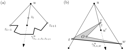
Figure 1: (a) An illustration of the statement of Lemma 10. (b) An example where $u$ is responsible for $t$ and $w$ but not for $v$. The vertex $u^{\prime}$ is responsible for $v$.

A vertex $v$ of a simple polygon $P$ is convex if the internal angle of $P$ at $v$ is less than $\pi$; otherwise $v$ is a reflex vertex of $P$. Let $v$ be a convex vertex of an obstacle $O$ from a minimal obstacle representation $(D,\mathcal{O})$ of $G$ and let $e_{1}$ and $e_{2}$ be the two edges of $O$ adjacent to $v$. Let $T$ be the triangle spanned by the edges $e_{1}$ and $e_{2}$. Assume first that the interior of $T$ does not contain any point of $D$ nor a vertex of an obstacle from $\mathcal{O}$. In this case, we call the vertex $v$ blocking.

Since the representation $(D,\mathcal{O})$ is minimal, there is a line segment $s$ representing a non-edge $e$ of $G$ such that $s$ intersects $e_{1}$ and $e_{2}$. Otherwise, if $O$ has at least 4 vertices, we could remove $v$ and reduce the number of vertices of the obstacles from $\mathcal{O}$. If $s$ does not have any other intersections with obstacles from $\mathcal{O}$, then we say $e$ is forces $v$. Then each blocking vertex of an obstacle with at least 4 vertices is forced by at least one non-edge of $G$.

Let $u$ be an end-vertex of a non-edge $uu^{\prime}$ that forces $v$ and let $z$ be an intersection point of $uu^{\prime}$ with an edge of $\partial O$ incident to $v$. We then say that $u$ is responsible for $v$ if the following situation does not happen: there are non-edges of $G$ containing $u$ and forcing two other vertices $t$ and $w$ of $O$ that span the polygonal chain $\gamma^{u}_{t,z,w}$ from Lemma 10; see Figure 1(b).

We now prove a linear upper bound on the number of blocking vertices of an obstacle. To do so, we need the following auxiliary result.

Lemma 11.

Let $G$ be a graph with a minimal obstacle representation $(D,\mathcal{O})$ and let $v$ be a blocking vertex of some obstacle $O\in\mathcal{O}$ with at least 4 vertices. Then, there is at least one vertex of $G$ that is responsible for $v$.

Proof.

Let $uu^{\prime}$ be a non-edge of $G$ forcing $v$. Let $z$ be an intersection point of $uu^{\prime}$ with an edge of $\partial O$ incident to $v$. Suppose that $u$ is not responsible for $v$. Then, there are two other non-edges $ua$ and $ub$ of $G$ forcing two other vertices $t$ and $w$ of $O$, respectively, such that the polygonal chain $\gamma^{u}_{t,z,w}\subseteq\partial O$ between $t$ and $w$ intersects the ray $\overrightarrow{uz}$ at some point $x\neq z$; see Figure 2(a) for an illustration. Since $v$ is forced by $uu^{\prime}$, the point $x$ lies behind $u^{\prime}$ on the ray $\overrightarrow{uz}$.

We claim that $u^{\prime}$ is responsible for $v$. Suppose for a contradiction that this is not the case. Then, analogously, there are non-edges $ua^{\prime}$ and $ub^{\prime}$ of $G$ forcing two other vertices $t^{\prime}$ and $w^{\prime}$ of $O$, respectively, such that the polygonal chain $\gamma^{u^{\prime}}_{t^{\prime},z,w^{\prime}}\subseteq\partial O$ between $t^{\prime}$ and $w^{\prime}$ intersects the ray $\overrightarrow{u^{\prime}z}$ at some point $x^{\prime}\neq z$. Similarly as before, the point $x^{\prime}$ lies behind $u$ on the ray $\overrightarrow{u^{\prime}z}$.

Since $t$ and $w$ are forced by $ua$ and $ub$, respectively, the vertices $a^{\prime}$ and $b^{\prime}$ lie outside the region $R$ bounded by the line segments $\overline{ut}$, $\overline{uw}$, and by the curve $\gamma^{u}_{t,z,w}$. Otherwise at least one of the segments $ua$ and $ub$ has another intersection with $O$. Analogously, the vertices $a$ and $b$ lie outside the region $R^{\prime}$ bounded by the line segments $\overline{ut^{\prime}}$, $\overline{uw^{\prime}}$, and by the curve $\gamma^{u^{\prime}}_{t^{\prime},z,w^{\prime}}$. Since $z$ lies above $x$ on $\overrightarrow{uz}$ and above $x^{\prime}$ on $\overrightarrow{u^{\prime}z}$, we see $z\in R\cap R^{\prime}$. Thus, $z$ lies in the region bounded by the line segments $\overline{ua}$, $\overline{ub}$, $\overline{ua^{\prime}}$, and $\overline{ub^{\prime}}$. However, the interior of at least one of these line segments has to be intersected by the portion of $\partial O$ between $z$ and, say, $t$. This contradicts the fact that each of these four line segments is forcing a vertex of $O$. ∎

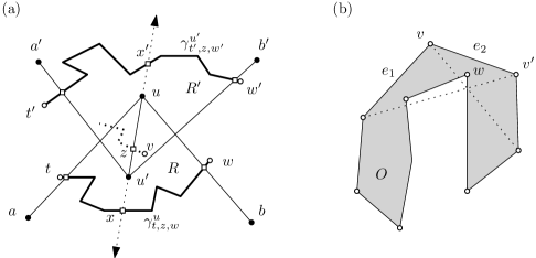
Figure 2: (a) An illustration of the proof of Lemma 11. (b) The reflex vertex $w$ is responsible for the non-blocking convex vertices $v$ and $v^{\prime}$ of the obstacle $O$.

Now, we can use a double-counting argument to show that the number of convex vertices in each obstacle is at most linear in the number of vertices of $G$.

Lemma 12.

Let $O$ be an obstacle from a minimal obstacle representation $(D,\mathcal{O})$ of a connected graph $G$ with $n\geq 2$ vertices. Then $O$ has at most $2n$ blocking vertices.

Proof.

First, we assume that $O$ has at least 4 vertices. Otherwise the statement is trivial as $n\geq 2$. Thus, if a vertex $v$ of $O$ is blocking, the edges of $O$ adjacent to $v$ are intersected by a non-edge of $G$.

Now we show that every vertex of $G$ is responsible for at most two blocking vertices of $O$. Suppose for contradiction that there is a vertex $u$ of $G$ that is responsible for at least three blocking vertices $v_{0}$, $v_{1}$, and $v_{2}$ of $O$. For every $i\in\{0,1,2\}$, let $z_{i}$ be a point of $\partial O$ that lies on a non-edge of $G$ that forces $v_{i}$. By Lemma 10, there is $i\in\{0,1,2\}$ and a polygonal chain $\gamma^{u}_{z_{i-1},z_{i},z_{i+1}}\subseteq\partial O$ between $z_{i-1}$ and $z_{i+1}$ such that $\gamma^{u}_{z_{i-1},z_{i},z_{i+1}}$ intersects the ray $\overrightarrow{uz_{i}}$ at some point different from $z_{i}$ (the indices are taken modulo 3). By the choice of $z_{0},z_{1},z_{2}$, the ray $\overrightarrow{uz_{i}}$ intersects the chain $\gamma^{u}_{v_{i-1},z_{i},v_{i+1}}$ at some point different from $z_{i}$. This contradicts the fact that $u$ is responsible for $v_{i}$, as we have excluded this situation in the definition of responsibility.

We use a double-counting argument on the number $x$ of pairs $(u,v)$, where $u$ is a vertex of $G$ that is responsible for a blocking vertex $v$ of $O$. By Lemma 11, for every blocking vertex $v$ of $O$, there is at least one vertex of $G$ that is responsible for $v$. Thus, $x$ is at least as large as the number of blocking vertices of $O$. On the other hand, since every vertex of $G$ is responsible for at most two blocking vertices of $O$, we have $x\leq 2n$. Altogether, the number of blocking vertices of $O$ is at most $2n$. ∎

We note that the proof of Lemma 12 can be modified to show that each convex obstacle $O$ has at most $n$ vertices. This is because exactly two vertices of $G$ are then responsible for each vertex of $O$ and all vertices of $O$ are blocking.

Now, we consider the remaining convex vertices of obstacles from a minimal obstacle representation $(D,\mathcal{O})$ of $G$. We call such vertices non-blocking.

Lemma 13.

Let $O$ be an obstacle from a minimal obstacle representation $(D,\mathcal{O})$ of a graph $G$ with $n$ vertices. Then $O$ has at most $2r_{O}$ non-blocking vertices where $r_{O}$ is the number of reflex vertices of $O$.

Proof.

Without loss of generality, we assume that no three vertices of obstacles are collinear otherwise we apply a suitable perturbation. Let $v$ be a non-blocking vertex of $O$. Let $T$ be the triangle spanned by the edges $e_{1}$ and $e_{2}$ of $O$ that are incident to $v$. Since $v$ is non-blocking, the interior of $T$ contains either some vertex of $G$ or a vertex of an obstacle from $\mathcal{O}$; see Figure 2(b). Consider the line $\ell$ that contains $v$ and that is orthogonal to the axis of the acute angle between $e_{1}$ and $e_{2}$. We sweep $\ell$ along the axis until, for the first time, the part of $\ell$ in the interior of $T$ meets a point $w$ that is not in the interior of $O$. Then $w$ is a reflex vertex of $O$ since the obstacles are pairwise disjoint and no vertex of $G$ is contained in $O$. We say that $w$ is responsible for $v$.

Now, we show that each reflex vertex of $O$ is responsible for at most two non-blocking vertices of $O$. Let $v$ and $v^{\prime}$ be two non-blocking vertices of $O$ and let $w$ be a reflex vertex of $O$ responsible for $v$ and $v^{\prime}$. Let $T$ be the triangle spanned by the edges of $O$ that are incident to $v$. The only points from $\partial O$ that are in the swept part of $T$ just before we meet $w$ are from $e_{1}$ and $e_{2}$. This claim is also true for the triangle $T^{\prime}$ that is analogously defined for $v^{\prime}$. Thus, since no three vertices of obstacles are collinear, the triangles $T$ and $T^{\prime}$ share an edge. Therefore, $w$ cannot be responsible for more than two such vertices.

We now use a double-counting argument on the number $x$ of pairs $(w,v)$, where $w$ is a reflex vertex of $O$ that is responsible for a non-blocking vertex $v$ of $O$. For every such vertex $v$ of $O$, there is at least one reflex vertex of $O$ that is responsible for $v$. Thus, $x$ is at least as large as the number of non-blocking vertices of $O$. On the other hand, since every reflex vertex of $O$ is responsible for at most two non-blocking vertices of $O$, we have $x\leq 2r_{O}$. Altogether, the number of non-blocking vertices of $O$ is at most $2r_{O}$. ∎

The only remaining vertices of obstacles are the reflex vertices. The following result gives an estimate on their number in a minimal obstacle representation.

Lemma 14.

Let $(D,\mathcal{O})$ be a minimal obstacle representation of a connected graph $G$ with $n$ vertices. Then the total number of reflex vertices of obstacles from $\mathcal{O}$ is at most $2n+5$.

Proof.

Without loss of generality, we assume that no three vertices of obstacles are collinear otherwise we apply a suitable perturbation. Let $v$ be a reflex vertex of an obstacle $O$ from $\mathcal{O}$. We use $e_{1}$ and $e_{2}$ to denote the two edges of $O$ that contain $v$ and $T$ to denote the triangle spanned by $e_{1}$ and $e_{2}$. The interior of $T$ contains some point from $D\cup\bigcup\mathcal{O}$ as otherwise we could remove $v$ by considering a new obstacle $O\cup T$, which is impossible as $(D,\mathcal{O})$ is minimal.

Similarly as in the proof of Lemma 13, we consider the line $\ell$ that contains $v$ and that is orthogonal to the axis of the acute angle between $e_{1}$ and $e_{2}$. We sweep $\ell$ along the axis until the part of $\ell$ in the interior of $T$ meets a point $w$ from $D\cup\bigcup\mathcal{O}$ for the first time. Then $w$ is either some vertex of $D$ or a vertex of some obstacle from $\mathcal{O}$. We distinguish three cases.

First, suppose that $w$ is a vertex of another obstacle $O^{\prime}$ from $\mathcal{O}$. Then we can merge the obstacles $O$ and $O^{\prime}$ by adding a small polygon inside the a small neighborhood of the swept portion of $T$ containing $w$; see Figure 3(a). This, however, is impossible as $(D,\mathcal{O})$ is minimal and, in particular, uses the minimum number of obstacles for $G$.

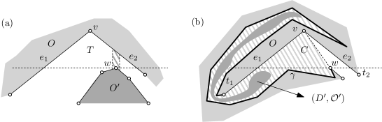
Figure 3: An illustration of the proof of Lemma 14. (a) Merging two obstacles. (b) If $w\in O$, then there is an isolated component $(D^{\prime}\mathcal{O}^{\prime})$ in the region $C$ (denoted by stripes).

Second, assume that $w$ is a vertex of the obstacle $O$. Let $t_{1}$ and $t_{2}$ be the endpoints of $e_{1}$ and $e_{2}$, respectively, different from $v$. Since $O$ is a simple polygon, there is a polygonal chain $\gamma\subseteq\partial O$ between $w$ and some $t_{i}$ enclosing together with line segments $e_{i}$ and $\overline{vw}$ a region $C$ such that $C$ does not contain $t_{3-i}$; see Figure 3(b). By symmetry, we assume $i=1$. Let $D^{\prime}=D\cap C$ and $\mathcal{O}^{\prime}$ be the set of obstacles from $\mathcal{O}$ that are contained in $C$. Note that $(D^{\prime},\mathcal{O}^{\prime})=(D,\mathcal{O}\setminus\{O\})$ as $G$ is connected and $(D^{\prime},\mathcal{O}^{\prime})$ is an obstacle representation of a subgraph of $G$ that is isolated from everything outside of $C$, since every line segment connecting a point of $D^{\prime}$ with a point from $D\setminus D^{\prime}$ intersects $O$. We say that that the edge $vw$ is a cutting segment bounding $C$.

We show that there are at most five reflex vertices that are endpoints of cutting segments. Suppose for contradiction that we have cutting segments $v_{1}w_{1},\dots,v_{m}w_{m}$ bounding regions $C_{1},\dots,C_{m}$, respectively, where $m\geq 6$ and $v_{1},\dots,v_{m}$ are distinct. Then all the cutting segments have endpoints in the same obstacle $O$, for every $i\in[m]$, as the drawing $D$ has $O_{i}$ in the outerface, which cannot contain any other obstacle as otherwise we could merge them, contradicting the minimality of $(D,\mathcal{O})$. The line segments $v_{1}w_{1},\dots,v_{m}w_{m}$ do not cross as, after possible relabeling, we have $C_{1}\supset\dots\supset C_{m}$ and $v_{i}w_{i}$ is contained in $\partial C_{i}$ for every $i\in[m]$; see Figure 4. For each $i\in[m-1]$, let $C^{\prime}_{i}=C_{i}\setminus C_{i+1}$. It follows from the definition of cutting segments that the regions $C^{\prime}_{1},\dots,C^{\prime}_{m-1}$ do not contain any point of $D$ nor a point of an obstacle from $\mathcal{O}$ in their interior. We now reduce the number of vertices of $O$. The set $O\cup C^{\prime}_{1}\cup\dots\cup C^{\prime}_{m-1}$ is a polygon with a single hole corresponding to the region $C_{m}$. Let $t$ be a point of $C_{m}$ with the smallest $y$-coordinate and note that we can assume that $t$ is a vertex of $O$. Let $s\subseteq O$ be a vertical line segment with the topmost point $t$. By the choice of $t$, the other endpoint of $s$ is a point from $\partial O$ that does not lie in $\partial C_{m}$. Thus, we can replace $O$ with a new obstacle $O^{\prime}$ obtained from $O\cup C^{\prime}_{1}\cup\dots\cup C^{\prime}_{m-1}$ by removing a small rectangular neighborhood of $s$; see Figure 4. Since $t$ is a vertex of $O$, we add at most three new vertices to $O^{\prime}$ with respect to $O$. On the other hand, we remove at least $m-2\geq 4$ vertices, as $v_{2},\dots,v_{m-1}$ will no longer be vertices of $O^{\prime}$. This contradicts the minimality of $(D,\mathcal{O})$.

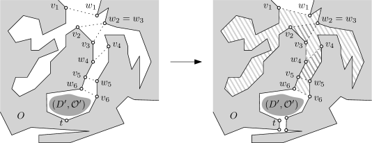
Figure 4: An illustration of the proof of Lemma 14. Reducing the number of vertices of an obstacle $O$ by filling up regions $C^{\prime}_{1},\dots,C^{\prime}_{5}$ and “drilling” a vertical tunnel from the vertex $t$ of $C_{6}$.

Finally, assume that $w$ is a vertex of $G$. Then we say that $w$ is responsible for $v$. We now show that every vertex of $G$ is responsible for at most two reflex vertices of an obstacle. This is done via a similar argument as in the proof of Lemma 13. Let $v$ and $v^{\prime}$ be two reflex vertices of some obstacles $O$ and $O^{\prime}$, respectively, and let $w$ be a vertex of $G$ responsible for $v$ and $v^{\prime}$. Let $T$ be the triangle spanned by the edges $e_{1}$ and $e_{2}$ of $O$ that are incident to $v$. The only points from any obstacle that are in the swept part of $T$ just before we meet $w$ are from $e_{1}$ and $e_{2}$. This claim is true for the triangle $T^{\prime}$ that is defined analogously for $v^{\prime}$. Thus, since no three vertices of obstacles are collinear, the triangles $T$ and $T^{\prime}$ share an edge. Therefore, $w$ cannot be responsible for more than two reflex vertices.

Now, every vertex of $G$ is responsible for at most two reflex vertices in total. Thus, since apart for at most 5 endpoints of cutting segments for each reflex vertex $v$ of an obstacle there is at least one vertex of $G$ that is responsible for $v$, we get that the total number of reflex vertices is at most $2n+5$. ∎

To bound the number $g(h,n)$ of connected $n$-vertex graphs with obstacle number at most $h$, we follow the approach by Mukkamala, Pach, and Pálvölgyi [17], which is based on encoding point sets by order types. Let $P$ and $Q$ be two sets of points in the plane in general position. Then, $P$ and $Q$ have the same order type if there is a one-to-one correspondence between them with the property that the orientation of any triple of points from $P$ is the same as the orientation of the corresponding triple of points from $Q$. Recall that we consider only point sets in general position so the orientation is either clockwise or counterclockwise. So, formally, an order type of a set $P$ of points in the plane in general position is a mapping $\chi$ that assigns $\chi(a,b,c)\in\{+1,-1\}$ to each ordered triple $(a,b,c)$ of points from $P$, indicating whether $a,b,c$ make a left turn (+1) or a right turn (-1).

We use the following classical estimates by Goodman and Pollack [13, 14] on the number of order types of sets of $n$ points.

Theorem 15 ([13, 14]).

The number of order types on $n$ labeled points in $\mathds{R}^{2}$ is at most $\left(\frac{n}{2}\right)^{4(1+o(1))n}\in 2^{O(n\log n)}$.

Now, for each connected $n$-vertex graph $G$ with obstacle number at most $h$, fix a minimal obstacle representation $(D,\mathcal{O})$ of $G$ with $|\mathcal{O}|\leq h$. Let $s$ be the number of vertices of obstacles from $\mathcal{O}$ and let $r_{O}$ be the number of reflex vertices of an obstacle $O$ from $\mathcal{O}$. We use $r$ to denote the total number of reflex vertices $\sum_{O\in\mathcal{O}}r_{O}$. Since every vertex of an obstacle is either convex (blocking or non-blocking) or reflex, Lemmas 12, 13, and 14 give

$$s\leq r+\sum_{O\in\mathcal{O}}(2r_{O}+2n)\leq 3r+|\mathcal{O}|\cdot 2n\leq 2hn+6n+15.$$

Let $S$ be a sequence of $n+s$ labeled points starting with the vertices of $G$ and followed by the vertices of the obstacles (listed one by one, in cyclic order, and properly separated from one another). Then, the order type of $S$ determines the graph $G$ as it stores all the information about incidences in the obstacle representation $(D,\mathcal{O})$. By Theorem 15, the number of such order types is at most $2^{\alpha(n+s)\log{(n+s)}}$ for some suitable constant $\alpha>0$. Since $s\leq 2hn+6n+15$ and $h\leq\binom{n}{2}$, we obtain the desired upper bound

$$g(h,n)\in 2^{\alpha(n+2hn+6n+15)\log{(n+2hn+6n+15)}}\subseteq 2^{O(hn\log{n})}.$$

3.2 Proof of Theorem 4

We show that the number of graphs on $n$ vertices that have convex obstacle number at most $h$ is bounded from above by $2^{O(n(h+\log n))}$. That is, we prove the bound $f_{\mathrm{c}}(h,n)\in 2^{O(n(h+\log n))}$, which improves the earlier estimate $f_{\mathrm{c}}(h,n)\in 2^{O(hn\log{n})}$ by Mukkamala, Pach, and Pálvölgyi [17] and for $h<n$ asymptotically matches the lower bounds by Balko, Cibulka, and Valtr [3].

To this end, we find an efficient encoding of an obstacle representation $(D,\mathcal{O})$ for any $n$-vertex graph $G=(V,E)$ that uses at most $h$ convex obstacles. We identify the vertex set $V$ and the points of $D$ that represent the vertices from $V$. The first part of the encoding is formed by the order type of $V$. By Theorem 15, there are at most $2^{O(n\log{n})}$ order types of sets of $n$ points in the plane in general position.

It remains to encode the obstacles and their interaction with the line segments between points from $V$. To do that, we use so-called radial systems. The clockwise radial system $R$ of $V$ assigns to each vertex $v\in V$ the clockwise cyclic ordering $R(v)$ of the $n-1$ rays in $D$ that start from $v$ and pass through a vertex from $V\setminus\{v\}$. The order type of $V$ uniquely determines the radial system $R$ of $V$. Essentially, this also holds in the other direction: There are at most $n-1$ order types that are compatible with a given radial system [1].

For a vertex $v\in V$ and an obstacle $O\in\mathcal{O}$, let $I_{O}(v)$ be the subsequence of rays in $R(v)$ that intersect $O$. We say that a subset $I$ of $R(v)$ is an interval if there are no four consecutive elements $a,b,c,d$ in the radial order $R(v)$ such that $a,c\in I$ and $b,d\notin I$. Since $O$ is connected, we get the following result.

Observation 16.

For every vertex $v\in V$ and each obstacle $O\in\mathcal{O}$, the set $I_{O}(v)$ forms an interval in the radial ordering $R(v)$. ∎

Thus, we call the set $I_{O}(v)$ the blocking interval of the pair $(v,O)$. For convex obstacles, knowing which rays from a vertex towards other vertices are blocked by an obstacle suffices to know which edges are blocked by this obstacle.

Lemma 17.

For two vertices $u,v\in V$, the pair $\{u,v\}$ is a non-edge of $G$ if and only if there is an obstacle $O\in\mathcal{O}$ such that $u\in I_{O}(v)$ and $v\in I_{O}(u)$.

Proof.

Consider two vertices $u,v\in V$. Let $R_{u}$ be the ray starting at $u$ and passing through $v$ and let $R_{v}$ be the ray starting at $v$ and passing through $u$. Then $uv=R_{u}\cap R_{v}$. Since each obstacle $O\in\mathcal{O}$ is convex, the intersection of $O$ with each ray or line segment is a (possibly empty) line segment. Thus, $O$ intersects both rays $R_{u}$ and $R_{v}$ if and only if $O$ intersects the line segment $\overline{uv}$. Since $(D,\mathcal{O})$ is an obstacle representation of $G$, we then have $\{u,v\}\notin E$ if and only if $u\in I_{O}(v)$ and $v\in I_{O}(u)$. ∎

We note that Lemma 17 is not true if the obstacles from $\mathcal{O}$ are not convex, since both rays $R_{u}$ and $R_{v}$ could then be blocked although the line segment $\overline{uv}$ is not.

By Observation 16 and Lemma 17, it suffices to encode the blocking intervals $I_{O}(v)$ for every $v\in V$ and $O\in\mathcal{O}$. In the following we will describe how to obtain an encoding of size $2^{O(hn)}$ for the blocking intervals, which together with the order type of $V$ yields the claimed bound on $f_{c}(h,n)$. In order to describe our approach, it is more convenient to move to the dual setting, using the standard projective duality transformation that maps a point $p=(p_{x},p_{y})\in\mathds{R}^{2}$ to the line $p^{*}=\{(x,y)\in\mathds{R}^{2}\colon y=p_{x}x-p_{y}\}$, and that maps a non-vertical line $\ell=\{(x,y)\in\mathds{R}^{2}\colon y=mx+b\}$ to the point $\ell^{*}=(m,-b)$. This map is an involution, that is, $(p^{*})^{*}=p$ and $(\ell^{*})^{*}=\ell$. Moreover, it preserves incidences, that is, $p\in\ell\Longleftrightarrow\ell^{*}\in p^{*}$, and is order-preserving as a point $p$ lies above $\ell\Longleftrightarrow\ell^{*}$ lies above $p^{*}$.

So consider the arrangement $\mathcal{A}$ of the set $V^{*}$ of $n$ lines dual to the points in $V$. Note that the combinatorial structure of $\mathcal{A}$ itself, that is, the sequences of intersections with other lines along each line, can be obtained from the radial system of $V$, cf. [22]. (To be able to identify the vertical direction and the $x$-order of the vertices, we add a special point very high above all other points.) Let $O$ be an obstacle from $\mathcal{O}$. Define a map $\tau$ that assigns to each $x\in\mathds{R}$ the upper tangent of slope $x$ to $O$, that is, the line $\tau(x)$ of slope $x$ that is tangent to $O$ and such that $O$ lies below $\tau(x)$; see Figure 5 for an illustration. Now, consider the dual $\tau^{*}$ of $\tau$, defined by $\tau^{*}(x)=(\tau(x))^{*}$. Note that, by definition, every line in the image of $\mathds{R}$ via $\tau$ passes through a vertex of the upper envelope $O^{+}$ of the convex hull of $O$. Consequently, each point $\tau^{*}(x)$ lies on a line that is dual to a vertex of $O^{+}$. In other words, $\tau^{*}$ is a piecewise linear function that is composed of line segments along the lines dual to the vertices of $O^{+}$. The order of these line segments from left to right (in increasing $x$-order) corresponds to primal tangents of increasing slope and, therefore, to the order of the corresponding vertices of $O^{+}$ from right to left (in decreasing $x$-order). As primal $x$-coordinates correspond to dual slopes, the slopes of the line segments along $\tau^{*}$ monotonically decrease from left to right, and so $\tau^{*}$ is concave.

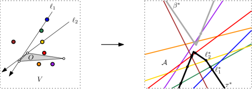
Figure 5: An example of a vertex set $V$ with its dual line arrangement $\mathcal{A}=V^{*}$. Points and lines of the same color are dual to each other. The curve $\tau^{*}$ for the upper envelope $O^{+}$ of the obstacle $O$ is denoted black and the curve $\beta^{*}$ for the lower envelope $O^{-}$ of the obstacle $O$ is denoted gray.

The primal line of a point in $v^{*}\cap\tau^{*}$, for some $v\in V$, passes through $v$ and is an upper tangent to $O$. So such an intersection corresponds to an endpoint of the blocking interval $I_{O}(v)$. In order to obtain all endpoints of the blocking interval $I_{O}(v)$, we eventually also consider the lower tangents to $O$ in an analogous manner. The corresponding function $\beta^{*}$ is convex and consists of segments along lines dual to the vertices of the lower convex hull of $O$, in increasing $x$-order.

It remains to describe how to compactly encode the intersections of $\tau^{*}$ with $\mathcal{A}$. To do so, we apply a result by Knuth [16]; see also the description by Felsner and Valtr [8]. A set $\mathcal{A^{\prime}}$ of biinfinite curves in $\mathds{R}^{2}$ forms an arrangement of pseudolines if each pair of curves from $\mathcal{A}^{\prime}$ intersects in a unique point, which corresponds to a proper, transversal crossing. A curve $\alpha$ is a pseudoline with respect to $\mathcal{A^{\prime}}$ if $\alpha$ intersects each curve in $\mathcal{A^{\prime}}$ at most once. Let $\gamma$ be a curve that intersects each curve from $\mathcal{A}^{\prime}$ in a finite number of points. The cutpath of $\gamma$ in $\mathcal{A^{\prime}}$ is the sequence of intersections of $\gamma$ with the pseudolines from $\mathcal{A^{\prime}}$ along $\gamma$.

Theorem 18 ([16]).

If $\alpha$ is a pseudoline with respect to an arrangement $\mathcal{A^{\prime}}$ of $n$ pseudolines, then there are at most $O(3^{n})$ cutpaths of $\alpha$ in $\mathcal{A^{\prime}}$.

Using Theorem 18, we can now estimate the number of cutpaths of $\tau^{*}$ with respect to $\mathcal{A}$.

Lemma 19.

There are $O(216^{n})$ cutpaths of $\tau^{*}$ in $\mathcal{A}$.

Proof.

If $\tau^{*}$ was a pseudoline with respect to $\mathcal{A}$, then using Theorem 18 we could conclude that there are only $O(3^{n})$ cutpaths of $\tau^{*}$ in $\mathcal{A}$. However, $\tau^{*}$ is not a pseudoline with respect to $\mathcal{A}$ in general because a vertex from $V$ can be contained in two tangents to $O^{+}$, in which case $\tau^{*}$ intersects the corresponding line of $\mathcal{A}$ twice. More precisely, this is the case exactly for those points from $V$ that lie vertically above $O$, whereas all points that lie to the left or to the right of $O$ have only one tangent to $O^{+}$ and one tangent to the lower envelope $O^{-}$ of the convex hull of $O$. All points that lie vertically below $O$ have no tangent to $O^{+}$ but two tangents to $O^{-}$. (We assign the tangents to the leftmost and rightmost vertex of $O$ as we see fit.)

To remedy this situation, we split the lines of $\mathcal{A}$ into two groups: Let $\mathcal{A}_{1}$ denote the arrangement of those lines from $\mathcal{A}$ that intersect $\tau^{*}$ at most once, and let $\mathcal{A}_{2}$ denote the arrangement of those lines from $\mathcal{A}$ that intersect $\tau^{*}$ exactly twice. To describe a cutpath of $\tau^{*}$ in $\mathcal{A}$ it suffices to encode (1) which lines are in $\mathcal{A}_{1}$; (2) the cutpath of $\tau^{*}$ in $\mathcal{A}_{1}$; (3) the cutpath of $\tau^{*}$ in $\mathcal{A}_{2}$; and (4) a bitstring that tells us whether the next crossing is with a line from $\mathcal{A}_{1}$ or from $\mathcal{A}_{2}$ when walking along $\tau^{*}$ from left to right. For (1) there are $2^{n}$ options, for (2) there are $O(3^{n})$ options by Theorem 18, and for (4) there are at most $2^{2n}=4^{n}$ options. It remains to argue how to encode (3).

To encode the cutpath of $\tau^{*}$ in $\mathcal{A}_{2}$, we split each line $\ell\in\mathcal{A}_{2}$ at its leftmost crossing $\mathrm{c}_{\ell}$ with $\tau^{*}$ and construct a pseudoline $\ell^{\prime}$ by taking the part of $\ell$ to the left of $\mathrm{c}_{\ell}$ and extending it to the right by an almost vertical downward ray (that is, so that no vertex of $\mathcal{A}$ lies between the vertical downward ray from $\mathrm{c}_{\ell}$ and $\ell^{\prime}$). Now the collection $\{\ell^{\prime}\colon\ell\in\mathcal{A}_{2}\}$ induces a pseudoline arrangement $\mathcal{A}_{2}^{\prime}$ such that $\tau^{*}$ is a pseudoline with respect to $\mathcal{A}_{2}^{\prime}$. Note that $\tau^{*}$ crosses all pseudolines in $\mathcal{A}_{2}^{\prime}$ from below. We claim that the cutpath of $\tau^{*}$ in $\mathcal{A}_{2}^{\prime}$ together with $\mathcal{A}_{2}$ suffices to reconstruct $\mathcal{A}_{2}^{\prime}$.

Let us prove this claim. So suppose we are given $\mathcal{A}_{2}$ and the cutpath $p$ of $\tau^{*}$ in $\mathcal{A}_{2}^{\prime}$. The cutpath $p$ is encoded as a bitstring that determines if the path continues by leaving the current cell through its leftmost or rightmost edge and the set of lines that is crossed as a middle (i.e., neither leftmost nor rightmost) edge of a cell as soon as it is encountered in such a way. This information suffices to decribe $p$ because it can be shown that $p$ encounters every line of $\mathcal{A}_{2}^{\prime}$ at most once as a middle edge of a cell, cf. [8, 16].

To recover $\mathcal{A}_{2}^{\prime}$ we trace $p$ from left to right. We know that the starting cell of $p$ in $\mathcal{A}_{2}$ is the bottom cell of $\mathcal{A}_{2}$. Then we just proceed by pretending that $p$ was described with respect to $\mathcal{A}_{2}$. However, at each crossing we cut the line $\ell$ crossed by $p$ and discard the part of $\ell$ to the right of the crossing and replace it by an almost vertical downward ray, as described above in the construction of $\mathcal{A}_{2}^{\prime}$. Hence, as $p$ crosses only lines that approach it from above, no line whose leftmost crossing with $p$ has already been processed is ever considered again. Moreover, as we trace $p$ from left to right, whenever a crossing of a line $\ell$ with $p$ is processed, it is the leftmost crossing of $\ell$ with $p$. In other words, all crossings that are discovered during the trace correspond to crossings of $p$ in $\mathcal{A}_{2}^{\prime}$.

Finally, we claim that during the trace $p$ encounters every line at most once as a middle edge of a cell, and so the middle set information (which has been created with respect to $\mathcal{A}_{2}^{\prime}$, but we interpret it in our work in progress arrangement, which is a combination of $\mathcal{A}_{2}$ and $\mathcal{A}_{2}^{\prime}$) suffices for the reconstruction. To see this, suppose that during our trace of $p$ a line $\ell$ is encountered as a middle edge of a cell $C$ and then later again as a middle edge of a cell $C^{\prime}$. Let $\ell^{-}$ be the line that contributes the leftmost edge to the upper boundary of $C^{\prime}$. Then the unique crossing of $\ell^{-}$ and $\ell$ lies to the right of or on $\ell^{\prime}\cap C^{\prime}$ along $\ell^{\prime}$ and $\ell^{\prime}$ lies below $\ell$ to the left of $C^{\prime}$. Further, we know that $\ell^{-}$ does not cross the part of $p$ traced so far (i.e., to the left of $C^{\prime}$) because if it did, we would have cut $\ell^{\prime}$ at this crossing. It follows that to the left of $C^{\prime}$ the pseudolines $p$ and $\ell$ are separated by $\ell^{\prime}$ and so $\ell$ cannot appear on the boundary of any cell $C$ traced by $p$ so far, a contradiction. So, as claimed, during the trace $p$ encounters every line at most once as a middle edge of a cell. This also completes the proof of our claim that the cutpath of $\tau^{*}$ in $\mathcal{A}_{2}^{\prime}$ together with $\mathcal{A}_{2}$ suffices to reconstruct $\mathcal{A}_{2}^{\prime}$.

In a symmetric fashion (vertical flip of the plane) we obtain an arrangement $\mathcal{A}_{2}^{\prime\prime}$ and cutpath to describe the rightmost crossings of the lines in $\mathcal{A}_{2}$ with $\tau^{*}$. Combining both we can reconstruct the cutpath of $\tau^{*}$ in $\mathcal{A}_{2}$. By Theorem 18 there are $O(3^{n})$ options for each of the two cutpaths. So there are $O(9^{n})$ options for (3) and altogether $O(216^{n})$ cutpaths of $\tau^{*}$ in $\mathcal{A}$. ∎

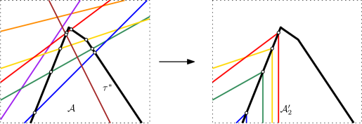
Figure 6: Cutting the lines of $\mathcal{A}$ that cross $\tau^{*}$ twice at their leftmost crossing with $\tau^{*}$. Then $\tau^{*}$ is a pseudoline with respect to the resulting pseudoline arrangement $\mathcal{A}_{2}^{\prime}$.

To summarize, we encode the obstacle representation $(D,\mathcal{O})$ of $G$ by first encoding the order type of $V$. By Theorem 15, there are at most $2^{O(n\log{n})}$ choices for the order type of a set of $n$ points. The order type of $V$ determines the arrangement $\mathcal{A}$ of $n$ lines that are dual to the points from $V$. By Observation 16 and Lemma 17, it suffices to encode the endpoints of the blocking intervals $I_{O}(v)$ for every $v\in V$ and $O\in\mathcal{O}$, which are defined using the radial system of $V$ that is also determined by the order type of $V$. For each obstacle $O\in\mathcal{O}$, the endpoints of all the intervals $I_{V}(O)$ are determined by the cutpath of the curve $\tau^{*}$ in $\mathcal{A}$ constructed for the upper tangents of $O$ and the analogous curve $\beta^{*}$ constructed for the lower tangents of $O$. By Lemma 19, there are at most $O(216^{n})$ cutpaths of $\tau^{*}$ in $\mathcal{A}$ and the same estimate holds for $\beta^{*}$. This gives at most $O((216^{n})^{2})$ possible ways how to encode a single obstacle. Altogether, we thus obtain

$$f_{\mathrm{c}}(h,n)\in 2^{O(n\log{n})}\cdot O(216^{2hn})\subseteq 2^{O(n\log{n}+hn)},$$

which concludes the proof of Theorem 4.

Remark.

It is natural to wonder whether we cannot use Theorem 4 to obtain a linear lower bound on $\operatorname{obs}(n)$ by splitting each obstacle in an obstacle representation $(D,\mathcal{O})$ of a graph $G$ with $|\mathcal{O}|=h$ into few convex pieces and apply Theorem 4 on the resulting obstacle representation $(D,\mathcal{O}^{\prime})$ of $G$ with convex obstacles. But an obstacle $O$ with $r_{O}$ reflex vertices may require splitting into $\Omega(r_{O})$ convex pieces and therefore we may have $|\mathcal{O}^{\prime}|\in\Omega(h+r)$ where $r$ is the total number of reflex vertices of obstacles in $\mathcal{O}$. Unfortunately, $r$ can be linear in $n$ and then the resulting bound $2^{O(n\log{n}+(h+r)n)}$ may be larger then the number $2^{\binom{n}{2}}$ of $n$-vertex graphs, in which case the proof of Theorem 2 from Section 2 no longer works.

4 A Lower Bound on the Obstacle Number of Drawings

Here, we prove Theorem 6 by showing that there is a constant $\delta>0$ such that, for every $n$, there exists a graph $G$ on $n$ vertices and a drawing $D$ of $G$ such that ${\rm obs}(D)\geq\delta\cdot n^{2}$. The proof is constructive. We first assume that $n$ is even.

A set of points in the plane is a cup if all its points lie on the graph of a convex function. Similarly, a set of points is a cap if all its points lie on the graph of a concave function. For an integer $k\geq 3$, a convex polygon $P$ is $k$-cap free if no $k$ vertices of $P$ form a cap of size $k$. Note that $P$ is $k$-cap free if and only if it is bounded from above by at most $k-2$ segments (edges of $P$). We use $e(P)$ to denote the leftmost edge bounding $P$ from above; see Figure 7(a).

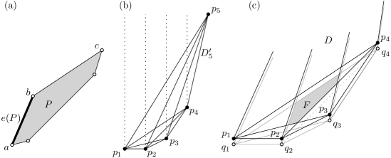
Figure 7: (a) A 4-cap free polygon $P$ that is not 3-cap free. (b) An example of the drawing $D^{\prime}_{m}$ for $m=5$. If the point $p_{m}$ is chosen sufficiently high above $C_{m-1}$, then each line segment $\overline{p_{i}p_{m}}$ with $i<m$ is very close to the vertical line containing $p_{i}$ and thus all faces of $D^{\prime}_{m}$ will be 4-cap free. (c) An example of a part of the drawing $D$ with an example of a face $F$ of $D$. The line segments that are not in $D^{\prime}_{m}$ are drawn grey and the non-edge from $X$ is dotted.

Let $m=n/2$. First, we inductively construct a set $C_{m}$ of $m$ points $p_{1},\dots,p_{m}$ in the plane that form a cup and their $x$-coordinates satisfy $x(p_{i})=i$. We let $C_{1}=\{(1,0)\}$ and $C_{2}=\{(1,0),(2,0)\}$. Now, assume that we have already constructed a set $C_{m-1}=\{p_{1},\dots,p_{m-1}\}$ for some $m\geq 3$. Let $D^{\prime}_{m-1}$ be the drawing of the complete graph with vertices $p_{1},\dots,p_{m-1}$. We choose a sufficiently large number $y_{m}$, and we let $p_{m}$ be the point $(m,y_{m})$ and $C_{m}=C_{m-1}\cup\{p_{m}\}$. We also let $D^{\prime}_{m}$ be the drawing of the complete graph with vertices $p_{1},\dots,p_{m}$. The number $y_{m}$ is chosen large enough so that the following three conditions are satisfied:

1. for every $i=1,\dots,m-1$, every intersection point of two line segments spanned by points of $C_{m-1}$ lies on the left side of the line $\overline{p_{i}p_{m}}$ if and only if it lies to the left of the vertical line $x=i$ containing the point $p_{i}$,

2. if $F$ is a 4-cap free face of $D^{\prime}_{m}$ that is not 3-cap free, then there is no point $p_{i}$ below the (relative) interior of $e(F)$,

3. no crossing of two edges of $D^{\prime}_{m}$ lies on the vertical line containing some point $p_{i}$.

Note that choosing the point $p_{m}$ is indeed possible as choosing a sufficiently large $y$-coordinate $y_{m}$ of $p_{m}$ ensures that for each $i$, all the intersections of the line segments $p_{i}p_{m}$ with line segments of $D^{\prime}_{m-1}$ lie very close to the vertical line $x=i$ containing the point $p_{i}$. Note that it follows from the construction that no line segment of $D^{\prime}_{m}$ is vertical and that no point is an interior point of more than two line segments of $D^{\prime}_{m}$. The drawing $D^{\prime}_{m}$ also satisfies the following claim.

Claim 1.

Each inner face of $D^{\prime}_{m}$ is a 4-cap free convex polygon.

Proof.

We prove the claim by induction on $m$. The statement is trivial for $m\leq 3$ so assume $m\geq 4$. Now, let $F$ be an inner face of $D^{\prime}_{m-1}$. By the induction hypothesis, $F$ is a 4-cap free convex polygon. If $F$ is 3-cap free, then, by the choice of $p_{m}$, the line segments $\overline{p_{i}p_{m}}$ split $F$ into 4-cap free polygons (with the leftmost one being actually 3-cap free); see Figure 7(b). If $F$ is 4-cap free and not $3$-cap free, then the choice of $p_{m}$ guarantees that the line segments $\overline{p_{i}p_{m}}$ split $F$ into 4-cap free polygons. This is because the leftmost such polygon contains the whole edge $e(F)$ as there is no $p_{i}$ below the edge $e(F)$. It remains to consider the inner faces of $D^{\prime}_{m}$ which lie outside of the convex hull of the points $p_{1},\dots,p_{m-1}$. These faces lie inside the triangle $p_{1}p_{m-1}p_{m}$. They are all triangular and therefore satisfy the claim; see the three faces with the topmost vertex $p_{m}=p_{5}$ in Figure 7(b). ∎

For a (small) $\varepsilon>0$ and every $i=1,\dots,m=n/2$, we let $q_{i}$ be the point $(i,y_{i}-\varepsilon)$. That is, $q_{i}$ is a point slightly below $p_{i}$. We choose $\varepsilon$ sufficiently small so that decreasing $\varepsilon$ to any smaller positive real number does not change the combinatorial structure of the intersections of the line segments spanned by the $n$ points $p_{1},\dots,p_{m},q_{1},\dots,q_{m}$. We let $D=D_{n}$ be the drawing with $n$ vertices $p_{1},\dots,p_{m},q_{1},\dots,q_{m}$ containing all the line segments between two vertices, except the line segments $\overline{q_{i}q_{j}}$ where $i$ and $j$ are both even.

We have to show that at least quadratically many obstacles are needed to block all non-edges of $G$ in $D$. Let $X$ be the set of line segments $\overline{q_{i}q_{j}}$ where both $i$ and $j$ are even. Note that each line segment from $X$ corresponds to a non-edge of $G$ and that $|X|=\binom{\lfloor n/4\rfloor}{2}\geq n^{2}/40$ for a sufficiently large $n$.

Claim 2.

Every face of $D$ is intersected by at most two line segments from $X$.

Proof.

The outer face of $D$ is intersected by no line segment of $X$. Every inner face of $D$ is contained in some inner face of $D^{\prime}_{m}$ or in one of the parallelograms $q_{i}q_{i+1}p_{i+1}p_{i}$.

First, suppose that a face $F$ of $D$ is contained in some face $F^{\prime}$ of $D^{\prime}_{m}$. Due to the choice of $\varepsilon$, a line segment $\overline{q_{i}q_{j}}$ of $X$ intersects $F^{\prime}$ (if and) only if a part of the edge $\overline{p_{i}p_{j}}$ bounds $F^{\prime}$ from above. By Claim 1, at most two line segments bound $F^{\prime}$ from above. We conclude that at most two line segments of $X$ intersect $F^{\prime}$. Consequently, also at most two line segments of $X$ intersect $F$.

Suppose now that a face $F$ of $D$ is contained in some parallelogram $Z=q_{i}q_{i+1}p_{i+1}p_{i}$. Let $j$ be the even integer which is equal to $i$ or to $i+1$. Due to the construction, all line segments of $X$ intersecting $Z$ are incident to $q_{j}$. Since edges of $G$ and line segments of $X$ incident to $q_{j}$ alternate around $q_{j}$, at most one line segment of $X$ intersects $F$. ∎

Now, let $\mathcal{O}$ be a set of obstacles such that $D$ and $\mathcal{O}$ form an obstacle representation of $G$. Then each non-edge of $G$ corresponds to a line segment between vertices of $D$ that is intersected by some obstacle from $\mathcal{O}$. In particular, each line segment from $X$ has to be intersected by some obstacle from $\mathcal{O}$. Each obstacle $O$ from $\mathcal{O}$ lies in some face $F_{O}$ of $D$ as it cannot intersect an edge of $G$. Thus, $O$ can intersect only line segments from $X$ that intersect $F_{O}$. It follows from Claim 2 that each obstacle from $\mathcal{O}$ intersects at most two line segments from $X$. Since $|X|\geq n^{2}/40$, we obtain $|\mathcal{O}|\geq|X|/2\geq n^{2}/80$. Consequently, ${\rm obs}(D)\geq n^{2}/80$, which finishes the proof for $n$ even. If $n$ is odd, we use the above construction for $n-1$ and add an isolated vertex to it.

5 Obstacle Number is FPT Parameterized by Vertex Cover Number

In this section we show that computing the obstacle number is fixed-parameter tractabile with respect to the vertex cover number. As our first step towards a fixed-parameter algorithm, we show that, for every graph, its obstacle number is upper-bounded by a function of its vertex cover number.

Lemma 20.

Let $G$ be a graph with vertex cover number $k$. Then $G$ admits an obstacle representation with $1+\binom{k}{2}+k\cdot 2^{k}$ obstacles.

Proof.

Our proof is by construction. Let $X\subseteq V$ be a cardinality-$k$ vertex cover of $G=(V,E)$. We begin by placing the vertices in $X$ on an arc $\gamma$ that is a small part of a circle with some center $c$. For an example, see Figure 8, where $X=\{x,y,z\}$. This ensures that $X$ is in general position. For each pair of non-adjacent vertices $x,y\in X$, we then place a single “tiny” point-like obstacle in the immediate vicinity of either $x$ or $y$; the choice is arbitrary. Crucially, these at most $\binom{k}{2}$ many obstacles will not obstruct any visibility between other pairs of vertices in $G$. (In Figure 8, these are the two square obstacles.)

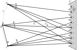
Figure 8: The obstacle number is bounded by a function of the vertex cover number.

Next, we partition the vertices in $V\setminus X$ into at most $2^{k}$ equivalence classes called types based on the following equivalence: two vertices $a,b\in V\setminus X$ have the same type if and only if they have the same neighborhood. We place these vertices on a line $\ell$ sufficiently far from $\gamma$. On this line, we mark $2^{k}$ sufficiently small, pairwise disjoint segments—one for each type. We place $\ell$ orthogonally to the line $\ell^{\prime}$ that connects the center of $\gamma$ to $c$. The small segments will be placed in the general vicinity of the intersection point of $\ell$ and $\ell^{\prime}$. The idea is that the vertices of some type will all be placed on the segment of $\ell$ dedicated to that type. (In Figure 8, there is only one representative of each type.)

We now construct a single obstacle $Q$ that blocks the pairwise visibilities between all vertices placed on $\ell$; see Figure 8. The boundary of $Q$ consists of a zig-zag line whose zigs and zags all intersect $\ell$ and whose first and last line segments are a bit longer than the others. We close $Q$ by connecting the endpoints of the zig-zag line by a line segment that is parallel to $\ell$. Intuitively, the shape of $Q$ can be described as a “hair comb”. By construction, $Q$ guarantees that no two vertices placed on $\ell$ will be visible to each other. At the same time, $Q$ does not obstruct visibilities between the vertices in $X$ and those in $V\setminus X$.

To complete the construction, it suffices to block the visibilities between the vertices in the types and the vertices in $X$. To this end, for each type $T\subseteq V\setminus X$ and each vertex $x\in X$ such that no vertex in $T$ is adjacent to $x$, we add a single nearly point-like obstacle in the immediate vicinity of $x$ that (i) blocks visibility between $x$ and the line segment of $\ell$ dedicated to $T$, but (ii) does not block visibility between any other pair of vertices in the construction. (In Figure 8, these are the triangular obstacles.) To see that this is possible, observe that, since $\gamma$ is a circular arc, small obstacles can be placed in the immediate vicinity of vertices on $\gamma$ in the direction of $c$ without lying on lines connecting other vertices on $\gamma$.

This completes the construction. We have used at most $1+\binom{k}{2}+k\cdot 2^{k}$ obstacles. ∎

Our algorithm crucially uses the exponential-time decision procedure for the existential theory of the reals (ETR) by Renegar [19, 20, 21]. An existential first-order formula about the reals is a formula of the form $\exists x_{1}\dots\exists x_{m}$ $\Phi(x_{1},\dots,x_{m})$, where $\Phi$ consists of Boolean combinations of order and equality relations between polynomials with rational coefficients over the variables $x_{1},\dots,x_{m}$. Renegar’s result on the ETR can be summarized as follows.

Theorem 21 (Renegar [19, 20, 21]).

Given any existential sentence $\Phi$ about the reals, one can decide whether $\Phi$ is true or false in time

$$(L\log L\log\log L)\cdot(PD)^{O(N)},$$

where $N$ is the number of variables in $\Phi$, $P$ is the number of polynomials in $\Phi$, $D$ is the maximum total degree over the polynomials in $\Phi$, and $L$ is the maximum length of the binary representation over the coefficients of the polynomials in $\Phi$.

Note that Renegar’s algorithm decides whether there exist real values for the variables in $\Phi$ that make $\Phi$ true; the algorithm does not explicitly compute these values.

Lemma 22.

Let $G$ be a graph with vertex cover number $k$, and let $h$ be a positive integer. Suppose that there is a computable function $f$ such that $G$ has at most $f(k)$ vertices, then we can decide in FPT time with respect to $k$ whether $G$ admits an obstacle respresentation with at most $h$ obstacles.

Proof.

We show that an instance $(G,h)$ can be decided via ETR. First, however, we establish a simple upper bound on the complexity of an obstacle representation for an arbitrary graph $H$ with $n$ vertices and $m$ edges; that is, a bound on the total number of obstacle corner points in the representation.

For now, we assume that the graph $H$ is connected. Observe that each obstacle corresponds to a face in a straight-line drawing $\Gamma$ of $H$. From a planarization $\Gamma^{\prime}$ of $\Gamma$ we can obtain an obstacle representation by using two copies of each edge of $\Gamma^{\prime}$ and slightly offsetting (and slightly modifying the length of) each copy into one of the adjacent faces. If one of the endpoints of the edge is a leaf, the two copies go to the same face and are slightly rotated in order to meet each other. As a result, each face of $\Gamma^{\prime}$ is turned into an obstacle polygon, and the number of corner points of the polygon is the same as the number of vertices on the boundary of the face. Clearly, $\Gamma^{\prime}$ consists of at most $O(m^{2})$ vertices (where at least two edges of $\Gamma$ intersect) and $O(m^{2})$ edges (the line segments that connect two vertices that are consecutive on one of the edges of $\Gamma$).

In case the graph $H$ is not connected, we need to “stitch together” the obstacle representations of the connected components, which can be done with a constant number of extra obstacle corner points for each of the at most $n$ connected components of $H$. (A component whose obstacle representation has no obstacle incident to the outer face can be shrunken and placed inside a nearly-closed cavity of an obstacle of another component.)

Hence, if $N$ is the complexity of an obstacle representation for a graph with $n$ vertices and $m$ edges, then $N\in O(m^{2}+n)$. Now it is clear that a collection $Z$ of $h$ obstacles can be encoded by $h$ sequences of corner points:

$$Z=\Big{\{} \big{\langle}(x_{1,1},y_{1,1}),\dots,(x_{1,n_{1}},y_{1,n_{1}})\big{\rangle},\;\big{\langle}(x_{2,1},y_{2,1}),\dots,(x_{2,n_{2}},y_{2,n_{2}})\big{\rangle},\dots$$

$$\big{\langle}(x_{h,1},y_{h,1}),\dots,(x_{h,n_{h}},y_{h,n_{h}})\big{\rangle}\Big{\}},$$

where $N=\sum_{i=1}^{h}n_{i}\in O(m^{2}+n)$ is the total complexity of $Z$.

We start to set up an ETR formula by encoding the coordinates of the $n$ vertices of the given graph $G$ and the $N$ corner points of the $h$ obstacles in the plane:

$$\exists(x_{1},y_{1}),\dots,(x_{n},y_{n}),(x_{1,1},y_{1,1}),\dots,(x_{h,n_{h}},y_{h,n_{h}})\in\mathbb{R}^{2n+2N}$$

This encoding represents a geometric drawing of the graph (where edges are line segments) and the polygons that describe the obstacles. We insist that (i) no edge of the graph intersects an edge formed by a pair of consecutive corner points of an obstacle, and (ii) every non-edge of the graph does intersect an edge formed by a pair of consecutive corner points of an obstacle. Both properties can easily be expressed using ETR. The lemma statement assumes that $G$ has at most $f(k)$ vertices. This implies that $N$, the complexity of $Z$, is bounded by $O(f^{4}(k))$. Therefore, Theorem 21 yields an algorithm to decide an instance $(G,h)$ whose running time is FPT with respect to $k$. ∎

Our proof of Theorem 7 relies also on a Ramsey-type argument based on the following formulation of Ramsey’s theorem [18]:

Theorem 23 ([18]).

There exists a function $\texttt{Ram}\colon\mathds{N}^{2}\rightarrow\mathds{N}$ with the following property. For each pair of integers $q,s$ and each clique $H$ of size at least $\texttt{Ram}(q,s)$ such that each edge has a single label (color) out of a set of $q$ possible labels, it holds that $H$ must contain a subclique $K$ of size at least $s$ such that every edge in $K$ has the same label.

We are now ready to prove Theorem 7, which we restate here.

See 7

Proof.

Let $n$ be the number of vertices of $G$, and let $k$ be the vertex cover number of $G$.

Setup.  First, we use one of the well-known fixed-parameter algorithms for computing a cardinality-$k$ vertex cover $X$ in $G$.

Second, we immediately output “Yes” if $h\geq 1+\binom{k}{2}+k\cdot 2^{k}$. This is correct due to Lemma 20. For the rest of the proof, we assume that $h\leq\binom{k}{2}+k\cdot 2^{k}$.

Third, we recall the notion of “type” defined in the proof of Lemma 20 and note that if $G$ contains no type of cardinality greater than a function of $k$, then the size of $G$ is upper-bounded by a function of the parameter. In this case, $G$ can be solved via Lemma 22. Hence, we may proceed with the assumption that $G$ contains at least one type $T$ that is larger than a given function of $k$. We call this function $\texttt{typesize}($), and we need that $\texttt{typesize}(k)=\texttt{Ram}(h,15k\cdot 2^{k})$. (For the definition of Ram, see Theorem 23.) Our proof strategy will be to show that under these conditions, $G$ is a Yes-instance (i.e., $G$ admits a representation with at most $h$ obstacles) if and only if the graph $G^{\prime}$ obtained by deleting an arbitrary vertex from $T$ is a Yes-instance. In other words, we may prune a vertex from $T$. Once proved, this claim will immediately yield fixed-parameter tractability of the problem: one could iterate the procedure of computing a vertex cover for the input graph, check whether the types are sufficiently large, and, based on this, one either brute-forces the problem or restarts on a graph that contains one vertex less. (Note that the number of restarts is at most $n$.)

Establishing the Pruning Step.  Hence, to complete the proof it suffices to establish the correctness of the pruning step outlined above, i.e., that the instance $(G,h)$ is equivalent to the instance $(G^{\prime},h)$, where $G^{\prime}$ is obtained from $G$ by deleting a single vertex of the type $T$ identified above. Unfortunately, the proof of this claim is far from straightforward.

As a first step, consider a hypothetical “optimal” solution $S$ for $(G,h)$, i.e., $S$ is an obstacle representation of $G$ with the minimum number of obstacles. It is easy to observe that using the same obstacles for the graph $G^{\prime}$ obtained by removing a single vertex from type $T$ yields a desired solution $S^{\prime}$ for $(G^{\prime},h)$. (Note that $S^{\prime}$ might not be obstacle-minimal, but this is not an issue.) The converse direction is the difficult one: for that, it suffices to establish the equivalent claim that the graph $G^{\prime\prime}$ obtained by adding a vertex to type $T$ admits an obstacle representation $S^{\prime\prime}$ with the same number of obstacles as $S$.

Given $S$, we now consider an auxiliary edge-labeled clique $H$ as follows. Assume that the obstacles in $S$ are numbered from $1$ to $h_{S}$, where $h_{S}\leq h$, and that there is an arbitrary linear ordering $\prec$ of the vertices of $G$ (which will only be used for symmetry-breaking). The vertices of $H$ are precisely the vertices of type $T$. The labeling of the edges of $H$ is defined as follows. For each pair of vertices $a,b\in T$ with $a\prec b$, the edge $ab$ in $H$ is labeled by the integer $q\in[h_{S}]$, where $q$ is the first obstacle encountered when traversing the line segment $\overline{ab}$ from $a$ to $b$.

Crucially, by Theorem 23 and by the fact that $|H|\geq\texttt{typesize}(k)=\texttt{Ram}(h,15k\cdot 2^{k})$, the clique $H$ must contain a subclique $K$ of size at least $\texttt{cliquesize}(k)=15k\cdot 2^{k}$ such that each edge in $K$ has the same label, say $p$. This means that, in particular, every edge in $K$ intersects the obstacle $p$.

Analysis of an Obstacle Clique.  Intuitively, our aim will be to show that the obstacle $p$ can be safely extended towards some vertex $z$ in $K$, where by “safely” we mean that it neither intersects another obstacle nor blocks the visibility of an edge; this extension will either happen directly from $S$, or from a slightly altered version of $S$ as will be described later. Once we create such an extension, it will be rather straightforward to show that $p$ can be shaped into a tiny “comb-like” slot for a new vertex $z^{\prime}$ next to $z$ which will have the same visibilities (and hence neighborhood) as $z$, which means that we have constructed a solution $S^{\prime}$ for $G^{\prime}$ as desired.

To this end, we now choose an arbitrary vertex $x\in X$ adjacent to all vertices in $K$. Let a vertex $v$ in $K$ be $x$-separating if the ray $\overrightarrow{xv}$ does not intersect $p$. As our first step in this case, we will show that there are only very few $x$-separating vertices in $K$.

Claim 3.

There exist at most two $x$-separating vertices in $K$.

Proof of the claim..

Assume for a contradiction that there are three $x$-separating vertices in $K$, say $s$, $t$, and $u$. The rays from $x$ through these three vertices split the plane into three parts. At most one of these parts can have an angle of over $180^{\circ}$ at $x$. The other two parts must both contain $p$ since $p$ must occur on the line segments between each pair of $s$, $t$, and $u$. However, by definition, $p$ cannot cross the rays defining these parts. This contradicts the fact that $p$ is a single simply-connected obstacle. ∎

Crevices.  Now, we consider the (e.g., clockwise) cyclic order of vertices in $K$ around $x$. By Claim 3, there must exist a sequence of at least $(\texttt{cliquesize}(k)-2)/{2}$ vertices in $K$ which occur consecutively in this order and are all non-separating; let these be denoted by $v_{1},\dots,v_{g}$ for some $g\geq(\texttt{cliquesize}(k)-2)/2$. Recall that for every $i\in[g]$, the ray $\overrightarrow{xv_{i}}$ intersects no obstacle before reaching $v_{i}$, and after passing $v_{i}$, it intersects the obstacle $p$. Let $p_{i}$ be the intersection point of $\overrightarrow{xv_{i}}$ with $\partial p$, the boundary of $p$. Let $p_{i,i+1}$ be the first intersection point of $\overrightarrow{v_{i}v_{i+1}}$ with $\partial p$, and let $p_{i+1,i}$ be the first intersection point of $\overrightarrow{v_{i+1}v_{i}}$ with $\partial p$. If $v_{i}\prec v_{i+1}$, then $p$ is the first obstacle on the ray $\overrightarrow{v_{i}v_{i+1}}$. Otherwise $p$ is the first obstacle on the ray $\overrightarrow{v_{i+1}v_{i}}$. Note that a counterclockwise traversal of $\partial p$ starting in $p_{1}$ visits $p_{1,2},p_{2,1},p_{2},p_{2,3},\dots,p_{g,g-1},p_{g}$ (in this order) because $p$ is a simply-connected region. For $1<j<g$ and $j^{\prime}\in\{j-1,j+1\}$, let $p^{\prime}_{j,j^{\prime}}$ be the first intersection point of the ray $\overrightarrow{xp_{j,j^{\prime}}}$ and $p$, where $p^{\prime}_{j,j^{\prime}}=p_{j,j^{\prime}}$ is possible. (For example, in Figure 9, $p_{2,3}^{\prime}\neq p_{2,3}$, but $p_{3,2}^{\prime}=p_{3,2}$.) Now we can define the following polygons for $1<i<g$; see Figure 9:

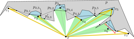
Figure 9: The crevices of obstacle $p$ (with respect to vertex $x$ in $X$) are the light blue regions that contain vertices $v_{2}$, $v_{3}$, and $v_{4}$ of $K$. Each extended crevice consists of a light blue and an adjacent light green region. The dotted line segments are the doors of the corresponding vertices. The red line segment pierces the crevice $Z_{6}$. The orange L-shapes assume $v_{1}\prec v_{2}\prec v_{3}\succ v_{4}\succ v_{5}\prec v_{6}\succ v_{7}$. With $\partial p$, two consecutive L-shapes enclose parts of at most three extended crevices.

• The crevice of $v_{i}$ is a polygon $Z_{i}$ whose boundary starts with the line segment $\overline{v_{i}p_{i,i+1}}$, then follows $\partial p$ in the clockwise direction, passes the point $p_{i}$, reaches the point $p_{i,i-1}$, and returns to $v_{i}$ along the line segment $\overline{p_{i,i-1}v_{i}}$.

• The extended crevice of $v_{i}$ is a polygon $Z_{i}^{\prime}$ whose boundary starts with the line segment $\overline{xp^{\prime}_{i,i+1}}$, then follows $\partial p$ in the clockwise direction, passes $p_{i}$, reaches $p^{\prime}_{i,i-1}$, and returns to $x$ along the line segment $\overline{p^{\prime}_{i,i-1}x}$.

We consider (extended) crevices as open; hence they do not intersect the polygon $p$ to which they belong. We use the term “crevice” here since, for every $i\in[g]$, the vertex $v_{i}$ sits in an indentation of $p$; see Figure 9. Note that there are $g-2$ extended crevices and that each of them contains precisely one crevice. No two extended crevices intersect, and the (extended) crevices are naturally ordered according to the numbering of the vertices from the perspective of $x$ as described above.

The reason why we define these (extended) crevices is that they will allow us to slightly alter $S$ to accommodate the before-mentioned additional vertex of $T$. To do so, we need to carefully avoid other obstacles as well as visibility edges. In the remainder of this part of the proof, we identify three types of “bad” (extended) crevices and show that each of these occurs only a bounded number of times.

First, we simply observe that at most $k-1$ extended crevices can contain a vertex of the vertex cover $X$ (because $|X\setminus\{x\}|=k-1$).

Second, we argue that every obstacle intersects only very few extended crevices (of $p$ with respect to $x$). To this end, observe that for every $i\in[g]$, the line segment $\overline{xv_{i}}$ is an edge of $G$ and as such it must not intersect any obstacle. Moreover, for every $i\in[g-1]$ with $v_{i}\prec v_{i+1}$, by the definition of $K$, no obstacle intersects the (open) line segment $\overline{v_{i}p_{i,i+1}}$. This line segment, together with $\overline{xv_{i}}$, forms an L-shape that does not intersect any obstacle (see, e.g., the orange L-shape at $v_{4}$ in Figure 9). Similarly, for every $1<i\leq g$ with $v_{i}\prec v_{i-1}$, the line segment $\overline{xv_{i}}$ and the open line segment $\overline{v_{i}p_{i,i-1}}$ form an L-shape that does not intersect any obstacle (see, e.g., the orange L-shape at $v_{2}$ in Figure 9). Together with $\partial p$, two consecutive L-shapes form a polygon whose boundary does not intersect any obstacles (other than $p$). The interior of such a polygon contains parts of at most one extended crevice (if $v_{i-1}\succ v_{i}\prec v_{i+1}$), parts of two extended crevices (if $v_{i-1}\prec v_{i}\prec v_{i+1}$ or $v_{i-1}\succ v_{i}\succ v_{i+1}$), or parts of three extended crevices (if $v_{i-1}\prec v_{i}\succ v_{i+1}$); see Figure 9. If $v_{1}\succ v_{2}$ and/or $v_{g-1}\prec v_{g}$, the parts of the extended crevices of $v_{2}$ and/or $v_{g-1}$ lie outside the region enclosed by $p$, the first L-shape, and the last L-shape. Hence any obstacle outside that region can intersect at most two extended crevices. Summarizing the above, we conclude that every obstacle can intersect at most three extended crevices. This implies that at most $3h\leq 3\cdot\big{(}\binom{k}{2}+k\cdot 2^{k}\big{)}$ extended crevices are intersected by obstacles.

Third, for $i\in[g]$, let the defining triangle of crevice $Z_{i}$ be the triangle $\triangle(v_{i},p_{i,i+1},p_{i,i-1})$, where $v_{i}$ is the tip of that triangle and the line segment $\overline{p_{i,i+1}p_{i,i-1}}$ is its door. (In Figure 9), the doors are dotted.) Note that the line segment $\overline{xv_{i}}$ may or may not cross the door of $v_{i}$. If $\overline{xv_{i}}$ does not cross the door (as in the case of $v_{2}$ and of $v_{4}$ in Figure 9), there could exist an edge $e$ of $G$ that crosses both non-door line segments of the defining triangle. In this case, we say that the crevice $Z_{i}$ is pierced (by the edge $e$). For example, the red solid line segment in Figure 9 pierces $Z_{4}$.

Claim 4.

Every sequence of at least $2k-1$ crevices contains at least one crevice that is not pierced.

Proof of the claim..

Assume, for a contraction, that there exists an index $j$ with $1<j<g-2k+2$ such that each of the $2k-1$ crevices in the sequence $Z_{j},Z_{j+1},\dots,Z_{j+2k-2}$ is pierced. This implies that, for $j\leq i\leq j+2k-2$, when going from $v_{i-1}$ to $v_{i+1}$, there is a left turn in $v_{i}$; see Figure 10. Hence the set $\{v_{j-1},v_{j},\dots,v_{j+2k-2},v_{j+2k-1}\}$ is the vertex set of a convex polygon (dashed in Figure 10) that contains the doors of $v_{j},\dots,v_{j+2k-2}$. Clearly, $x$ lies outside this convex polygon.

Consider an arbitrary vertex $u$ in the vertex cover $X$ of $G$. We show that at most two edges incident to $u$ pierce a crevice in our sequence. There are two ways how an edge $uv$ can pierce a crevice $Z_{i}$ in that sequence. When rotating $uv$ counterclockwise around $u$, $uv$ can either first hit the tip $v_{i}$ or first hit the door of $v_{i}$. In the former case, we say that $uv$ tip-pierces $Z_{i}$; in the latter case, $uv$ door-pierces $Z_{i}$. We show that $u$ can have at most one edge of either type. The arguments are symmetric, so it suffices to show that $u$ is incident to at most one edge that tip-pierces a crevice in our sequence. To this end, we define, for each index $i$ with $j\leq i\leq j+2k-2$, an open wedge $W_{i}$ with apex $v_{i}$ that is bounded by the ray $\overrightarrow{v_{i}v_{i+1}}$ and by the ray that starts in $v_{i}$ and is opposite to the ray $\overrightarrow{v_{i}v_{i-1}}$; see Figure 10. Note that, for different indices $i$ and $i^{\prime}$, wedges $W_{i}$ and $W_{i^{\prime}}$ are disjoint.

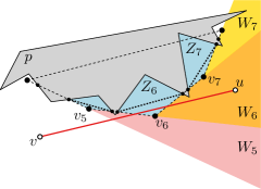
Figure 10: Wedges $W_{5}$, $W_{6}$, $W_{7}$ for crevices $Z_{5}$, $Z_{6}$, and $Z_{7}$. In order for an edge $uv$ to tip-pierce $Z_{6}$, $u$ must lie in wedge $W_{6}$.

We claim that, for an edge $uv$ to tip-pierce the crevice $Z_{i}$, vertex $u$ has to lie in wedge $W_{i}$. This is due to the fact that the ray $\overline{uv}$ must enter the defining triangle of $v_{i}$ via the edge $\overline{v_{i}v_{i,i+1}}$ and leave the defining triangle via the edge $\overline{v_{i}v_{i,i-1}}$. If $u$ does not lie in $W_{i}$ but in some $W_{i^{\prime}}$ with $i^{\prime}>i$, then $u$ does not see $v_{i}$ nor the edge $\overline{v_{i}v_{i,i+1}}$. If $u$ lies in some $W_{i^{\prime}}$ with $i^{\prime}<i$, then $u$ does not see the edge $\overline{v_{i}v_{i,i-1}}$ through the edge $\overline{v_{i}v_{i,i+1}}$.

Given our claim and the fact that the wedges are pairwise disjoint yields that $u$ is incident to at most one edge that tip-pierces a crevice (and, similarly, at most one edge that door-pierces a cervice. Hence, any vertex in $X\setminus\{x\}$ is incident to at most two edges that pierce crevices. Since $x$ sees $v_{1},\dots,v_{g}$, no edge incident to $x$ pierces a crevice. Hence, at most $2k-2$ of the crevices in the sequence $Z_{j},Z_{j+1},\dots,Z_{j+2k-2}$ can be pierced, which yields the desired contradiction.

∎

Claim 4 implies that every subsequence $(v_{j},v_{j+1},\dots,v_{j+2k})$ of consecutive vertices in $K$ must contain at least one crevice that is not pierced. Let an extended crevice $Z_{i}^{\prime}$ be good if $Z_{i}^{\prime}$ is not intersected by any obstacle, $Z_{i}^{\prime}\cap X=\emptyset$, and $Z_{i}$ is not pierced. Recall that $\texttt{cliquesize}(k)=15k\cdot 2^{k}$. In view of the bounds established above, we conclude that there must exist a sequence of good extended crevices of length at least

$$\texttt{crevicenum}(k) =\left(\left(\frac{\texttt{cliquesize}(k)-2}{2}-2\right)-\left((k-1)+3\cdot\binom{k}{2}+3\cdot k2^{k}\right)\right)\cdot\frac{1}{2k}$$

$$\geq\frac{(7.5\cdot k2^{k}-3)-(1.5\cdot k2^{k}+3\cdot k2^{k})}{2k}\qquad\text{using $k\leq 2^{k}$ }$$

$$\geq\frac{6.5\cdot k2^{k}-4.5\cdot k2^{k}}{2k}\geq 2^{k}\qquad\text{using $k2^{k}\geq 3$ for $k\geq 2$}$$

Extending $p$ in a Non-Obstructive Way.  From now on, we focus on good extended crevices in the aforementioned, sufficiently long sequence $Z^{\prime}_{\sigma(1)},Z^{\prime}_{\sigma(2)},\dots,Z^{\prime}_{\sigma(\texttt{crevicenum}(k))}$, where the $\sigma(i)$-th extended crevice $Z_{\sigma(i)}$ is defined by the vertex $v_{\sigma(i)}$ and the points $p_{\sigma(i),\sigma(i)+1}$, $p_{\sigma(i),\sigma(i)-1}$. Our aim in this section is to show that there exists some solution $S^{\circ}$ (which will either be $S$, or a slight adaptation of $S$) for $(G,h)$ which contains a crevice $Z_{\sigma(i)}$ where we can extend $p$ so as to accommodate an additional vertex of type $T$ without intersecting visibility lines between any pair of vertices that are adjacent in $G$.

We say that a good crevice $Z^{\prime}_{\sigma(i)}$ is perfect if it furthermore contains no vertex other than $v_{\sigma(i)}$. Next we claim that if we can show that $(G,h)$ admits a solution with a perfect crevice, we are essentially done. Recall that the graph $G^{\prime\prime}$ has vertex set $V(G^{\prime\prime})=V(G)\cup\{v\}$, where $v$ is the additional vertex of type $T$.

Claim 5.

If $(G,h)$ admits a solution with a perfect crevice, then $(G^{\prime\prime},h)$ also admits a solution.

Proof of the claim..

Let $i\in[\texttt{crevicenum}(k)]$ be such that $Z^{\prime}_{\sigma(i)}$ is a perfect crevice in a solution of $(G,h)$. We modify the obstacle $p$ that is adjacent to $Z^{\prime}_{\sigma(i)}$, in order to accommodate the additional vertex $v$ of type $T$. We add to $p$ a “thick” line segment that is orthogonal to the door of $v_{\sigma(i)}$ and stops very close to $v_{\sigma(i)}$, slightly to its right, say; see Figure 11.

Figure 11: Adding a vertex of type $T$ to a perfect crevice $Z^{\prime}_{\sigma(i)}$

Then we place $v$ to the right of this extension of $p$ such that $v_{\sigma(i)}$ and $v$ do not see each other. By making the extension thin and short enough and by placing $v$ sufficiently close to $v_{\sigma(i)}$, we can ensure that $v$ sees the same vertices as $v_{\sigma(i)}$ (namely those adjacent to $v_{\sigma(i)}$ in $G$). Since the extended crevice contains no other vertices and does not intersect any obstacles, this extension could only block a line of sight between two vertices outside of $Z^{\prime}_{\sigma(i)}$, but this line would pierce $Z_{\sigma(i)}$, contradicting the fact that $Z^{\prime}_{\sigma(i)}$ is good. Hence, we have obtained a solution for $(G^{\prime\prime},h)$. ∎

As a consequence, if a solution already contains a perfect crevice, we can invoke the previous claim to complete the proof. Unfortunately, it may happen that none of the at least $2^{k}$ good crevices in a solution is perfect. We now deal with this case.

Claim 6.

If the instance $(G,h)$ admits a solution, then $(G,h)$ admits also a solution with a perfect crevice.

Proof of the claim..

Let $S$ be a solution of $(G,h)$. If $S$ does not contain a perfect crevice, then each of the at least $2^{k}$ good crevices in $S$ must contain some vertex that is not part of the vertex cover $X$. Let $\mathcal{Z}$ be the set of (non-extended) crevices that correspond to the good crevices in $S$. We start by arguing that each crevice $Z_{\sigma(i)}$ in $\mathcal{Z}$ contains only a single vertex of type $T$, specifically $v_{\sigma(i)}$. Indeed, assume for a contradiction that $Z_{\sigma(i)}$ contains not only $v_{\sigma(i)}$ but also another vertex $w$ of the same type as $v_{\sigma(i)}$. Since $Z_{\sigma(i)}$ corresponds to a good crevice, $Z_{\sigma(i)}$ does not intersect any obstacle, and hence the visibility between $v_{\sigma(i)}$ and $w$ must be blocked by $p$. Similarly, the first obstacle hit when traversing the line segment from $w$ to the vertex $v_{\sigma(i)+1}$ in the next crevice $Z_{\sigma(i)+1}$ in our sequence must again be $p$ since this occurs on the boundary of $Z_{\sigma(i)}$. As a consequence, we obtain that $w$ is itself contained in a good crevice for $S$, contradicting the choice of $\mathcal{Z}$.

Next, we mark all of the crevices in $\mathcal{Z}$ as unprocessed and then iterate the following procedure. We choose an unprocessed crevice $Z_{\sigma(i)}\in\mathcal{Z}$ and consider the vertex $u$ in $Z_{\sigma(i)}$ that is farthest from the door in the direction away from $x$ (i.e., “inside” the crevice). Let the $u$-door be a line segment defined as follows. The $u$-door is parallel to the door of $v_{\sigma(i)}$, contains $u$, and starts and ends at the first intersection with the boundary of $p$ (i.e., the $u$-door extends from $p$ in both directions until it hits the boundary of the crevice; see the dotted line segment through $u$ in Figure 12(a)). By the choice of $u$, the part of $Z_{\sigma(i)}$ that is separated from $x$ by the $u$-door (darker blue in Figure 12(a)) contains no vertex at all.

(a) $u$ lies in the crevice of $v_{\sigma(i)}$

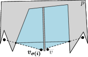
(b) accommodating all vertices of the same type as $u$

Figure 12: Reshaping the obstacle $p$ to establish the existence of a perfect extended crevice.

Hence, it is possible to extend the boundary of $p$ towards $u$ in this part of the crevice without intersecting any visibility lines of edges in $G$. Let $T_{u}$ be the set of all vertices of the same type as $u$ that occur in the crevices in $\mathcal{Z}$. We now extend $p$ by constructing a tiny haircomb-like structure in the immediate vicinity of $u$ with precisely $|T_{u}|$ slots; then we move each vertex in $T_{u}$ to a dedicated slot; see Figure 12(b). The teeth of the haircomb are long enough to block the visibilities between every pair of vertices in $T_{u}$, and they are short enough to preserve the visibilities between all other vertices in the graph (since the part of $Z_{\sigma(i)}$ behind the $u$-door is empty, and since all vertices are placed in the immediate vicinity of $u$).

At this point, we mark the crevice $Z_{\sigma(i)}$ and also the type $T_{u}$ as “processed”, and restart our considerations with the newly constructed solution and some unprocessed crevice. After $j$ steps of this procedure, we have processed precisely $j$ crevices, and none of the unprocessed crevices contains any vertex of a processed type. Since the number of types other than $T$ is upper-bounded by $2^{k}-1$, the procedure is guaranteed to construct a solution where at least one unprocessed crevice $Z_{\sigma(i^{\star})}$ contains only a single vertex $v_{\sigma(i^{\star})}$ of type $T$. By definition, $Z_{\sigma(i^{\star})}$ corresponds to a perfect crevice $Z^{\prime}_{\sigma(i^{\star})}$. ∎

In summary, we conclude that if $(G,h)$ is a YES-instance, then it must admit a solution $S$ with a perfect crevice. By Claim 5, this implies that $(G^{\prime\prime},h)$, where $G^{\prime\prime}$ is obtained by adding a vertex of type $T$ to $G$, is also a YES-instance. Moreover, we have already argued that if $(G^{\prime\prime},h)$ is a YES-instance, then so is $(G,h)$. Hence, if $G$ contains at least $\texttt{typesize}(k)$ vertices of type $T$, we can delete a vertex of type $T$ to obtain an equivalent instance. Iterating this step results in an equivalent instance $(H,h)$ where there are at most $\texttt{typesize}(k)$ vertices of each type. In particular, $H$ contains at most $k+(2^{k}\cdot\texttt{typesize}(k))$ many vertices. At this point, we can solve the instance by brute force in the manner described in Lemma 22. ∎

6 NP-Hardness of Deciding Whether a Given Obstacle is Enough

In this section, we investigate the complexity of the obstacle representation problem for the case that a single (outside) obstacle is given. In particular, we prove Theorem 8, which we restate here.

See 8

Proof.

We reduce from 3-Partition, which is NP-hard [10]. An instance of 3-Partition is a multiset $S$ of $3m$ positive integers $a_{1},\dots,a_{3m}$, and the question is whether $S$ can be partitioned into $m$ groups of cardinality 3 such that the numbers in each group sum up to the same value $B$, which is $(\sum_{i=1}^{3m}a_{i})/m$. The problem remains NP-hard if $B$ is polynomial in $m$ and if, for each $i\in[3m]$, it holds that $a_{i}\in(B/4,B/2)$.

Given a multiset $S$, we construct a graph $G$ and a simple polygon $P$ with the property that the vertices of $G$ can be placed in $P$ such that their visibility graph with respect to $P$ is isomorphic to $G$ if and only if $S$ is a yes-instance of 3-Partition.

Let $G$ be a clique with vertices $v_{1},\dots,v_{3m}$ where, for $i\in[3m]$, clique vertex $v_{i}$ is connected to $a_{i}$ leaves $\ell_{i,1},\dots,\ell_{i,a_{i}}$ (that is, vertices of degree 1). Note that $G$ has $3m+Bm$ vertices and $\binom{3m}{2}+Bm$ edges. The polygon $P$ (see Figure 13) is an orthogonal polygon with $m$ groups of $B$ bays (red in Figure 13) that are separated from each other by corridors (of height $B/4$ and width $4B$; light blue in Figures 13 and 14). Each bay is a unit square; any two consecutive bays are one unit apart. The height of $P$ (including the bays) is $B/2+1$. Hence, the sizes of $G$ and $P$ are polynomial in $m$.

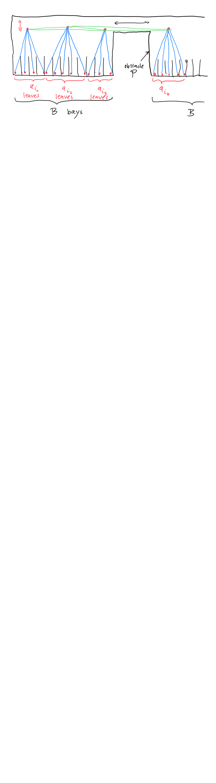
Figure 13: Idea of the reduction from 3-Partition

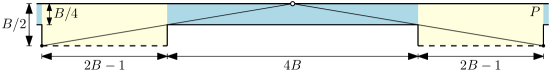
Figure 14: Size of the polygon $P$ used in our reduction; drawing not (quite) to scale

If $S$ is a yes-instance, then we can sort $S$ such that $\sum_{i=1}^{3}a_{i}=\dots=\sum_{i=3m-2}^{3m}a_{i}=B$. We place the leaves adjacent to $v_{1},\dots,v_{3m}$ into the $Bm$ bays of $P$, going through $P$ from left to right. We place each leaf at the center of its bay. Then, for $i\in[3m]$, we place vertex $v_{i}$ on the perpendicular bisector of its leftmost leaf $\ell_{i,1}$ and its rightmost leaf $\ell_{i,a_{i}}$ so that $v_{i}$ sees exactly the leaves $\ell_{i,1},\dots,\ell_{i,a_{i}}$ adjacent to $v_{i}$. This is achieved by setting the height of $v_{i}$ above its leaves to $a_{i}$ if $a_{i}$ is even and to $a_{i}-1$ otherwise. Recall that $B/4+1\leq a_{i}\leq B/2-1$. To make sure that even the lowest clique vertices can see each other through the corridors, we lift all clique vertices by half a unit. This does not change the set of bay centers that a clique vertex can see. (Note that Figure 13 does not reflect this slight modification.) The sizes of the corridors between consecutive groups of $B$ bays ensure that each clique vertex sees every other clique vertex but no clique vertex can see into bays of different groups; see Figure 14 (where the dashed line segments mark the top edges of the bays).

Given a yes-instance of the obstacle problem, that is, a placement of the vertices of $G$ in $P$ such that their visibility graph with respect to $P$ is isomorphic to $G$, we show how $S$ can be 3-partitioned. First, observe that no two leaves are adjacent in $G$; hence any convex region in $P$ contains at most one leaf. In particular, this holds for the yellow group regions in Figures 13 and 14, for each of the red bays, and for the bounding box of all blue corridors. Therefore, all but $m+1$ leaves lie in bays. By scaling the partition instance by a factor of $m+2$, we can assume that each leaf lies in a bay. Due to our above observation regarding the visibility region of clique vertices, we can map each clique vertex to a group of bays. Since we assumed that, for each $i\in[1,3m]$, $v_{i}\in(B/4,B/4)$, exactly three clique vertices are mapped to each group of bays. Since we can assume that every leaf lies in its own bay, the total number of leaves per group cannot exceed $B$. On the other hand, we must distribute a total of $mB$ leaves to $m$ groups, so each group must get exactly $B$ leaves. Hence the numbers of leaves of the three clique vertices in each group sums up to $B$, which 3-partitions $S$ as desired. ∎

References

- [1] Oswin Aichholzer, Jean Cardinal, Vincent Kusters, Stefan Langerman, and Pavel Valtr. Reconstructing point set order types from radial orderings. Int. J. Comput. Geom. Appl., 26(3-4):167–184, 2016. doi:10.1142/S0218195916600037.
- [2] Hannah Alpert, Christina Koch, and Joshua D. Laison. Obstacle numbers of graphs. Discrete Comput. Geom., 44(1):223–244, 2010. doi:10.1007/s00454-009-9233-8.
- [3] Martin Balko, Josef Cibulka, and Pavel Valtr. Drawing graphs using a small number of obstacles. Discrete Comput. Geom., 59(1):143–164, 2018. doi:10.1007/s00454-017-9919-2.
- [4] Jean Cardinal and Udo Hoffmann. Recognition and complexity of point visibility graphs. Discrete Comput. Geom., 57(1):164–178, 2017. doi:10.1007/s00454-016-9831-1.
- [5] Steven Chaplick, Fabian Lipp, Ji-won Park, and Alexander Wolff. Obstructing visibilities with one obstacle. In Yifan Hu and Martin Nöllenburg, editors, Proc. 24th Int. Symp. Graph Drawing & Network Vis. (GD), volume 9801 of LNCS, pages 295–308. Springer, 2016. URL: http://arxiv.org/abs/1607.00278, doi:10.1007/978-3-319-50106-2\_23.
- [6] Rodney G. Downey and Michael R. Fellows. Fundamentals of Parameterized Complexity. Texts in Computer Science. Springer, 2013. doi:10.1007/978-1-4471-5559-1.
- [7] Vida Dujmović and Pat Morin. On obstacle numbers. Electr. J. Comb., 22(3):#P3.1, 2015. doi:10.37236/4373.
- [8] Stefan Felsner and Pavel Valtr. Coding and counting arrangements of pseudolines. Discrete Comput. Geom., 46(3):405–416, 2011. doi:10.1007/s00454-011-9366-4.
- [9] Oksana Firman, Philipp Kindermann, Jonathan Klawitter, Boris Klemz, Felix Klesen, and Alexander Wolff. Outside-obstacle representations with all vertices on the outer face. In Patrizio Angelini and Reinhard von Hanxleden, editors, Proc. 30th Int. Symp. Graph Drawing & Network Vis. (GD), volume 13764 of LNCS, pages 432–440. Springer, 2023. doi:10.1007/978-3-031-22203-0_31.
- [10] Michael R. Garey and David S. Johnson. Complexity results for multiprocessor scheduling under resource constraints. SIAM J. Comput., 4(4):397–411, 1975. doi:10.1137/0204035.
- [11] Subir Kumar Ghosh and Bodhayan Roy. Some results on point visibility graphs. Theoret. Comput. Sci., 575:17–32, 2015. doi:10.1016/j.tcs.2014.10.042.
- [12] John Gimbel, Patrice Ossona de Mendez, and Pavel Valtr. Obstacle numbers of planar graphs. In Fabrizio Frati and Kwan-Liu Ma, editors, Proc. 25th Int. Symp. Graph Drawing & Netw. Vis. (GD), volume 10692 of LNCS, pages 67–80. Springer, 2018. doi:10.1007/978-3-319-73915-1_6.
- [13] Jacob E. Goodman and Richard Pollack. Upper bounds for configurations and polytopes in . Discrete Comput. Geom., 1(3):219–227, 1986. doi:10.1007/BF02187696.
- [14] Jacob E. Goodman and Richard Pollack. Allowable sequences and order types in Discrete and Computational Geometry. In New Trends in Discrete and Computational Geometry, volume 10 of Algorithms and Combinatorics, pages 103–134. Springer, Berlin, 1993. doi:10.1007/978-3-642-58043-7_6.
- [15] Matthew P. Johnson and Deniz Sarıöz. Representing a planar straight-line graph using few obstacles. In Proc. 26th Canadian Conf. Comput. Geom. (CCCG), pages 95–99, 2014. URL: http://www.cccg.ca/proceedings/2014/papers/paper14.pdf.
- [16] Donald E. Knuth. Axioms and Hulls, volume 606 of LNCS. Springer, Heidelberg, Germany, 1992. doi:10.1007/3-540-55611-7.
- [17] Padmini Mukkamala, János Pach, and Dömötör Pálvölgyi. Lower bounds on the obstacle number of graphs. Electr. J. Comb., 19(2):#P32, 2012. doi:10.37236/2380.
- [18] Frank P. Ramsey. On a problem of formal logic. Proc. London Math. Soc. (2), 30(4):264–286, 1929. doi:10.1112/plms/s2-30.1.264.
- [19] James Renegar. On the computational complexity and geometry of the First-order Theory of the Reals, Part I: Introduction. Preliminaries. The geometry of semi-algebraic sets. The decision problem for the Existential Theory of the Reals. J. Symb. Comput., 13(3):255–300, 1992. doi:10.1016/S0747-7171(10)80003-3.
- [20] James Renegar. On the computational complexity and geometry of the first-order theory of the reals. Part II: The general decision problem. Preliminaries for quantifier elimination. J. Symb. Comput., 13(3):301–327, 1992. doi:10.1016/S0747-7171(10)80004-5.
- [21] James Renegar. On the computational complexity and geometry of the first-order theory of the reals. Part III: Quantifier elimination. J. Symb. Comput., 13(3):329–352, 1992. doi:10.1016/S0747-7171(10)80005-7.
- [22] Emo Welzl. Constructing the visibility graph for line segments in time. Inform. Process. Lett., 20:167–171, 1985. doi:10.1016/0020-0190(85)90044-4.