PolarFormer: Multi-camera 3D Object Detection with Polar Transformer

Abstract

3D object detection in autonomous driving aims to reason “what” and “where” the objects of interest present in a 3D world. Following the conventional wisdom of previous 2D object detection, existing methods often adopt the canonical Cartesian coordinate system with perpendicular axis. However, we conjugate that this does not fit the nature of the ego car’s perspective, as each onboard camera perceives the world in shape of wedge intrinsic to the imaging geometry with radical (non-perpendicular) axis. Hence, in this paper we advocate the exploitation of the Polar coordinate system and propose a new Polar Transformer (PolarFormer) for more accurate 3D object detection in the bird’s-eye-view (BEV) taking as input only multi-camera 2D images. Specifically, we design a cross-attention based Polar detection head without restriction to the shape of input structure to deal with irregular Polar grids. For tackling the unconstrained object scale variations along Polar’s distance dimension, we further introduce a multi-scale Polar representation learning strategy. As a result, our model can make best use of the Polar representation rasterized via attending to the corresponding image observation in a sequence-to-sequence fashion subject to the geometric constraints. Thorough experiments on the nuScenes dataset demonstrate that our PolarFormer outperforms significantly state-of-the-art 3D object detection alternatives.

Introduction

Figure 1: Taking multi-camera images as input, the proposed PolarFormer model is designed particularly for accurate 3D object detection in the Polar coordinate system.

3D object detection is an enabling capability of autonomous driving in unconstrained real-world scenes (Wang et al. 2022b, 2021). It aims to predict the location, dimension and orientation of individual objects of interest in a 3D world. Despite favourable cost advantages, multi-camera based 3D object detection (Wang et al. 2021, 2022a, 2022b; Zhou, Wang, and Krähenbühl 2019) remains particularly challenging. To obtain 3D representation, dense depth estimation is often leveraged (Philion and Fidler 2020), which however is not only expensive in computation but error prone. To bypass depth inference, more recent methods (Wang et al. 2022b; Li et al. 2022) exploit query-based 2D detection (Carion et al. 2020) to learn a set of sparse and virtual embedding for multi-camera 3D object detection, yet incapable of effectively modeling the geometry structure among objects. Typically, the canonical Cartesian coordinate system with perpendicular axis is adopted in either 2D (Zhou, Wang, and Krähenbühl 2019; Wang et al. 2021) or 3D (Wang et al. 2022b; Li et al. 2022) space. This is largely restricted by convolution based models used. In contrast, the physical world perceived under each camera in the ego car’s perspective is in shape of wedge intrinsic to the camera imaging geometry with radical non-perpendicular axis (Figure 5). Bearing this imaging property in mind, we conjugate that the Polar coordinate system should be more appropriate and natural than the often adopted Cartesian counterpart for 3D object detection. Indeed, the Polar coordinate has been exploited in a few LiDAR-based 3D perception methods (Zhang et al. 2020; Bewley et al. 2020; Rapoport-Lavie and Raviv 2021; Zhu et al. 2021b). However, they are limited algorithmically due to the adoption of convolutional networks restricted to rectangular grid structure and local receptive fields.

Motivated by the aforementioned insights, in this work a novel Polar Transformer (PolarFormer) model for multi-camera 3D object detection in a Polar coordinate system is introduced (Figure 4). Specifically, we first learn the representation of polar rays corresponding to image regions in a sequence-to-sequence cross-attention formulation. Then we rasterize a BEV Polar representation consisting of a set of Polar rays evenly distributed around 360 degrees. To deal with irregular Polar grids as suffered by conventional LiDAR based solutions (Zhang et al. 2020; Bewley et al. 2020; Rapoport-Lavie and Raviv 2021; Zhu et al. 2021b), we propose a cross-attention based decoder head design without restriction to the shape of input structure. For tackling the challenge of unconstrained object scale variation along Polar’s distance dimension, we resort to a multi-scale Polar BEV representation learning strategy.

The contributions of this work are summarized as follows: (I) We propose a new Polar Transformer (PolarFormer) model for multi-camera 3D object detection in the Polar coordinate system. (II) This is achieved based on two Polar-tailored designs: A cross-attention based decoder design for dealing with the irregular Polar girds, and a multi-scale Polar representation learning strategy for handling the unconstrained object scale variations over Polar’s distance dimension. (III) Extensive experiments on the nuScenes dataset show that our PolarFormer achieves leading performance for camera-based 3D object detection (Figure 1).

Related work

Monocular/multi-camera 3D object detection

Image-based 3D object detection aims to estimate the object location, dimension and orientation in the 3D space alongside its category given only image input. To solve this ill-posed problem, (Zhou, Wang, and Krähenbühl 2019; Wang et al. 2021) naively build their detection pipelines by augmenting 2D detectors (Zhou, Wang, and Krähenbühl 2019; Tian et al. 2019) in a data driven fashion. PGD (Wang et al. 2022a) further captures the uncertainty and models the relationship of different objects by utilizing geometric prior. Contrast to the above image-only methods, depth-based methods (Xu and Chen 2018; Ding et al. 2020; Wang et al. 2019; You et al. 2019; Ma et al. 2019; Reading et al. 2021) use depth cues as 3D information to mitigate the naturally ill-posed problem. Recently, multi-camera-based 3D object detection emerges. DETR3D (Wang et al. 2022b) considers detecting objects across all cameras collectively. It learns a set of sparse and virtual query embedding, without explicitly building the geometry structure among objects/queries.  (Li et al. 2022) considers detecting objects in BEV, performing end-to-end object detection via object queries. Note that multi-camera setting uses the same amount of training data as the monocular pipelines. Both multi-camera and monocular paradigms share the same evaluation metrics.

Bird’s-eye-view (BEV) representation

Recently there is a surge of interest in transforming the monocular or multi-view images from ego car cameras into the bird’s-eye-view coordinate (Roddick, Kendall, and Cipolla 2019; Philion and Fidler 2020; Li et al. 2021; Roddick and Cipolla 2020; Reading et al. 2021; Saha et al. 2022) followed by specific optimization tasks (e.g., 3D object detection, semantic segmentation). A natural solution (Philion and Fidler 2020; Hu et al. 2021) is to learn the BEV representation by leveraging the pixel-level dense depth estimation. This however is error-prone due to lacking ground-truth supervision. Another line of research aims to bypass the depth prediction and directly leverage a Transformer (Chitta, Prakash, and Geiger 2021; Can et al. 2021; Saha et al. 2022) or a FC layer (Li et al. 2021; Roddick and Cipolla 2020; Yang et al. 2021) to learn the transformation from camera inputs to the BEV coordinate. A similar attempt as ours is conducted in (Saha et al. 2022) but limited in a couple of aspects: (i) It is restricted to monocular input for a straightforward 2D segmentation task while we consider multiple cameras collectively for more challenging 3D object detection; (ii) We uniquely provide a solid multi-scale Polar BEV transformation to tackle the unconstrained object scale variations and followed by a jointly optimized cross-attention based Polar head.

3D object detection in Polar coordinate

3D object detection in the Polar or Polar-like coordinate system has been attempted in LiDAR-based perception methods. For example, CyliNet (Zhu et al. 2021b) introduces range-based guidance for extracting Polar-consistent features. In particular, it adapts a Cartesian heatmap to a Polar version for object classification, whilst learning relative heading angles and velocities. However, CyliNet still lags clearly behind the Cartesian counterpart. Recently, PolarSteam (Chen, Vora, and Beijbom 2021) designs a learnable sampling module for relieving object distortion in Polar coordinate and uses range-stratified convolution and normalization for flexibly extracting the features over different ranges. Limited by the convolution based network, it remains inferior despite of these special designs. In contrast to all these works, we resort to the cross-attention mechanism, tackling the challenges of object scale variance and appearance distortion in the Polar coordinate principally.

Method

\begin{overpic}[width=516.00995pt]{images/pipeline.pdf} \put(43.0,31.0){{(a)}} \put(40.0,29.5){Cross-plane} \put(41.0,28.0){encoder} \put(27.0,48.0){{(b)} Polar alignment module} \put(62.0,13.5){{(c)}} \put(59.5,12.0){Polar BEV} \put(61.0,10.5){encoder} \end{overpic}

Figure 2: Schematic illustration of our proposed PolarFormer for multi-camera 3D object detection. For each image captured by any camera view, our model first extracts the feature maps at multiple spatial scales. Given such a feature map, the cross-plane encoder (a) then transforms all the feature columns to a set of Polar rays in a sequence-to-sequence manner via polar queries based cross-attention. The polar rays from all the cameras are subsequently processed by a Polar alignment module (b) to generate a structured multi-scale Polar BEV map, followed by further enhancement via interactions among different scales using a Polar BEV encoder (c). At last, a specially designed Polar Head decodes multi-scale Polar BEV features for making final predictions in the Polar coordinate.

In 3D object detection task, we are given a set of $N$ monocular views $\{\mathbf{I_{n}},\mathbf{\Pi_{n}},\mathbf{E_{n}}\}_{n=1}^{N}$ consisting of input images $\mathbf{I_{n}}\in\mathbb{R}^{H\times W\times 3}$, camera intrinsics $\mathbf{\Pi_{n}}\in\mathbb{R}^{3\times 3}$ and camera extrinsics $\mathbf{E_{n}}\in\mathbb{R}^{4\times 4}$. The objective of our Polar Transformer (PolarFormer) is to learn an effective BEV Polar representation from multiple camera views for facilitating the prediction of object locations, dimensions, orientations and velocities in the Polar coordinate system. PolarFormer consists of the following components. A cross-plane encoder first produces a multi-scale feature representation of each input image, characterized by a cross-plane attention mechanism in which Polar queries attend to input images to generate 3D features in BEV. A Polar alignment module then aggregates Polar rays from multiple camera views to generate a structured Polar map. Further, a BEV Polar encoder enhances the Polar features with multi-scale feature interaction. Finally, a Polar detection head decodes the Polar map and predicts the objects in the Polar coordinate system. For tackling the unconstrained object scale variation with multi-granularity of details, we consider a multi-scale BEV Polar representation structure. As shown in Figure 4, image features with different scales have unique cross-plane encoders and interact with each other in a shared Polar BEV encoder. Multi-scale Polar BEV maps are then queried by Polar decoder head. An overall architecture of PolarFormer is depicted in Figure 2.

Cross-plane encoder

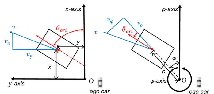
Figure 3: Cartesian and Polar coordinates.

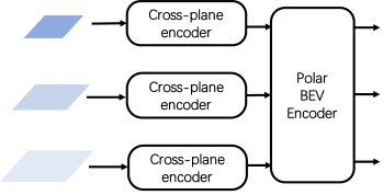
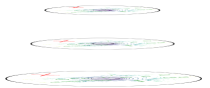
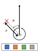
Figure 4: Multi-scale Polar BEV maps.

The goal of cross-plane encoder is to associate an image with BEV Polar rays. According to the geometric model of camera, for any camera coordinate $(x^{(C)},y^{(C)},z^{(C)})\in\mathbb{R}^{3}$, the transformation to image coordinate $(x^{(I)},y^{(I)})\in\mathbb{R}^{2}$could be described as:

$$s\begin{bmatrix}x^{(I)}\\ y^{(I)}\\ 1\end{bmatrix}=\begin{bmatrix}f_{x}&0&u_{0}\\ 0&f_{y}&v_{0}\\ 0&0&1\end{bmatrix}\begin{bmatrix}x^{(C)}\\ y^{(C)}\\ z^{(C)}\end{bmatrix},$$ (1)

where $f_{x}$, $f_{y}$, $u_{0}$ and $v_{0}$ are camera intrinsic parameters in $\mathbf{\Pi}$, $x^{(C)}$, $y^{(C)}$ and $z^{(C)}$ are the horizontal, vertical, depth coordinate respectively. $s$ is the scale factor. For any BEV Polar coordinate $(\rho^{(P)},\phi^{(P)})$, we have:

$$\phi^{(P)}=\arctan\frac{x^{(C)}}{z^{(C)}}=\arctan\frac{x^{(I)}-u_{0}}{f_{x}},$$ (2)

$$\begin{split}\rho^{(P)}=\sqrt{(x^{(C)})^{2}+(z^{(C)})^{2}}=z^{(C)}\sqrt{(\frac{x^{(I)}-u_{0}}{f_{x}})^{2}+1}.\end{split}$$ (3)

Eq. (2) suggests that the azimuth $\phi^{(P)}$ is irrelevant to the vertical value of image coordinate. It is hence natural to build a one-to-one relationship between Polar rays and image columns (Saha et al. 2022). However, we need object depth $z^{(C)}$ to compute radius $\rho^{(P)}$, the estimation of which is ill-posed. Instead of explicit depth estimation, we leverage the attention mechanism (Vaswani et al. 2017) to model the relationship between pixels along the image column and positions along the Polar ray.

Let $\mathbf{f}_{n,u,w}\in\mathbb{R}^{H_{u}\times C}$ represent the image column from $n$th camera, $u$th scale and $w$th column, and $\mathbf{\dot{p}}_{n,u,w}\in\mathbb{R}^{R_{u}\times C}$ denote the corresponding Polar ray query we introduce, where $H$ and $R$ are the image feature map’s height and Polar map’s range. We formulate cross-plane attention as:

$$\begin{split}\mathbf{p}_{n,u,w}&=\mathrm{MultiHead}(\mathbf{\dot{p}}_{n,u,w},\mathbf{f}_{n,u,w},\mathbf{f}_{n,u,w})\\ &=\mathrm{Concat}(\mathrm{head_{1}},\dots,\mathrm{head_{h}})\mathbf{W}^{O}_{u},\end{split}$$ (4)

where

$$\begin{split}\mathrm{head_{i}}\!=\!\mathrm{Attention}(\mathbf{\dot{p}}_{n,u,w}\mathbf{W}_{i,u}^{Q},\mathbf{f}_{n,u,w}\mathbf{W}_{i,u}^{K},\mathbf{f}_{n,u,w}\mathbf{W}_{i,u}^{V}),\end{split}$$ (5)

where $\mathbf{W}_{i,u}^{Q}\in\mathbb{R}^{d_{model}\times d_{q}}$, $\mathbf{W}_{i,u}^{K}\in\mathbb{R}^{d_{model}\times d_{k}}$, $\mathbf{W}_{i,u}^{V}\in\mathbb{R}^{d_{model}\times d_{v}}$, $\mathbf{W}^{O}_{u}\in\mathbb{R}^{hd_{model}\times d_{k}}$ are the projection parameters, $d_{q}=d_{k}=d_{v}=d_{model}/h$, $d$ is the feature dimension and $h$ is the number of heads.

Stacking the Polar ray features $\mathbf{p}_{n,u,w}\in\mathbb{R}^{R_{u}\times C}$ along azimuth axis, we obtain the Polar feature map (i.e., BEV Polar representation) $\mathbf{P}_{n,u}$ for $n$th camera and $u$th scale as:

$$\mathbf{P}_{n,u}\!=\!\mathrm{Stack}([\mathbf{p}_{n,u,1},\dots,\mathbf{p}_{n,u,W_{u}}],\mathrm{dim}\!=\!1)\!\in\!\mathbb{R}^{R_{u}\!\times\!W_{u}\!\times\!C},$$ (6)

where $W_{u}$ denotes the azimuth dimension. This sequence-to-sequence cross-attention-based encoder can encode geometric imaging prior and implicitly learn a proxy for depth efficiently. Next, we show how to integrate independent Polar rays from multiple cameras into a coherent and structured Polar BEV map.

Polar alignment across multiple cameras

Our Polar alignment module transforms Polar rays from different camera coordinates to a shared world coordinate. Taking multi-view Polar feature maps $\{\mathbf{P}_{n,u}\}_{n=1}^{N}$ and camera matrix $\{\mathbf{\Pi}_{n},\mathbf{E}_{n}\}_{n=1}^{N}$as inputs, it produces a coherent BEV Polar map $\mathbf{G}_{u}\in\mathbb{R}^{\mathcal{R}_{u}\times\mathcal{N}_{u}\times\mathcal{C}}$, covering all camera views, where $\mathcal{R}_{u}$, $\mathcal{N}_{u}$ and $\mathcal{C}$ are the dimensions of radius, azimuth and feature. Concretely, it first generates a set of 3D points in the cylindrical coordinate uniformly, denoted by $\mathcal{G}^{(P)}=\{(\rho^{(P)}_{i},\phi^{(P)}_{j},z^{(P)}_{k})|i=1,\dots,\mathcal{R}_{u};j=1,\dots,\mathcal{N}_{u};k=1,\dots,\mathcal{Z}_{u}\}$, where $\mathcal{Z}_{u}$ is the number of points along $z$ axis. Since cylindrical coordinate and Polar coordinate share radius and azimuth axis, their superscripts are both denoted with $P$. The points are then projected to the image plane of $n$th camera to retrieve the index of Polar ray, estimated by:

$$\begin{bmatrix}sx^{(I)}_{i,j,k,n}\\[5.0pt] sy^{(I)}_{i,j,k,n}\\[5.0pt] s\\[5.0pt] 1\end{bmatrix}=\begin{bmatrix}\mathbf{\Pi}_{n}&0\\ 0&1\end{bmatrix}\mathbf{E}_{n}\begin{bmatrix}\rho^{(P)}_{i}\sin{\phi^{(P)}_{j}}\\[5.0pt] \rho^{(P)}_{i}\cos{\phi^{(P)}_{j}}\\[5.0pt] z^{(P)}_{k}\\[5.0pt] 1\end{bmatrix},$$ (7)

where $s$ is the scale factor. Coherent BEV Polar map of $u$th scale can be then generated by:

$$\begin{split}&\mathbf{G}_{u}(\rho^{(P)}_{i},\phi^{(P)}_{j})=\frac{1}{\sum_{n=1}^{N}\sum_{k=1}^{\mathcal{Z}}\lambda_{n}(\rho^{(P)}_{i},\phi^{(P)}_{j},z^{(P)}_{k})}\\ &\cdot\sum_{n=1}^{N}\sum_{k=1}^{\mathcal{Z}}\lambda_{n}(\rho^{(P)}_{i},\phi^{(P)}_{j},z^{(P)}_{k}){\mathcal{B}(\mathbf{P}_{n,u},(\overline{x}^{(I)}_{i,j,k,n},\overline{r}_{i,j,n}))},\end{split}$$ (8)

where $\lambda_{n}(\rho^{(P)}_{i},\phi^{(P)}_{j},z^{(P)}_{k})$ is binary weighted factor indicating visibility in $n$th camera, $\mathcal{B}(\mathbf{P},(x,y))$ denotes the bilinear sampling $\mathbf{P}$ at location $(x,y)$, $\overline{x}^{(I)}_{i,j,k,n}$ and $\overline{r}_{i,j,n}$ denote the normalized Polar ray index and radius index. Note the radius $r$ is the distance between the point and the camera origin in BEV. Our Polar alignment module incorporates the features at different heights by generating the points along $z$ axis. As validated in Table 5(c), learning Polar representation is superior over Cartesian coordinate due to minimal information loss and higher consistency with raw visual data.

Table 1: State-of-the-art comparison on nuScenes test set. ${\dagger}$ denotes the prototype setting: The model is initialized from a FCOS3D (Wang et al. 2021) checkpoint trained on the nuScenes 3D detection dataset. ${\ddagger}$ denotes the improved setting: A pretrained model from DD3D (Park et al. 2021) is used, which includes external data from DDAD (Guizilini et al. 2020). $*$ denotes backbone is pretrained on COCO (Lin et al. 2014) and nuImage (Caesar et al. 2020).

Methods		Backbone	mAP$\uparrow$	NDS$\uparrow$		mATE$\downarrow$	mASE$\downarrow$	mAOE$\downarrow$	mAVE$\downarrow$	mAAE$\downarrow$
FCOS3D† (Wang et al. 2021)		R101	35.8	42.8		69.0	24.9	45.2	143.4	12.4
PGD† (Wang et al. 2022a)		R101	38.6	44.8		62.6	24.5	45.1	150.9	12.7
Ego3RT† (Lu et al. 2022)		R101	38.9	44.3		59.9	26.8	47.0	116.9	17.2
BEVFormer-S† (Li et al. 2022)		R101	40.9	46.2		65.0	26.1	43.9	92.5	14.7
PolarFormer†		R101	41.5	47.0		65.7	26.3	40.5	91.1	13.9
BEVFormer† (Li et al. 2022)		R101	44.5	53.5		63.1	25.7	40.5	43.5	14.3
PolarFormer-T†		R101	45.7	54.3		61.2	25.7	39.2	46.7	12.9
DETR3D‡ (Wang et al. 2022b)		V2-99	41.2	47.9		64.1	25.5	39.4	84.5	13.3
M2BEV∗ (Xie et al. 2022)		X101	42.9	47.4		58.3	25.4	37.6	10.53	19.0
Ego3RT‡ (Lu et al. 2022)		V2-99	42.5	47.9		54.9	26.4	43.3	101.4	14.5
BEVFormer-S‡		V2-99	43.5	49.5		58.9	25.4	40.2	84.2	13.1
PolarFormer‡		V2-99	45.5	50.3		59.2	25.8	38.9	87.0	13.2
BEVFormer‡ (Li et al. 2022)		V2-99	48.1	56.9		58.2	25.6	37.5	37.8	12.6
PolarFormer-T‡		V2-99	49.3	57.2		55.6	25.6	36.4	44.0	12.7

Polar BEV encoder at multiple scales

We leverage multi-scale feature maps for handling object scale variance in the Polar coordinate. To that end, the BEV Polar encoder performs information exchange among neighbouring pixels and across multi-scale feature maps. Formally, let $\{\mathbf{G}_{u}\}_{u=1}^{U}$ be the input multi-scale Polar feature maps and $\hat{x}_{q}\in[0,1]^{2}$ be the normalized coordinates of the reference points for each qeury element $q$, we introduce a multi-scale deformable attention module (Zhu et al. 2021a) as:

$$\begin{split}&\mathrm{MSDeformAttn}(\mathbf{z}_{q},x_{q},\{\mathbf{G}_{u}\}_{u=1}^{U})=\\ &\sum_{m=1}^{M}\mathbf{W}_{m}[\sum_{u=1}^{U}\sum_{k=1}^{K}A_{muqk}\mathbf{W^{\prime}}_{m}\mathbf{G}_{u}(\zeta_{u}(\hat{x}_{q})+\Delta x_{muqk})],\end{split}$$ (9)

where $m$ and $k$ are the index of the attention head and the sampling point. $\mathbf{z}_{q}$ is the query feature. $\Delta x_{muqk}$ and $A_{muqk}$ denote the sampling offset and the attention weight of the $k$th sampling point in $u$th feature level and $m$th attention head. The attention weight $A_{muqk}$ is normalized by $\sum_{u=1}^{U}\sum_{k=1}^{K}A_{muqk}=1$. Sampling offsets $\Delta x_{muqk}$ are generated by applying MLP layers on query $q$. Function $\zeta_{u}$ generates the sampling offsets and rescales the normalized coordinate $\hat{x}_{q}$ to the $u$th feature scale. $\mathbf{W}_{m}$ and $\mathbf{W}^{\prime}_{m}$ are learnable parameters. Serving as query, each pixel in the multi-scale feature maps exploits the information from both neighbouring pixels and pixels across scales. This enables learning richer semantics across all feature scales.

Polar BEV decoder at multiple scales

The Polar decoder decodes the above multi-scale Polar features to make predictions in the Polar coordinate. We construct the Polar BEV decoder with deformable attention (Zhu et al. 2021a). Specifically, we query $q$ in Eq. (9) as learnable parameters.

Unlike 2D reference points in the encoder, here the reference points are in 3D cylindrical coordinate, equal to Polar coordinate when projected to BEV. The classification branch in each decoder layer outputs the confidence score vector $\mathbf{c}\in\mathbb{R}^{\mathcal{O}}$, where $\mathcal{O}$ is the number of categories. The key learning targets of regression branch are in polar coordinate instead of Cartesian coordiante, as illustrated in Figure 4. For simplicity, superscript ^(P) is omitted. Reference points $(\rho,\phi,z)$ are iteratively refined in the decoder. With reference points, the regression branch regresses the offsets $d_{\rho}$, $d_{\phi}$ and $d_{z}$. The learning targets for orientation $\theta$ and velocity $v$ are relative to azimuths of objects and separated to orthogonal components $\theta_{\phi}$, $\theta_{\rho}$, $v_{\phi}$ and $v_{\rho}$, defined by:

$$\bar{\theta}_{ori}=\theta_{ori}-\phi,\quad\ \theta_{\phi}=\sin{\bar{\theta}_{ori}},\quad\ \theta_{\rho}=\cos{\bar{\theta}_{ori}},$$ (10)

and

$$\bar{\theta}_{v}=\theta_{v}-\phi,\quad\ v_{\phi}=v_{abs}\sin{\bar{\theta}_{v}},\quad\ v_{\rho}=v_{abs}\cos{\bar{\theta}_{v}}.$$ (11)

Here, $\theta_{ori}$ is the yaw angle of the bounding box. $v_{abs}$ and $\theta_{v}$ are the absolute value and angle of velocity. We regress the object size $l$, $w$ and $h$ as $\log l$, $\log w$ and $\log h$. We adopt Focal loss (Lin et al. 2017) and L1 loss for classification and regression respectively.

Experiments

Table 2: 3D object detection results in different coordinate systems and ablations for the model architecture. PC denotes feature in Polar and prediction in Cartesian.

Method	Feature	Prediction	mAP$\uparrow$	NDS$\uparrow$
Centerpoint (Yin, Zhou, and Krähenbühl 2021)	Cartesian	Cartesian	37.8	45.4
Centerpoint* (Yin, Zhou, and Krähenbühl 2021)	Cartesian	Cartesian	38.5	45.6
PolarFormer-CC	Cartesian	Cartesian	38.1	45.5
PolarFormer-PC	Polar	Cartesian	38.5	45.0
PolarFormer	Polar	Polar	39.6	45.8

(a) Ablation study on coordinate system and detection head.

Position encoding	mAP$\uparrow$	NDS$\uparrow$
2D learnable PE	38.8	45.1
3D PE	38.5	44.9
Fixed Sine PE	39.6	45.8

(b) Ablation on positional encoding (PE).

Methods	Multi-scale	mAP$\uparrow$	NDS$\uparrow$	mAOE$\downarrow$
PolarFormer-CC-s	✗	38.1	44.9	40.0
PolarFormer-PC-s	✗	38.8	45.0	37.6
PolarFormer-s	✗	39.1	45.0	37.3
PolarFormer-CC	✓	38.1	45.0	37.5
PolarFormer-PC	✓	38.5	45.5	40.8
PolarFormer	✓	39.6	45.8	37.5

(c) Effectiveness of multi-scale polar representation.

$\bm{\mathcal{N}_{1}}$	$\bm{\mathcal{R}_{1}}$		mAP$\uparrow$	NDS$\uparrow$
240	64		38.8	45.0
256	64		39.6	45.8
272	64		38.8	45.0
256	56		38.7	45.4
256	72		38.5	45.4
256	80		38.7	45.6

(d) Ablation on polar resolution.

Dataset

We evaluate the PolarFormer on the nuScenes dataset (Caesar et al. 2020). It provides images with a resolution of $1600\times 900$ from 6 surrounding cameras (Figure 1). The total of 1000 scenes, where each sequence is roughly 20 seconds long and annotated every 0.5 second, is split officially into train/val/test set with 700/150/150 scenes.

Implementation details

We implement our approach based on the codebase mmdetection3d (Contributors 2020). Following DETR3D (Wang et al. 2022b) and FCOS3D (Wang et al. 2021), a ResNet-101 (He et al. 2016), with 3rd and 4th stages equipped with deformable convolutions is adopted as the backbone architecture. The number of cross-plane encoder layer is set to 3 for each feature scale. The resolution of radius and azimuth for our multi-scale Polar BEV maps are (64, 256), (32, 128), (16, 64) respectively. We use 6 Polar BEV encoder and 6 decoder layers. Following DETR3D (Wang et al. 2022b), our backbone is initialized from a checkpoint of FCOS3D (Wang et al. 2021) trained on nuScenes 3D detection task, while the rest is initialized randomly. We use above setting for prototype verification. To fully leverage the sequence data, we further conduct temporal fusion between the current frame and one history sweep in the BEV space. Following BEVDet4D (Huang and Huang 2022), we simply concatenate two temporally adjacent multi-scale Polar BEV maps along the feature dimension and feed to the BEV Polar encoder. We randomly sample a history sweep from [3T; 27T] during training, and sample the frame at 15T for inference. T ($\approx 0.083s$) refers to the time interval between two sweep frames. We term our temporal version as PolarFormer-T.

Training

Following DETR3D (Wang et al. 2022b) we train our models for 24 epochs with the AdamW optimizer and cosine annealing learning rate scheduler on 8 NVIDIA V100 GPUs. The initial learning rate is $2\times 10^{-4}$, and the weight decay is set to $0.075$. Total batch size is set to 48 across six cameras. Synchronized batch normalization is adopted. All experiments use the original input resolution. Note our image variant uses the same amount of training data as the monocular pipelines (Wang et al. 2021) and the multi-camera counterparts (Wang et al. 2022b; Li et al. 2022). Multi-camera and monocular paradigms share the same evaluation metrics.

Inference

We evaluate our model on nuScenes validation set and test server. We do not adopt model-agnostic trick such as model ensemble and test time augmentation.

Comparison with the state of the art

We compare our method with the state of the art on both test and val sets of nuScenes. In addition to the (i) prototype setting mentioned in implementation details, we also evaluate our model in the (ii) improved setting, with VoVNet (V2-99) (Lee et al. 2019) as backbone architecture with a pretrained checkpoint from DD3D (Park et al. 2021) (fine-tuned on extra DDAD15M (Guizilini et al. 2020) dataset) to boost performance.

Table 1 compares the results on nuScenes test set. We observe that our PolarFormer achieves the best performance under both the (i) prototype and (ii) improved setting in terms of mAP and NDS metrics, indicating the superiority of learning representation in the Polar coordinate. With temporal information PolarFormer-T can further boot performance substantially. Additional experiments results on val set t and qualitative results are shown in supplementary materials.

Ablation studies

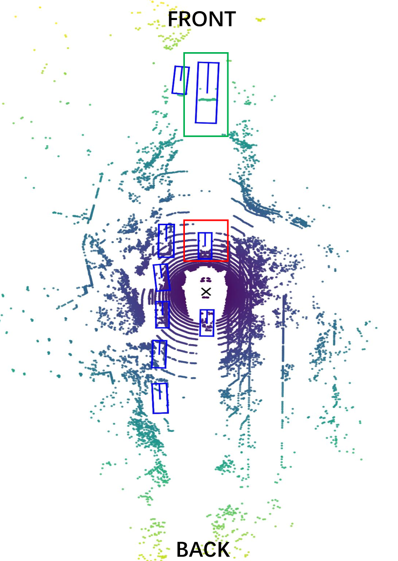
(a)

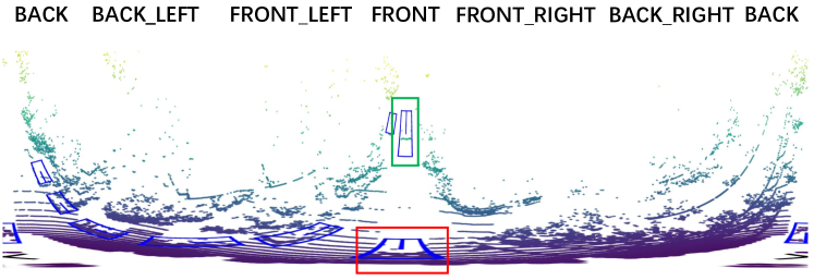
(b)

Method	Coordinate	Near	Medium	Far
DETR3D (Wang et al. 2022b)	Cartesian	49.9/49.3	28.6/39.2	8.1/21.2
BEVFormer-S (Li et al. 2022)	Cartesian	54.2/53.5	31.7/41.3	9.5/21.9
PolarFormer-CC	Cartesian	54.7/55.5	32.3/42.2	9.4/22.2
PolarFormer	Polar	57.8/55.8	33.6/42.9	9.6/22.3

(c)

Figure 5: 3D object detection in (a) Cartesian BEV vs. (b) Polar BEV, and (c) Performance comparison (mAP/NDS) at three distances (Near/Medium/Far). Red and green boxes show the same objects in different coordinates.

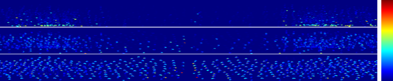
Figure 6: Multi-scale Polar BEV attention.

We conduct a series of ablation studies on nuScenes val set to validate the design of PolarFormer. Each proposed component and important hyperparameters are examined thoroughly.

Polar v.s. Cartesian

Table 5(c) ablates the coordinate system. We make several observations: (I) Learning the representation and making the prediction both on Cartesian, Centerpoint (Yin, Zhou, and Krähenbühl 2021) gives a strong baseline with 0.378 mAP and 0.454 NDS; After applying circle NMS, Centerpoint* can further improve; (II) Our PolarFormer-CC (with Cartesian feature and prediction) outperforms the Centerpoint equipped with specially designed CBGS head (Yin, Zhou, and Krähenbühl 2021); (III) When Polar BEV map is used to feed into a Cartesian decoder head, on-par performance is achieved with the post-processing counterpart; (IV) PolarFormer, our full model that predicts all 10 categories with one head and without any post-processing procedure, exceeds highly optimized Centerpoint by 1.1% in mAP and 0.2% in NDS. This suggests the significance of Polar in both representation learning and exploitation (i.e., decoding).

Visualizations

With the quantitative evaluation in Figure 5, (I) it is evident that our model in Polar coordinate yields better results than Cartesian consistently. Specifically, Polar outperforms Cartesian by mAP 3.1% and NDS 0.3% in nearby area, mAP 1.3% and NDS 0.7% in medium area. (II) As shown in Figure 5(a) and Figure 5(b), compared to the Polar map, Cartesian usually downsamples the nearby area (red) with information loss, while upsamples the distant area (green) without actual information added. This would explain the inferiority of Cartesian. (III) Figure 6 shows the attention map of the decoder query in multi-scale Polar BEV features. For better viewing, we resize the multi-scale features into the same resolution. The bottom/top corresponds to the largest/smallest scale features. The y axis represents the radius of the Polar map. It is shown that larger objects represented in the small map (top) are close to the ego car (small radius) whilst small objects in the large map (bottom) distribute through the distant area. This is highly consistent with the geometry structure of raw images (Figure 1), which has shown to be a more effective coordinate for 3D object detection as above.

Architecture

(I) We first evaluate three designs of positional embedding (PE): 2D learnable PE, fixed Sine PE, and 3D PE (generated based on a set of 3D points for each Polar ray position). (II) As our cross-plane encoder transforms different levels of feature from FPN into Polar rays independently, we can fuse the multi-level features into a single BEV or naturally shape multiple BEVs with different or same resolutions; Table 2(c) clearly shows that a model with multi-scale Polar BEVs outperforms the single-scale counterpart under either coordinate. In contrast, little performance gain is achieved from multi-scale features in Cartesian. This suggests that object scale variation is a unique challenge with Polar, but absent with Cartesian. Our design consideration is thus verified. (III) We study the resolution of polar map by adjusting the azimuth $\bm{\mathcal{N}_{1}}$ and radius $\bm{\mathcal{R}_{1}}$ (the number of Polar query in the cross-plane encoder); Table 2(d) shows that the angle with 256 and radius with 64 gives the best performance.

Conclusions

We have proposed the Polar Transformer (PolarFormer) for 3D object detection in multi-camera 2D images from the ego car’s perspective. With a rasterized BEV Polar representation geometrically aligned to visual observation, PolarFormer overcomes irregular Polar grids by a cross-attention based decoder. Further, a multi-scale representation learning strategy is designed for tackling the intrinsic object scale variation challenge. Extensive experiments on the nuScenes dataset validate the superiority of our PolarFormer over previous alternatives on 3D object detection.

Acknowledgment This work was supported by the National Key R$\&$D Program of China (Grant No. 2018AAA0102803, 2018AAA0102802, 2018AAA0102800), the Natural Science Foundation of China (Grant No. 6210020439, U22B2056, 61972394, 62036011, 62192782, 61721004, 62102417), Lingang Laboratory (Grant No. LG-QS-202202-07), Natural Science Foundation of Shanghai (Grant No. 22ZR1407500) Beijing Natural Science Foundation (Grant No. L223003, JQ22014), the Major Projects of Guangdong Education Department for Foundation Research and Applied Research (Grant No. 2017KZDXM081, 2018KZDXM066), Guangdong Provincial University Innovation Team Project (Grant No. 2020KCXTD045). Jin Gao was also supported in part by the Youth Innovation Promotion Association, CAS.

Appendix A Appendix

Experiments on the val set of nuScenes

Table 3: State-of-the-art comparison on nuScenes val set. ${\dagger}$ denotes the prototype setting: The model is initialized from a FCOS3D (Wang et al. 2021) checkpoint trained on the nuScenes 3D detection dataset. ${\ddagger}$ denotes improved setting: A pretrained model from DD3D (Park et al. 2021) is used, which includes extra data from DDAD (Guizilini et al. 2020).$*$ denotes backbone is pretrained on COCO (Lin et al. 2014) and nuImage (Caesar et al. 2020).

Methods		Backbone	mAP$\uparrow$	NDS$\uparrow$		mATE$\downarrow$	mASE$\downarrow$	mAOE$\downarrow$	mAVE$\downarrow$	mAAE$\downarrow$
FCOS3D† (Wang et al. 2021)		R101	32.1	39.5		75.4	26.0	48.6	133.1	15.8
DETR3D† (Wang et al. 2022b)		R101	34.7	42.2		76.5	26.7	39.2	87.6	21.1
PGD† (Wang et al. 2022a)		R101	35.8	42.5		66.7	26.4	43.5	127.6	17.7
Ego3RT† (Lu et al. 2022)		R101	37.5	45.0		65.7	26.8	39.1	85.0	20.6
BEVFormer-S† (Li et al. 2022)		R101	37.5	44.8		72.5	27.2	39.1	80.2	20.0
PolarFormer†		R101	39.6	45.8		70.0	26.9	37.5	83.9	24.5
Ego3RT‡ (Lu et al. 2022)		V2-99	47.8	53.4		58.2	27.2	31.6	68.3	20.2
M2BEV∗ (Xie et al. 2022)		X101	41.7	47.0		64.7	27.5	37.7	83.4	24.5
PolarFormer‡		V2-99	50.0	56.2		58.3	26.2	24.7	60.1	19.3
BEVFormer† (Li et al. 2022)		R101	41.6	51.7		67.3	27.4	37.2	39.4	19.8
PolarFormer-T†		R101	43.2	52.8		64.8	27.0	34.8	40.9	20.1

Table 3 shows that our method achieves leading performance on the val set for both mAP and NDS metrics. Under the improved setting, PolarFormer shines on all metrics except mASE and mAAE. Again, PolarFormer-T outperforms the alternative BEVFormer by a clear margin, indicating the superiority of learning representation in the Polar coordinate.

Table 4: Ablation study on the coordinate of object location prediction and loss calculation.

Prediction	Loss	mAP$\uparrow$	NDS$\uparrow$
Cartesian	Cartesian	38.0	44.9
Polar	Polar	31.5	38.2
Polar	Cartesian	39.6	45.8

The coordinate choice for object prediction and loss optimization

Until now, we have shown that making the predictions in the Polar coordinate is crucial and superior over in the Cartesian counterpart. We conjugate that this is because with object locations projected under the Polar coordinate, a better distribution of reference points can be learned due to taking a more consistent perspective w.r.t the multi-camera image observation. Interestingly, we note a discrepancy in the coordinate choice between object location prediction and loss optimization. In particular, we find that when optimizing the object localization loss in the Polar coordinate, the loss converges very slowly and a significant performance degradation is also observed (Table 4). A plausible obstacle is the numerical discontinuity between 0 and $2\pi$ in azimuth, which however is continuous in the physical world.

Visualization

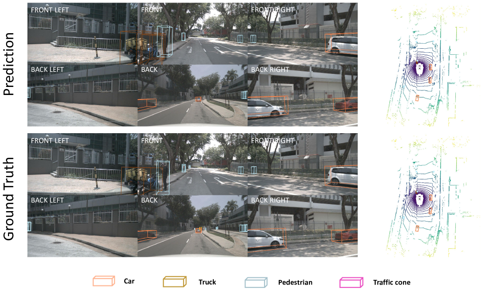
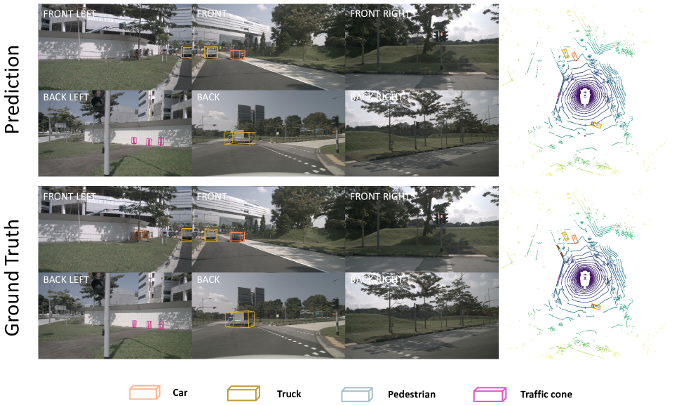
Figure 8: Visualizations (Part I): Given multi-camera images, our method dedicates to perform 3D object detection and BEV semantic segmentation.

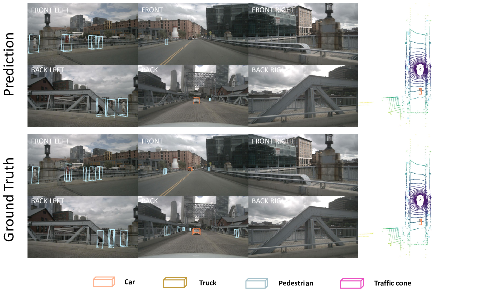
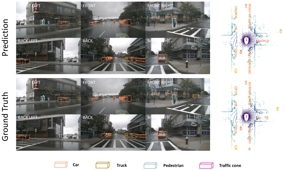
Figure 9: Visualizations (Part II): Given multi-camera images, our method dedicates to perform 3D object detection and BEV semantic segmentation.

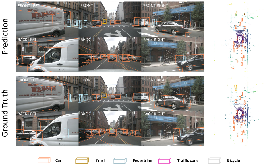
Figure 10: Visualizations (Part III): Given multi-camera images, our method dedicates to perform 3D object detection and BEV semantic segmentation.

We visualize our 3D object detection and BEV semantic segmentation results in Figure 8, Figure 9 and Figure 10.

Limitations and potential societal impact

Limitations

Since existing BEV based 3D object detection methods consider usually the Cartesian coordinate, there is a lacking of elaborately designed off-the-shelf LiDAR detection heads and corresponding tricks suitable for the Polar coordinate based methods as we propose here. That means there is some room for performance gain in head design, which will be one of the future works.

Societal impact

Our method can be used as the perception module for autonomous driving. However, our system is not perfect yet and hence not fully trustworthy in real-world deployment. Also, the current system is not exhaustively evaluated and tested due to limited resources as existing alternative works. Autonomous driving is still a largely immature field with many ongoing and unsolved matters including those complex legitimate issues, and many of those may be concerned with this work too.

Scale variance of objects on Polar BEV feature map

Although Polar BEV feature map could preserve rich features in non-far regions when compared with Cartesian BEV feature map, it has to overcome scale variance problem, a challenge which is not presented in Cartesian BEV feature map. The object scale variance lies in that the size of an object in the Polar BEV feature map could reduce increasingly when it moves away from the ego-vehicle. Here we give an example of objects moving far away from the ego-vehicle in radial direction and provide simple mathematical proof.

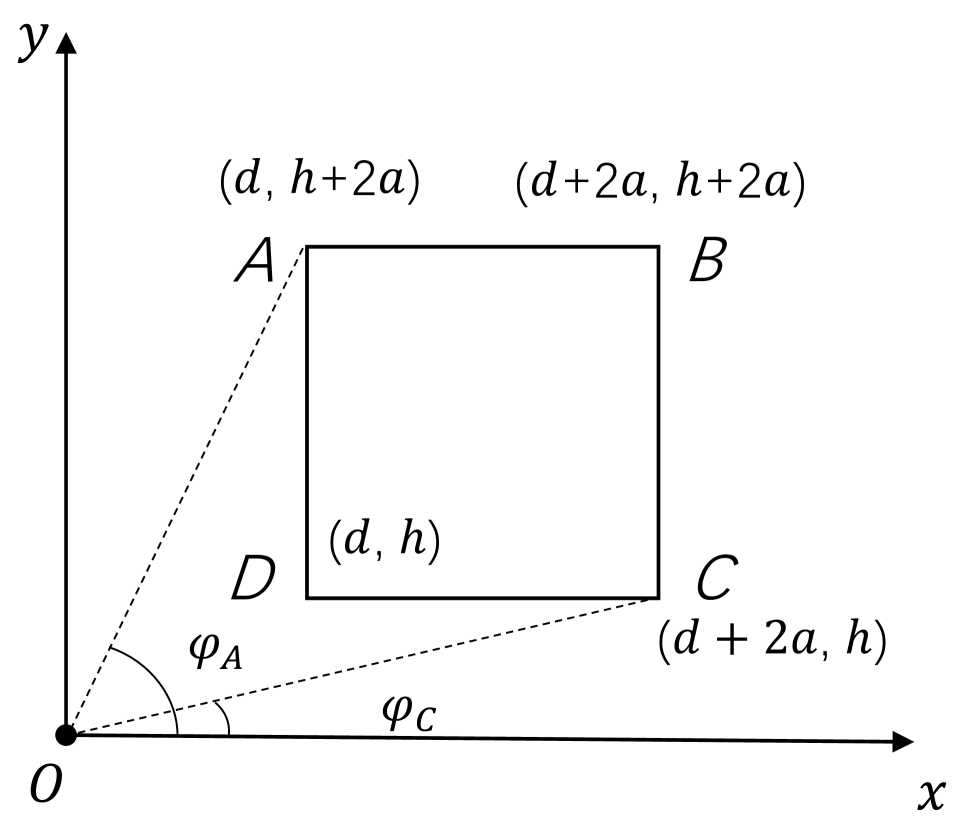
(a) Cartesian BEV feature map

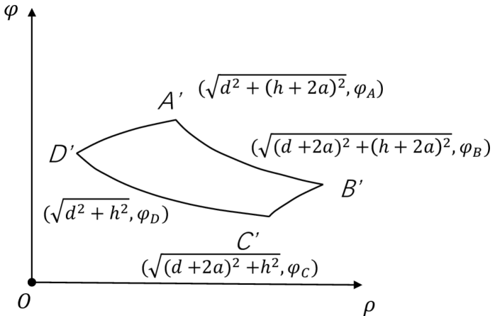
(b) Polar BEV feature map

Figure 7: Object on feature maps with different coordinates.

We consider the bounding box of an object as a square with length $2a$ ($a>0)$ and denote the object by $ABCD$ and $A’B’C’D’$ in the Cartesian and Polar BEV feature map, respectively (Figure 7(a) and 7(b)) .The occupied area of the object in the Polar BEV feature map is denoted by $S$. Note that the coordinate of $D$ is $(d,h)$, where $d\in[1,50],h\in[1,50]$, denoting the detection range.

Regarding $d$ as the only variable, we could prove $S(d)$ is monotonically decreasing functioned with $d$ by calculating $S^{\prime}(d)$.

First, the functions in Polar BEV feature map for the curve $D^{\prime}A^{\prime}$, $A^{\prime}B^{\prime}$, $B^{\prime}C^{\prime}$, and $C^{\prime}D^{\prime}$ are

$$\begin{split}&\varphi_{D^{\prime}A^{\prime}}(\rho,d)=\arctan\frac{\sqrt{\rho^{2}-d^{2}}}{d},\\ &\rho\in[\sqrt{d^{2}+h^{2}},\sqrt{d^{2}+(h+2a)^{2}}],\end{split}$$ (12)

$$\begin{split}&\varphi_{A^{\prime}B^{\prime}}(\rho,d)=\arctan\frac{h+2a}{\sqrt{\rho^{2}-(h+2a)^{2}}},\\ &\rho\in[\sqrt{d^{2}+(h+2a)^{2}},\sqrt{(d+2a)^{2}+(h+2a)^{2}}\end{split}$$ (13)

$$\begin{split}&\varphi_{B^{\prime}C^{\prime}}(\rho,d)=\arctan\frac{\sqrt{\rho^{2}-(d+2a)^{2}}}{d+2a},\\ &\rho\in[\sqrt{(d+2a)^{2}+h^{2}},\sqrt{(d+2a)^{2}+(h+2a)^{2}}]\end{split}$$ (14)

$$\begin{split}&\varphi_{C^{\prime}D^{\prime}}(\rho,d)=\arctan\frac{h}{\sqrt{\rho^{2}-h^{2}}},\\ &\rho\in[\sqrt{d^{2}+h^{2}},\sqrt{(d+2a)^{2}+h^{2}}]\end{split}$$ (15)

Thus, the area of curve $D^{\prime}A^{\prime}B^{\prime}C^{\prime}$ is

$$S(d) =\left(\int_{\sqrt{d^{2}+h^{2}}}^{\sqrt{d^{2}+(h+2a)^{2}}}\varphi_{D^{\prime}A^{\prime}}(\rho,d)d\rho+\right.$$ (5)

$$\left.\int_{\sqrt{d^{2}+(h+2a)^{2}}}^{\sqrt{(d+2a)^{2}+(h+2a)^{2}}}\varphi_{A^{\prime}B^{\prime}}(\rho,d)d\rho\right)$$

$$-\left(\int_{\sqrt{(d+2a)^{2}+h^{2}}}^{\sqrt{(d+2a)^{2}+(h+2a)^{2}}}\varphi_{B^{\prime}C^{\prime}}(\rho,d)d\rho+\right.$$

$$\left.\int_{\sqrt{d^{2}+h^{2}}}^{\sqrt{(d+2a)^{2}+h^{2}}}\varphi_{C^{\prime}D^{\prime}}(\rho,d)d\rho\right)$$

$$=\left(\int_{\sqrt{d^{2}+h^{2}}}^{\sqrt{d^{2}+(h+2a)^{2}}}\arctan\frac{\sqrt{\rho^{2}-d^{2}}}{d}d\rho+\right.$$

$$\left.\int_{\sqrt{d^{2}+(h+2a)^{2}}}^{\sqrt{(d+2a)^{2}+(h+2a)^{2}}}\arctan\frac{h+2a}{\sqrt{\rho^{2}-(h+2a)^{2}}}d\rho\right)$$

$$-\left(\int_{\sqrt{(d+2a)^{2}+h^{2}}}^{\sqrt{(d+2a)^{2}+(h+2a)^{2}}}\arctan\frac{\sqrt{\rho^{2}-(d+2a)^{2}}}{d+2a}d\rho+\right.$$

$$\left.\int_{\sqrt{d^{2}+h^{2}}}^{\sqrt{(d+2a)^{2}+h^{2}}}\arctan\frac{h}{\sqrt{\rho^{2}-h^{2}}}d\rho\right)$$

To proof $S(d)$ is monotonically decreasing functioned with $d$, we are going to show $S^{\prime}(d)<0.(d\in[1,50],h\in[1,50],a>0)$

First, we get $S^{\prime}(d)$ as follows:

$$S^{\prime}(d) =\left(\int_{\sqrt{d^{2}+h^{2}}}^{\sqrt{d^{2}+(h+2a)^{2}}}-\frac{1}{\sqrt{\rho^{2}-d^{2}}}d\rho+\right.$$ (6)

$$\left.\frac{d}{\sqrt{d^{2}+(h+2a)^{2}}}\arctan\frac{h+2a}{d}-\right.$$

$$\left.\frac{d}{\sqrt{d^{2}+h^{2}}}\arctan\frac{h}{d}\right)$$

$$+\left(\frac{d+2a}{\sqrt{(d+2a)^{2}+(h+2a)^{2}}}\arctan\frac{h+2a}{d+2a}-\right.$$

$$\left.\frac{d}{\sqrt{d^{2}+(h+2a)^{2}}}\arctan\frac{h+2a}{d}\right)$$

$$-\left(\int_{\sqrt{(d+2a)^{2}+h^{2}}}^{\sqrt{(d+2a)^{2}+(h+2a)^{2}}}-\frac{1}{\sqrt{\rho^{2}-(d+2a)^{2}}}d\rho+\right.$$

$$\left.\frac{d+2a}{\sqrt{(d+2a)^{2}+(h+2a)^{2}}}\arctan\frac{h+2a}{d+2a}-\right.$$

$$\left.\frac{d+2a}{\sqrt{(d+2a)^{2}+h^{2}}}\arctan\frac{h}{d+2a}\right)$$

$$-\left(\frac{d+2a}{\sqrt{(d+2a)^{2}+h^{2}}}\arctan\frac{h}{d+2a}-\right.$$

$$\left.\frac{d}{\sqrt{d^{2}+h^{2}}}\arctan\frac{h}{d}\right)$$

$$=\int_{\sqrt{d^{2}+h^{2}}}^{\sqrt{d^{2}+(h+2a)^{2}}}-\frac{1}{\sqrt{\rho^{2}-d^{2}}}d\rho-$$

$$\int_{\sqrt{(d+2a)^{2}+h^{2}}}^{\sqrt{(d+2a)^{2}+(h+2a)^{2}}}-\frac{1}{\sqrt{\rho^{2}-(d+2a)^{2}}}d\rho$$

$$=\ln\frac{\sqrt{(d+2a)^{2}+(h+2a)^{2}}+h+2a}{\sqrt{(d+2a)^{2}+h^{2}}+h}-$$

$$\ln\frac{\sqrt{d^{2}+(h+2a)^{2}}+h+2a}{\sqrt{d^{2}+h^{2}}+h}$$

Take $f(x)=\frac{\sqrt{x^{2}+(h+2a)^{2}}+h+2a}{\sqrt{x^{2}+h^{2}}+h},x\in[d,d+2a]$, we have

$$f^{\prime}(x) =\left(\frac{x}{\sqrt{x^{2}+(h+2a)^{2}}}(\sqrt{x^{2}+h^{2}}+h)-\right.$$ (7)

$$\left.\frac{x}{\sqrt{x^{2}+h^{2}}}(\sqrt{x^{2}+(h+2a)^{2}}+h+2a)\right)$$

$$\cdot(\sqrt{x^{2}+h^{2}}+h)^{2}$$

$$=\frac{x}{(\sqrt{x^{2}+h^{2}}+h)^{2}\sqrt{x^{2}+(h+2a)^{2}}\sqrt{x^{2}+h^{2}}}$$

$$\cdot\left[\sqrt{x^{2}+h^{2}}(\sqrt{x^{2}+h^{2}}+h)-\right.$$

$$\left.\sqrt{x^{2}+(h+2a)^{2}}(\sqrt{x^{2}+(h+2a)^{2}}+h+2a)\right]$$

$$=\frac{x}{(\sqrt{x^{2}+h^{2}}+h)^{2}\sqrt{x^{2}+(h+2a)^{2}}\sqrt{x^{2}+h^{2}}}$$

$$\cdot\left[q(h)-q(h+2a)\right]<0$$

where, $q(t)=\sqrt{x^{2}+t^{2}}(\sqrt{x^{2}+t^{2}}+t)$ is a monotonically increasing function in the domain $[h,h+2a]$ Obviously, $f(x)$ is a monotonically decreasing function with positive values in the domain $[d,d+2a]$. And $g(x)=\ln(x)$ is a monotonically increasing function in the positive field. Thus, $g(f(x)$ is monotonically decreasing functioned with $x$ in the domain $[d,d+2a]$, which means $g(f(d+2a))<g(f(d))$. Therefore, we have

$$S^{\prime}(d) =\ln\frac{\sqrt{(d+2a)^{2}+(h+2a)^{2}}+h+2a}{\sqrt{(d+2a)^{2}+h^{2}}+h}$$ (8)

$$-\ln\frac{\sqrt{d^{2}+(h+2a)^{2}}+h+2a}{\sqrt{d^{2}+h^{2}}+h}$$

$$=g(f(d+2a))-g(f(d))<0$$

So the occupied area of the object decreases when $d$ increases, and symmetrically, we could obtain the same conclusion for $h$. When objects move far away from the ego-vehicle in the radial direction, both $d$ and $h$ increase, thus $S$ will decrease too. For a generic object with arbitrary orientation, we could consider that it is formed by multiple small squares and the same conclusion can be drawn.

References

- Bewley et al. (2020) Bewley, A.; Sun, P.; Mensink, T.; Anguelov, D.; and Sminchisescu, C. 2020. Range conditioned dilated convolutions for scale invariant 3d object detection. arXiv preprint.
- Caesar et al. (2020) Caesar, H.; Bankiti, V.; Lang, A. H.; Vora, S.; Liong, V. E.; Xu, Q.; Krishnan, A.; Pan, Y.; Baldan, G.; and Beijbom, O. 2020. nuScenes: A multimodal dataset for autonomous driving. In CVPR.
- Can et al. (2021) Can, Y. B.; Liniger, A.; Paudel, D. P.; and Van Gool, L. 2021. Structured Bird’s-Eye-View Traffic Scene Understanding from Onboard Images. In ICCV.
- Carion et al. (2020) Carion, N.; Massa, F.; Synnaeve, G.; Usunier, N.; Kirillov, A.; and Zagoruyko, S. 2020. End-to-end object detection with transformers. In ECCV.
- Chen, Vora, and Beijbom (2021) Chen, Q.; Vora, S.; and Beijbom, O. 2021. PolarStream: Streaming Object Detection and Segmentation with Polar Pillars. In NeurIPS.
- Chitta, Prakash, and Geiger (2021) Chitta, K.; Prakash, A.; and Geiger, A. 2021. NEAT: Neural Attention Fields for End-to-End Autonomous Driving. In ICCV.
- Contributors (2020) Contributors, M. 2020. MMDetection3D: OpenMMLab next-generation platform for general 3D object detection. https://github.com/open-mmlab/mmdetection3d.
- Ding et al. (2020) Ding, M.; Huo, Y.; Yi, H.; Wang, Z.; Shi, J.; Lu, Z.; and Luo, P. 2020. Learning depth-guided convolutions for monocular 3d object detection. In CVPR.
- Guizilini et al. (2020) Guizilini, V.; Ambrus, R.; Pillai, S.; Raventos, A.; and Gaidon, A. 2020. 3D Packing for Self-Supervised Monocular Depth Estimation. In CVPR.
- He et al. (2016) He, K.; Zhang, X.; Ren, S.; and Sun, J. 2016. Deep residual learning for image recognition. In CVPR.
- Hu et al. (2021) Hu, A.; Murez, Z.; Mohan, N.; Dudas, S.; Hawke, J.; Badrinarayanan, V.; Cipolla, R.; and Kendall, A. 2021. FIERY: Future Instance Prediction in Bird’s-Eye View From Surround Monocular Cameras. In ICCV.
- Huang and Huang (2022) Huang, J.; and Huang, G. 2022. Bevdet4d: Exploit temporal cues in multi-camera 3d object detection. arXiv preprint.
- Lee et al. (2019) Lee, Y.; Hwang, J.-w.; Lee, S.; Bae, Y.; and Park, J. 2019. An energy and GPU-computation efficient backbone network for real-time object detection. In CVPR.
- Li et al. (2021) Li, Q.; Wang, Y.; Wang, Y.; and Zhao, H. 2021. HDMapNet: A Local Semantic Map Learning and Evaluation Framework. arXiv preprint.
- Li et al. (2022) Li, Z.; Wang, W.; Li, H.; Xie, E.; Sima, C.; Lu, T.; Yu, Q.; and Dai, J. 2022. BEVFormer: Learning Bird’s-Eye-View Representation from Multi-Camera Images via Spatiotemporal Transformers. arXiv preprint.
- Lin et al. (2017) Lin, T.-Y.; Goyal, P.; Girshick, R.; He, K.; and Dollár, P. 2017. Focal loss for dense object detection. In ICCV.
- Lin et al. (2014) Lin, T.-Y.; Maire, M.; Belongie, S.; Hays, J.; Perona, P.; Ramanan, D.; Dollár, P.; and Zitnick, C. L. 2014. Microsoft coco: Common objects in context. In ECCV.
- Lu et al. (2022) Lu, J.; Zhou, Z.; Zhu, X.; Xu, H.; and Zhang, L. 2022. Learning Ego 3D Representation as Ray Tracing. In ECCV.
- Ma et al. (2019) Ma, X.; Wang, Z.; Li, H.; Zhang, P.; Ouyang, W.; and Fan, X. 2019. Accurate monocular 3d object detection via color-embedded 3d reconstruction for autonomous driving. In ICCV.
- Park et al. (2021) Park, D.; Ambrus, R.; Guizilini, V.; Li, J.; and Gaidon, A. 2021. Is Pseudo-Lidar needed for Monocular 3D Object detection? In ICCV.
- Philion and Fidler (2020) Philion, J.; and Fidler, S. 2020. Lift, splat, shoot: Encoding images from arbitrary camera rigs by implicitly unprojecting to 3d. In ECCV.
- Rapoport-Lavie and Raviv (2021) Rapoport-Lavie, M.; and Raviv, D. 2021. It’s All Around You: Range-Guided Cylindrical Network for 3D Object Detection. In ICCV.
- Reading et al. (2021) Reading, C.; Harakeh, A.; Chae, J.; and Waslander, S. L. 2021. Categorical depth distribution network for monocular 3d object detection. In CVPR.
- Roddick and Cipolla (2020) Roddick, T.; and Cipolla, R. 2020. Predicting semantic map representations from images using pyramid occupancy networks. In CVPR.
- Roddick, Kendall, and Cipolla (2019) Roddick, T.; Kendall, A.; and Cipolla, R. 2019. Orthographic feature transform for monocular 3d object detection. In BMVC.
- Saha et al. (2022) Saha, A.; Maldonado, O. M.; Russell, C.; and Bowden, R. 2022. Translating Images into Maps. In ICRA.
- Tian et al. (2019) Tian, Z.; Shen, C.; Chen, H.; and He, T. 2019. Fcos: Fully convolutional one-stage object detection. In ICCV.
- Vaswani et al. (2017) Vaswani, A.; Shazeer, N.; Parmar, N.; Uszkoreit, J.; Jones, L.; Gomez, A. N.; Kaiser, Ł.; and Polosukhin, I. 2017. Attention is all you need. In NeurIPS.
- Wang et al. (2022a) Wang, T.; Xinge, Z.; Pang, J.; and Lin, D. 2022a. Probabilistic and geometric depth: Detecting objects in perspective. In CoRL.
- Wang et al. (2021) Wang, T.; Zhu, X.; Pang, J.; and Lin, D. 2021. Fcos3d: Fully convolutional one-stage monocular 3d object detection. In ICCV.
- Wang et al. (2019) Wang, Y.; Chao, W.-L.; Garg, D.; Hariharan, B.; Campbell, M.; and Weinberger, K. Q. 2019. Pseudo-lidar from visual depth estimation: Bridging the gap in 3d object detection for autonomous driving. In CVPR.
- Wang et al. (2022b) Wang, Y.; Guizilini, V. C.; Zhang, T.; Wang, Y.; Zhao, H.; and Solomon, J. 2022b. Detr3d: 3d object detection from multi-view images via 3d-to-2d queries. In CoRL.
- Xie et al. (2022) Xie, E.; Yu, Z.; Zhou, D.; Philion, J.; Anandkumar, A.; Fidler, S.; Luo, P.; and Alvarez, J. M. 2022. M^ 2BEV: Multi-Camera Joint 3D Detection and Segmentation with Unified Birds-Eye View Representation. arXiv preprint.
- Xu and Chen (2018) Xu, B.; and Chen, Z. 2018. Multi-level fusion based 3d object detection from monocular images. In CVPR.
- Yang et al. (2021) Yang, W.; Li, Q.; Liu, W.; Yu, Y.; Ma, Y.; He, S.; and Pan, J. 2021. Projecting Your View Attentively: Monocular Road Scene Layout Estimation via Cross-view Transformation. In CVPR.
- Yin, Zhou, and Krähenbühl (2021) Yin, T.; Zhou, X.; and Krähenbühl, P. 2021. Center-based 3D Object Detection and Tracking. In CVPR.
- You et al. (2019) You, Y.; Wang, Y.; Chao, W.-L.; Garg, D.; Pleiss, G.; Hariharan, B.; Campbell, M.; and Weinberger, K. Q. 2019. Pseudo-lidar++: Accurate depth for 3d object detection in autonomous driving. arXiv preprint.
- Zhang et al. (2020) Zhang, Y.; Zhou, Z.; David, P.; Yue, X.; Xi, Z.; Gong, B.; and Foroosh, H. 2020. Polarnet: An improved grid representation for online lidar point clouds semantic segmentation. In CVPR.
- Zhou, Wang, and Krähenbühl (2019) Zhou, X.; Wang, D.; and Krähenbühl, P. 2019. Objects as points. arXiv preprint.
- Zhu et al. (2021a) Zhu, X.; Su, W.; Lu, L.; Li, B.; Wang, X.; and Dai, J. 2021a. Deformable detr: Deformable transformers for end-to-end object detection. In ICLR.
- Zhu et al. (2021b) Zhu, X.; Zhou, H.; Wang, T.; Hong, F.; Ma, Y.; Li, W.; Li, H.; and Lin, D. 2021b. Cylindrical and asymmetrical 3d convolution networks for lidar segmentation. In CVPR.