Randomized K-FACs: Speeding up K-FAC with Randomized Numerical Linear Algebra

Abstract

k-fac is a successful tractable implementation of Natural Gradient for Deep Learning, which nevertheless suffers from the requirement to compute the inverse of the Kronecker factors (through an eigen-decomposition). This can be very time-consuming (or even prohibitive) when these factors are large. In this paper, we theoretically show that, owing to the exponential-average construction paradigm of the Kronecker factors that is typically used, their eigen-spectrum must decay. We show numerically that in practice this decay is very rapid, leading to the idea that we could save substantial computation by only focusing on the first few eigen-modes when inverting the Kronecker-factors. Importantly, the spectrum decay happens over a constant number of modes irrespectively of the layer width. This allows us to reduce the time complexity of k-fac from cubic to quadratic in layer width, partially closing the gap w.r.t. seng (another practical Natural Gradient implementation for Deep learning which scales linearly in width). Randomized Numerical Linear Algebra provides us with the necessary tools to do so. Numerical results show we obtain $\approx 2.5\times$ reduction in per-epoch time and $\approx 3.3\times$ reduction in time to target accuracy. We compare our proposed k-fac sped-up versions seng, and observe that for CIFAR10 classification with VGG16_bn we perform on par with it.

1 Introduction

Research in optimization for DL has lately focused on Natural Gradient (NG), owing to its desirable properties when compared to standard gradient [1, 2]. k-fac ([3]) is a tractable implementation which nevertheless suffers from the drawback of requiring the actual inverses of the Kronecker Factors (not just a linear solve). This computation scales cubically in layer width. When K-Factors are large (eg. for very wide fully-connected layers), k-fac becomes very slow. A fundamentally different practical implementation of NG without this problem has been proposed: seng [4] (uses matrix sketching [5] and empirical NG [2]). seng scales linearly in layer width, thus substantially outperforming k-fac for very wide nets.

In this paper, we provide a way to alleviate k-fac’s issue and make it competitive with seng, by partly closing the complexity gap. We begin by theoretically noting that the eigenspectrum of the K-Factors must decay rapidly, owing to their exponential-average (EA) construction paradigm. Numerical results of practically obtained eigen-spectrums show that in practice, the decay is much faster than the one implied by our worst-case scenario theoretical analysis. Using these observations, we employ randomized Numerical Linear Algebra (rNLA, [6]) to reduce the time complexity from cubic to quadratic in layer width. This gives us highly time-efficient approximation routes for K-Factors inversion, with minimal accuracy reduction. Numerically, our proposed methods speed up k-fac by $2.5\times$ and $3.3\times$ in terms of time per epoch and time to target accuracy respectively. Our algorithms outperform seng [4] (w.r.t. wall time) for moderate and high target test accuracy, but slightly underperform for very high test accuracy.

Related Work: The work of Tang et. al. (2021, [7]) is most related. However, their main approach is to construct a more efficient inversion of the regularized low-rank K-factors, without any rNLA. To make their approach feasible, they have to perform an EA over $A_{k}^{(l)}$ and $G_{k}^{(l)}$ rather than over $\bar{\mathcal{A}}_{k}^{(l)}$ and $\bar{\Gamma}_{k}^{(l)}$, as is standard (see Section 2.1). Our approach avoids this issue. Osawa et. al. (2020, [8]) presents some ideas to speed-up k-fac, but they are orthogonal to ours.

2 Preliminaries

Neural Networks (NNs): Our learning problem is

$$\min_{\theta}f(\theta):=\frac{1}{|\mathcal{D}|}\sum_{(x_{i},y_{i})\in\mathcal{D}}\big{(}-\log p(y_{i}|h_{\theta}(x_{i}))\big{)},$$ (1)

where $\mathcal{D}$ is the dataset containing input-target pairs $\{x_{i},y_{i}\}$, $\theta$ are the aggregated network parameters, $h_{\theta}(\cdot)$ is the neural network function (with $n_{L}$ layers), and $p(y|h_{\theta}(x_{i}))$ is the predictive distribution of the network (over labels - e.g. over classes), which is parameterized by $h_{\theta}(x_{i})$. We let $p_{\theta}(y|x):=p(y|h_{\theta}(x))$, $g_{k}:=\nabla_{\theta}f(\theta_{k})$, and note that we can express $g_{k}=[g_{k}^{(1)},...,g_{k}^{(n_{L})}]$, where $g_{k}^{(l)}$ is the gradient of parameters in layer $l$. We will always use a superscript to refer to the layer index and a subscript to refer to the optimization iteration index.

2.1 Fisher Information, Natural Gradient and K-FAC

The Fisher information is defined as

$$F_{k}:=F(\theta_{k}):=\mathbb{E}_{\begin{subarray}{c}x\sim\mathcal{D}\\ y\sim p_{\theta}(y|x)\end{subarray}}\biggl{[}\nabla_{\theta}\log p_{\theta}(y|x)\nabla_{\theta}\log p_{\theta}(y|x)^{T}\biggr{]}.$$ (2)

A NG descent (NGD) algorithm with stepsize $\alpha_{k}$ takes steps of the form $s^{(\text{NGD})}_{k}=-\alpha_{k}\nabla_{\text{NG}}f(\theta_{k})$, where $\nabla_{\text{NG}}f(\theta_{k})$ is the natural gradient (NG), defined as [1]

$$\nabla_{NG}f(\theta_{k}):=F_{k}^{-1}g_{k}.$$ (3)

In DL, the dimension of $F_{k}$ is very large, and $F_{k}$ can neither be stored nor used to complete a linear-solve. k-fac ([3]) is a practical implementation of the NGD algorithm which bypasses this problem by approximating $F_{k}$ as

$$F_{k}^{(\text{KFAC})}:=\text{blockdiag}\big{(}\{\mathcal{A}^{(l)}_{k}\otimes\Gamma^{(l)}_{k}\}_{l=1,...,n_{L}}\big{)},$$ (4)

where $\mathcal{A}^{(l)}_{k}:=A_{k}^{(l)}[A_{k}^{(l)}]^{T}$ and $\Gamma^{(l)}_{k}:=G_{k}^{(l)}[G_{k}^{(l)}]^{T}$ are the forward K-factor and backward K-factor respectively (of layer $l$ at iteration $k$) [3]. Each block corresponds to a layer and $\otimes$ denotes the Kronecker product. The exact K-Factors definition depends on the layer type (see [3] for FC layers, [9] for Conv layers). For our purpose, it is sufficient to state that $A_{k}^{(l)}\in\mathbb{R}^{d^{(l)}_{\mathcal{A}}\times n^{(l)}_{A}}$ and $G_{k}^{(l)}\in\mathbb{R}^{d^{(l)}_{\Gamma}\times n^{(l)}_{\Gamma}}$, with $n^{(l)}_{\mathcal{A}},n^{(l)}_{\Gamma}\propto n_{\text{BS}}$, where $n_{\text{BS}}$ is the batch size (further size details in [3, 9]).

Computing $(F_{k}^{(\text{KFAC})})^{-1}g_{k}$ can be done relatively efficiently in a block-wise fashion, since we have $(\mathcal{A}^{(l)}_{k}\otimes\Gamma^{(l)}_{k})^{-1}g_{k}^{(l)}=\text{vec}\big{(}[\Gamma^{(l)}_{k}]^{-1}\text{Mat}(g_{k}^{(l)})[\mathcal{A}^{(l)}_{k}]^{-1}\big{)}$, where $\text{vec}(\cdot)$ is the matrix vectorization operation and $\text{Mat}(\cdot)$ is its inverse. Note that since $\text{Mat}(g_{k}^{(l)})$ is a matrix, we need to compute the inverses of $\bar{\mathcal{A}}^{(l)}_{k}$ and $\bar{\Gamma}^{(l)}_{k}$ (eg. through an eigen-decomposition - and not just linear-solve with them). This is point is essential.

k-fac pseudo-code is shown in Algorithm 1. Note that in practice, instead of assembling $F_{k}^{(\text{KFAC})}$ as in equation (4), with the K-factors local to $\theta_{k}$ ($\mathcal{A}^{(l)}_{k}$ and $\Gamma^{(l)}_{k}$), we use an exponential average (EA) ($\bar{\mathcal{A}}^{(l)}_{k}$ and $\bar{\Gamma}^{(l)}_{k}$; see lines 4 and 8 in Algorithm 1). This aspect is important for our discussion in Section 3. In Algorithm 1 we initialize $\bar{\mathcal{A}}^{(l)}_{-1}:=I$ and $\bar{\Gamma}^{(l)}_{-1}:=I$. $\theta_{0}$ is initialized as typical [10].

1

2for $k=0,1,2,....$, with sampled batch $\mathcal{B}_{k}\subset\mathcal{D}$ do

3      

4      for $l=0,1,...,N_{L}$ do // Perform forward pass

5             Get $a^{(l)}_{k}$ and $A^{(l)}_{k}$

6            $\bar{\mathcal{A}}^{(l)}_{k}\leftarrow\rho\bar{\mathcal{A}}^{(l)}_{k-1}+(1-\rho)A^{(l)}_{k}[A^{(l)}_{k}]^{T}$ // Update fwd. EA K-factors

7            

8      Get $\tilde{f}(\theta_{k})$ ;

9        // The batch-estimate of $f(\theta_{k})$, from $a^{(l)}_{k}$

10      

11      for $l=N_{L},N_{L-1},...,1$ do // Perform backward pass

12             Get $g^{(l)}_{k}$ and $G^{(l)}_{k}$

13            $\bar{\Gamma}^{(l)}_{k}\leftarrow\rho\bar{\Gamma}^{(l)}_{k-1}+(1-\rho)G^{(l)}_{k}[G^{(l)}_{k}]^{T}$ // Update bwd. EA K-factors

14            

15      Get gradient $g_{k}=\big{[}\big{(}g^{(1)}_{k}\big{)}^{T},...\big{(}g^{(N_{L})}_{k}\big{)}^{T}\big{]}^{T}$

16      for $l=0,1,...,N_{L}$ do // Compute k-fac step:

17             // Get Eig of $\bar{\mathcal{A}}^{(l)}_{k}$ and $\bar{\Gamma}^{(l)}_{k}$ for inverse application

18             $U^{(l)}_{A,k}D^{(l)}_{A,k}\big{(}U^{(l)}_{A,k}\big{)}^{T}=\text{eig}(\bar{\mathcal{A}}^{(l)}_{k})$ ; $U^{(l)}_{\Gamma,k}D^{(l)}_{\Gamma,k}\big{(}U^{(l)}_{\Gamma,k}\big{)}^{T}=\text{eig}(\bar{\Gamma}^{(l)}_{k})$

19            // Use Eigs to apply K-FAC EA matrices inverses to $g^{(l)}_{k}$

20            

21            $M^{(l)}_{k}=\text{Mat}(g^{(l)}_{k})U^{(l)}_{A,k}(D^{(l)}_{A,k}+\lambda I)^{-1}\big{(}U^{(l)}_{A,k}\big{)}^{T}$

22            $S^{(l)}_{k}=U^{(l)}_{\Gamma,k}(D^{(l)}_{\Gamma,k}+\lambda I)^{-1}\big{(}U^{(l)}_{\Gamma,k}\big{)}^{T}M^{(l)}_{k}$ ; $s^{(l)}_{k}=\text{vec}(S^{(l)}_{k})$

23      $\theta_{k+1}=\theta_{k}-\alpha_{k}[(s_{k}^{(1)})^{T},...,(s_{k}^{(N_{L})})^{T}]^{T}$ // Take K-FAC step

24      

25

Algorithm 1 k-fac [3]

2.1.1 Key notes on Practical Considerations

In practice, we update the Kronecker-factors and recompute their eigendecompositions (“inverses”) only every few tens/hundreds of steps (update period $T_{K,U}$, inverse computation period $T_{K,I}$) [3]. Typically, we have $T_{K,I}>T_{K,U}$. As we began in Algorithm 1, we formulate our discussion for the case when $T_{K,I}=T_{K,U}=1$. We do this purely for simplicity of exposition. Extending our simpler discussion to the case when these operations happen at a smaller frequency is trivial, and does not modify our conclusions. Our practical implementations use the standard practical procedures.

2.2 Randomized SVD (RSVD)

Before we begin diving into rNLA, we note that whenever we say rsvd, or qr, we always refer to the thin versions unless otherwise specified. Let us focus on the arbitrary matrix $X\in\mathbb{R}^{m\times n}$. For convenience, assume for this section that $m>n$ (else we can transpose $X$). Consider the svd of $X$

$$X\mathrel{\stackrel{{\scriptstyle\makebox[0.0pt]{\mbox{\tiny SVD}}}}{{\,=\,}}}U_{X}\Sigma_{X}V_{X}^{T},$$ (5)

and assume $\Sigma_{X}$ is sorted decreasingly. It is a well-known fact that the best rank-$r$ approximation of $X$ is given by $U_{X}[:,:r]\Sigma_{X}[:r,:r]V_{X}[:,:r]^{T}$ [6]. The idea behind randomized svd is to obtain these first $r$ singular modes without computing the entire (thin) svd of $X$, which is $\mathcal{O}(mn^{2})$ time complexity. Algorithm 2 shows the rsvd algorithm alongside with associated time complexities. We omit the derivation and error analysis for brevity (see [6] for details).

1 Input: $X\in\mathbb{R}^{m\times n}$, target rank $r<\min(m,n)$, oversampling param. $r_{l}\leq n-r$

2Output: Approximation of the first $r$ singular modes of $X$

3Sample Gaussian Matrix $\Omega\in\mathbb{R}^{n\times(r+l)}$ // $\mathcal{O}(n(r+l))$ flops

4

5Compute $X\Omega$ // $\mathcal{O}(mn(r+l))$ flops

6

7$QR=\text{QR\_decomp}(X\Omega)$ // $\mathcal{O}(m(r+l)^{2})$ flops

8

9$B:=Q^{T}X\in\mathbb{R}^{(r+l)\times n}$ // $\mathcal{O}(nm(r+l))$ flops

10

11Compute Full SVD (i.e. not the thin one) of $B^{T}$, and transpose it to recover $B\,\,\,\mathrel{\stackrel{{\scriptstyle\makebox[0.0pt]{\mbox{\tiny FULL-SVD}}}}{{\,\,\,\,\,\,=\,\,\,\,\,\,}}}\,\,\,U_{B}\Sigma_{B}V_{B}^{T}$ // $\mathcal{O}(n^{2}(r+l))$ flops

12

13$\tilde{U}_{X}=QU_{B}$; $\tilde{\Sigma}_{X}=\Sigma_{B}[:r,:r]$; $\tilde{V}_{X}=V_{B}[:,:r]$ // $\mathcal{O}(m(r+l)^{2})$ flops

14

Return $\tilde{U}_{X}\in\mathbb{R}^{m\times r}$, $\tilde{\Sigma}_{X}\in\mathbb{R}^{r\times r}$, $\tilde{V}_{X}\in\mathbb{R}^{n\times r}$

Algorithm 2 Randomized svd (rsvd) [6]

The returned quantities, $\tilde{U}_{X}\in\mathbb{R}^{m\times r}$, $\tilde{\Sigma}_{X}\in\mathbb{R}^{r\times r}$, $\tilde{V}_{X}\in\mathbb{R}^{n\times r}$ are approximations for $U_{X}[:,:r]$, $\Sigma_{X}[:r,:r]$ and $V_{X}[:,:r]$ respectively - which is what we were after. These approximations are relatively good with high probability, particularly when the singular values spectrum is rapidly decaying [6]. The total complexity of rsvd is $\mathcal{O}(n^{2}(r+r_{l})+mn(r+r_{l}))$ - significantly better than the complexity of svd $\mathcal{O}(m^{2}n)$ when $r+r_{l}\ll\min(m,n)$. We will see how we can use this to speed up k-fac in Section 4.1. Note the presence of the over-sampling parameter $r_{l}$, which helps with accuracy at minimal cost. This $r_{l}$ will appear in many places. Finally, we note that $Q$ is meant to be a skinny-tall orthonormal matrix s.t. $\left\lVert X-QQ^{T}X\right\rVert_{F}$ is “small”. There are many ways to obtain $Q$, but in lines 3-4 of Algorithm 2 we presented the simplest one for brevity (see [6] for details). In practice we perform the power iteration in line 4 $n_{\text{pwr-it}}$ times (possibly more than once).

2.2.1 RSVD Error Components

Note that there are two error components when using the returned quantities of an rsvd to approximate a matrix. The first component is the truncation error - which is the error we would have if we computed the svd and then truncated. The second error is what we will call projection error, which is the error between the rank-$r$ svd-truncated $X$ and the rsvd reconstruction of $X$ (which appears due to the random Gaussian matrix).

2.2.2 RSVD for Square Symmetric PSD matrices

When our matrix $X$ is square-symmetric PSD (the case we will fall into) we have $m=n$, $U_{X}=V_{X}$, and the svd (5) is also the eigen-value decomposition. As rsvd brings in significant errors, Algorithm 2 will return $\tilde{U}_{X}\neq\tilde{V}_{X}$ even in this case. Thus, we have to choose between using $\tilde{V}_{X}$ and $\tilde{U}_{X}$ (or any combination of these). A key point to note is that $\tilde{V}_{X}$ approximates $V_{X}[:,:r]$ better than $\tilde{U}_{X}$ approximates $U_{X}[:,:r]$ [12]. Thus using $\tilde{V}_{X}\tilde{\Sigma}_{X}\tilde{V}_{X}^{T}$ as the rank-$r$ approximation to $X$ is preferable. This is what we do in practice, and it gives us virtually zero projection error.

2.3 Symmetric Randomized EVD (SREVD)

When $X$ is square-symmetric PSD we have $m=n$, $U_{X}=V_{X}$, and the svd (5) is also the eigen-value decomposition (evd). In that case, we can exploit the symmetry to reduce the computation cost of obtaining the first $r$ modes. srevd is shown in Algorithm 3. The returned quantities, $\tilde{U}_{X}\in\mathbb{R}^{m\times r}$ and $\tilde{\Sigma}_{X}\in\mathbb{R}^{r\times r}$ are approximations for $U_{X}[:,:r]$ and $\Sigma_{X}[:r,:r]$ respectively - which is what we were after. The same observations about $Q$ that we made in Section 2.2 also apply here.

1 Input: Square, Symmetric PSD matrix $X\in\mathbb{R}^{n\times n}$

2Output: Approximation of the first $r$ eigen-modes of $X$

3Sample Gaussian Matrix $\Omega\in\mathbb{R}^{n\times(r+l)}$ // $\mathcal{O}(n(r+l))$ flops

4

5Compute $X\Omega$ // $\mathcal{O}(n(r+l))$ flops

6

7$QR=\text{QR\_decomp}(X\Omega)$ // $\mathcal{O}(n(r+l)^{2})$ flops

8

9Compute $C=Q^{T}XQ$ // $\mathcal{O}(n^{2}(r+l))$ flops

10

11$P_{C}D_{C}P_{C}^{T}=\text{Eigen\_decomp}(C)$ // $\mathcal{O}((r+l)^{3})$ flops

12

13$\tilde{U}_{X}=QP_{C}$; $\tilde{\Sigma}_{X}\in\mathbb{R}^{r\times r}$ // $\mathcal{O}(n(r+l)^{2})$ flops

14

Return $\tilde{U}_{X}\in\mathbb{R}^{n\times r}$, $\tilde{\Sigma}_{X}\in\mathbb{R}^{r\times r}$

Algorithm 3 Symmetric Randomized evd (srevd) [6]

The complexity is still $\mathcal{O}(n^{2}(r+l))$ as with rsvd, but the full-SVD of $(Q^{T}X)^{T}$ ($\mathcal{O}(n^{2}(r+l))$ complexity) is now replaced by a matrix-matrix multiplication of $\mathcal{O}(n(r+l)^{2})$ and a virtually free eigenvalue decomposition. However, note that by projecting both the columnspace and the rowspace of $X$ onto $Q$, we are losing accuracy because we are essentially not able to obtain the more accurate $\tilde{V}_{X}$ as we did with rsvd. That is because we have $P_{C}=Q^{T}U_{X}$, and thus we can only obtain $\tilde{U}_{X}=QQ^{T}U_{X}$ but not $\tilde{V}_{X}$. Consequently, the projection error is larger for srevd than for rsvd, although the turncation error is the same.

3 The Decaying Eigen-spectrum of K-Factors

3.0.1 Theoretical Investigation

Let $\lambda_{M}$ be the max. eigenvalue of the arbitrary EA Kronecker-factor

$$\bar{\mathcal{M}_{k}}=(1-\rho)\sum_{i=-\infty}^{k}\rho^{k-i}M_{i}M_{i}^{T},$$ (6)

with $M_{i}\in\mathbb{R}^{d_{M}\times n_{M}}$, $n_{M}\propto n_{\text{BS}}$. We now look at an upperbound on the number of eigenvalues that satisfy $\lambda_{i}\geq\epsilon\lambda_{M}$ (for some assumed $\alpha\in(0,1)$, chosen $\epsilon\in(0,1)$, and “sufficiently large” given $d_{M}$). Proposition 3.1 gives the result.

Proposition 3.1: Bounds describing eigenvalue decay of $\bar{\mathcal{M}_{k}}$.

Consider the $\bar{\mathcal{M}}_{k}$ in (6), let $\lambda_{M}$ be its maximum eigenvalue, and let us choose some $\epsilon\in(0,1)$. Assume the maximum singular value of $M_{i}$ is $\leq\sigma_{M}$ $\forall k$, and that we have $\lambda_{M}\geq\alpha\sigma_{M}^{2}$ for some fixed $\alpha\in(0,1)$. Then, we have that at most $\min(r_{\epsilon}n_{M},d_{M})$ eigenvalues of $\bar{\mathcal{M}_{k}}$ are above $\epsilon\lambda_{M}$, with

$$r_{\epsilon}=\left\lceil{{\log(\alpha\epsilon)}/{\log(\rho)}}\right\rceil.$$ (7)

Proof. We have $\bar{\mathcal{M}_{k}}=\bar{\mathcal{M}}_{\text{old}}+\bar{\mathcal{M}}_{\text{new}}$ with $\bar{\mathcal{M}}_{\text{old}}:=(1-\rho)\sum_{i=-\infty}^{k-r}\rho^{k-i}M_{i}M_{i}^{T}$, and $\bar{\mathcal{M}}_{\text{new}}:=(1-\rho)\sum_{i=k-r+1}^{k}\rho^{k-i}M_{i}M_{i}^{T}$.

First, let us find $r$ s.t. the following desired upper-bound holds:

$$\lambda_{\text{Max}}(\bar{\mathcal{M}}_{\text{old}})\leq\alpha\epsilon\sigma_{M}^{2}.$$ (8)

Let $\rho_{C}:=(1-\rho)$. By using $\left\lVert\cdot\right\rVert_{2}=\lambda_{\text{Max}}(\cdot)$ for s.p.s.d. arguments, we have

$$\lambda_{\text{Max}}\big{(}\bar{\mathcal{M}}_{\text{old}}\big{)}\leq\rho_{C}\sum_{i=-\infty}^{k-r}\rho^{k-i}\lambda_{\text{Max}}\big{(}M_{i}M_{i}^{T}\big{)}\leq\rho_{C}\sigma_{M}^{2}\rho^{r}\sum_{i=0}^{\infty}\rho^{i}=\sigma_{M}^{2}\rho^{r}.$$ (9)

Thus, in order to get (8) to hold, we can set $\sigma_{M}^{2}\rho^{r}\leq\epsilon\alpha\sigma_{M}^{2}$ from (9). That is, we must have $r\geq\log(\alpha\epsilon)/\log(\rho)$. Thus, choosing

$$r:=r_{\epsilon}:=\left\lceil{{\log(\alpha\epsilon)}/{\log(\rho)}}\right\rceil$$ (10)

ensures (8) holds. Now, clearly, $\text{rank}\big{(}\bar{\mathcal{M}}_{\text{new}}\big{)}\leq n_{M}r$, so $\bar{\mathcal{M}}_{\text{new}}$ has at most $n_{M}r$ non-zero eigenvalues. Using $\bar{\mathcal{M}_{k}}=\bar{\mathcal{M}}_{\text{old}}+\bar{\mathcal{M}}_{\text{new}}$ and the upperbound (8) (which holds for our choice of $r=r_{\epsilon}$) gives that $\bar{\mathcal{M}_{k}}$ has at most $n_{M}r_{\epsilon}$ eigenvalues above $\alpha\epsilon\sigma_{M}^{2}$. But by assumption the biggest eigenvalue of $\bar{\mathcal{M}_{k}}$ satisfies $\lambda_{M}\geq\alpha\sigma_{M}^{2}$. Thus, at most $n_{M}r_{\epsilon}$ of $\bar{\mathcal{M}_{k}}$ satisfy $\lambda_{i}\geq\epsilon\lambda_{M}$. This completes the proof. $\square$

Proposition 3.1 gives the notable result that the number of modes we need to save for a target $\epsilon$ depends only on our tolerance level $\epsilon$ (practically $\epsilon=1/33$) and on the batch-size (through $n_{M}\propto n_{\text{BS}}$), but not on $d_{M}$. To see this, note that Proposition 3.1 gives that the number of modes to save is in principle $r_{\epsilon}n_{M}=\left\lceil{{\log(\alpha\epsilon)}/{\log(\rho)}}\right\rceil n_{M}$, which does not depend on $d_{M}$. Thus, increasing $d_{M}$ (past $r_{\epsilon}n_{M}$) does not affect how many modes we need to compute (to ensure we only ignore eigenvalues below $\epsilon\lambda_{\text{max}}$). Intuitively, this means we can construct approaches which scale better in $d_{M}$ than evd: the evd computes $d_{M}$ modes when we only really need a constant (w.r.t. $d_{M}$) number of modes! This is good news for k-fac: its bottleneck was the scaling of evd with the net width ($d_{M}$’s)!

The assumption about $\lambda_{M}$ may seem artificial, but holds well in practice. A more in depth analysis may avoid it. Plugging realistic values of $\epsilon=0.03$, $\alpha=0.1$ and $\rho=0.95$, $n_{M}=n_{\text{BS}}=256$ (holds for FC layers) in Proposition 3.1 tells us we have to retain at least $n_{M}r_{\epsilon}=29184$ eigenmodes to ensure we only ignore eigenvalues satisfying $\lambda_{i}\leq 10^{-1.5}\lambda_{M}$. Clearly, 29184 is very large, and Proposition 3.1 is not directly useful in practice. However, it does ensure us that the eigenspectrum of the EA K-Factors must have a form of which implies we only really need to keep a constant number (w.r.t. $d_{M}$) of eigenmodes. We now show numerically that this decay is much more rapid than inferred by our worst-case analysis here.

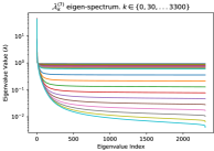
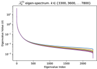
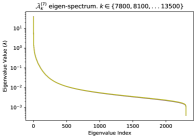
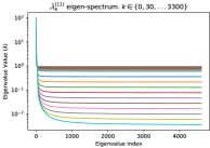
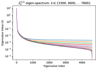
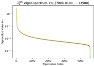
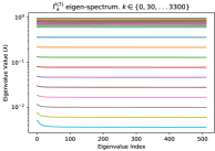
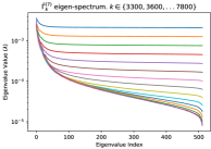
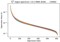
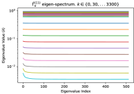
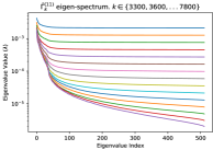
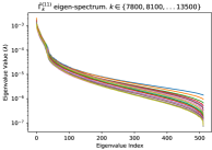
Figure 1: K-Factors eigen-spectrum: layers 7 and 11 of VGG16_bn for CIFAR10 dataset. Each curve represents the spectrum for a specific step $k$.

3.0.2 Numerical Investigation of K-Factors Eigen-Spectrum

We ran k-fac for 70 epochs, with the specifications outlined in Section 5 (but with $T_{K,U}=T_{K,I}=30$). We saved the eigen-spectrum every 30 steps if $k<300$, and every 300 steps otherwise. Only results for layers 7 and 11 are shown for the sake of brevity, but they were virtually identical for all other layers. We see that for low $k$, all eigenvalues are close to unity, which is due to $\bar{\mathcal{A}}$ and $\bar{\Gamma}$ being initialized to the identity. However, the spectrum rapidly develops a strong decay (where more than 1.5 orders of magnitude are decayed within the first 200 eigenvalues). It takes $\bar{\mathcal{A}}$ about 500 steps (that is about 2.5 epochs) and $\bar{\Gamma}$ about 5100 steps (26 epochs) to develop this strong spectrum decay. We consider 1.5 orders of magnitude a strong decay because the K-Factors regularization that we found to work best is around $\lambda_{\text{max}}/10$ (for which any eigenvalue below $\lambda_{\text{max}}/33$ can be considered zero without much accuracy loss). Thus, truncating our K-Factors to an $r\approx 220$ worked well in practice. Importantly, once the spectrum reaches its equilibrium state, we get this 1.5 orders of magnitude decay within 200 modes irrespective of the size of the K-factor ($d_{M}$). This aligns with the intuition provided by Proposition 3.1.

4 Speeding Up EA K-Factors Inversion

We now present two approaches for speeding up k-fac, which avoid the typically used evd of the K-factors through obtaining approximations to the low-rank truncations of these evds. The ideas are similar in spirit and presented in the order of increasing computational saving (and reducing accuracy).

4.1 Proposed Optimizer: RSVD K-FAC (RS-KFAC)

Instead of computing the eigen-decompositions of the EA-matrices (K-Factors) $\bar{\mathcal{A}}$ and $\bar{\Gamma}$ (in line 12 of Algorthm 1; of time complexity $\mathcal{O}(d_{\mathcal{A}}^{3})$ and $\mathcal{O}(d_{\Gamma}^{3})$), we could settle for using a rank $r$ rsvd approximation:

$$\bar{\mathcal{A}}\,\mathrel{\stackrel{{\scriptstyle\makebox[0.0pt]{\mbox{\tiny RSVD}}}}{{\,\,\approx\,\,}}}\,\tilde{U}_{A}\tilde{D}_{A}\tilde{U}_{A}^{T},\,\,\,\text{and }\,\,\,\bar{\Gamma}\,\mathrel{\stackrel{{\scriptstyle\makebox[0.0pt]{\mbox{\tiny RSVD}}}}{{\,\,\approx\,\,}}}\,\tilde{U}_{\Gamma}\tilde{D}_{\Gamma}\tilde{U}_{\Gamma}^{T},$$ (11)

where $\tilde{U}_{A}\in\mathbb{R}^{d_{\mathcal{A}}\times r}$, $\tilde{U}_{\Gamma}\in\mathbb{R}^{d_{\Gamma}\times r}$, and $\tilde{D}_{A},\tilde{D}_{\Gamma}\in\mathbb{R}^{r\times r}$.

Using this trick, we reduce the computation cost of line 12 in Algorithm 1 from $\mathcal{O}(d_{\mathcal{A}}^{3}+d_{\Gamma}^{3})$ to $\mathcal{O}((d_{\mathcal{A}}^{2}+d_{\Gamma}^{2})(r+r_{l}))$ when using an oversampling parameter $r_{l}$. This is a dramatic reduction since we can choose $(r+r_{l})\ll\min(d_{\mathcal{A}},d_{\Gamma})$ with minimal truncation error, as we have seen in Section 3. As discussed in Section 2.3, for rsvd the projection error is virtually zero, and thus small truncation error means our rsvd approach will give very close results to using the full eigenspectrum. Once we have the approximate low-rank truncations, we estimate

$$(\bar{\Gamma}+\lambda I)^{-1}V\approx(\tilde{U}_{\Gamma,r}\tilde{D}_{\Gamma,r}\tilde{U}_{\Gamma,r}^{T}+\lambda I)^{-1}V,$$ (12)

where $\lambda$ is the regularization parameter (applied to K-factors), and then compute

$$\begin{split}(\tilde{U}_{\Gamma,r}\tilde{D}_{\Gamma,r}\tilde{U}_{\Gamma,r}^{T}+\lambda I)^{-1}V=\tilde{U}_{\Gamma,r}\biggl{[}(\tilde{D}_{\Gamma,r}+\lambda I)^{-1}-\frac{1}{\lambda}I\biggr{]}\tilde{U}_{\Gamma,r}^{T}V+\frac{1}{\lambda}V.\end{split}$$ (13)

We use (13) because its r.h.s. is cheaper to compute than its l.h.s. Note that computing (13) has complexity $\mathcal{O}(rd_{\Gamma}+2rd_{\Gamma}^{2})$, which is better than computing line 15 of Algorithm 1 of complexity $\mathcal{O}(d_{\Gamma}^{3})$. We take a perfectly analogous approach for $V(\bar{\mathcal{A}}+\lambda I)^{-1}$. The rs-kfac algorithm is obtained by replacing lines 10 - 15 in Algorithm 1 with the for loop shown in Algorithm 4. Over-all rs-kfac scales like $\mathcal{O}(d_{M}^{2}(r+r_{l}))$ (setting $d_{M}=d_{\mathcal{A}}^{(l)}=d_{\Gamma}^{(l)}$, $\forall l$ for simplicity).

1 Replace lines 10 - 15 in Algorithm 1 with:

2for $l=0,1,...,N_{L}$ do

3       // Get RSVD of $\bar{\mathcal{A}}^{(l)}_{k}$ and $\bar{\Gamma}^{(l)}_{k}$ for inverse application

4       $\tilde{U}^{(l)}_{A,k}\tilde{D}^{(l)}_{A,k}(\tilde{V}^{(l)}_{A,k})^{T}=\text{RSVD}(\bar{\mathcal{A}}^{(l)}_{k})$; $\tilde{U}_{\Gamma,k}^{(l)}\tilde{D}_{\Gamma,k}^{(l)}(\tilde{V}^{(l)}_{\Gamma,k})^{T}=\text{RSVD}(\bar{\Gamma}^{(l)}_{k})$

5      // Use RSVD factors to approx. apply inverse of K-FAC matrices

6      

7      $J^{(l)}_{k}=\text{Mat}(g_{k}^{(l)})$

8      $M^{(l)}_{k}=J^{(l)}_{k}\tilde{V}^{(l)}_{A,k}\big{[}(\tilde{D}^{(l)}_{A,k}+\lambda I)^{-1}-\frac{1}{\lambda}I\big{]}(\tilde{V}^{(l)}_{A,k})^{T}+\frac{1}{\lambda}J^{(l)}_{k}$

9      $S^{(l)}_{k}=\tilde{V}^{(l)}_{\Gamma,k}\biggl{[}(\tilde{D}^{(l)}_{\Gamma,k}+\lambda I)^{-1}-\frac{1}{\lambda}I\biggr{]}(\tilde{V}^{(l)}_{\Gamma,k})^{T}M^{(l)}_{k}+\frac{1}{\lambda}M^{(l)}_{k}$

10      $s^{(l)}_{k}=\text{vec}(S^{(l)}_{k})$

11

Algorithm 4 rs-kfac (our first proposed algorithm)

Note that the RSVD subroutine in line 4 of Algorithm 4 may be executed using the rsvd in Algorithm 2, but using different rsvd implementations would not significantly change our discussion. As we have discussed in Section 2.3.1, even though $\tilde{U}^{(l)}_{A,k}$ should equal $\tilde{V}^{(l)}_{A,k}$ since $\bar{\mathcal{A}}_{k}^{(l)}$ is square s.p.s.d., the rsvd algorithm returns two (somewhat) different matrices, of which the more accurate one is the “V-matrix”. The same observation also applies to $\Gamma$-related quantities.

4.2 Proposed Optimizer: SREVD K-FAC (SRE-KFAC)

Instead of using rsvd in line 4 of Algorithm 4, we can exploit the symmetry and use srevd (e.g. with Algorithm 3). This would reduce the computation cost of that line by a constant factor, altough the computational complexity would be the same: $\mathcal{O}\big{(}(d_{\mathcal{A}}^{2}+d_{\Gamma}^{2})(r+r_{l})\big{)}$. However, this cost reduction comes at the expense of reduced accuracy, because srevd has significant projection error (unlike rsvd; recall Section 2.3). We refer to this algorithm as sre-kfac and briefly present it in Algorithm 5. Note that in line 4 of Algorithm 5 we assign $\tilde{V}\leftarrow\tilde{U}$ to avoid rewriting lines 7-8 of Algorithm 4 with $\tilde{V}$’s replaced by $\tilde{U}^{\prime}s$. Over-all sre-kfac scales like $\mathcal{O}(d_{M}^{2}(r+r_{l}))$ (setting $d_{M}=d_{\mathcal{A}}^{(l)}=d_{\Gamma}^{(l)}$, $\forall l$ for simplicity of exposition).

1 Replace lines lines 3 - 4 in Algorithm 4 with:

2// Get SREVD of $\bar{\mathcal{A}}^{(l)}_{k}$ and $\bar{\Gamma}^{(l)}_{k}$ for inverse application

3

4$\tilde{U}^{(l)}_{A,k}\tilde{D}^{(l)}_{A,k}(\tilde{U}^{(l)}_{A,k})^{T}=\text{SREVD}(\bar{\mathcal{A}}^{(l)}_{k})$; $\tilde{U}_{\Gamma,k}^{(l)}\tilde{D}_{\Gamma,k}^{(l)}(\tilde{U}^{(l)}_{\Gamma,k})^{T}=\text{SREVD}(\bar{\Gamma}^{(l)}_{k})$

$\tilde{V}^{(l)}_{A,k}=\tilde{U}^{(l)}_{A,k}$; $\tilde{V}^{(l)}_{\Gamma,k}=\tilde{U}^{(l)}_{\Gamma,k}$

Algorithm 5 sre-kfac (our second proposed algorithm)

4.3 Direct Idea Transfer to Other Applications

Application to ek-fac: We can apply the method directly to ek-fac (a k-fac improvement; [13]) as well.

Application to kld-wrm algorithms: Our idea can be directly applied to the kld-wrm family (see [14]) when k-fac is used as an implementation “platform”. Having a smaller optimal $\rho$ ($0.5$ as opposed to $0.95$), kld-wrm instantiations may benefit more from our porposed ideas, as they are able to use even lower target-ranks in the rsvd (or srevd) for the same desired accuracy. To see this, consider setting $\rho:=0.5$ (instead of $\rho=0.95$) in the practical calculation underneath Proposition 3.1. Doing so reduces the required number of retained eigenvalues down to $2304$ from $29184$.

4.4 Partly Closing the Complexity Gap between K-FAC and SENG

It is important to realise that this section gives us more than a way of significantly speeding K-FAC for large net widths (at negligible accuracy loss). It tells us that (based on the Discussion in Section 3 and Proposition 3.1) the scaling of $\mathcal{O}(d_{M}^{3})$ with layer width is not inherent to K-FAC (at least not when $d_{M}\gg n_{\text{BS}}$), and that we can obtain scaling of $\mathcal{O}(d_{M}^{2})$ for K-FAC at practically no accuracy loss.

This opportunity conceptually arises in a simple way. Roughly speaking, we have much less information in the K-factor estimate (scales with $n_{\text{BS}}$; and we cannot take too large batch-sizes) than would be required to estimate it accurately given its size $d_{M}\times d_{M}$ (when $d_{M}\gg n_{\text{BS}}$). Thus, whether the true K-factor has strong eigen-spectrum decay or not does not matter, our EA estimates are bound to exhibit it. So what causes a problem actually solves another: we cannot accurately estimate the K-factors for large $d_{M}$ given our bacth-size limitation - but this puts us in a place where our approximate decomposition/inversion computations which scale like $\mathcal{O}(d_{M}^{2})$ are virtually as good as the exact methods which scale like $\mathcal{O}(d_{M}^{3})$.

This brings K-FAC practically closer to the computational scaling of SENG (the more succesful practical NG implementation) To see this, note that we have $\mathcal{O}(d_{M}^{3})$ for K-FAC, $\mathcal{O}(d_{M}^{2})$ for Randomized K-FACs, and $\mathcal{O}(d_{M})$ for SENG. Conceptually, SENG has better scaling as it exploits this lack of information to speed-up computation by removing unnecesary ones. We hereby in this paper implicitly show that we can do a similar thing for K-FAC and obtain a better scaling with $d_{M}$!

5 Numerical Results: Proposed Algorithms Performance

We now numerically compare rs-kfac and sre-kfac with k-fac (the baseline we improve upon) and seng (another NG implementation which typically outperforms k-fac; see [4]). We did not test sgd, as this underpeforms seng (see Table 4 in [4]). We consider the CIFAR10 dataset with a modified version of batch-normalized VGG16 (VGG16_bn). All experiments ran on a single NVIDIA Tesla V100-SXM2-16GB GPU. The accuracy we refer to is always test accuracy.

5.0.1 Implementation Details

For seng, we used the implementation from the official github repo with the hyperparameters directly recommended by the authors for the problem at hand (via email). k-fac was slightly adapted from alecwangcq’s github. Our proposed solvers were built on that code. For k-fac, rs-kfac and sre-kfac we performed manual tuning. We found that no momentum, weight_decay = 7e-04, $T_{K,U}=10$, and $\rho=0.95$, alongside with the schedules $T_{K,I}(n_{\text{ce}})=50-20\mathbb{I}_{n_{\text{ce}}\geq 20}$, $\lambda_{K}(n_{\text{ce}})=0.1-0.05\mathbb{I}_{n_{\text{ce}}\geq 25}-0.04\mathbb{I}_{n_{\text{ce}}\geq 35}$, $\alpha_{k}(n_{ce})=0.3-0.1\mathbb{I}_{n_{ce}\geq 2}-0.1\mathbb{I}_{n_{ce}\geq 3}-0.07\mathbb{I}_{n_{ce}\geq 13}-0.02\mathbb{I}_{n_{ce}\geq 18}-0.007\mathbb{I}_{n_{ce}\geq 27}-0.002\mathbb{I}_{n_{ce}\geq 40}$ (where $n_{\text{ce}}$ is the number of the current epoch) worked best for all three k-fac based solvers. The hyperparameters specific to rs-kfac and sre-kfac were set to $n_{\text{pwr-it}}=4$, $r(n_{\text{ce}})=220+10\mathbb{I}_{n_{\text{ce}}\geq 15}$, $r_{l}(n_{\text{ce}})=10+\mathbb{I}_{n_{ce}\geq 22}+\mathbb{I}_{n_{\text{ce}}\geq 30}$. We set $n_{\text{BS}}=256$ throughout. We implemented all our k-fac-based algorithms in the empirical NG spirit (using $y$ from the given labels when computing the backward K-factors rather than drawing $y\sim p(y|h_{\theta}(x))$; see [2] for details). We performed 10 runs of 50 epochs for each $\{$solver, batch-size$\}$ pair.

Table 1: CIFAR10 VGG16_bn results summary. All solvers reached $91.5\%$ accuracy within the allocated 50 epochs for 10 out of 10 runs. Some solvers did not reach $92\%$ accuracy on all of their 10 runs, and this is shown in the sixth column of the table. Columns 2-4 show the time to get to a specific test accuracy. The fifth column shows time per epoch. All times are in seconds and presented in the form: mean $\pm$ standard deviation. For time per epoch, statistics are obtained across 500 samples (50 epochs $\times$ 10 runs). For times to a specific accuracy, statistics are obtained based only on the runs where the solver indeed reached the target accuracy (eg. for $92\%$, the 5 successful runs are used for k-fac). The last column of the table shows number of epochs to get to $92\%$ accuracy (results format is analogous to the ones of column 4).

	$t_{acc\geq 90\%}$	$t_{acc\geq 91.5\%}$	$t_{acc\geq 92\%}$	$t_{\text{epoch}}$	Runs hit $92\%$	$\mathcal{N}_{\text{acc}\geq 92\%}$
seng	$673.6\pm 34.4$	$693.2\pm 28.2$	$718.1\pm 26.0$	$16.6\pm 0.4$	10 out of 10	$43.3\pm 0.9$
k-fac	$1449\pm 8.7$	$1971\pm 225$	$2680\pm 636$	$75.5\pm 3.4$	5 out of 10	$35.4\pm 8.3$
rs-kfac	$445.8\pm 10.9$	$600.7\pm 4.9$	$732.6\pm 153.1$	$32.6\pm 0.9$	10 out of 10	$23.0\pm 4.7$
sre-kfac	$439.4\pm 28.5$	$582.2\pm 24.1$	$785.3\pm 155.6$	$30.0\pm 0.4$	7 out of 10	$26.3\pm 5.1$

5.0.2 Results Discussion

Table 1 shows important summary statistics. We see that the time per epoch is $\approx 2.4\times$ lower for our solvers than for k-fac. This was expected given we reduce time complexity from cubic to quadratic in layer width! In accordance with our discussion in Section 4.2, we see that sre-kfac is slightly faster per epoch than rs-kfac. Surprisingly, we see that the number of epochs to a target accuracy (at least for $92\%$) is also smaller for rs-kfac and sre-kfac than for k-fac. This indicates that dropping the low-eigenvalue modes does not seem to hinder optimization progress, but provide a further benefit instead. As a result, the time to a specific target accuracy is improved by a factor of $3$ - $4\times$ when using rs-kfac or sre-fac as opposed to k-fac. Note that sre-kfac takes more epochs to reach a target accuracy than rs-kfac. This is due sre-kfac further introducing a projection error compared to rs-kfac (see Section 4.2). For the same reason, rs-kfac always achieves $92\%$ test accuracy while sre-kfac only does so 7 out of 10 times. Surprisingly, k-fac reached $92\%$ even fewer times. We believe this problem appeared in k-fac based solvers due to a tendency to overfit, as can be seen in Figure 2.

When comparing to seng, we see that our proposed k-fac improvements perform slightly better for $91\%$ and $91.5\%$ target test accuracy, but slightly worse for $92\%$. We believe this problem will vanish if we can fix the over-fit of our k-fac based solvers. Overall, the numerical results show that our proposed speedups give substantially better implementations of k-fac, with time-to-accuracy speed-up factors of $\approx 3.3\times$. Figure 2 shows an in-depth view of our results.

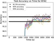
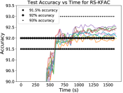
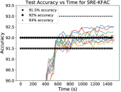
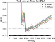
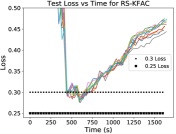
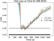
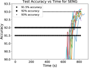
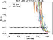
Figure 2: CIFAR10 with VGG16_bn test loss and test accuracy results.

6 Conclusion

We theoretically observed that the eigen-spectrum of the K-Factors must decay, owing to the associated EA construction paradigm. We then looked at numerical results on CIFAR10 and saw that the decay was much more rapid than predicted by our theoretical worst-case analysis. We then noted that the small eigenvalues are “washed away” by the standard K-Factor regularization. This led to the idea that, with minimal accuracy loss, we may replace the full eigendecomposition performed by k-fac with rNLA algorithms which only approximate the strongest few modes. We implicitly answer the question: how many modes?

Importantly, the eigen-spectrum decay was shown (theoretically and numerically) to be such that we only really need to keep a constant number of modes when maintaining a fixed, very good accuracy, irrespectively of what the layer width is! This allowed us to reduce the time complexity from $\mathcal{O}(d_{M}^{3})$ for k-fac down to $\mathcal{O}(d_{M}^{2}(r+r_{l}))$ for Randomized K-FACs, where $r$ and $r_{l}$ are constant w.r.t. $d_{M}$ for a fixed desired spectrum cut-off tolerance (for a generic K-factor with layer width $d_{M}$). We have seen that this complexity reduction from $\mathcal{O}(d_{M}^{3})$ to $\mathcal{O}(d_{M}^{2})$ partly closes the gap between k-fac and seng (which scales like $\mathcal{O}(d_{M})$).

We discussed theoretically that rsvd is more expensive but also more accurate than srevd, and the numerical performance of the corresponding optimizers confirmed this. Numerical results show we speed up k-fac by a factor of $2.3\times$ in terms of time per epoch, and even had a gain in per-epoch performance. Consequently, target test accuracies were reached about $3.3\times$ faster in terms of wall time. Our proposed k-fac speedups also outperformed the state of art seng (on a problem where it is much faster than k-fac; [4]) for $91\%$ and $91.5\%$ target test accuracy in terms of both epochs and wall time. For $92.0\%$ our proposed algorithms only mildly underperformed seng. We argued this could be resolved.

Future work: developing probabilistic theory about eigenspectrum decay which better reconciles numerical results, refining the rs-kfac and sre-kfac algorithms, and layer-specific adaptive selection mechanism for target rank.

6.0.1 Acknowledgments

Thanks to Jaroslav Fowkes and Yuji Nakatsukasa for useful discussions. I am funded by the EPSRC CDT in InFoMM (EP/L015803/1) together with Numerical Algorithms Group and St. Anne’s College (Oxford).

References

- [1] Amari, S. I. Natural gradient works efficiently in learning, Neural Computation, 10(20), pp. 251-276 (1998).
- [2] Martens, J. New insights and perspectives on the natural gradient method, arXiv:1412.1193 (2020).
- [3] Martens, J.; Grosse, R. Optimizing neural networks with Kronecker-factored approximate curvature, arXiv:1503.05671 (2015).
- [4] Yang, M.; Xu, D; Wen, Z.; Chen, M.; Xu, P. Sketchy empirical natural gradient methods for deep learning, arXiv:2006.05924 (2021).
- [5] Tropp, J. A.; Yurtsever, A.; Udell, M.; Cevher, V. Practical Sketching Algorithms for Low-Rank Matrix approximation, arXiv:1609.00048 (2017).
- [6] Halko N.; Martinsson P.G.; Tropp J. A. Finding structure with randomness: Probabilistic algorithms for constructing approximate matrix decompositions (2011).
- [7] Tang, Z.; Jiang, F.; Gong, M.; Li, H.; Wu, Y.; Yu, F.; Wang, Z.; Wang, M. SKFAC: Training Neural Networks with Faster Kronecker-Factored Approximate Curvature, IEEE/CVF Conference on Computer Vision and Pattern Recognition, (2021).
- [8] Osawa, K.; Yuichiro Ueno, T.; Naruse, A.; Foo, C.-S.; Yokota, R. Scalable and practical natural gradient for large-scale deep learning, arXiv:2002.06015 (2020).
- [9] Grosse, R.; Martens J. A Kronecker-factored approximate Fisher matrix for convolution layers, arXiv:1602.01407 (2016).
- [10] Murray, M.; Abrol, V.; Tanner, J. Activation function design for deep networks: linearity and effective initialisation, in arXiv:2105.07741, (2021).
- [11] Mazeika M. The Singular Value Decomposition and Low Rank Approximation.
- [12] Saibaba, A. K. Randomized subspace iteration: Analysis of canonical angles and unitarily invariant norms, arXiv:1804.02614 (2018).
- [13] Gao, K.-X.; Liu X.-L.; Huang Z.-H.; Wang, M.; Want S.; Wang, Z.; Xu, D.; Yu, F. Eigenvalue-corrected NG Based on a New Approximation, arXiv:2011.13609 (2020).
- [14] Puiu, C. O. Rethinking Exponential Averaging of the Fisher, arXiv:2204.04718 (2022).