Two A5 modular symmetries for Golden Ratio 2 mixing

Abstract

We present a model of leptonic mixing based on two $A_{5}$ modular symmetries using the Weinberg operator. The two modular symmetries are broken to the respective diagonal $A_{5}$ subgroup. At the effective level, the model behaves as a model with a single $A_{5}$ modular flavour symmetry, but with two moduli. Using both as stabilisers, different residual symmetries are preserved, leading to golden ratio mixing that is perturbed by a rotation.

I Introduction

Flavour symmetries are a promising solution to the flavour problem of the Standard Model (SM). Non-Abelian discrete symmetries are particularly suited to explain leptonic mixing, and have been explored frequently in the literature. Some of the most employed flavour symmetries are $S_{3}$, $A_{4}$, $S_{4}$ and $A_{5}$, which can be taken as modular symmetries $\Gamma_{2}\simeq S_{3}$ Kobayashi:2018vbk ; Kobayashi:2018wkl ; Okada:2019xqk ; Mishra:2020gxg ; Du:2020ylx , $\Gamma_{3}\simeq A_{4}$  Feruglio:2017spp ; Criado:2018thu ; Kobayashi:2018scp ; Okada:2018yrn ; Novichkov:2018yse ; Nomura:2019jxj ; Nomura:2019yft ; Ding:2019zxk ; Zhang:2019ngf ; Okada:2019mjf ; Nomura:2019lnr ; Asaka:2019vev ; Nomura:2019xsb ; Kobayashi:2019gtp ; Wang:2019xbo ; Okada:2020dmb ; Ding:2020yen ; Behera:2020sfe ; Nomura:2020opk ; Nomura:2020cog ; Behera:2020lpd ; Asaka:2020tmo ; Nagao:2020snm ; Hutauruk:2020xtk ; deMedeirosVarzielas:2021pug , $\Gamma_{4}\simeq S_{4}$ Penedo:2018nmg ; Novichkov:2018ovf ; deMedeirosVarzielas:2019cyj ; King:2019vhv ; Kobayashi:2019mna ; Okada:2019lzv ; Kobayashi:2019xvz ; Wang:2019ovr ; Wang:2020dbp , and $\Gamma_{5}\simeq A_{5}$ Novichkov:2018nkm ; Ding:2019xna .

Models employing multiple modular symmetries deMedeirosVarzielas:2019cyj ; King:2019vhv , deMedeirosVarzielas:2021pug have some advantages. As described in deMedeirosVarzielas:2019cyj , introducing the generic mechanism for using multiple modular symmetries, it allows models to be built based on residual symmetries, left unbroken by distinct moduli stabilisers. The preserved residual symmetries then lead to the realisation of different mass textures in the charged lepton and neutrino sectors in modular flavour models without flavons.

As an example, a $S_{4}$ flavour model featuring TM1 mixing Varzielas:2012pa is constructed in an elegant manner from multiple $S_{4}$ modular symmetries in deMedeirosVarzielas:2019cyj ; King:2019vhv , $S_{4}$ flavour models arise featuring e.g. TM1 mixing Varzielas:2012pa , from multiple $S_{4}$ modular symmetries, whereas in deMedeirosVarzielas:2021pug , multiple $A_{4}$ modular symmetries result in an $A_{4}$ model leading to TM2 mixing Grimus:2008tt .

In this paper, we construct a model that uses two $A_{5}$ modular symmetries in order to obtain the golden ratio mixing plus a rotation between the first and the third columns, using the Weinberg operator to generate the neutrino masses. This is akin to the models with multiple $S_{4}$ modular symmetries in King:2019vhv ; deMedeirosVarzielas:2019cyj . We refer also to Novichkov:2018nkm , where models with a single $A_{5}$ modular symmetry but with two moduli (using the Weinberg operator) generate the neutrino masses. The model that uses some fixed points of the modular fields lead to the same mixing we are going to discuss here, although that is not explicit in Novichkov:2018nkm . At high energies, the model is based in two modular symmetries, $A_{5}^{l}$ and $A_{5}^{\nu}$, with modulus fields denoted by $\tau_{l}$ and $\tau_{\nu}$, respectively. After the modulus fields acquire different VEV’s, different mass textures are realised in the charged lepton and neutrino sectors.

We will start by introducing some properties of the $A_{5}$ modular symmetry group. Subsequently, the various possibilities of a golden ratio mixing and a rotation among two of its columns are investigated and concluded that only a rotation between the first and third columns is compatible with the $3\sigma$ confidence interval from NuFit. Only then the explicit model will be introduced.

In Section II we briefly review the framework of multiple modular symmetries. In Section III we describe the $A_{5}$ modular symmetry and respective stabilisers associated to residual symmetries. In Section IV, the golden ratio mixing and variations are introduced and their compatibility with NuFit data verified. In Section V we present the model for GR2 mixing. We conclude in Section VI.

II Modular symmetries - an introduction

In this section we define the modular groups, modular forms, and review the framework introduced in deMedeirosVarzielas:2019cyj .

II.1 Modular group and modular forms

$\overline{\Gamma}$, the modular group, consists in all linear fractional transformations $\gamma$ acting on the complex modulus $\tau$ ($\tau$ in the upper-half complex plane, i.e. $Im(\tau)>0$):

$$\gamma:\tau\rightarrow\gamma\tau=\frac{a\tau+b}{c\tau+d}.$$ (1)

$a,b,c,d$ are integers with $ad-bc=1$.

Often, $2\times 2$ matrices represent these transformations:

$$\overline{\Gamma}=\left\{\begin{pmatrix}a&b\\ c&d\end{pmatrix}/\{\pm 1\},~{}a,b,c,d\in\mathbb{Z},~{}ad-bc=1\right\}.$$ (2)

As $\gamma$ and $-\gamma$ correspond to the same element, the group $\overline{\Gamma}$ is isomorphic to $PSL(2,\mathbb{Z})=SL(2,\mathbb{Z})/\mathbb{Z}_{2}$, with $SL(2,\mathbb{Z})$ being the group of $2\times 2$ matrices with integer entries and unit determinant.

The set of generators, $S_{\tau}$ and $T_{\tau}$, with $S_{\tau}^{2}=(S_{\tau}T_{\tau})^{3}=1$ generates the modular group. We take:

$$S_{\tau}:\tau\rightarrow-\frac{1}{\tau},~{}T_{\tau}:\tau\rightarrow\tau+1$$ (3)

which are represented, in matrix form

$$S_{\tau}=\begin{pmatrix}0&1\\ -1&0\end{pmatrix},~{}T_{\tau}=\begin{pmatrix}1&1\\ 0&1\end{pmatrix}.$$ (4)

We continue now to the subgroups $\overline{\Gamma}(N)$ of $\overline{\Gamma}$. These are obtained by taking the integer entries of the matrices modulo $N$:

$$\overline{\Gamma}(N)=\left\{\begin{pmatrix}a&b\\ c&d\end{pmatrix}\in PSL(2,\mathbb{Z}),~{}\begin{pmatrix}a&b\\ c&d\end{pmatrix}=\begin{pmatrix}1&0\\ 0&1\end{pmatrix}~{}(mod~{}\text{N})\right\}.$$ (5)

These subgroups are infinite, even though they are discrete for a given $N$. In turn, the quotient groups obtained by taking $\Gamma_{N}=\overline{\Gamma}/\overline{\Gamma}(N)$ are finite. They are referred to as the finite modular groups. For $N\leq 5$, these groups are isomorphic to the popular flavour symmetry groups mentioned already: $\Gamma_{2}\simeq S_{3}$, $\Gamma_{3}\simeq A_{4}$, $\Gamma_{4}\simeq S_{4}$, $\Gamma_{5}\simeq A_{5}$. The finite modular groups can be obtained by imposing $T_{\tau}^{N}=1$, meaning that $\tau=\tau+N$.

The Modular forms of a given modular weight $2k$ and for a fixed $N$ (the level) are holomorphic functions of $\tau$ that transform in a well-defined way under action by elements of $\overline{\Gamma}(N)$:

$$f(\gamma\tau)=(c\tau+d)^{2k}f(\tau),~{}\gamma=\begin{pmatrix}a&b\\ c&d\end{pmatrix}\in\overline{\Gamma}(N),$$ (6)

$k$ is here a non-negative integer, $N$ defines the underlying group (due to the modulo $N$), and we note that we will only consider even weights. The modular forms are invariant under transformations by $\overline{\Gamma}(N)$, up to the complex factor of $(c\tau+d)^{2k}$, but they do transform under the quotient group $\Gamma_{N}$.

Having fixed the level $N=5$, modular forms of a given weight $2k$ span a linear space of finite dimension $\mathcal{M}_{2k}(\overline{\Gamma}(5))$. The dimension of these linear spaces for $A_{5}$ is given by $10k+1$. Without loss of generality we select a basis in the linear space $\mathcal{M}_{2k}(\overline{\Gamma}(N))$ where the modular forms transform under $\Gamma_{N}$ with unitary representations $\rho$ of $\Gamma_{N}$:

$$f_{i}(\gamma\tau)=(c\tau+d)^{2k}\rho(\tilde{\gamma})_{ij}f_{j}(\tau),~{}\tilde{\gamma}\in\text{equivalence class of }\gamma\in\bar{\Gamma}\text{ in }\Gamma_{N}.$$ (7)

In the following sections, we will use $\gamma$ for $\tilde{\gamma}$, although this is the notation also used for the modular transformation under which the superpotential transforms.

II.2 Models with multiple modular symmetries

We now take into consideration multiple modular symmetries $\overline{\Gamma}^{1}$, $\overline{\Gamma}^{2}$, $\ldots$, $\overline{\Gamma}^{M}$. $\tau_{J}$ is the modulus field for the respective $\overline{\Gamma}^{J}$, $J=1,\ldots,M$. The transformations are:

$$\gamma_{J}:\tau_{J}\rightarrow\gamma_{J}\tau_{J}=\frac{a_{J}\tau_{J}+b_{J}}{c_{J}\tau_{J}+d_{J}}.$$ (8)

We generalise for each $J$ and obtain each $\Gamma_{N_{J}}^{J}$ for $J=1,\ldots,M$ by taking the quotient group. The integers $N_{J}$ can in general be distinct for each $J$.

Considering now a model invariant under the full group, the action is

$$S=\int d^{4}xd^{2}\theta d^{2}\overline{\theta}~{}K(\phi_{i},\overline{\phi}_{i};\tau_{1},\ldots,\tau_{M},\overline{\tau}_{1},\ldots,\overline{\tau}_{M})+\left(\int d^{4}xd^{2}\theta~{}W(\phi_{i};\tau_{1},\ldots,\tau_{M})+h.c.\right).$$ (9)

Under $\overline{\Gamma}^{J}$ for $J=1,\ldots,M$ the Kähler potential $K$ transforms at most by a Kähler transformation and the superpotential $W$ stays invariant:

$$K(\phi_{i},\overline{\phi}_{i};\tau_{1},\ldots,\tau_{M},\overline{\tau}_{1},\ldots,\overline{\tau}_{M}) \rightarrow K(\phi_{i},\overline{\phi}_{i};\tau_{1},\ldots,\tau_{M},\overline{\tau}_{1},\ldots,\overline{\tau}_{M})+f(\phi_{i};\tau_{1},\ldots,\tau_{M})+\overline{f}(\overline{\phi}_{i};\overline{\tau}_{1},\ldots,\overline{\tau}_{M})$$ (10)

$$W(\phi_{i};\tau_{1},\ldots,\tau_{M},\overline{\tau}_{1},\ldots,\overline{\tau}_{M}) \rightarrow W(\phi_{i};\tau_{1},\ldots,\tau_{M},\overline{\tau}_{1},\ldots,\overline{\tau}_{M}).$$ (11)

We assume here the minimal form of the Kähler potential. The effects of considering non-minimal forms of the Kähler potential may be relevant and are discussed in Chen:2019ewa ; Feruglio:2021dte . The superpotential is in general a function of the modulus $\tau_{i}$ and superfields $\phi_{i}$ and the expansion in powers of the superfields takes the form

$$W(\phi_{i};\tau_{1},\ldots,\tau_{M})=\sum_{n}\sum_{\{i_{1},\ldots,i_{n}\}}\sum_{(I_{Y,1},\ldots,I_{Y,M})}~{}(Y_{(I_{Y,1},\ldots,I_{Y,M})}\phi_{i_{1}}\ldots\phi_{i_{n}})_{\mathbf{1}}.$$ (12)

For the superpotential to be invariant under any modular transformation $\gamma_{1},\ldots,\gamma_{M}$ in $\overline{\Gamma}^{1}$, $\overline{\Gamma}^{2}$, $\ldots$, $\overline{\Gamma}^{M}$, the couplings $Y_{(I_{Y,1},\ldots,I_{Y,M})}$ must be multiplet modular forms, and the superfields $\phi_{i}$ must transform as

$$\phi_{i}(\tau_{1},\ldots,\tau_{M}) \rightarrow\phi_{i}(\gamma_{1}\tau_{1},\ldots,\gamma_{M}\tau_{M})$$

$$= \prod_{J=1,\ldots,M}(c_{J}\tau_{J}+d_{J})^{-2k_{i,J}}\bigotimes_{J=1,\ldots,M}\rho_{I_{i,J}}(\gamma_{J})~{}\phi_{i}(\tau_{1},\ldots,\tau_{M})$$ (13)

$$Y_{(I_{Y,1},\ldots,I_{Y,M})}(\tau_{1},\ldots,\tau_{M}) \rightarrow Y_{(I_{Y,1},\ldots,I_{Y,M})}(\gamma_{1}\tau_{1},\ldots,\gamma_{M}\tau_{M})$$

$$= \prod_{J=1,\ldots,M}(c_{J}\tau_{J}+d_{J})^{2k_{Y,J}}\bigotimes_{J=1,\ldots,M}\rho_{I_{Y,J}}(\gamma_{J})~{}Y_{(I_{Y,1},\ldots,I_{Y,M})}(\tau_{1},\ldots,\tau_{M}).$$ (14)

where $-2k_{i,J}$ is the modular weight of $\phi_{i}$, $I_{i,J}$ is the irrep of $\Gamma_{N}$ under which $\phi_{i}$ transforms, $2k_{Y,J}$ is the modular weight of $Y_{I_{Y,J}}$, $I_{Y,J}$ is the irrep of $\Gamma_{N}$ under which $Y_{I_{Y,J}}$ transforms and $\rho_{I_{i,J}}(\gamma)$ and $\rho_{I_{Y,J}}(\gamma)$ are the unitary representation matrices of $\gamma_{J}$ with $\gamma_{J}\in\Gamma_{N_{J}}^{J}$. Naturally, the superpotential can only be invariant when $k_{Y,J}=k_{i_{1},J}+\ldots+k_{i_{n},J}$, and when there is a trivial singlet in $I_{Y,J}\times I_{i_{1},J}\times\ldots\times I_{i_{n},J}$ for all $J=1,\ldots,M$.

III Modular $A_{5}$ symmetry and residual symmetries

In the following subsection the $A_{5}$ symmetry group is introduced, including some of its main properties as the modular forms of level 5 and its stabilisers which apply for the specific case of $A_{5}$ modular symmetries. The stabilisers for the modular groups from $N=2$ to $5$, can be found in deMedeirosVarzielas:2020kji .

III.1 Modular $A_{5}$ symmetry and modular forms of level 5

The group $A_{5}$ is the group of even permutations of 5 objects and has 60 elements. It is generated by two operators $S_{\tau}$ and $T_{\tau}$ obeying

$$S_{\tau}^{2}=(S_{\tau}T_{\tau})^{3}=T_{\tau}^{5}=1.$$ (15)

This group has one singlet $\mathbf{1}$, two triplets $\mathbf{3}$ and $\mathbf{3^{\prime}}$, one quadruplet $\mathbf{4}$ and one quintuplet $\mathbf{5}$ as its irreducible representations. The irreducible representations of the generators and the multiplication rules for the irreducible representations can be found in Appendix A.

The Yukawa couplings in a theory that is invariant under a $\Gamma_{5}\sim A_{5}$ symmetry are going to be modular forms of level 5. The eleven linearly independent weight 2 modular forms of level 5 form a quintuplet $Y_{\mathbf{5}}^{(2)}=(Y_{1},Y_{2},Y_{3},Y_{4},Y_{5})$ of $A_{5}$, a triplet $\mathbf{3}$ $Y_{\mathbf{3}}^{(2)}=(Y_{6},Y_{7},Y_{8})$ and a triplet $\mathbf{3^{\prime}}$ $Y_{\mathbf{3^{\prime}}}^{(2)}=(Y_{9},Y_{10},Y_{11})$. These modular functions can be expressed in terms of the third theta function (see Appendix B for more details). The modular forms of higher weight are generated starting from these eleven modular forms of weight 2.

The space of the weight 4 modular forms of level 5 has dimension 21 and decomposes into a singlet $\mathbf{1}$, one triplet $\mathbf{3}$, one triplet $\mathbf{3^{\prime}}$, a quadruplet $\mathbf{4}$ and two quintuplets $\mathbf{5}$. Using the weight 2 modular forms, one obtains the following expressions for the weight 4 modular forms Novichkov:2018nkm :

$$Y^{(4)}_{\mathbf{1}} =Y_{1}^{2}+2Y_{3}Y_{4}+2Y_{2}Y_{5},$$ (16)

$${Y^{(4)}_{\mathbf{3}}} =\begin{pmatrix}-2Y_{1}Y_{6}+\sqrt{3}Y_{5}Y_{7}+\sqrt{3}Y_{2}Y_{8}\\ \sqrt{3}Y_{2}Y_{6}+Y_{1}Y_{7}-\sqrt{6}Y_{3}Y_{8}\\ \sqrt{3}Y_{5}Y_{6}-\sqrt{6}Y_{4}Y_{7}+Y_{1}Y_{8}\\ \end{pmatrix},$$ (17)

$${Y^{(4)}_{\mathbf{3^{\prime}}}} =\begin{pmatrix}\sqrt{3}Y_{1}Y_{6}+Y_{5}Y_{7}+Y_{2}Y_{8}\\ Y_{3}Y_{6}-\sqrt{2}Y_{2}Y_{7}-\sqrt{2}Y_{4}Y_{8}\\ Y_{4}Y_{6}-\sqrt{2}Y_{3}Y_{7}-\sqrt{2}Y_{5}Y_{8}\\ \end{pmatrix},$$ (18)

$${Y^{(4)}_{\mathbf{4}}} =\begin{pmatrix}2Y_{4}^{2}+\sqrt{6}Y_{1}Y_{2}-Y_{3}Y_{5}\\ 2Y_{2}^{2}+\sqrt{6}Y_{1}Y_{3}-Y_{4}Y_{5}\\ 2Y_{5}^{2}-Y_{2}Y_{3}+\sqrt{6}Y_{1}Y_{4}\\ 2Y_{3}^{2}-Y_{2}Y_{4}+\sqrt{6}Y_{1}Y_{5}\\ \end{pmatrix},$$ (19)

$${Y^{(4)}_{\mathbf{5}_{1}}} =\begin{pmatrix}\sqrt{2}Y_{1}^{2}+\sqrt{2}Y_{3}Y_{4}-2\sqrt{2}Y_{2}Y_{5}\\ \sqrt{3}Y_{4}^{2}-2\sqrt{2}Y_{1}Y_{2}\\ \sqrt{2}Y_{1}Y_{3}+2\sqrt{3}Y_{4}Y_{5}\\ 2\sqrt{3}Y_{2}Y_{3}+\sqrt{2}Y_{1}Y_{4}\\ \sqrt{3}Y_{3}^{2}-2\sqrt{2}Y_{1}Y_{5}\\ \end{pmatrix},$$ (20)

$${Y^{(4)}_{\mathbf{5}_{2}}} =\begin{pmatrix}\sqrt{3}Y_{5}Y_{7}-\sqrt{3}Y_{2}Y_{8}\\ -Y_{2}Y_{6}-\sqrt{3}Y_{1}Y_{7}-\sqrt{2}Y_{3}Y_{8}\\ -2Y_{3}Y_{6}-\sqrt{2}Y_{2}Y_{7}\\ 2Y_{4}Y_{6}+\sqrt{2}Y_{5}Y_{8}\\ Y_{5}Y_{6}+\sqrt{2}Y_{4}Y_{7}+\sqrt{3}Y_{1}Y_{8}\\ \end{pmatrix}.$$ (21)

Furthermore, the modular forms of weight 6, whose linear space has dimension 31 and decomposes into one singlet $\mathbf{1}$, two triplets $\mathbf{3}$, two triplets $\mathbf{3^{\prime}}$, two quadruplet $\mathbf{4}$ and two quintuplets $\mathbf{5}$, are the following according to Novichkov:2018nkm :

$$Y_{\mathbf{1}}^{(6)} =3\sqrt{3}\left(Y_{2}Y_{3}^{2}+Y_{4}^{2}Y_{5}\right)+\sqrt{2}Y_{1}\left(Y_{1}^{2}+3Y_{3}Y_{4}-6Y_{2}Y_{5}\right),$$ (22)

$$Y_{\mathbf{3}_{1}}^{(6)} =\left(Y_{1}^{2}+2Y_{3}Y_{4}+2Y_{2}Y_{5}\right)\begin{pmatrix}Y_{6}\\ Y_{7}\\ Y_{8}\end{pmatrix},$$ (23)

$$Y_{\mathbf{3}_{2}}^{(6)} =\begin{pmatrix}\left(Y_{5}Y_{6}-\sqrt{2}Y_{4}Y_{7}\right)Y_{7}+\left(\sqrt{2}Y_{3}Y_{8}-Y_{2}Y_{6}\right)Y_{8}\\ \left(\sqrt{3}Y_{1}Y_{6}-Y_{5}Y_{7}\right)Y_{7}-\sqrt{2}Y_{3}Y_{6}Y_{8}+\left(Y_{6}^{2}-Y_{7}Y_{8}\right)Y_{2}\\ \left(Y_{2}Y_{8}-\sqrt{3}Y_{1}Y_{6}\right)Y_{8}+\sqrt{2}Y_{4}Y_{6}Y_{7}-\left(Y_{6}^{2}-Y_{7}Y_{8}\right)Y_{5}\end{pmatrix},$$ (24)

$$Y_{\mathbf{3^{\prime}}_{1}}^{(6)} =\left(Y_{1}^{2}+2Y_{3}Y_{4}+2Y_{2}Y_{5}\right)\begin{pmatrix}Y_{9}\\ Y_{10}\\ Y_{11}\end{pmatrix},$$ (25)

$$Y_{\mathbf{3^{\prime}}_{2}}^{(6)} =\begin{pmatrix}\left(Y_{4}Y_{6}-\sqrt{2}Y_{3}Y_{7}-\sqrt{2}Y_{5}Y_{8}\right)Y_{10}-\left(Y_{3}Y_{6}-\sqrt{2}Y_{2}Y_{7}-\sqrt{2}Y_{4}Y_{8}\right)Y_{11}\\ \left(Y_{3}Y_{6}-\sqrt{2}Y_{2}Y_{7}-\sqrt{2}Y_{4}Y_{8}\right)Y_{9}-\left(\sqrt{3}Y_{1}Y_{6}+Y_{5}Y_{7}+Y_{2}Y_{8}\right)Y_{10}\\ \left(\sqrt{3}Y_{1}Y_{6}+Y_{5}Y_{7}+Y_{2}Y_{8}\right)Y_{11}-\left(Y_{4}Y_{6}-\sqrt{2}Y_{3}Y_{7}-\sqrt{2}Y_{5}Y_{8}\right)Y_{9}\end{pmatrix},$$ (26)

$$Y_{\mathbf{4}_{1}}^{(6)} =\begin{pmatrix}\sqrt{2}\left(\sqrt{6}Y_{3}Y_{8}-\sqrt{3}Y_{2}Y_{6}-Y_{1}Y_{7}\right)Y_{9}-\left(\sqrt{3}Y_{5}Y_{6}-\sqrt{6}Y_{4}Y_{7}+Y_{1}Y_{8}\right)Y_{10}\\ \left(\sqrt{3}Y_{5}Y_{6}-\sqrt{6}Y_{4}Y_{7}+Y_{1}Y_{8}\right)Y_{11}+\sqrt{2}\left(\sqrt{3}Y_{5}Y_{7}-2Y_{1}Y_{6}+\sqrt{3}Y_{2}Y_{8}\right)Y_{10}\\ \left(\sqrt{3}Y_{2}Y_{6}+Y_{1}Y_{7}-\sqrt{6}Y_{3}Y_{8}\right)Y_{10}+\sqrt{2}\left(\sqrt{3}Y_{5}Y_{7}-2Y_{1}Y_{6}+\sqrt{3}Y_{2}Y_{8}\right)Y_{11}\\ \sqrt{2}\left(\sqrt{6}Y_{4}Y_{7}-\sqrt{3}Y_{5}Y_{6}-Y_{1}Y_{8}\right)Y_{9}-\left(\sqrt{3}Y_{2}Y_{6}+Y_{1}Y_{7}-\sqrt{6}Y_{3}Y_{8}\right)Y_{11}\end{pmatrix},$$ (27)

$$Y_{\mathbf{4}_{2}}^{(6)} =\begin{pmatrix}\sqrt{2}\left(\sqrt{3}Y_{1}Y_{6}+Y_{5}Y_{7}\right)Y_{7}+\left(Y_{3}Y_{6}-\sqrt{2}Y_{4}Y_{8}\right)Y_{8}\\ \sqrt{2}\left(\sqrt{2}Y_{2}Y_{7}-Y_{3}Y_{6}\right)Y_{6}+\left(Y_{4}Y_{6}+\sqrt{2}Y_{3}Y_{7}+\sqrt{2}Y_{5}Y_{8}\right)Y_{8}\\ \sqrt{2}\left(\sqrt{2}Y_{5}Y_{8}-Y_{4}Y_{6}\right)Y_{6}+\left(Y_{3}Y_{6}+\sqrt{2}Y_{2}Y_{7}+\sqrt{2}Y_{4}Y_{8}\right)Y_{7}\\ \sqrt{2}\left(\sqrt{3}Y_{1}Y_{6}+Y_{2}Y_{8}\right)Y_{8}+\left(Y_{4}Y_{6}-\sqrt{2}Y_{3}Y_{7}\right)Y_{7}\end{pmatrix},$$ (28)

$$Y_{\mathbf{5}_{1}}^{(6)} =\left(Y_{1}^{2}+2Y_{3}Y_{4}+2Y_{2}Y_{5}\right)\begin{pmatrix}Y_{1}\\ Y_{2}\\ Y_{3}\\ Y_{4}\\ Y_{5}\end{pmatrix},$$ (29)

$$Y_{\mathbf{5}_{2}}^{(6)} =\begin{pmatrix}\sqrt{3}\left(\sqrt{3}Y_{1}Y_{6}+Y_{5}Y_{7}+Y_{2}Y_{8}\right)Y_{6}\\ \left(Y_{5}Y_{7}+\sqrt{3}Y_{1}Y_{6}\right)Y_{7}+\left(3Y_{2}Y_{7}+2Y_{4}Y_{8}-\sqrt{2}Y_{3}Y_{6}\right)Y_{8}\\ \left(Y_{3}Y_{6}-\sqrt{2}Y_{2}Y_{7}\right)Y_{6}+2\left(Y_{5}Y_{8}+Y_{3}Y_{7}-\sqrt{2}Y_{4}Y_{6}\right)Y_{8}\\ \left(Y_{4}Y_{6}-\sqrt{2}Y_{5}Y_{8}\right)Y_{6}+2\left(Y_{2}Y_{7}+Y_{4}Y_{8}-\sqrt{2}Y_{3}Y_{6}\right)Y_{7}\\ \left(Y_{2}Y_{8}+\sqrt{3}Y_{1}Y_{6}\right)Y_{8}+\left(3Y_{5}Y_{8}+2Y_{3}Y_{7}-\sqrt{2}Y_{4}Y_{6}\right)Y_{7}\end{pmatrix}.$$ (30)

III.2 Stabilisers and residual symmetries of modular $A_{5}$

As explained in deMedeirosVarzielas:2021pug , stabilisers of the symmetry play a crucial role in preserving residual symmetries. Given an element $\gamma$ in the modular group $A_{5}$, a stabiliser of $\gamma$ corresponds to a fixed point in the upper half complex plane that transforms as $\gamma\tau_{\gamma}=\tau_{\gamma}$. Once the modular field acquires a VEV at this special point, $\langle\tau\rangle=\tau_{\gamma}$, the modular symmetry is broken but an Abelian residual modular symmetry generated by $\gamma$ is preserved. Obviously, acting $\gamma$ on the modular form at its stabiliser leaves the modular form invariant, which implies that when $\tau$ is at a stabiliser, the respective modular form becomes an eigenvector of $\rho_{I}(\gamma)$ with $(c\tau_{\gamma}+d)^{-2k}$ as the eigenvalue. Making use of this characteristic, the alignment of modular forms at stabilisers are simple to obtain.

The stabilisers for the $A_{5}$ modular group are shown in TABLE 1 and can be found in deMedeirosVarzielas:2020kji .

$\gamma$	$\tau_{\gamma}$
$T_{\tau}\,,\,T_{\tau}^{2}\,,\,T_{\tau}^{3}\,,\,T_{\tau}^{4}$	$i\infty\,,\,\frac{8}{5}$
$S_{\tau}$	$i\,,\,-\frac{70}{29}+\frac{i}{29}$
$T_{\tau}S_{\tau}\,,\,T_{\tau}S_{\tau}T_{\tau}S_{\tau}$	$\frac{1}{2}+\frac{i\sqrt{3}}{2}\,,\,-\frac{37}{26}+\frac{i}{26\sqrt{3}}$
$S_{\tau}T_{\tau}\,,\,S_{\tau}T_{\tau}S_{\tau}T_{\tau}$	$-\frac{1}{2}+\frac{i\sqrt{3}}{2}\,,\,\frac{91}{38}+\frac{i\sqrt{3}}{38}$

Table 1: Stabilisers for some of the $A_{5}$ elements deMedeirosVarzielas:2020kji .

When considering $S_{\tau}$, $T_{\tau}$, $S_{\tau}T_{\tau}$ and $T_{\tau}S_{\tau}$, the respective $(c\tau_{\gamma}+d)^{-2k}$ are

$$(c\tau_{\gamma}+d)^{-2k}=\left\{\begin{array}[]{ll}(-1)^{k}&\tau_{S_{\tau 1}}=i\\ 1&\tau_{T_{\tau 1}}=i\infty\\ \end{array}\right..$$ (31)

The alignments of the modular forms of weight $2k=2$ and $4$ for the $\tau$ that stabilise the generators $S$ and $T$ are shown in TABLE 2. We present also the associated factors in terms of $Y$, defined as the first component $Y_{1}$ of the modular form $Y_{\mathbf{5}}^{(2)}$. We used the definitions for the modular forms of weight 2 present in Appendix B. We include also the value of the singlet modular form of weight 4.

$\tau_{\gamma}$		$\tau_{S_{\tau 1}}=i$	$\tau_{T_{\tau 1}}=i\infty$
	$\mathbf{5}$	$Y\begin{pmatrix}1\\ \frac{-1-\sqrt{7-4\phi}}{\sqrt{6}}\\ \frac{-1-\sqrt{18-11\phi}}{\sqrt{6}}\\ \frac{-1+\sqrt{18-11\phi}}{\sqrt{6}}\\ \frac{-1+\sqrt{7-4\phi}}{\sqrt{6}}\end{pmatrix}$	$Y\begin{pmatrix}1\\ 0\\ 0\\ 0\\ 0\end{pmatrix}$
weight 2	$\mathbf{3}$	$Y\begin{pmatrix}\sqrt{\frac{58-31\phi}{15}}\\ \frac{-9+8\phi+\sqrt{27-4\phi}}{\sqrt{30}}\\ \frac{9-8\phi+\sqrt{27-4\phi}}{\sqrt{30}}\end{pmatrix}$	$\sqrt{\frac{3}{5}}Y\begin{pmatrix}1\\ 0\\ 0\end{pmatrix}$
	$\mathbf{3^{\prime}}$	$Y\begin{pmatrix}-\sqrt{\frac{3+4\phi}{15}}\\ \frac{7-4\phi+\sqrt{2+\phi}}{\sqrt{30}}\\ \frac{-7+4\phi+\sqrt{2+\phi}}{\sqrt{30}}\end{pmatrix}$	$-\sqrt{\frac{3}{5}}Y\begin{pmatrix}1\\ 0\\ 0\end{pmatrix}$
	$\mathbf{1}$	$\frac{15\sqrt{5}-25}{6}Y^{2}$	$Y^{2}$
	$\mathbf{3}$	$-\sqrt{\frac{100-40\sqrt{5}}{3}}Y^{2}\begin{pmatrix}1\\ -\frac{\sqrt{3-\sqrt{5}}}{2}\\ -\frac{\sqrt{3-\sqrt{5}}}{2}\end{pmatrix}$	$-2\sqrt{\frac{3}{5}}Y^{2}\begin{pmatrix}1\\ 0\\ 0\end{pmatrix}$
	$\mathbf{3^{\prime}}$	$\sqrt{\frac{125-55\sqrt{5}}{2}}Y^{2}\begin{pmatrix}1\\ \frac{\sqrt{3+\sqrt{5}}}{2}\\ \frac{\sqrt{3+\sqrt{5}}}{2}\end{pmatrix}$	$\frac{3}{\sqrt{5}}Y^{2}\begin{pmatrix}1\\ 0\\ 0\end{pmatrix}$
weight 4	$\mathbf{4}$	$\frac{Y^{2}}{12}\begin{pmatrix}25-15\sqrt{5}-5\sqrt{10-2\sqrt{5}}\\ 25-15\sqrt{5}+5\sqrt{130-58\sqrt{5}}\\ 25-15\sqrt{5}-5\sqrt{130-58\sqrt{5}}\\ 25-15\sqrt{5}+5\sqrt{10-2\sqrt{5}}\end{pmatrix}$	$0$
	$\mathbf{5}_{1}$	$Y^{2}\begin{pmatrix}\frac{1}{6}\sqrt{15\sqrt{5}+35}\\ \frac{-11\sqrt{5}+2\sqrt{250-110\sqrt{5}}+35}{4\sqrt{3}}\\ -\frac{-7\sqrt{5}+2\sqrt{5\left(5-2\sqrt{5}\right)}+15}{2\sqrt{3}}\\ \sqrt{\frac{5}{3}\left(5-2\sqrt{5}\right)}+\sqrt{\frac{5}{6}\left(47-21\sqrt{5}\right)}\\ \frac{-11\sqrt{5}-2\sqrt{250-110\sqrt{5}}+35}{4\sqrt{3}}\end{pmatrix}$	$\sqrt{2}Y^{2}\begin{pmatrix}1\\ 0\\ 0\\ 0\\ 0\end{pmatrix}$
	$\mathbf{5}_{2}$	$Y^{2}\begin{pmatrix}-\frac{7-\sqrt{45}}{\sqrt{3}}\\ -\frac{1}{3}\sqrt{-173\sqrt{5}+8\sqrt{10-2\sqrt{5}}+407}\\ \frac{2}{3}\sqrt{-61\sqrt{5}+4\sqrt{1930-862\sqrt{5}}+143}\\ -\frac{2}{3}\sqrt{-61\sqrt{5}-4\sqrt{1930-862\sqrt{5}}+143}\\ -\frac{1}{3}\sqrt{-173\sqrt{5}-8\sqrt{10-2\sqrt{5}}+407}\end{pmatrix}$	0
$Y$		$2.594\ldots i$	$\sqrt{\frac{2}{3}}\pi i$

Table 2: Directions for the modular forms of weight 2 and 4 of level 5 for the $A_{5}$ generators.

IV Golden ratio mixing and related mixings

The golden ratio (GR) mixing is a mixing associated in previous works with models based in the $A_{5}$ symmetry, and this is not different for models using multiple modular $A_{5}$. The mixing matrix that we will use is

$$U_{GR}=\begin{pmatrix}\frac{\phi}{\sqrt{2+\phi}}&\frac{1}{\sqrt{2+\phi}}&0\\ -\frac{1}{\sqrt{4+2\phi}}&\frac{\phi}{\sqrt{4+2\phi}}&1/\sqrt{2}\\ -\frac{1}{\sqrt{4+2\phi}}&\frac{\phi}{\sqrt{4+2\phi}}&-1/\sqrt{2}\end{pmatrix},$$ (32)

where $\phi=\frac{1+\sqrt{5}}{2}$. This mixing has the same problem as the TBM mixing: it is incompatible with the experimental results for $\theta_{13}$, and thus we want to work with models that preserve only the first or the second columns of the GR mixing matrix, that can be written as the GR matrix times a rotation between the other two columns.

For a model where the second column is preserved, the matrix that diagonalizes $M_{\nu}$ is $U=U_{GR}U_{r}$, where $U_{r}$ is a rotation between the first and third columns. Using the parametrisation

$$U_{r}=\begin{pmatrix}\cos\theta e^{i\alpha_{1}}&0&\sin\theta e^{-i\alpha_{2}}\\ 0&e^{i\alpha_{3}}&0\\ -\sin\theta e^{i\alpha_{2}}&0&\cos\theta e^{-i\alpha_{1}}\end{pmatrix},$$ (33)

we are then able to diagonalize $M_{\nu}$. Here, $\theta$ is the angle that governs the rotation and the three $\alpha_{i}$ are introduced such that $m_{i}$ are purely real values.

The angles and phases from the standard parametrisation of the PMNS matrix in Zyla:2020zbs can be expressed in terms of the model parameters $\theta$, $\alpha_{1}$ and $\alpha_{2}$ using the expressions between the parameters and the PMNS matrix elements:

$$\sin^{2}\theta_{13} =|U_{e3}|^{2}=\frac{5+\sqrt{5}}{10}\sin^{2}\theta$$ (34)

$$\sin^{2}\theta_{12} =\frac{|U_{e2}|^{2}}{1-|U_{e3}|^{2}}=\frac{3-\sqrt{5}}{4-\sqrt{5}+\cos 2\theta}$$ (35)

$$\sin^{2}\theta_{23} =\frac{|U_{\mu 3}|^{2}}{1-|U_{e3}|^{2}}=\frac{4-\sqrt{5}+\cos 2\theta-2\sqrt{5-2\sqrt{5}}\sin 2\theta\cos(\alpha_{1}-\alpha_{2})}{8-2\sqrt{5}+2\cos 2\theta}$$ (36)

$$\delta =-\arg\left(\frac{U_{e3}U_{\tau 1}U_{e1}^{*}U_{\tau 3}^{*}}{\cos\theta_{12}\sin\theta_{13}\cos^{2}\theta_{13}\cos\theta_{23}}+\cos\theta_{12}\sin\theta_{13}\cos\theta_{23}\right)$$

$$=\arg\left(\sin 2\theta\left(\frac{5+\sqrt{5}}{2}e^{-i(\alpha_{1}-\alpha_{2})}\cos^{2}\theta-e^{i(\alpha_{1}-\alpha_{2})}\sin^{2}\theta\right)\right).$$ (37)

Using the $3\sigma$ C.L. range of $\sin^{2}\theta_{13}$ for NO(IO), $0.02034(0.02053)\rightarrow 0.02430(0.02434)$ Esteban:2020cvm , we obtain the allowed range for $\sin\theta$:

$$0.1677(0.1684)\lesssim|\sin\theta|\lesssim 0.1833(0.1834),$$ (38)

which implies also ranges for the other mixing angles (using that $-1\leq\cos(\alpha_{1}-\alpha_{2})\leq 1$):

$$0.2821(0.2822)\lesssim\sin^{2}\theta_{12}\lesssim 0.2833(0.2833)$$ (39)

$$0.4029(0.4028)\lesssim\sin^{2}\theta_{23}\lesssim 0.5971(0.5972).$$ (40)

The $1\sigma$ NuFit region is within the interval found for $\sin^{2}\theta_{23}$, which overlaps with the $3\sigma$ region for this parameter, with our result extending below 0.405(0.410) for NO(IO) and not reaching its upper limit. The range of allowed values for $\sin^{2}\theta_{12}$ is near the lowest limit of the $1\sigma$ region although outside.

For a model where the first column is preserved instead, the rotation matrix $U_{r}$ between the second and third columns can be parametrised as:

$$U_{r}=\begin{pmatrix}e^{i\alpha_{3}}&0&0\\ 0&\cos\theta e^{i\alpha_{1}}&\sin\theta e^{-i\alpha_{2}}\\ 0&-\sin\theta e^{i\alpha_{2}}&\cos\theta e^{-i\alpha_{1}}\end{pmatrix},$$ (41)

Again, $\theta$ is the angle that governs the rotation and the three $\alpha_{i}$ are introduced such that the three neutrino masses $m_{i}$ have purely real values.

For this model, the expressions for the angles and phases from the standard parametrisation of the PMNS matrix in Zyla:2020zbs in terms of the model parameters $\theta$, $\alpha_{1}$ and $\alpha_{2}$ are

$$\sin^{2}\theta_{13} =|U_{e3}|^{2}=\frac{5-\sqrt{5}}{10}\sin^{2}\theta$$ (42)

$$\sin^{2}\theta_{12} =\frac{|U_{e2}|^{2}}{1-|U_{e3}|^{2}}=\frac{2\cos^{2}\theta}{4+\sqrt{5}+\cos 2\theta}$$ (43)

$$\sin^{2}\theta_{23} =\frac{|U_{\mu 3}|^{2}}{1-|U_{e3}|^{2}}=\frac{4+\sqrt{5}+\cos 2\theta+2\sqrt{5+2\sqrt{5}}\sin 2\theta\cos(\alpha_{1}-\alpha_{2})}{8+2\sqrt{5}+2\cos 2\theta}$$ (44)

$$\delta =-\arg\left(\frac{U_{e3}U_{\tau 1}U_{e1}^{*}U_{\tau 3}^{*}}{\cos\theta_{12}\sin\theta_{13}\cos^{2}\theta_{13}\cos\theta_{23}}+\cos\theta_{12}\sin\theta_{13}\cos\theta_{23}\right)$$

$$=\arg\left(\sin 2\theta\left(\frac{5-\sqrt{5}}{2}e^{-i(\alpha_{1}-\alpha_{2})}\cos^{2}\theta-e^{i(\alpha_{1}-\alpha_{2})}\sin^{2}\theta\right)\right).$$ (45)

Using the $3\sigma$ C.L. range of $\sin^{2}\theta_{13}$ for NO(IO), $0.02034(0.02053)\rightarrow 0.02430(0.02434)$ Esteban:2020cvm , we obtain the allowed range for $\sin\theta$:

$$0.2713(0.2725)\lesssim|\sin\theta|\lesssim 0.2965(0.2968),$$ (46)

which implies also ranges for the other mixing angles (using that $-1\leq\cos(\alpha_{1}-\alpha_{2})\leq 1$):

$$0.2584(0.2583)\lesssim\sin^{2}\theta_{12}\lesssim 0.2614(0.2612)$$ (47)

$$0.2531(0.2529)\lesssim\sin^{2}\theta_{23}\lesssim 0.7469(0.7471).$$ (48)

We conclude that the range of allowed values for $\sin^{2}\theta_{12}$ is outside the $3\sigma$ region and thus the class of models that preserve the first column of the golden ratio mixing matrix, which we call GR₁ mixing, are disfavoured by experiment.

Consequently, in the following we are only interested in models that preserve the second column of the golden ratio mixing, which we call GR₂, although, as pointed out previously, even for these models $\sin^{2}\theta_{12}$ is outside the experimental $1\sigma$ interval.

V Model with two modular $A_{5}$ symmetries using the Weinberg operator

Now that the $A_{5}$ modular symmetry and the mixing derived from the GR mixing were introduced, the model that uses this symmetry in order to get what we called the GR₂ mixing can now be described, assuming that neutrinos get their mass through the Weinberg operator. At high energies, these models are based in two modular symmetries, $A_{5}^{l}$ and $A_{5}^{\nu}$, with modulus fields denoted by $\tau_{l}$ and $\tau_{\nu}$, respectively. After the modulus fields acquire different VEV’s, different mass textures are realised in the charged lepton and neutrino sectors, in such a way that the GR₂ mixing is recovered for the PMNS.

We consider then that neutrinos get their mass through an effective term of the type $\frac{1}{\Lambda}YL^{2}H_{u}^{2}$. The transformation properties of fields and Yukawa couplings can be found in TABLE 3.

Fields	$SU(2)$	$A_{5}^{l}$	$A_{5}^{\nu}$	$2k_{l}$	$2k_{\nu}$
$L$	$\mathbf{2}$	$\mathbf{3}^{(\prime)}$	$\mathbf{1}$	$0$	$+2$
$E^{c}$	$\mathbf{2}$	$\mathbf{3}^{(\prime)}$	$\mathbf{1}$	$+4$	$-2$
$H_{u,d}$	$\mathbf{2}$	$\mathbf{1}$	$\mathbf{1}$	$0$	$0$
$\Phi$	$\mathbf{1}$	$\mathbf{5}$	$\mathbf{5}$	$0$	$0$

Yukawas	$A_{5}^{l}$	$A_{5}^{\nu}$	$2k_{l}$	$2k_{\nu}$
$Y^{l}_{\mathbf{1}}$	$\mathbf{1}$	$\mathbf{1}$	$+4$	$0$
$Y^{l}_{\mathbf{3}^{(\prime)}}$	$\mathbf{3}^{(\prime)}$	$\mathbf{1}$	$+4$	$0$
$Y^{l}_{\mathbf{5}}$	$\mathbf{5}$	$\mathbf{1}$	$+4$	$0$
$Y^{\nu}_{\mathbf{1}}$	$\mathbf{1}$	$\mathbf{1}$	$0$	$+4$
$Y^{\nu}_{\mathbf{5}_{1}}$	$\mathbf{1}$	$\mathbf{5}$	$0$	$+4$
$Y^{\nu}_{\mathbf{5}_{2}}$	$\mathbf{1}$	$\mathbf{5}$	$0$	$+4$

Table 3: Transformation properties of fields and Yukawa couplings for model using the Weinberg operator and two modular $A_{5}$.

All the Yukawa coefficients $Y^{l}$ and $Y^{\nu}$ are modular forms of weight 4. The right-handed lepton fields $E^{c}$ are arranged as a triplet $\mathbf{3}$ or $\mathbf{3^{\prime}}$ of $A_{5}^{l}$ and singlets $\mathbf{1}$ of $A_{5}^{\nu}$, with weights $2k_{l}=+4$ and $2k_{\nu}=-2$. Similarly, the lepton doublets $L$ transform as a $\mathbf{3}^{(\prime)}$ of $A_{5}^{l}$ and a $\mathbf{1}$ of $A_{5}^{\nu}$, with weights $2k_{l}=0$ and $2k_{\nu}=+2$. These are the correct choices for the weights such that the modular forms and fields in each term sum up to zero since the weight for the fields is not $2k$, which are the values that were introduced in this section, but $-2k$ instead. $H_{d}$ and $H_{u}$ are the usual Higgs and an additional Higgs doublet as required in supersymmetric models. A bi-quintuplet $\Phi$, which is a quintuplet under both $A_{5}^{l}$ and $A_{5}^{\nu}$, is introduced.

The multiplication of two triplets has the decomposition $\mathbf{3}^{(\prime)}\otimes\mathbf{3}^{(\prime)}=\mathbf{1}\oplus\mathbf{3}^{(\prime)}\oplus\mathbf{5}$, where the $\mathbf{3}^{(\prime)}$ component is antisymmetric. This means that $L^{2}$ only decomposes as $\mathbf{1}\otimes\mathbf{5}$, and so it must combine with a singlet or quintuplet. This implies that we have only to consider the contributions from $Y^{\nu}_{\mathbf{1}}$, $Y^{\nu}_{\mathbf{5}_{1}}$ and $Y^{\nu}_{\mathbf{5}_{2}}$, each associated with a different complex constant $g_{i}$. For $Y^{\nu}$, we only consider the contribution from $\mathbf{5}_{1}$ since the other weight 4 $\mathbf{5}_{2}$ will vanish at the chosen stabiliser for $\tau_{\nu}$ as is shown below.

With the fields assigned in this manner, the superpotential for this model, which can be separated into one part containing the mass terms for the charged leptons and the other the neutrino mass terms, has the following form:

$$w =w_{e}+w_{\nu},$$ (49)

$$w_{e} =\left(\alpha_{1}Y^{l}_{\mathbf{1}}(\tau_{l})(LE^{c})_{\mathbf{1}}+\alpha_{2}Y^{l}_{\mathbf{3}^{(\prime)}}(\tau_{l})(LE^{c})_{\mathbf{3}^{(\prime)}}+\alpha_{3}Y^{l}_{\mathbf{5}}(\tau_{l})(LE^{c})_{\mathbf{5}}\right)H_{d},$$ (50)

$$w_{\nu} =\frac{1}{\Lambda}L^{2}\left[Y^{\nu}_{\mathbf{1}}(\tau_{\nu})+\frac{1}{\Lambda}\Phi\left(Y^{\nu}_{\mathbf{5}_{1}}(\tau_{\nu})+Y^{\nu}_{\mathbf{5}_{2}}(\tau_{\nu})\right)\right]H_{u}^{2}.$$ (51)

V.1 $A_{5}^{l}\times A_{5}^{\nu}\rightarrow A_{5}^{D}$ breaking

Considering the multiplication rules for two quintuplets to get a trivial singlet, the term $\frac{1}{\Lambda^{2}}L^{2}\Phi Y^{\nu}H_{u}^{2}$ can be explicitly expanded as:

$$\frac{1}{\Lambda^{2}}(L^{2})_{\mathbf{5}}^{T}P_{\pi}\Phi P_{\pi}Y^{\nu}_{\mathbf{5}}(\tau_{\nu})H_{u}^{2},$$ (52)

where $P_{\pi}$ is the matrix that describes the permutation

$$\pi=\begin{pmatrix}1&2&3&4&5\\ 1&5&4&3&2\\ \end{pmatrix},$$ (53)

which is explicitly

$$P_{\pi}=\begin{pmatrix}1&0&0&0&0\\ 0&0&0&0&1\\ 0&0&0&1&0\\ 0&0&1&0&0\\ 0&1&0&0&0\\ \end{pmatrix}.$$ (54)

If $\Phi$ acquires the VEV $\langle\Phi\rangle=v_{\Phi}P_{\pi}$ (see Appendix C for more details), we get for the term in Eq.(52)

$$\frac{v_{\Phi}}{\Lambda^{2}}(L^{2})_{\mathbf{5}}^{T}P_{\pi}Y^{\nu}_{\mathbf{5}}(\tau_{\nu})H_{u}^{2},$$ (55)

which implies that $w_{\nu}$ gets the form (the $w_{e}$ terms remain exactly the same):

$$w_{\nu} =\frac{1}{\Lambda}\left[(L^{2})_{\mathbf{1}}Y^{\nu}_{\mathbf{1}}(\tau_{\nu})+\frac{v_{\Phi}}{\Lambda}\left((L^{2})_{\mathbf{5}}Y^{\nu}_{\mathbf{5}_{1}}(\tau_{\nu})+(L^{2})_{\mathbf{5}}Y^{\nu}_{\mathbf{5}_{2}}(\tau_{\nu})\right)_{\mathbf{1}}\right]H_{u}^{2}.$$ (56)

This means that the symmetry $A_{5}^{l}\times A_{5}^{\nu}$ is broken but given that the same transformation $\gamma$ can be performed in $A_{5}^{l}$ and $A_{5}^{\nu}$ simultaneously and being the terms in the superpotential above all left invariant by such a transformation, there is still a single modular symmetry $A_{5}^{D}$, the diagonal subgroup, that is conserved.

The superpotential above implies a neutrino mass matrix. Expanding $Y^{\nu}_{\mathbf{5}_{1}}$ and $Y^{\nu}_{\mathbf{5}_{2}}$ in terms of the weight 2 modular functions gives the results already derived in Novichkov:2018nkm . If the triplets $L$, $E^{c}$ and $\nu^{c}$ are triplets $\mathbf{3}$, which we will simply write as $\rho_{L}\sim\mathbf{3}$, the neutrino mass matrix after the Higgs field acquires the VEV $\langle H_{u}\rangle=(0,v_{u})$ gets the form:

$$M_{\nu}^{\mathbf{3}} =g_{\mathbf{1}}(Y_{1}^{2}+2Y_{3}Y_{4}+2Y_{2}Y_{5})\begin{pmatrix}1&0&0\\ 0&0&1\\ 0&1&0\end{pmatrix}$$

$$+g_{\mathbf{5}_{1}}\begin{pmatrix}Y_{5}Y_{7}-Y_{2}Y_{8}&-\frac{1}{2}Y_{5}Y_{6}-{\frac{1}{\sqrt{2}}}Y_{4}Y_{7}-\frac{\sqrt{3}}{2}Y_{1}Y_{8}&\frac{1}{2}Y_{2}Y_{6}+\frac{1}{\sqrt{2}}Y_{3}Y_{8}+\frac{\sqrt{3}}{2}Y_{1}Y_{7}\\ \ast&Y_{5}Y_{8}+\sqrt{2}Y_{4}Y_{6}&-\frac{1}{2}Y_{5}Y_{7}+\frac{1}{2}Y_{2}Y_{8}\\ \ast&\ast&-Y_{2}Y_{7}-\sqrt{2}Y_{3}Y_{6}\end{pmatrix}$$

$$+g_{\mathbf{5}_{2}}\begin{pmatrix}Y_{1}^{2}+Y_{3}Y_{4}-2Y_{2}Y_{5}&-\frac{3}{2\sqrt{2}}Y_{3}^{2}+\sqrt{3}Y_{1}Y_{5}&-\frac{3}{2\sqrt{2}}Y_{4}^{2}+\sqrt{3}Y_{1}Y_{2}\\ \ast&3Y_{2}Y_{3}+\sqrt{\frac{3}{2}}Y_{1}Y_{4}&-\frac{1}{2}Y_{1}^{2}-\frac{1}{2}Y_{3}Y_{4}+Y_{2}Y_{5}\\ \ast&\ast&3Y_{4}Y_{5}+\sqrt{\frac{3}{2}}Y_{1}Y_{3}\end{pmatrix},$$ (57)

where asterisks were used to omit the off diagonal entries of symmetric matrices and $g_{\mathbf{1}}$, $g_{\mathbf{5}_{1}}$ and $g_{\mathbf{5}_{2}}$ are arbitrary complex constants associated with the respective modular form contribution. The factors $2v_{u}^{2}/\Lambda$ and $2v_{u}^{2}v_{\Phi}/\Lambda^{2}$ are included inside these constants.

If the triplets $L$, $E^{c}$ and $\nu^{c}$ are triplets $\mathbf{3^{\prime}}$ instead, which can be equivalently expressed as $\rho_{L}\sim\mathbf{3^{\prime}}$, one obtains:

$$M_{\nu}^{\mathbf{3^{\prime}}} =g_{\mathbf{1}}(Y_{1}^{2}+2Y_{3}Y_{4}+2Y_{2}Y_{5})\begin{pmatrix}1&0&0\\ 0&0&1\\ 0&1&0\end{pmatrix}$$

$$+g_{\mathbf{5}_{1}}\begin{pmatrix}Y_{5}Y_{7}-Y_{2}Y_{8}&-Y_{4}Y_{6}-\frac{1}{\sqrt{2}}Y_{5}Y_{8}&Y_{3}Y_{6}+\frac{1}{\sqrt{2}}Y_{2}Y_{7}\\ \ast&-Y_{3}Y_{8}-\frac{1}{\sqrt{2}}Y_{2}Y_{6}-\sqrt{\frac{3}{2}}Y_{1}Y_{7}&-\frac{1}{2}Y_{5}Y_{7}+\frac{1}{2}Y_{2}Y_{8}\\ \ast&\ast&Y_{4}Y_{7}+\frac{1}{\sqrt{2}}Y_{5}Y_{6}+\sqrt{\frac{3}{2}}Y_{1}Y_{8}\end{pmatrix}$$

$$+g_{\mathbf{5}_{2}}\begin{pmatrix}Y_{1}^{2}+Y_{3}Y_{4}-2Y_{2}Y_{5}&-\frac{3}{\sqrt{2}}Y_{2}Y_{3}-\frac{\sqrt{3}}{2}Y_{1}Y_{4}&-\frac{3}{\sqrt{2}}Y_{4}Y_{5}-\frac{\sqrt{3}}{2}Y_{1}Y_{3}\\ \ast&\frac{3}{2}Y_{4}^{2}-\sqrt{6}Y_{1}Y_{2}&-\frac{1}{2}Y_{1}^{2}-\frac{1}{2}Y_{3}Y_{4}+Y_{2}Y_{5}\\ \ast&\ast&\frac{3}{2}Y_{3}^{2}-\sqrt{6}Y_{1}Y_{5}\end{pmatrix},$$ (58)

where again $g_{\mathbf{1}}$, $g_{\mathbf{5}_{1}}$ and $g_{\mathbf{5}_{2}}$ are arbitrary complex constants associated with the respective modular form contribution that absorbed the factors $2v_{u}^{2}/\Lambda$ and $2v_{u}^{2}v_{\Phi}/\Lambda^{2}$.

V.2 $A_{5}^{D}$ breaking

The flavour structure after $A_{5}^{D}$ symmetry breaking will now be covered. We assume that the charged lepton modular field $\tau_{l}$ acquires the VEV $\langle\tau_{l}\rangle=\tau_{T}=i\infty$. This is a stabiliser of $T_{\tau}$ which means that a residual modular $Z_{5}^{T}$ symmetry is preserved in the charged lepton sector. The directions the modular forms take at this stabiliser are in TABLE 2. These directions lead to an almost diagonal charged lepton mass matrix when the Higgs field $H_{d}$ acquires a VEV $\langle H_{d}\rangle=(0,v_{d})$:

$$m_{e}=v_{d}\alpha_{1}\begin{pmatrix}1+2\frac{\alpha_{3}}{\alpha_{1}}&0&0\\ 0&0&1-\frac{\alpha_{2}}{\alpha_{1}}-\frac{\alpha_{3}}{\alpha_{1}}\\ 0&1+\frac{\alpha_{2}}{\alpha_{1}}-\frac{\alpha_{3}}{\alpha_{1}}&0\end{pmatrix}.$$ (59)

The masses for the charged leptons can be reproduced by adjusting the parameters $\alpha_{i}$. These constants were redefined to include the constant associated with $Y^{l}(\tau_{l})$. This matrix can be diagonalized by multiplying on the left and right by $P_{L}$ and $P_{R}$ ($P_{L}^{T}m_{e}P_{R}=m_{e_{d}}$) by taking $P_{L}$ as the identity matrix and $P_{R}=P_{23}$. Consequently, the PMNS matrix is simply the matrix that diagonalizes the mass matrix for the neutrinos. These considerations are valid whether we choose the triplets in the model to be $\mathbf{3}$ or $\mathbf{3^{\prime}}$.

For the other modular field $\tau_{\nu}$, we want to find a VEV that leads to a mixing that preserves the second column of the GR mixing matrix. This occurs for $\langle\tau_{\nu}\rangle=\tau_{S}=i$ and for $Y^{\nu}$ with weight 4 (see TABLE 2 for the directions the modular forms get at this stabiliser). In this case, a residual modular $Z_{2}^{S}$ symmetry is preserved in the neutrino sector.

If $\rho_{L}\sim\mathbf{3}$, this implies the following structure for the neutrino mass matrix:

$$M_{\nu}^{\mathbf{3}} =g_{\mathbf{1}}\left(\begin{array}[]{ccc}1&0&0\\ 0&0&1\\ 0&1&0\\ \end{array}\right)$$ (63)

$$+g_{\mathbf{5}_{1}}\left(\begin{array}[]{ccc}1&-\sqrt{\frac{241}{8}+13\sqrt{5}-\sqrt{1525+682\sqrt{5}}}&-\sqrt{\frac{241}{8}+13\sqrt{5}+\sqrt{1525+682\sqrt{5}}}\\ \ast&-3-2\sqrt{5}+\sqrt{50+22\sqrt{5}}&-\frac{1}{2}\\ \ast&\ast&-3-2\sqrt{5}-\sqrt{50+22\sqrt{5}}\\ \end{array}\right)$$ (67)

$$+g_{\mathbf{5}_{2}}\left(\begin{array}[]{ccc}1&-\frac{3}{2}\sqrt{\frac{949}{2}-212\sqrt{5}-2\sqrt{103445-46262\sqrt{5}}}&-\frac{3}{2}\sqrt{\frac{949}{2}-212\sqrt{5}+2\sqrt{103445-46262\sqrt{5}}}\\ \ast&\frac{3}{2}\left(18-8\sqrt{5}+\sqrt{130-58\sqrt{5}}\right)&-\frac{1}{2}\\ \ast&\ast&\frac{3}{2}\left(18-8\sqrt{5}-\sqrt{130-58\sqrt{5}}\right)\\ \end{array}\right)$$ (71)

$$\approx\left(\begin{array}[]{ccc}g_{\mathbf{1}}+g_{\mathbf{5}_{1}}+g_{\mathbf{5}_{2}}&-1.99176g_{\mathbf{5}_{1}}-0.578608g_{\mathbf{5}_{2}}&-10.6968g_{\mathbf{5}_{1}}-1.30628g_{\mathbf{5}_{2}}\\ \ast&2.48746g_{\mathbf{5}_{1}}+0.999728g_{\mathbf{5}_{2}}&g_{\mathbf{1}}-\frac{1}{2}g_{\mathbf{5}_{1}}-\frac{1}{2}g_{\mathbf{5}_{2}}\\ \ast&\ast&-17.4317g_{\mathbf{5}_{1}}-0.665359g_{\mathbf{5}_{2}}\\ \end{array}\right)$$ (75)

where $g_{\mathbf{1}}$, $g_{\mathbf{5}_{1}}$ and $g_{\mathbf{5}_{2}}$ were redefined to include factors coming from the modular forms $Y^{\nu}_{\mathbf{1}}$, $Y^{\nu}_{\mathbf{5}_{1}}$ and $Y^{\nu}_{\mathbf{5}_{2}}$.

We want now to diagonalize $M_{\nu}$, such that $U^{T}M_{\nu}U=M_{\nu_{d}}=\text{diag}(m_{1},m_{2},m_{3})$, where $m_{i}$ are the neutrino masses and $U$ is an unitary matrix. When we apply the golden ratio mixing matrix Eq.(32) to the neutrino mass matrix for triplets $\mathbf{3}$ one obtains:

$$U_{GR}^{T}M_{\nu}^{\mathbf{3}}U_{GR}=\left(\begin{array}[]{ccc}\frac{1}{10}\left(\left(7\sqrt{5}+5\right)a+\left(7\sqrt{5}-5\right)b+16\sqrt{5}c\right)&0&0\\ 0&a&c\\ 0&c&b\\ \end{array}\right)$$ (76)

where $a=g_{\mathbf{1}}-\frac{13\sqrt{5}+25}{4}g_{\mathbf{5}_{1}}+\frac{27\sqrt{5}-65}{4}g_{\mathbf{5}_{2}}$, $b=-2g_{\mathbf{1}}-\frac{4\sqrt{5}+5}{2}g_{\mathbf{5}_{1}}+\frac{55-24\sqrt{5}}{2}g_{\mathbf{5}_{2}}$ and $c=\left(3\sqrt{5}+5\right)g_{\mathbf{5}_{1}}+\frac{3\left(7\sqrt{5}-15\right)}{2}g_{\mathbf{5}_{2}}$.

This implies that the PMNS is simply the Golden Ratio matrix times a rotation among the second and third columns, conserving only its first column. We have already discussed the compatibility of the GR₁ mixing and experimental values in Section IV, where it has already been seen that this mixing is incompatible with the $3\sigma$ confidence interval for $\theta_{12}$. For this reason, we will not further develop the case $\rho_{L}\sim\mathbf{3}$.

We now turn our attention to $M_{\nu}^{\mathbf{3^{\prime}}}$. For $\rho_{L}\sim\mathbf{3^{\prime}}$, we have the following structure for the neutrino mass matrix:

$$M_{\nu}^{\mathbf{3^{\prime}}} =g_{\mathbf{1}}\left(\begin{array}[]{ccc}1&0&0\\ 0&0&1\\ 0&1&0\\ \end{array}\right)$$ (80)

$$+g_{\mathbf{5}_{1}}\left(\begin{array}[]{ccc}1&-\sqrt{\frac{79}{2}+17\sqrt{5}-\sqrt{2770+1238\sqrt{5}}}&\sqrt{\frac{79}{2}+17\sqrt{5}+\sqrt{2770+1238\sqrt{5}}}\\ \ast&\frac{9}{2}+2\sqrt{5}+2\sqrt{5+2\sqrt{5}}&-\frac{1}{2}\\ \ast&\ast&\frac{9}{2}+2\sqrt{5}-2\sqrt{5+2\sqrt{5}}\\ \end{array}\right)$$ (84)

$$+g_{\mathbf{5}_{2}}\left(\begin{array}[]{ccc}1&-\frac{3}{2}\sqrt{387-173\sqrt{5}+2\sqrt{41810-18698\sqrt{5}}}&\frac{3}{2}\sqrt{387-173\sqrt{5}-2\sqrt{41810-18698\sqrt{5}}}\\ \ast&-\frac{51}{2}+12\sqrt{5}+3\sqrt{85-38\sqrt{5}}&-\frac{1}{2}\\ \ast&\ast&-\frac{51}{2}+12\sqrt{5}-3\sqrt{85-38\sqrt{5}}\\ \end{array}\right)$$ (88)

$$\approx\left(\begin{array}[]{ccc}g_{\mathbf{1}}+g_{\mathbf{5}_{1}}+g_{\mathbf{5}_{2}}&-1.75890g_{\mathbf{5}_{1}}-0.706914g_{\mathbf{5}_{2}}&12.3261g_{\mathbf{5}_{1}}+0.47048g_{\mathbf{5}_{2}}\\ \ast&15.1275g_{\mathbf{5}_{1}}+1.84736g_{\mathbf{5}_{2}}&g_{\mathbf{1}}+0.5g_{\mathbf{5}_{1}}+0.5g_{\mathbf{5}_{2}}\\ \ast&\ast&2.81677g_{\mathbf{5}_{1}}+0.818275g_{\mathbf{5}_{2}}\\ \end{array}\right)$$ (92)

where once again $g_{\mathbf{1}}$, $g_{\mathbf{5}_{1}}$ and $g_{\mathbf{5}_{2}}$ were redefined to include the factors coming from the modular forms $Y^{\nu}_{\mathbf{1}}$, $Y^{\nu}_{\mathbf{5}_{1}}$ and $Y^{\nu}_{\mathbf{5}_{2}}$.

When we apply the golden ratio mixing matrix Eq.(32) to the neutrino mass matrix for triplets $\mathbf{3^{\prime}}$ we obtain:

$$U_{GR}^{T}M_{\nu}^{\mathbf{3^{\prime}}}U_{GR}=\begin{pmatrix}a&0&c\\ 0&\frac{1}{10}\left(\left(5-\sqrt{5}\right)a-\left(5+\sqrt{5}\right)b-8\sqrt{5}c\right)&0\\ c&0&b\\ \end{pmatrix},$$ (93)

where $a=g_{\mathbf{1}}-\frac{5+\sqrt{5}}{2}g_{\mathbf{5}_{1}}+\frac{39\sqrt{5}-85}{2}g_{\mathbf{5}_{2}}$, $b=-g_{\mathbf{1}}+\left(5+2\sqrt{5}\right)g_{\mathbf{5}_{1}}+\left(12\sqrt{5}-25\right)g_{\mathbf{5}_{2}}$ and $c=-\left(5+3\sqrt{5}\right)g_{\mathbf{5}_{1}}$ $-\frac{3}{2}\left(7\sqrt{5}-15\right)g_{\mathbf{5}_{2}}$. This matrix has only an element on the second row and second column and four elements on the corners that form a $2\times 2$ symmetric matrix and so it can be fully diagonalized by introducing a matrix $U_{r}$ that describes a rotation among the first and third columns. The matrix that diagonalizes $M_{\nu}$ is then $U=U_{GR}U_{r}$, where $U_{r}$ is given by Eq.(33). We are then able to diagonalize $M_{\nu}$ and the lepton mixing obeys a GR₂ mixing.

It is also possible to start from the diagonal matrix $M_{\nu_{d}}$ and get $U_{GR}^{T}M_{\nu}U_{GR}$. We have that:

$$\leavevmode\resizebox{422.77661pt}{}{ $U_{r}^{*}M_{\nu_{d}}U_{r}^{\dagger}=\begin{pmatrix}m_{1}e^{-2i\alpha_{1}}\cos^{2}\theta+m_{3}e^{2i\alpha_{2}}\sin^{2}\theta&0&\frac{1}{2}(-m_{1}e^{-i(\alpha_{1}+\alpha_{2})}+m_{3}e^{i(\alpha_{1}+\alpha_{2})})\sin 2\theta\\ 0&m_{2}e^{-2i\alpha_{3}}&0\\ \ast&0&m_{1}e^{-2i\alpha_{2}}\sin^{2}\theta+m_{3}e^{2i\alpha_{1}}\cos^{2}\theta\end{pmatrix}$},$$ (94)

and comparing with (93) we obtain that $\alpha_{3}=-\frac{1}{2}\arg\left(\left(5-\sqrt{5}\right)a-\left(5+\sqrt{5}\right)b-8\sqrt{5}c\right)$ and, more importantly, we get a mass sum rule for $m_{i}$:

$$m_{2} =\Big{|}\frac{1}{10}\left(\left(5-\sqrt{5}\right)a-\left(5+\sqrt{5}\right)b-8\sqrt{5}c\right)\Big{|}$$

$$=\frac{1}{10}\Big{|}m_{1}\left(\left(5-\sqrt{5}\right)e^{-2i\alpha_{1}}\cos^{2}\theta-\left(5+\sqrt{5}\right)e^{-2i\alpha_{2}}\sin^{2}\theta+4\sqrt{5}e^{-i(\alpha_{1}+\alpha_{2})}\sin 2\theta\right)-$$ (95)

$$\hskip 51.21504pt-m_{3}\left(\left(5+\sqrt{5}\right)e^{2i\alpha_{1}}\cos^{2}\theta-\left(5-\sqrt{5}\right)e^{2i\alpha_{2}}\sin^{2}\theta+4\sqrt{5}e^{i(\alpha_{1}+\alpha_{2})}\sin 2\theta\right)\Big{|}.$$

The sum rule (95) and (34-37) give us relations between the six observables (the three mixing angles, the atmospheric and solar neutrino squared mass differences and the Dirac neutrino CP violation phase) and the five parameters of the GR₂ mixing ($\theta$, $\alpha_{1}$, $\alpha_{2}$, $m_{1}$ and $m_{2}$), and hence we can do a numerical minimisation using the $\chi^{2}$ function:

$$\chi^{2}=\sum_{i}\left(\frac{P_{i}(\{x\})-BF_{i}}{\sigma_{i}}\right)^{2}.$$ (96)

$P_{i}$ are the model values, $BF$ are the best fit values from NuFit Esteban:2020cvm , $\sigma_{i}$ is obtained by averaging the upper and lower $\sigma$ provided by NuFit.

The fit parameters obtained for normal ordering (NO) and inverted ordering (IO) of neutrino masses can be found in TABLE 4. The best fit values lie inside the 1$\sigma$ range for all the observables except $\theta_{12}$, for both orderings near the lower limit of the 1$\sigma$ range, and $\theta_{23}$ for IO. Nonetheless, all the observables are within their $3\sigma$ intervals. The best-fit occurs for NO with a $\chi^{2}=3.22$.

NO	Para.		$\chi^{2}$	$\theta$	$\alpha_{1}$	$\alpha_{2}$	$m_{1}$	$m_{3}$
			3.22	-10.09°	-22.77°	8.72°	0.0319 eV	0.0595 eV
	Obs.	$\theta_{12}$	$\theta_{23}$	$\theta_{13}$	$\delta$	$\Delta m_{21}^{2}$	$\Delta m_{31}^{2}$	$m_{\beta\beta}$
		32.12°	49.5°	8.57°	212°	7.42$\times 10^{-5}$eV2	2.515$\times 10^{-3}$eV2	0.0276 eV
IO	Para.		$\chi^{2}$	$\theta$	$\alpha_{1}$	$\alpha_{2}$	$m_{1}$	$m_{3}$
			11.6	-10.15°	-114.29°	-41.16°	0.1288 eV	0.1191 eV
	Obs.	$\theta_{12}$	$\theta_{23}$	$\theta_{13}$	$\delta$	$\Delta m_{21}^{2}$	$\Delta m_{32}^{2}$	$m_{\beta\beta}$
		32.12°	46.6°	8.62°	253°	7.42$\times 10^{-5}$eV2	-2.498$\times 10^{-3}$eV2	0.1160 eV

Table 4: Parameters (Para.) and observables (Obs.) for the best fit point for normal and inverted orderings for model using the Weinberg operator and two modular $A_{5}$.

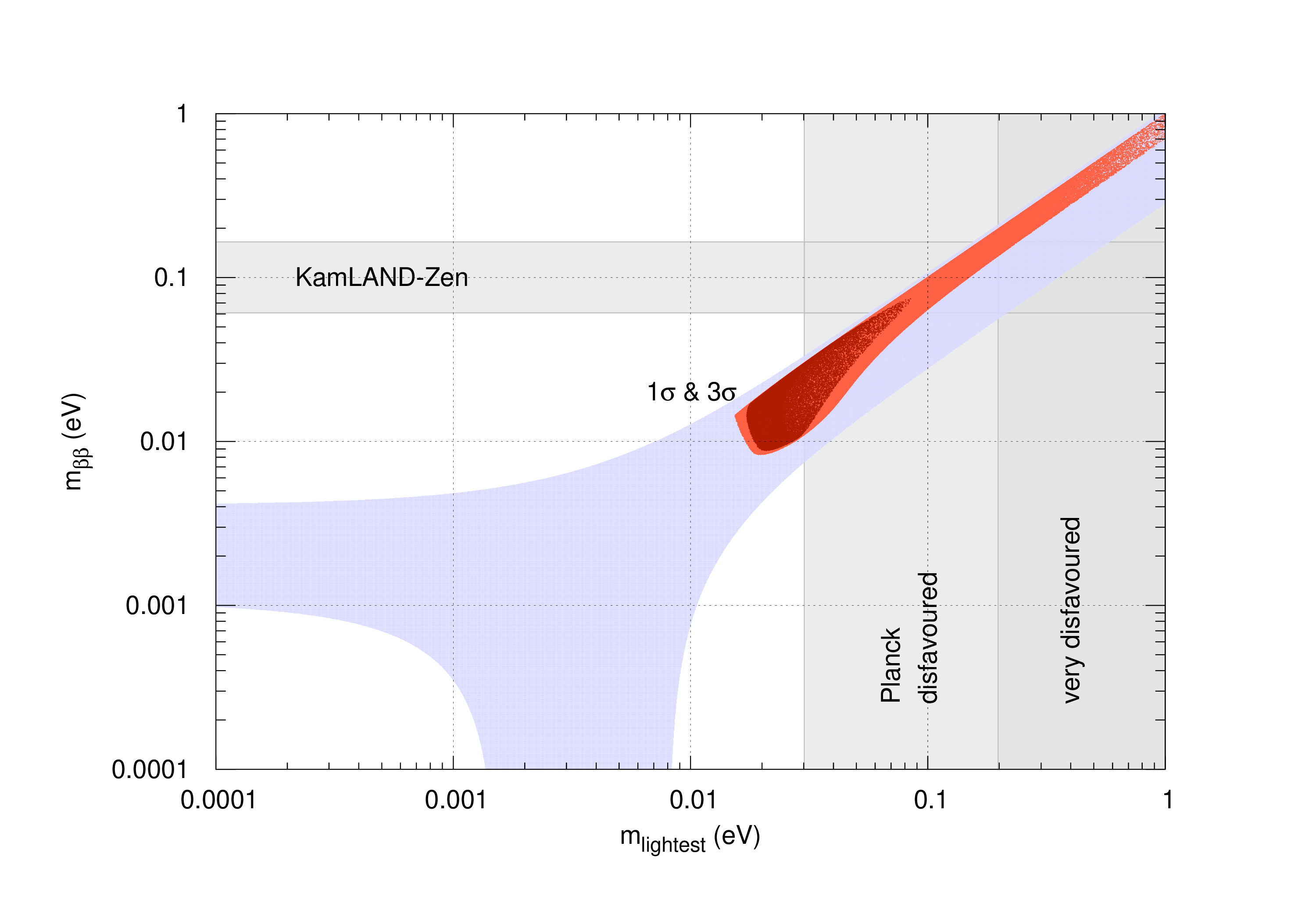
(a) Normal Ordering

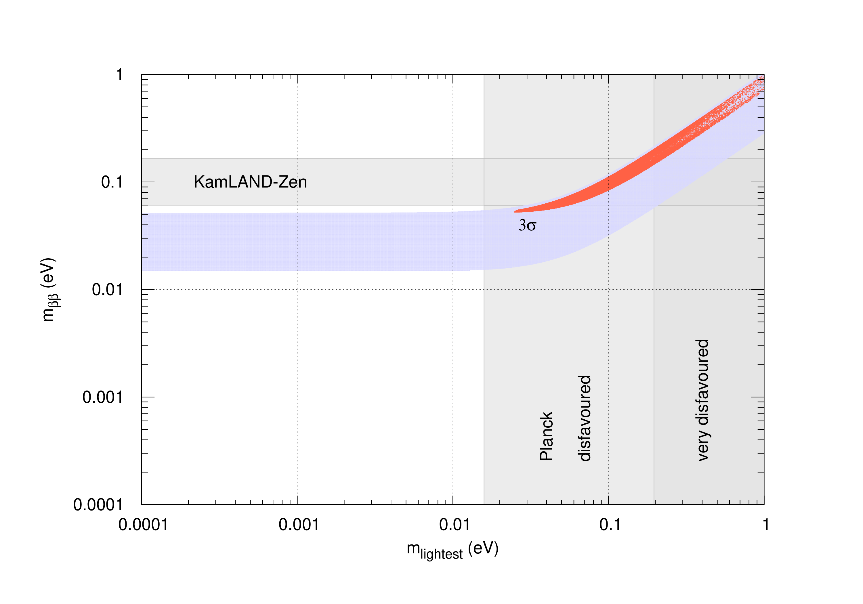
(b) Inverted Ordering

Figure 1: Predictions of $m_{\text{lightest}}$ vs $m_{\beta\beta}$ for both ordering of neutrino masses compatible with $1\sigma$ (dark-red, NO only, except $\theta_{12}$) and $3\sigma$ data from Esteban:2020cvm . In both figures there were also included the current upper limit from KamLAND-Zen $m_{\beta\beta}<61-165$ meV KamLAND-Zen:2016pfg and cosmological constraints from PLANCK 2018 (disfavoured region 0.12 eV $<\sum m_{i}<$ 0.60 eV and very disfavoured region $\sum m_{i}>0.60$ eV) Aghanim:2018eyx . In both figures there were also included the current upper limit from KamLAND-Zen $m_{\beta\beta}<61-165$ meV KamLAND-Zen:2016pfg and cosmological constraints from PLANCK 2018 (disfavoured region 0.12 eV $<\sum m_{i}<$ 0.60 eV and very disfavoured region $\sum m_{i}>0.60$ eV) Aghanim:2018eyx .

It is also possible to obtain the expected $m_{\beta\beta}$ for neutrinoless beta decay using the formula

$$m_{\beta\beta} =|(M_{\nu})_{(1,1)}|$$

$$=\left|\frac{5+\sqrt{5}}{10}m_{1}e^{-2i\alpha_{1}}\cos^{2}\theta+\frac{2m_{2}e^{-2i\alpha_{3}}}{5+\sqrt{5}}+\frac{5+\sqrt{5}}{10}m_{3}e^{2i\alpha_{2}}\sin^{2}\theta\right|,$$ (97)

where $m_{2}$ is given by Eq.(95). Doing a numerical computation, the allowed regions of $m_{\text{lightest}}$ vs $m_{\beta\beta}$ of FIG.1 (for NO, $m_{\text{lightest}}=m_{1}$ and for IO, $m_{\text{lightest}}=m_{3}$) were obtained, using again as constraints the data from Esteban:2020cvm . In both figures it is also shown the current upper limit provided by KamLAND-Zen, $m_{\beta\beta}<61-165$ meV KamLAND-Zen:2016pfg . Results from PLANCK 2018 also constrain the sum of neutrino masses, although different constrains can be obtained depending on the data considered (for more details, see Aghanim:2018eyx ). In the figures are plotted two shadowed regions, a very disfavoured region $\sum m_{i}>0.60$ eV (considering the limit 95%C.L.,Planck lensing$+$BAO$+\theta_{MC}$) and a disfavoured region $\sum m_{i}>0.12$ eV (considering the limit 95%C.L.,Planck TT,TE,EE$+$lowE$+$lensing$+$BAO$+\theta_{MC}$). These constraints on $\sum m_{i}$ can be expressed as constraints on $m_{\text{lightest}}$ using the best fit value for the squared mass differences: $m_{\text{lightest}}>0.198$ eV and $m_{\text{lightest}}>0.030$ eV for NO and $m_{\text{lightest}}>0.196$ eV and $m_{\text{lightest}}>0.016$ eV for IO, for the very disfavoured and the disfavoured regions respectively. We conclude then that both fits in TABLE 4 are in the disfavoured region.

For NO, the points that were compatible with the $1\sigma$ regions for the observables other than $\theta_{12}$ were plotted with a darker red colour. Only for normal mass orderings do we have points outside the disfavoured region. The minimum values considering the $3\sigma$ ranges are

$$(m_{\text{lightest}})_{\text{min}}^{\text{NO}}\approx 0.015\text{ eV}~{}~{} ~{}~{}(m_{\beta\beta})_{\text{min}}^{\text{NO}}\approx 0.008\text{ eV}$$

$$(m_{\text{lightest}})_{\text{min}}^{\text{IO}}\approx 0.025\text{ eV}~{}~{} ~{}~{}(m_{\beta\beta})_{\text{min}}^{\text{IO}}\approx 0.052\text{ eV},$$ (98)

and the minimum and maximum values for the points in dark-red are

$$(m_{\text{lightest}})_{\text{min}}^{\text{NO}}\approx 0.017\text{ eV}~{}~{} ~{}~{}(m_{\beta\beta})_{\text{min}}^{\text{NO}}\approx 0.009\text{ eV}$$

$$(m_{\text{lightest}})_{\text{max}}^{\text{NO}}\approx 0.085\text{ eV}~{}~{} ~{}~{}(m_{\beta\beta})_{\text{max}}^{\text{NO}}\approx 0.074\text{ eV}.$$ (99)

Taking these considerations into account, we conclude that NO is the preferred mass ordering.

VI Conclusion

In this paper we make use of the framework of multiple modular symmetries and build a model with the viable Golden Ratio 2 mixing. Relying on a minimal field content, we describe how to break the multiple $A_{5}$ to a single modular symmetry. We present choices of representations and weights for the fields that produce the model, which leads to leptonic mixing matrix that fits well with the observed values of the angles in a predictive manner. We predict neutrinoless double beta decay. Inverted ordering is disfavoured by cosmological observations and is also disfavoured by the fits to the experimental leptonic mixing observables, with the normal ordering leading to a better fit to the experimental observables.

Appendix A $A_{5}$ multiplication rules

The group $A_{5}$ is the group of even permutations of five objects and is the symmetry group of the icosahedron and its dual solid the dodecahedron. It has 60 elements and two generators, S and T:

$$S^{2}=(ST)^{3}=T^{5}=1.$$ (100)

$A_{5}$ has five conjugacy classes:

$$C_{1} =\{e\}$$ (101)

$$C_{2} =\{T^{3}ST^{2}ST,ST^{2}ST^{3},ST^{2}ST^{2}ST,ST^{3}ST,T^{3}ST^{3},T^{2}ST^{2},TS,TSTS,ST^{3}STS,T^{2}ST^{2}ST,$$

$$\hskip 42.67912ptSTST^{3},T^{3}ST,ST^{3}ST^{2},T^{3}ST^{2}S,T^{3}STS,TST^{3},ST,STST,TST^{3}ST,ST^{2}ST^{2}S\}$$ (102)

$$C_{3} =\{STST^{2},T^{2}ST^{3}STS,ST^{3}ST^{2}S,T^{2}ST^{3},S,ST^{3}ST^{2}ST,ST^{2}ST^{3}ST,T^{2}ST^{3}ST^{2},$$

$$\hskip 42.67912ptSTST^{3}ST^{2},TST^{2}S,ST^{2}ST^{3}ST^{2},ST^{2}ST,T^{3}ST^{2},T^{2}STS,TST^{3}ST^{2}S\}$$ (103)

$$C_{4} =\{T,T^{4},TST,STS,STST^{2}S,TST^{2},T^{3}S,ST^{2},T^{2}S,ST^{3},ST^{2}STS,T^{2}ST\}$$ (104)

$$C_{5} =\{T^{2},T^{3},ST^{2}S,TST^{2}ST,STST^{3}ST^{2}S,TST^{3}ST^{2},STST^{3}ST,$$

$$\hskip 42.67912ptST^{2}ST^{2},T^{2}ST^{2}S,TST^{3}STS,T^{2}ST^{3}ST,ST^{2}ST^{3}STS\}$$ (105)

This group has five irreducible representations: an invariant singlet $\mathbf{1}$, two triplets $\mathbf{3}$ and $\mathbf{3^{\prime}}$, a quadruplet $\mathbf{4}$ and a quintuplet $\mathbf{5}$. The representations for the generators are in TABLE 5.

	$S$	$T$
$\mathbf{1}$	1	1
$\mathbf{3}$	$\frac{1}{\sqrt{5}}\begin{pmatrix}1&-\sqrt{2}&-\sqrt{2}\\ -\sqrt{2}&-\phi&1/\phi\\ -\sqrt{2}&1/\phi&-\phi\end{pmatrix}$	$\begin{pmatrix}1&0&0\\ 0&\zeta&0\\ 0&0&\zeta^{4}\end{pmatrix}$
$\mathbf{3^{\prime}}$	$\frac{1}{\sqrt{5}}\begin{pmatrix}-1&\sqrt{2}&\sqrt{2}\\ \sqrt{2}&-1/\phi&\phi\\ \sqrt{2}&\phi&-1/\phi\end{pmatrix}$	$\begin{pmatrix}1&0&0\\ 0&\zeta^{2}&0\\ 0&0&\zeta^{3}\end{pmatrix}$
$\mathbf{4}$	$\frac{1}{\sqrt{5}}\begin{pmatrix}1&1/\phi&\phi&-1\\ 1/\phi&-1&1&\phi\\ \phi&1&-1&1/\phi\\ -1&\phi&1/\phi&1\end{pmatrix}$	$\begin{pmatrix}\zeta&0&0&0\\ 0&\zeta^{2}&0&0\\ 0&0&\zeta^{3}&0\\ 0&0&0&\zeta^{4}\\ \end{pmatrix}$
$\mathbf{5}$	$\frac{1}{\sqrt{5}}\begin{pmatrix}-1&\sqrt{6}&\sqrt{6}&\sqrt{6}&\sqrt{6}\\ \sqrt{6}&1/\phi^{2}&-2\phi&2/\phi&\phi^{2}\\ \sqrt{6}&-2\phi&\phi^{2}&1/\phi^{2}&2/\phi\\ \sqrt{6}&2/\phi&1/\phi^{2}&\phi^{2}&2\phi\\ \sqrt{6}&\phi^{2}&2/\phi&-2\phi&1/\phi^{2}\end{pmatrix}$	$\begin{pmatrix}1&0&0&0&0\\ 0&\zeta&0&0&0\\ 0&0&\zeta^{2}&0&0\\ 0&0&0&\zeta^{3}&0\\ 0&0&0&0&\zeta^{4}\\ \end{pmatrix}$

Table 5: Representation for the two generators of $A_{5}$, where $\phi=\frac{1+\sqrt{5}}{2}$ and $\zeta=e^{2\pi i/5}$.

The product of two irreps decomposes in the following way:

$$\mathbf{3}\otimes\mathbf{3}=\mathbf{1}\oplus\mathbf{3}\oplus\mathbf{5}$$ (106)

$$\mathbf{3}\otimes\mathbf{3^{\prime}}=\mathbf{4}\oplus\mathbf{5}$$ (107)

$$\mathbf{3}\otimes\mathbf{4}=\mathbf{3^{\prime}}\oplus\mathbf{4}\oplus\mathbf{5}$$ (108)

$$\mathbf{3}\otimes\mathbf{5}=\mathbf{3}\oplus\mathbf{3^{\prime}}\oplus\mathbf{4}\oplus\mathbf{5}$$ (109)

$$\mathbf{3^{\prime}}\otimes\mathbf{3^{\prime}}=\mathbf{1}\oplus\mathbf{3^{\prime}}\oplus\mathbf{5}$$ (110)

$$\mathbf{3^{\prime}}\otimes\mathbf{4}=\mathbf{3}\oplus\mathbf{4}\oplus\mathbf{5}$$ (111)

$$\mathbf{3^{\prime}}\otimes\mathbf{5}=\mathbf{3}\oplus\mathbf{3^{\prime}}\oplus\mathbf{4}\oplus\mathbf{5}$$ (112)

$$\mathbf{4}\otimes\mathbf{4}=\mathbf{1}\oplus\mathbf{3}\oplus\mathbf{3^{\prime}}\oplus\mathbf{4}\oplus\mathbf{5}$$ (113)

$$\mathbf{4}\otimes\mathbf{5}=\mathbf{3}\oplus\mathbf{3^{\prime}}\oplus\mathbf{4}\oplus\mathbf{5}_{1}\oplus\mathbf{5}_{2}$$ (114)

$$\mathbf{5}\otimes\mathbf{5}=\mathbf{1}\oplus\mathbf{3}\oplus\mathbf{3^{\prime}}\oplus\mathbf{4}_{1}\oplus\mathbf{4}_{2}\oplus\mathbf{5}_{1}\oplus\mathbf{5}_{2}$$ (115)

The factors considered for the representation in TABLE 5 lead to the following decomposition, with the Clebsch-Gordan coefficients in Novichkov:2018nkm :

$$\begin{pmatrix}a_{1}\\ a_{2}\\ a_{3}\end{pmatrix}_{\mathbf{3}}\otimes\begin{pmatrix}b_{1}\\ b_{2}\\ b_{3}\end{pmatrix}_{\mathbf{3}} =(a_{1}b_{1}+a_{2}b_{3}+a_{3}b_{2})_{\mathbf{1}}\oplus\begin{pmatrix}a_{2}b_{3}-a_{3}b_{2}\\ a_{1}b_{2}-a_{2}b_{1}\\ a_{3}b_{1}-a_{1}b_{3}\end{pmatrix}_{\mathbf{3}}\oplus\begin{pmatrix}2a_{1}b_{1}-a_{2}b_{3}-a_{3}b_{2}\\ -\sqrt{3}a_{1}b_{2}-\sqrt{3}a_{2}b_{1}\\ \sqrt{6}a_{2}b_{2}\\ \sqrt{6}a_{3}b_{3}\\ -\sqrt{3}a_{1}b_{3}-\sqrt{3}a_{3}b_{1}\end{pmatrix}_{\mathbf{5}}$$ (116)

$$\begin{pmatrix}a_{1}\\ a_{2}\\ a_{3}\end{pmatrix}_{\mathbf{3^{\prime}}}\otimes\begin{pmatrix}b_{1}\\ b_{2}\\ b_{3}\end{pmatrix}_{\mathbf{3^{\prime}}} =(a_{1}b_{1}+a_{2}b_{3}+a_{3}b_{2})_{\mathbf{1}}\oplus\begin{pmatrix}a_{2}b_{3}-a_{3}b_{2}\\ a_{1}b_{2}-a_{2}b_{1}\\ a_{3}b_{1}-a_{1}b_{3}\end{pmatrix}_{\mathbf{3^{\prime}}}\oplus\begin{pmatrix}2a_{1}b_{1}-a_{2}b_{3}-a_{3}b_{2}\\ \sqrt{6}a_{3}b_{3}\\ -\sqrt{3}a_{1}b_{2}-\sqrt{3}a_{2}b_{1}\\ -\sqrt{3}a_{1}b_{3}-\sqrt{3}a_{3}b_{1}\\ \sqrt{6}a_{2}b_{2}\end{pmatrix}_{\mathbf{5}}$$ (117)

$$\begin{pmatrix}a_{1}\\ a_{2}\\ a_{3}\end{pmatrix}_{\mathbf{3}}\otimes\begin{pmatrix}b_{1}\\ b_{2}\\ b_{3}\end{pmatrix}_{\mathbf{3^{\prime}}} =\begin{pmatrix}\sqrt{2}a_{2}b_{1}+a_{3}b_{2}\\ -\sqrt{2}a_{1}b_{2}-a_{3}b_{3}\\ -\sqrt{2}a_{1}b_{3}-a_{2}b_{2}\\ \sqrt{2}a_{3}b_{1}+a_{2}b_{3}\end{pmatrix}_{\mathbf{4}}\oplus\begin{pmatrix}\sqrt{3}a_{1}b_{1}\\ a_{2}b_{1}+\sqrt{2}a_{3}b_{2}\\ a_{1}b_{2}-\sqrt{2}a_{3}b_{3}\\ a_{1}b_{3}-\sqrt{2}a_{2}b_{2}\\ a_{3}b_{1}+\sqrt{2}a_{2}b_{3}\end{pmatrix}_{\mathbf{5}}$$ (118)

$$\begin{pmatrix}a_{1}\\ a_{2}\\ a_{3}\end{pmatrix}_{\mathbf{3}}\otimes\begin{pmatrix}b_{1}\\ b_{2}\\ b_{3}\\ b_{4}\end{pmatrix}_{\mathbf{4}} =\begin{pmatrix}-\sqrt{2}a_{2}b_{4}-\sqrt{2}a_{3}b_{1}\\ \sqrt{2}a_{1}b_{2}-a_{2}b_{1}+a_{3}b_{3}\\ \sqrt{2}a_{1}b_{3}-a_{3}b_{4}+a_{2}b_{2}\\ \end{pmatrix}_{\mathbf{3^{\prime}}}\oplus\begin{pmatrix}a_{1}b_{1}-\sqrt{2}a_{3}b_{2}\\ -a_{1}b_{2}-\sqrt{2}a_{2}b_{1}\\ a_{1}b_{3}+\sqrt{2}a_{3}b_{4}\\ -a_{1}b_{4}+\sqrt{2}a_{2}b_{3}\end{pmatrix}_{\mathbf{4}}\oplus$$

$$\oplus\begin{pmatrix}\sqrt{6}a_{2}b_{4}-\sqrt{6}a_{3}b_{1}\\ 2\sqrt{2}a_{1}b_{1}+2a_{3}b_{2}\\ -\sqrt{2}a_{1}b_{2}+a_{2}b_{1}+3a_{3}b_{3}\\ \sqrt{2}a_{1}b_{3}-a_{3}b_{4}-3a_{2}b_{2}\\ -2\sqrt{2}a_{1}b_{4}-2a_{2}b_{3}\end{pmatrix}_{\mathbf{5}}$$ (119)

$$\begin{pmatrix}a_{1}\\ a_{2}\\ a_{3}\end{pmatrix}_{\mathbf{3^{\prime}}}\otimes\begin{pmatrix}b_{1}\\ b_{2}\\ b_{3}\\ b_{4}\end{pmatrix}_{\mathbf{4}} =\begin{pmatrix}-\sqrt{2}a_{2}b_{3}-\sqrt{2}a_{3}b_{2}\\ \sqrt{2}a_{1}b_{1}+a_{2}b_{4}-a_{3}b_{3}\\ \sqrt{2}a_{1}b_{4}+a_{3}b_{1}-a_{2}b_{2}\\ \end{pmatrix}_{\mathbf{3}}\oplus\begin{pmatrix}a_{1}b_{1}+\sqrt{2}a_{3}b_{3}\\ a_{1}b_{2}-\sqrt{2}a_{3}b_{4}\\ -a_{1}b_{3}+\sqrt{2}a_{2}b_{1}\\ -a_{1}b_{4}-\sqrt{2}a_{2}b_{2}\end{pmatrix}_{\mathbf{4}}\oplus$$

$$\oplus\begin{pmatrix}\sqrt{6}a_{2}b_{3}-\sqrt{6}a_{3}b_{2}\\ \sqrt{2}a_{1}b_{1}-3a_{2}b_{4}-a_{3}b_{3}\\ 2\sqrt{2}a_{1}b_{2}+2a_{3}b_{4}\\ -2\sqrt{2}a_{1}b_{3}-2a_{2}b_{1}\\ -\sqrt{2}a_{1}b_{4}+3a_{3}b_{1}+a_{2}b_{2}\end{pmatrix}_{\mathbf{5}}$$ (120)

$$\begin{pmatrix}a_{1}\\ a_{2}\\ a_{3}\end{pmatrix}_{\mathbf{3}}\otimes\begin{pmatrix}b_{1}\\ b_{2}\\ b_{3}\\ b_{4}\\ b_{5}\end{pmatrix}_{\mathbf{5}} =\begin{pmatrix}-2a_{1}b_{1}+\sqrt{3}a_{2}b_{5}+\sqrt{3}a_{3}b_{2}\\ \sqrt{3}a_{1}b_{2}+a_{2}b_{1}-\sqrt{6}a_{3}b_{3}\\ \sqrt{3}a_{1}b_{5}+a_{3}b_{1}-\sqrt{6}a_{2}b_{4}\\ \end{pmatrix}_{\mathbf{3}}\oplus\begin{pmatrix}\sqrt{3}a_{1}b_{1}+a_{2}b_{5}+a_{3}b_{2}\\ a_{1}b_{3}-\sqrt{2}a_{2}b_{2}-\sqrt{2}a_{3}b_{4}\\ a_{1}b_{4}-\sqrt{2}a_{2}b_{3}-\sqrt{2}a_{3}b_{5}\\ \end{pmatrix}_{\mathbf{3^{\prime}}}\oplus$$

$$\oplus\begin{pmatrix}2\sqrt{2}a_{1}b_{2}-\sqrt{6}a_{2}b_{1}+a_{3}b_{3}\\ -\sqrt{2}a_{1}b_{3}+2a_{2}b_{2}-3a_{3}b_{4}\\ \sqrt{2}a_{1}b_{4}-2a_{2}b_{5}+3a_{2}b_{3}\\ -2\sqrt{2}a_{1}b_{5}+\sqrt{6}a_{3}b_{1}-a_{2}b_{4}\end{pmatrix}_{\mathbf{4}}\oplus\begin{pmatrix}\sqrt{3}a_{2}b_{5}-\sqrt{3}a_{3}b_{2}\\ -a_{1}b_{2}-\sqrt{3}a_{2}b_{1}-\sqrt{2}a_{3}b_{3}\\ -2a_{1}b_{3}-\sqrt{2}a_{2}b_{2}\\ 2a_{1}b_{4}+\sqrt{2}a_{3}b_{5}\\ a_{1}b_{5}+\sqrt{3}a_{3}b_{1}+\sqrt{2}a_{2}b_{4}\end{pmatrix}_{\mathbf{5}}$$ (121)

$$\begin{pmatrix}a_{1}\\ a_{2}\\ a_{3}\end{pmatrix}_{\mathbf{3^{\prime}}}\otimes\begin{pmatrix}b_{1}\\ b_{2}\\ b_{3}\\ b_{4}\\ b_{5}\end{pmatrix}_{\mathbf{5}} =\begin{pmatrix}\sqrt{3}a_{1}b_{1}+a_{2}b_{4}+a_{3}b_{3}\\ a_{1}b_{2}-\sqrt{2}a_{2}b_{5}-\sqrt{2}a_{3}b_{4}\\ a_{1}b_{5}-\sqrt{2}a_{2}b_{3}-\sqrt{2}a_{3}b_{2}\\ \end{pmatrix}_{\mathbf{3}}\oplus\begin{pmatrix}-2a_{1}b_{1}+\sqrt{3}a_{2}b_{4}+\sqrt{3}a_{3}b_{3}\\ \sqrt{3}a_{1}b_{3}+a_{2}b_{1}-\sqrt{6}a_{3}b_{5}\\ \sqrt{3}a_{1}b_{4}+a_{3}b_{1}-\sqrt{6}a_{2}b_{2}\\ \end{pmatrix}_{\mathbf{3^{\prime}}}\oplus$$

$$\oplus\begin{pmatrix}\sqrt{2}a_{1}b_{2}-2a_{3}b_{4}+3a_{2}b_{5}\\ 2\sqrt{2}a_{1}b_{3}-\sqrt{6}a_{2}b_{1}+a_{3}b_{5}\\ -2\sqrt{2}a_{1}b_{4}+\sqrt{6}a_{3}b_{1}-a_{2}b_{2}\\ -\sqrt{2}a_{1}b_{5}+2a_{2}b_{3}-3a_{3}b_{2}\end{pmatrix}_{\mathbf{4}}\oplus\begin{pmatrix}\sqrt{3}a_{2}b_{4}-\sqrt{3}a_{3}b_{3}\\ 2a_{1}b_{2}+\sqrt{2}a_{3}b_{4}\\ -a_{1}b_{3}-\sqrt{3}a_{2}b_{1}-\sqrt{2}a_{3}b_{5}\\ a_{1}b_{4}+\sqrt{3}a_{3}b_{1}+\sqrt{2}a_{2}b_{2}\\ -2a_{1}b_{5}-\sqrt{2}a_{2}b_{3}\end{pmatrix}_{\mathbf{5}}$$ (122)

$$\begin{pmatrix}a_{1}\\ a_{2}\\ a_{3}\\ a_{4}\end{pmatrix}_{\mathbf{4}}\otimes\begin{pmatrix}b_{1}\\ b_{2}\\ b_{3}\\ b_{4}\end{pmatrix}_{\mathbf{4}} =(a_{1}b_{4}+a_{2}b_{3}+a_{3}b_{2}+a_{4}b_{1})_{\mathbf{1}}\oplus\begin{pmatrix}a_{2}b_{3}-a_{3}b_{2}+a_{4}b_{1}-a_{1}b_{4}\\ \sqrt{2}a_{2}b_{4}-\sqrt{2}a_{4}b_{2}\\ \sqrt{2}a_{1}b_{3}-\sqrt{2}a_{3}b_{1}\end{pmatrix}_{\mathbf{3}}\oplus$$

$$\oplus\begin{pmatrix}a_{2}b_{3}-a_{3}b_{2}+a_{1}b_{4}-a_{4}b_{1}\\ \sqrt{2}a_{3}b_{4}-\sqrt{2}a_{4}b_{3}\\ \sqrt{2}a_{1}b_{2}-\sqrt{2}a_{2}b_{1}\end{pmatrix}_{\mathbf{3}}\oplus\begin{pmatrix}a_{3}b_{3}+a_{2}b_{4}+a_{4}b_{2}\\ a_{1}b_{1}+a_{3}b_{4}+a_{4}b_{3}\\ a_{4}b_{4}+a_{1}b_{2}+a_{2}b_{1}\\ a_{2}b_{2}+a_{1}b_{3}+a_{3}b_{1}\\ \end{pmatrix}_{\mathbf{4}}\oplus$$

$$\oplus\begin{pmatrix}\sqrt{3}a_{1}b_{4}+\sqrt{3}a_{4}b_{1}-\sqrt{3}a_{2}b_{3}-\sqrt{3}a_{3}b_{2}\\ 2\sqrt{2}a_{3}b_{3}-\sqrt{2}a_{2}b_{4}-\sqrt{2}a_{4}b_{2}\\ -2\sqrt{2}a_{1}b_{1}+\sqrt{2}a_{3}b_{4}+\sqrt{2}a_{4}b_{3}\\ -2\sqrt{2}a_{4}b_{4}+\sqrt{2}a_{1}b_{2}-\sqrt{2}a_{2}b_{1}\\ 2\sqrt{2}a_{2}b_{2}-\sqrt{2}a_{1}b_{3}-\sqrt{2}a_{3}b_{1}\end{pmatrix}_{\mathbf{5}}$$ (123)

$$\begin{pmatrix}a_{1}\\ a_{2}\\ a_{3}\\ a_{4}\end{pmatrix}_{\mathbf{4}}\otimes\begin{pmatrix}b_{1}\\ b_{2}\\ b_{3}\\ b_{4}\\ b_{5}\end{pmatrix}_{\mathbf{5}} =\begin{pmatrix}2\sqrt{2}a_{1}b_{5}-2\sqrt{2}a_{4}b_{2}+\sqrt{2}a_{3}b_{3}-\sqrt{2}a_{2}b_{4}\\ 3a_{3}b_{4}+2a_{2}b_{5}-a_{4}b_{3}-\sqrt{6}a_{1}b_{1}\\ -3a_{2}b_{3}-2a_{3}b_{2}+a_{1}b_{4}+\sqrt{6}a_{4}b_{1}\end{pmatrix}_{\mathbf{3}}\oplus$$

$$\oplus\begin{pmatrix}2\sqrt{2}a_{2}b_{4}-2\sqrt{2}a_{3}b_{3}+\sqrt{2}a_{1}b_{5}-\sqrt{2}a_{4}b_{2}\\ 3a_{1}b_{2}+2a_{4}b_{4}-a_{3}b_{5}-\sqrt{6}a_{2}b_{1}\\ -3a_{4}b_{5}-2a_{1}b_{3}+a_{2}b_{2}+\sqrt{6}a_{3}b_{1}\end{pmatrix}_{\mathbf{3^{\prime}}}\oplus$$

$$\oplus\begin{pmatrix}\sqrt{3}a_{1}b_{1}-\sqrt{2}a_{2}b_{5}+\sqrt{2}a_{3}b_{4}-2\sqrt{2}a_{4}b_{3}\\ -\sqrt{2}a_{1}b_{2}-\sqrt{3}a_{2}b_{1}+2\sqrt{2}a_{3}b_{5}+\sqrt{2}a_{4}b_{4}\\ \sqrt{2}a_{1}b_{3}+2\sqrt{2}a_{2}b_{2}-\sqrt{3}a_{3}b_{1}-\sqrt{2}a_{4}b_{5}\\ -2\sqrt{2}a_{1}b_{4}+\sqrt{2}a_{2}b_{3}-\sqrt{2}a_{3}b_{2}+\sqrt{3}a_{4}b_{1}\end{pmatrix}_{\mathbf{4}}\oplus$$

$$\oplus\begin{pmatrix}\sqrt{2}a_{1}b_{5}-\sqrt{2}a_{2}b_{4}-\sqrt{2}a_{3}b_{3}+\sqrt{2}a_{4}b_{2}\\ -\sqrt{2}a_{1}b_{1}-\sqrt{3}a_{3}b_{4}-\sqrt{3}a_{4}b_{3}\\ \sqrt{3}a_{1}b_{2}+\sqrt{2}a_{2}b_{1}+\sqrt{3}a_{3}b_{5}\\ \sqrt{3}a_{2}b_{2}+\sqrt{2}a_{3}b_{1}+\sqrt{3}a_{4}b_{5}\\ -\sqrt{3}a_{1}b_{4}-\sqrt{3}a_{2}b_{3}-\sqrt{2}a_{4}b_{1}\end{pmatrix}_{\mathbf{5}_{1}}\oplus$$

$$\oplus\begin{pmatrix}2a_{1}b_{5}+4a_{2}b_{4}+4a_{3}b_{3}+2a_{4}b_{2}\\ 4a_{1}b_{1}+2\sqrt{6}a_{2}b_{5}\\ -\sqrt{6}a_{1}b_{2}+2a_{2}b_{1}-\sqrt{6}a_{3}b_{5}+2\sqrt{6}a_{4}b_{4}\\ 2\sqrt{6}a_{1}b_{3}-\sqrt{6}a_{2}b_{2}+2a_{3}b_{1}-\sqrt{6}a_{4}b_{5}\\ 2\sqrt{6}a_{3}b_{2}+4a_{4}b_{1}\end{pmatrix}_{\mathbf{5}_{2}}$$ (124)

$$\begin{pmatrix}a_{1}\\ a_{2}\\ a_{3}\\ a_{4}\\ a_{5}\end{pmatrix}_{\mathbf{5}}\otimes\begin{pmatrix}b_{1}\\ b_{2}\\ b_{3}\\ b_{4}\\ b_{5}\end{pmatrix}_{\mathbf{5}} =(a_{1}b_{1}+a_{2}b_{5}+a_{5}b_{2}+a_{3}b_{4}+a_{4}b_{3})_{\mathbf{1}}\oplus$$

$$\oplus\begin{pmatrix}a_{2}b_{5}-a_{5}b_{2}+2a_{3}b_{4}-2a_{4}b_{3}\\ \sqrt{3}a_{2}b_{1}-\sqrt{3}a_{1}b_{2}+\sqrt{2}a_{3}b_{5}-\sqrt{2}a_{5}b_{3}\\ \sqrt{3}a_{1}b_{5}-\sqrt{3}a_{5}b_{1}+\sqrt{2}a_{2}b_{4}-\sqrt{2}a_{2}b_{4}\end{pmatrix}_{\mathbf{3}}\oplus$$

$$\oplus\begin{pmatrix}a_{4}b_{3}-a_{3}b_{4}+2a_{2}b_{5}-2a_{5}b_{2}\\ \sqrt{3}a_{1}b_{3}-\sqrt{3}a_{3}b_{1}+\sqrt{2}a_{4}b_{5}-\sqrt{2}a_{5}b_{4}\\ \sqrt{3}a_{4}b_{1}-\sqrt{3}a_{1}b_{4}+\sqrt{2}a_{2}b_{3}-\sqrt{2}a_{3}b_{4}\end{pmatrix}_{\mathbf{3^{\prime}}}\oplus$$

$$\oplus\begin{pmatrix}4\sqrt{3}a_{4}b_{4}+3\sqrt{2}a_{1}b_{2}+3\sqrt{2}a_{2}b_{1}-\sqrt{3}a_{3}b_{5}-\sqrt{3}a_{5}b_{3}\\ 4\sqrt{3}a_{2}b_{2}+3\sqrt{2}a_{1}b_{3}+3\sqrt{2}a_{3}b_{1}-\sqrt{3}a_{4}b_{5}-\sqrt{3}a_{5}b_{4}\\ 4\sqrt{3}a_{5}b_{5}+3\sqrt{2}a_{1}b_{4}+3\sqrt{2}a_{4}b_{1}-\sqrt{3}a_{3}b_{2}-\sqrt{3}a_{2}b_{3}\\ 4\sqrt{3}a_{3}b_{3}+3\sqrt{2}a_{1}b_{5}+3\sqrt{2}a_{5}b_{1}-\sqrt{3}a_{2}b_{4}-\sqrt{3}a_{4}b_{2}\end{pmatrix}_{\mathbf{4}_{1}}\oplus$$

$$\oplus\begin{pmatrix}\sqrt{2}a_{1}b_{2}-\sqrt{2}a_{2}b_{1}+\sqrt{3}a_{3}b_{5}-\sqrt{3}a_{5}b_{3}\\ \sqrt{2}a_{3}b_{1}-\sqrt{2}a_{1}b_{3}+\sqrt{3}a_{4}b_{5}-\sqrt{3}a_{5}b_{4}\\ \sqrt{2}a_{4}b_{1}-\sqrt{2}a_{1}b_{4}+\sqrt{3}a_{3}b_{2}-\sqrt{3}a_{2}b_{3}\\ \sqrt{2}a_{1}b_{5}-\sqrt{2}a_{5}b_{1}+\sqrt{3}a_{4}b_{2}-\sqrt{3}a_{2}b_{4}\end{pmatrix}_{\mathbf{4}_{2}}\oplus$$

$$\oplus\begin{pmatrix}2a_{1}b_{1}+a_{2}b_{5}+a_{5}b_{2}-2a_{3}b_{4}-2a_{4}b_{3}\\ a_{1}b_{2}+a_{2}b_{1}+\sqrt{6}a_{3}b_{5}+\sqrt{6}a_{5}b_{3}\\ \sqrt{6}a_{2}b_{2}-2a_{1}b_{3}-2a_{3}b_{1}\\ \sqrt{6}a_{5}b_{5}-2a_{1}b_{4}-2a_{4}b_{1}\\ a_{1}b_{5}+a_{5}b_{1}+\sqrt{6}a_{2}b_{4}+\sqrt{6}a_{4}b_{2}\end{pmatrix}_{\mathbf{5}_{1}}\oplus$$

$$\oplus\begin{pmatrix}2a_{1}b_{1}+a_{3}b_{4}+a_{4}b_{3}-2a_{2}b_{5}-2a_{5}b_{2}\\ \sqrt{6}a_{4}b_{4}-2a_{1}b_{2}-2a_{2}b_{1}\\ a_{1}b_{3}+a_{3}b_{1}+\sqrt{6}a_{4}b_{5}+\sqrt{6}a_{5}b_{4}\\ a_{1}b_{4}+a_{4}b_{1}+\sqrt{6}a_{2}b_{3}+\sqrt{6}a_{3}b_{2}\\ \sqrt{6}a_{3}b_{3}-2a_{1}b_{5}-2a_{5}b_{1}\end{pmatrix}_{\mathbf{5}_{2}}$$ (125)

Appendix B Modular forms of weight 2 for $A_{5}$

The linear space of modular forms of level $N=5$ and weight 2 has dimension 11. These modular functions are arranged into two triplets $\mathbf{3}$ and $\mathbf{3^{\prime}}$ and a quintuplet $\mathbf{5}$ of $\Gamma_{5}$. Modular forms of higher weight can be constructed from polynomials of these eleven modular functions.

The weight 2 modular functions can be expressed as linear combinations of logarithmic derivatives of some functions $\alpha_{i,j}(\tau)$, closed under the action of $A_{5}$, and these can be in terms of the theta function $\theta_{3}(z(\tau),t(\tau))$:

$$\theta_{3}(z,t)=\sum_{k\in\mathbb{Z}}q^{k^{2}}e^{2\pi ikz}=1+2\sum_{k\in\mathbb{N}}q^{k^{2}}\cos(2\pi kz)\,,\,q=e^{\pi it}$$ (126)

The seed functions $\alpha_{i,j}(\tau)$ are explicitly:

$$\begin{aligned} \alpha_{1,-1}(\tau)&\equiv\theta_{3}\left(\frac{\tau+1}{2},5\tau\right),\\ \alpha_{1,0}(\tau)&\equiv\theta_{3}\left(\frac{\tau+9}{10},\frac{\tau}{5}\right),\\ \alpha_{1,1}(\tau)&\equiv\theta_{3}\left(\frac{\tau}{10},\frac{\tau+1}{5}\right),\\ \alpha_{1,2}(\tau)&\equiv\theta_{3}\left(\frac{\tau+1}{10},\frac{\tau+2}{5}\right),\\ \alpha_{1,3}(\tau)&\equiv\theta_{3}\left(\frac{\tau+2}{10},\frac{\tau+3}{5}\right),\\ \alpha_{1,4}(\tau)&\equiv\theta_{3}\left(\frac{\tau+3}{10},\frac{\tau+4}{5}\right),\end{aligned}\qquad\begin{aligned} \alpha_{2,-1}(\tau)&\equiv e^{2\pi i\tau/5}\theta_{3}\left(\frac{3\tau+1}{2},5\tau\right),\\ \alpha_{2,0}(\tau)&\equiv\theta_{3}\left(\frac{\tau+7}{10},\frac{\tau}{5}\right),\\ \alpha_{2,1}(\tau)&\equiv\theta_{3}\left(\frac{\tau+8}{10},\frac{\tau+1}{5}\right),\\ \alpha_{2,2}(\tau)&\equiv\theta_{3}\left(\frac{\tau+9}{10},\frac{\tau+2}{5}\right),\\ \alpha_{2,3}(\tau)&\equiv\theta_{3}\left(\frac{\tau}{10},\frac{\tau+3}{5}\right),\\ \alpha_{2,4}(\tau)&\equiv\theta_{3}\left(\frac{\tau+1}{10},\frac{\tau+4}{5}\right).\end{aligned}$$ (127)

The linear combination of the logarithmic derivatives of these functions,

$$Y(c_{1,-1},\ldots,c_{1,4};c_{2,-1},\ldots,c_{2,4}|\tau)\equiv\sum_{i,j}c_{i,j}\frac{{\rm d}}{{\rm d}\tau}\log\alpha_{i,j}(\tau),\quad\textrm{with }\sum_{i,j}c_{i,j}=0,$$ (128)

span the linear space of the modular forms of level $N=5$ and weight 2. These are then divided into the multiplets:

$$Y_{\mathbf{5}}(\tau)=\begin{pmatrix}Y_{1}(\tau)\\ Y_{2}(\tau)\\ Y_{3}(\tau)\\ Y_{4}(\tau)\\ Y_{5}(\tau)\end{pmatrix} \equiv\begin{pmatrix}-\frac{1}{\sqrt{6}}Y\left(-5,1,1,1,1,1;-5,1,1,1,1,1\middle|\tau\right)\\ Y(0,1,\zeta^{4},\zeta^{3},\zeta^{2},\zeta;0,1,\zeta^{4},\zeta^{3},\zeta^{2},\zeta|\tau)\\ Y(0,1,\zeta^{3},\zeta,\zeta^{4},\zeta^{2};0,1,\zeta^{3},\zeta,\zeta^{4},\zeta^{2}|\tau)\\ Y(0,1,\zeta^{2},\zeta^{4},\zeta,\zeta^{3};0,1,\zeta^{2},\zeta^{4},\zeta,\zeta^{3}|\tau)\\ Y(0,1,\zeta,\zeta^{2},\zeta^{3},\zeta^{4};0,1,\zeta,\zeta^{2},\zeta^{3},\zeta^{4}|\tau)\end{pmatrix},$$ (129)

$$Y_{\mathbf{3}}(\tau)=\begin{pmatrix}Y_{6}(\tau)\\ Y_{7}(\tau)\\ Y_{8}(\tau)\end{pmatrix} \equiv\begin{pmatrix}\frac{1}{\sqrt{2}}Y\left(-\sqrt{5},-1,-1,-1,-1,-1;\sqrt{5},1,1,1,1,1\middle|\tau\right)\\ Y(0,1,\zeta^{4},\zeta^{3},\zeta^{2},\zeta;0,-1,-\zeta^{4},-\zeta^{3},-\zeta^{2},-\zeta|\tau)\\ Y(0,1,\zeta,\zeta^{2},\zeta^{3},\zeta^{4};0,-1,-\zeta,-\zeta^{2},-\zeta^{3},-\zeta^{4}|\tau)\end{pmatrix},$$ (130)

$$Y_{\mathbf{3^{\prime}}}(\tau)=\begin{pmatrix}Y_{9}(\tau)\\ Y_{10}(\tau)\\ Y_{11}(\tau)\end{pmatrix} \equiv\begin{pmatrix}\frac{1}{\sqrt{2}}Y\left(\sqrt{5},-1,-1,-1,-1,-1;-\sqrt{5},1,1,1,1,1\middle|\tau\right)\\ Y(0,1,\zeta^{3},\zeta,\zeta^{4},\zeta^{2};0,-1,-\zeta^{3},-\zeta,-\zeta^{4},-\zeta^{2}|\tau)\\ Y(0,1,\zeta^{2},\zeta^{4},\zeta,\zeta^{3};0,-1,-\zeta^{2},-\zeta^{4},-\zeta,-\zeta^{3}|\tau)\end{pmatrix},$$ (131)

where $\zeta=e^{2\pi i/5}$.

Appendix C Vacuum alignments for bi-quintuplet $\Phi$ in $A_{5}$

In this Appendix we consider how to align the VEV of the bi-quintuplet $\Phi$. Following from deMedeirosVarzielas:2019cyj and deMedeirosVarzielas:2021pug where an alignment was obtained in the context of $S_{4}$ and $A_{4}$ respectively, we add two driving fields, with the properties present in TABLE 6.

Fields	$A_{5}^{l}$	$A_{5}^{\nu}$	$2k_{l}$	$2k_{\nu}$
$\chi_{l\nu}$	$\mathbf{5}$	$\mathbf{5}$	0	0
$\chi_{l}$	$\mathbf{5}$	$\mathbf{1}$	0	0

Table 6: Transformation properties of the fields responsible for the vacuum alignment of the bi-quintuplet $\Phi$.

The superpotential responsible for the vacuum alignment that will be minimised with relation to the driving fields is

$$w=\Phi\Phi\chi_{l\nu}+M\Phi\chi_{l\nu}+\Phi\Phi\chi_{l}.$$ (132)

With this field content, we are only interested in contractions of quintuplets to give quintuplets or singlets. Minimising this superpotential in order to the driving fields leads us to the constraints:

$$\sum_{j,k=1,\ldots,5}~{}\sum_{\beta,\gamma=1,\ldots,5}\Big{(}h_{11}P^{(\mathbf{5}\otimes\mathbf{5})_{\mathbf{5}_{1}}}_{ijk}P^{(\mathbf{5}\otimes\mathbf{5})_{\mathbf{5}_{1}}}_{\alpha\beta\gamma}+h_{21}P^{(\mathbf{5}\otimes\mathbf{5})_{\mathbf{5}_{2}}}_{ijk}P^{(\mathbf{5}\otimes\mathbf{5})_{\mathbf{5}_{1}}}_{\alpha\beta\gamma}+$$

$$\hskip 99.58464pt+h_{12}P^{(\mathbf{5}\otimes\mathbf{5})_{\mathbf{5}_{1}}}_{ijk}P^{(\mathbf{5}\otimes\mathbf{5})_{\mathbf{5}_{2}}}_{\alpha\beta\gamma}+h_{22}P^{(\mathbf{5}\otimes\mathbf{5})_{\mathbf{5}_{2}}}_{ijk}P^{(\mathbf{5}\otimes\mathbf{5})_{\mathbf{5}_{2}}}_{\alpha\beta\gamma}\Big{)}(\Phi)_{j\beta}(\Phi)_{k\gamma}+M(\Phi)_{i\alpha}=0,$$ (133)

$$\hskip 28.45274pt~{}\text{for}~{}i=1,\ldots,5,\alpha=1,\ldots,5$$

$$\sum_{j,k=1,\ldots,5}~{}\sum_{\alpha,\beta=1,\ldots,5}P^{(\mathbf{5}\otimes\mathbf{5})_{\mathbf{1}}}_{\alpha\beta}\left(h_{1}P^{(\mathbf{5}\otimes\mathbf{5})_{\mathbf{5}_{1}}}_{ijk}+h_{2}P^{(\mathbf{5}\otimes\mathbf{5})_{\mathbf{5}_{2}}}_{ijk}\right)(\Phi)_{j\alpha}(\Phi)_{k\beta}=0~{}~{}\text{for}~{}~{}i=1,\ldots,5.$$ (134)

where $5\times 5$ matrices that describe the multiplication rules in Section A were introduced:

$$P^{(\mathbf{5}\otimes\mathbf{5})_{\mathbf{1}}} =\begin{pmatrix}1&0&0&0&0\\ 0&0&0&0&1\\ 0&0&0&1&0\\ 0&0&1&0&0\\ 0&1&0&0&0\\ \end{pmatrix}$$ (135)

$$P^{(\mathbf{5}\otimes\mathbf{5})_{\mathbf{5}_{1}}} =\left(\begin{pmatrix}2&0&0&0&0\\ 0&0&0&0&1\\ 0&0&0&-2&0\\ 0&0&-2&0&0\\ 0&1&0&0&0\\ \end{pmatrix},\begin{pmatrix}0&1&0&0&0\\ 1&0&0&0&0\\ 0&0&0&0&\sqrt{6}\\ 0&0&0&0&0\\ 0&0&\sqrt{6}&0&0\\ \end{pmatrix},\begin{pmatrix}0&0&-2&0&0\\ 0&\sqrt{6}&0&0&0\\ -2&0&0&0&0\\ 0&0&0&0&0\\ 0&0&0&0&0\\ \end{pmatrix},\right.$$

$$\hskip 56.9055pt\left.\begin{pmatrix}0&0&0&-2&0\\ 0&0&0&0&0\\ 0&0&0&0&0\\ -2&0&0&0&0\\ 0&0&0&0&\sqrt{6}\\ \end{pmatrix},\begin{pmatrix}0&0&0&0&1\\ 0&0&0&\sqrt{6}&0\\ 0&0&0&0&0\\ 0&\sqrt{6}&0&0&0\\ 1&0&0&0&0\\ \end{pmatrix}\right)$$ (136)

$$P^{(\mathbf{5}\otimes\mathbf{5})_{\mathbf{5}_{2}}} =\left(\begin{pmatrix}2&0&0&0&0\\ 0&0&0&0&-2\\ 0&0&0&1&0\\ 0&0&1&0&0\\ 0&-2&0&0&0\\ \end{pmatrix},\begin{pmatrix}0&-2&0&0&0\\ -2&0&0&0&0\\ 0&0&0&0&0\\ 0&0&0&\sqrt{6}&0\\ 0&0&0&0&0\\ \end{pmatrix},\begin{pmatrix}0&0&1&0&0\\ 0&0&0&0&0\\ 1&0&0&0&0\\ 0&0&0&0&\sqrt{6}\\ 0&0&0&\sqrt{6}&0\\ \end{pmatrix},\right.$$

$$\hskip 56.9055pt\left.\begin{pmatrix}0&0&0&1&0\\ 0&0&\sqrt{6}&0&0\\ 0&\sqrt{6}&0&0&0\\ 1&0&0&0&0\\ 0&0&0&0&0\\ \end{pmatrix},\begin{pmatrix}0&0&0&0&-2\\ 0&0&0&0&0\\ 0&0&\sqrt{6}&0&0\\ 0&0&0&0&0\\ -2&0&0&0&0\\ \end{pmatrix}\right)$$ (137)

The solutions of the constraints in Eq.(134) are the 60 elements of $A_{5}$ in the five dimensional representation, including the VEV that is used in the main text for $\Phi$:

$$\langle\Phi\rangle=v_{\Phi}~{}\begin{pmatrix}1&0&0&0&0\\ 0&0&0&0&1\\ 0&0&0&1&0\\ 0&0&1&0&0\\ 0&1&0&0&0\\ \end{pmatrix}=v_{\Phi}P_{\pi}.$$ (138)

References

- (1) T. Kobayashi, K. Tanaka and T. H. Tatsuishi, Phys. Rev. D 98 (2018) no.1, 016004 doi:10.1103/PhysRevD.98.016004 [arXiv:1803.10391 [hep-ph]].
- (2) T. Kobayashi, Y. Shimizu, K. Takagi, M. Tanimoto, T. H. Tatsuishi and H. Uchida, Phys. Lett. B 794 (2019), 114-121 doi:10.1016/j.physletb.2019.05.034 [arXiv:1812.11072 [hep-ph]].
- (3) H. Okada and Y. Orikasa, Phys. Rev. D 100 (2019) no.11, 115037 doi:10.1103/PhysRevD.100.115037 [arXiv:1907.04716 [hep-ph]].
- (4) S. Mishra, [arXiv:2008.02095 [hep-ph]].
- (5) X. Du and F. Wang, JHEP 02 (2021), 221 doi:10.1007/JHEP02(2021)221 [arXiv:2012.01397 [hep-ph]].
- (6) F. Feruglio, doi:10.1142/9789813238053_0012 [arXiv:1706.08749 [hep-ph]].
- (7) J. C. Criado and F. Feruglio, SciPost Phys. 5 (2018) no.5, 042 doi:10.21468/SciPostPhys.5.5.042 [arXiv:1807.01125 [hep-ph]].
- (8) T. Kobayashi, N. Omoto, Y. Shimizu, K. Takagi, M. Tanimoto and T. H. Tatsuishi, JHEP 11 (2018), 196 doi:10.1007/JHEP11(2018)196 [arXiv:1808.03012 [hep-ph]].
- (9) H. Okada and M. Tanimoto, Phys. Lett. B 791 (2019), 54-61 doi:10.1016/j.physletb.2019.02.028 [arXiv:1812.09677 [hep-ph]].
- (10) P. P. Novichkov, S. T. Petcov and M. Tanimoto, Phys. Lett. B 793 (2019), 247-258 doi:10.1016/j.physletb.2019.04.043 [arXiv:1812.11289 [hep-ph]].
- (11) T. Nomura and H. Okada, Phys. Lett. B 797 (2019), 134799 doi:10.1016/j.physletb.2019.134799 [arXiv:1904.03937 [hep-ph]].
- (12) T. Nomura and H. Okada, Nucl. Phys. B 966 (2021), 115372 doi:10.1016/j.nuclphysb.2021.115372 [arXiv:1906.03927 [hep-ph]].
- (13) G. J. Ding, S. F. King and X. G. Liu, JHEP 09 (2019), 074 doi:10.1007/JHEP09(2019)074 [arXiv:1907.11714 [hep-ph]].
- (14) D. Zhang, Nucl. Phys. B 952 (2020), 114935 doi:10.1016/j.nuclphysb.2020.114935 [arXiv:1910.07869 [hep-ph]].
- (15) H. Okada and Y. Orikasa, [arXiv:1907.13520 [hep-ph]].
- (16) T. Nomura, H. Okada and O. Popov, Phys. Lett. B 803 (2020), 135294 doi:10.1016/j.physletb.2020.135294 [arXiv:1908.07457 [hep-ph]].
- (17) T. Asaka, Y. Heo, T. H. Tatsuishi and T. Yoshida, JHEP 01 (2020), 144 doi:10.1007/JHEP01(2020)144 [arXiv:1909.06520 [hep-ph]].
- (18) T. Nomura, H. Okada and S. Patra, Nucl. Phys. B 967 (2021), 115395 doi:10.1016/j.nuclphysb.2021.115395 [arXiv:1912.00379 [hep-ph]].
- (19) T. Kobayashi, T. Nomura and T. Shimomura, Phys. Rev. D 102 (2020) no.3, 035019 doi:10.1103/PhysRevD.102.035019 [arXiv:1912.00637 [hep-ph]].
- (20) X. Wang, Nucl. Phys. B 957 (2020), 115105 doi:10.1016/j.nuclphysb.2020.115105 [arXiv:1912.13284 [hep-ph]].
- (21) H. Okada and Y. Shoji, Nucl. Phys. B 961 (2020), 115216 doi:10.1016/j.nuclphysb.2020.115216 [arXiv:2003.13219 [hep-ph]].
- (22) G. J. Ding and F. Feruglio, JHEP 06 (2020), 134 doi:10.1007/JHEP06(2020)134 [arXiv:2003.13448 [hep-ph]].
- (23) M. K. Behera, S. Mishra, S. Singirala and R. Mohanta, Phys. Dark Univ. 36 (2022), 101027 doi:10.1016/j.dark.2022.101027 [arXiv:2007.00545 [hep-ph]].
- (24) T. Nomura and H. Okada, [arXiv:2007.04801 [hep-ph]].
- (25) T. Nomura and H. Okada, [arXiv:2007.15459 [hep-ph]].
- (26) M. K. Behera, S. Singirala, S. Mishra and R. Mohanta, J. Phys. G 49 (2022) no.3, 035002 doi:10.1088/1361-6471/ac3cc2 [arXiv:2009.01806 [hep-ph]].
- (27) T. Asaka, Y. Heo and T. Yoshida, Phys. Lett. B 811 (2020), 135956 doi:10.1016/j.physletb.2020.135956 [arXiv:2009.12120 [hep-ph]].
- (28) K. I. Nagao and H. Okada, Nucl. Phys. B 980 (2022), 115841 doi:10.1016/j.nuclphysb.2022.115841 [arXiv:2010.03348 [hep-ph]].
- (29) P. T. P. Hutauruk, D. W. Kang, J. Kim and H. Okada, [arXiv:2012.11156 [hep-ph]].
- (30) I. de Medeiros Varzielas and J. Lourenço, Nucl. Phys. B 979 (2022), 115793 doi:10.1016/j.nuclphysb.2022.115793 [arXiv:2107.04042 [hep-ph]].
- (31) J. T. Penedo and S. T. Petcov, Nucl. Phys. B 939 (2019), 292-307 doi:10.1016/j.nuclphysb.2018.12.016 [arXiv:1806.11040 [hep-ph]].
- (32) P. P. Novichkov, J. T. Penedo, S. T. Petcov and A. V. Titov, JHEP 04 (2019), 005 doi:10.1007/JHEP04(2019)005 [arXiv:1811.04933 [hep-ph]].
- (33) I. de Medeiros Varzielas, S. F. King and Y. L. Zhou, Phys. Rev. D 101 (2020) no.5, 055033 doi:10.1103/PhysRevD.101.055033 [arXiv:1906.02208 [hep-ph]].
- (34) S. F. King and Y. L. Zhou, Phys. Rev. D 101 (2020) no.1, 015001 doi:10.1103/PhysRevD.101.015001 [arXiv:1908.02770 [hep-ph]].
- (35) T. Kobayashi, Y. Shimizu, K. Takagi, M. Tanimoto and T. H. Tatsuishi, JHEP 02 (2020), 097 doi:10.1007/JHEP02(2020)097 [arXiv:1907.09141 [hep-ph]].
- (36) H. Okada and Y. Orikasa, [arXiv:1908.08409 [hep-ph]].
- (37) T. Kobayashi, Y. Shimizu, K. Takagi, M. Tanimoto and T. H. Tatsuishi, Phys. Rev. D 100 (2019) no.11, 115045 [erratum: Phys. Rev. D 101 (2020) no.3, 039904] doi:10.1103/PhysRevD.100.115045 [arXiv:1909.05139 [hep-ph]].
- (38) X. Wang and S. Zhou, JHEP 05 (2020), 017 doi:10.1007/JHEP05(2020)017 [arXiv:1910.09473 [hep-ph]].
- (39) X. Wang, Nucl. Phys. B 962 (2021), 115247 doi:10.1016/j.nuclphysb.2020.115247 [arXiv:2007.05913 [hep-ph]].
- (40) P. P. Novichkov, J. T. Penedo, S. T. Petcov and A. V. Titov, JHEP 04 (2019), 174 doi:10.1007/JHEP04(2019)174 [arXiv:1812.02158 [hep-ph]].
- (41) G. J. Ding, S. F. King and X. G. Liu, Phys. Rev. D 100 (2019) no.11, 115005 doi:10.1103/PhysRevD.100.115005 [arXiv:1903.12588 [hep-ph]].
- (42) I. de Medeiros Varzielas and L. Lavoura, J. Phys. G 40 (2013), 085002 doi:10.1088/0954-3899/40/8/085002 [arXiv:1212.3247 [hep-ph]].
- (43) W. Grimus and L. Lavoura, JHEP 09 (2008), 106 doi:10.1088/1126-6708/2008/09/106 [arXiv:0809.0226 [hep-ph]].
- (44) M. C. Chen, S. Ramos-Sánchez and M. Ratz, Phys. Lett. B 801 (2020), 135153 doi:10.1016/j.physletb.2019.135153 [arXiv:1909.06910 [hep-ph]].
- (45) F. Feruglio, V. Gherardi, A. Romanino and A. Titov, JHEP 05 (2021), 242 doi:10.1007/JHEP05(2021)242 [arXiv:2101.08718 [hep-ph]].
- (46) I. de Medeiros Varzielas, M. Levy and Y. L. Zhou, JHEP 11 (2020), 085 doi:10.1007/JHEP11(2020)085 [arXiv:2008.05329 [hep-ph]].
- (47) P. A. Zyla et al. [Particle Data Group], PTEP 2020 (2020) no.8, 083C01 doi:10.1093/ptep/ptaa104
- (48) I. Esteban, M. C. Gonzalez-Garcia, M. Maltoni, T. Schwetz and A. Zhou, JHEP 09 (2020), 178 doi:10.1007/JHEP09(2020)178 [arXiv:2007.14792 [hep-ph]].
- (49) A. Gando et al. [KamLAND-Zen], Phys. Rev. Lett. 117 (2016) no.8, 082503 doi:10.1103/PhysRevLett.117.082503 [arXiv:1605.02889 [hep-ex]].
- (50) N. Aghanim et al. [Planck], Astron. Astrophys. 641 (2020), A6 [erratum: Astron. Astrophys. 652 (2021), C4] doi:10.1051/0004-6361/201833910 [arXiv:1807.06209 [astro-ph.CO]].