Teach me how to Interpolate a Myriad of Embeddings

Abstract

Mixup refers to interpolation-based data augmentation, originally motivated as a way to go beyond empirical risk minimization (ERM). Yet, its extensions focus on the definition of interpolation and the space where it takes place, while the augmentation itself is less studied: For a mini-batch of size $m$, most methods interpolate between $m$ pairs with a single scalar interpolation factor $\lambda$.

In this work, we make progress in this direction by introducing MultiMix, which interpolates an arbitrary number $n$ of tuples, each of length $m$, with one vector $\lambda$ per tuple. On sequence data, we further extend to dense interpolation and loss computation over all spatial positions. Overall, we increase the number of tuples per mini-batch by orders of magnitude at little additional cost. This is possible by interpolating at the very last layer before the classifier. Finally, to address inconsistencies due to linear target interpolation, we introduce a self-distillation approach to generate and interpolate synthetic targets.

We empirically show that our contributions result in significant improvement over state-of-the-art mixup methods on four benchmarks. By analyzing the embedding space, we observe that the classes are more tightly clustered and uniformly spread over the embedding space, thereby explaining the improved behavior.

1 Introduction

Mixup [zhang2018mixup] is a data augmentation method that interpolates between pairs of training examples, thus regularizing a neural network to favor linear behavior in-between examples. Besides improving generalization, it has important properties such as reducing overconfident predictions and increasing the robustness to adversarial examples. Several follow-up works have studied interpolation in the latent or embedding space, which is equivalent to interpolating along a manifold in the input space [verma2019manifold], and a number of nonlinear and attention-based interpolation mechanisms [yun2019cutmix, kim2020puzzle, kim2021co, uddin2020saliencymix, hong2021stylemix]. However, little progress has been made in the augmentation process itself, i.e., the number of examples being interpolated and the number of interpolated examples being generated.

Mixup was originally motivated as a way to go beyond empirical risk minimization (ERM) [Vapn99] through a vicinal distribution expressed as an expectation over an interpolation factor $\lambda$, which is equivalent to the set of linear segments between all pairs of training inputs and targets. In practice however, in every training iteration, a single scalar $\lambda$ is drawn and the number of interpolated pairs is limited to the size of the mini-batch, as illustrated in Figure 1(a). This is because, if interpolation takes place in the input space, it would be expensive to increase the number of examples per iteration. To our knowledge, these limitations exist in all mixup methods.

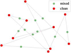
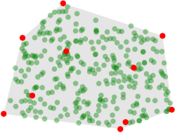
(a) mixup	(b) MultiMix (ours)

Figure 1: Data augmentation from a mini-batch $B$ consisting of $m=10$ points in two dimensions. (a) mixup: sampling of $m$ points on linear segments between $m$ pairs of points in $B$, using the same interpolation factor $\lambda$. (b) MultiMix: sampling of $n=300$ points in the convex hull of $B$.

In this work, we argue that a data augmentation process should augment the data seen by the model, or at least by its last few layers, as much as possible. In this sense, we follow manifold mixup [verma2019manifold] and generalize it in a number of ways to introduce MultiMix, as illustrated in Figure 1(b). First, rather than pairs, we interpolate tuples that are as large as the mini-batch. Effectively, instead of linear segments between pairs of examples in the mini-batch, we sample on their entire convex hull. Second, we draw a different vector $\lambda$ for each tuple. Third, and most important, we increase the number of interpolated tuples per iteration by orders of magnitude by only slightly decreasing the actual training throughput in examples per second. This is possible by interpolating at the deepest layer possible, i.e., just before the classifier, which also happens to be the most effective choice. The interpolated embeddings are thus only processed by a single layer.

Apart from increasing the number of examples seen by the model, another idea is to increase the number of loss terms per example. In many modalities of interest, the input is a sequence in one or more dimensions: pixels or patches in images, voxels in video, points or triangles in high-dimensional surfaces, to name a few. The structure of input data is expressed in matrices or tensors, which often preserve a certain spatial resolution until the deepest network layer before they collapse e.g. by global average pooling [SLJ+15, he2016deep] or by taking the output of a classification token [VSP+17, dosovitskiy2020image].

In this sense, we choose to operate at the level of sequence elements rather than representing examples by a single vector. We introduce dense MultiMix, which is the first approach of this kind in mixup-based data augmentation. In particular, we interpolate densely the embeddings and targets of sequence elements and we also apply the loss densely, as illustrated in LABEL:fig:dense. This is an extreme form of augmentation where the number of interpolated tuples and loss terms increases further by one or two orders of magnitude, but at little cost.

Finally, linear interpolation of targets, which is the norm in most mixup variants, has a limitation: Given two examples with different class labels, the interpolated example may actually lie in a region associated with a third class in the feature space, which is identified as manifold intrusion [guo2019mixup]. In the absence of any data other than the mini-batch, a straightforward way to address this limitation is to devise targets originating in the network itself. This naturally leads to self-distillation, whereby a moving average of the network acts as a teacher and provides synthetic soft targets [tarvainen2017mean], to be interpolated exactly like the original hard targets.

In summary, we make the following contributions:

1. We introduce MultiMix, which, given a mini-batch of size $m$, interpolates an arbitrary number $n\gg m$ of tuples, each of length $m$, with one interpolation vector $\lambda$ per tuple—compared with $m$ pairs, all with the same scalar $\lambda$ for most mixup methods (subsection 3.2).

2. We extend to dense interpolation and loss computation over all spatial positions (LABEL:sec:dense).

3. We use online self-distillation to generate and interpolate soft targets for mixup—compared with linear target interpolation for most mixup methods (subsection 3.3).

4. We improve over state-of-the-art mixup methods on image classification, robustness to adversarial attacks, object detection and out-of-distribution detection. (LABEL:sec:exp).

2 Related Work

Mixup

In general, mixup interpolates between pairs of input examples [zhang2018adversarial] or embeddings [verma2019manifold] and their corresponding target labels. Several follow-up methods mix input images according to spatial position, either at random rectangles [yun2019cutmix] or based on attention [uddin2020saliencymix, kim2020puzzle, kim2021co], in an attempt to focus on a different object in each image. We also use attention in our dense MultiMix variant, but in the embedding space. Other definitions of interpolation include the combination of content and style from two images [hong2021stylemix] and the spatial alignment of dense features [venkataramanan2021alignmix]. Our dense MultiMix variant also uses dense features but without aligning them, hence it can mix a very large number of images and generate even more interpolated data.

Our work is orthogonal to these methods as we focus on the sampling process of augmentation rather than on the definition of interpolation. As far as we are aware, the only methods that mix more than two examples are OptTransMix [zhu2020automix], which involves a complex optimization process in the input space and only applies to images with clean background, and SuperMix [Dabouei_2021_CVPR], which uses a Dirichlet distribution like we do, but interpolates in the input space not more than 3 images, while we interpolate all embeddings of a mini-batch.

Self-distillation

Distillation refers to a two-stage knowledge transfer process where a larger teacher model or ensemble is trained before predicting soft targets to train a smaller student model on the same [bucilua2006model, hinton2015distilling, romero2014fitnets, shen2019meal, zagoruyko2016paying] or different [RDG+18, xie2020self] training data. The architecture of the two models may be the same with training at multiple stages, for example in continual learning [rebuffi2017icarl, LiHo18]. In self-distillation or co-distillation, not only the models are the same, but the knowledge transfer process is also online, e.g. between layers of the same model [zhang2019your] or between two versions of the model [anil2018large], where the teacher parameters may be obtained from the student rather than learned [tarvainen2017mean]. The latter approach has been successful in self-supervised representation learning [grill2020bootstrap, caron2021emerging, zhou2021ibot]. As far as we know, distillation has only been used for mixup as a two stage process between different models [Dabouei_2021_CVPR] and we are the first to use online self-distillation in this context, following [tarvainen2017mean].

Dense loss functions

Although standard in dense tasks like semantic segmentation [noh2015learning, he2017mask], where dense targets commonly exist, dense loss functions are less common otherwise. Few examples are in few-shot learning [Lifchitz_2019_CVPR, Li_2019_CVPR], where data augmentation is of utter importance, and in unsupervised representation learning, e.g. dense contrastive learning [o2020unsupervised, Wang_2021_CVPR], learning from spatial correspondences [xiong2021self, xie2021propagate] and masked language or image modeling [bert, xie2021simmim, li2021mst, zhou2021ibot]. Some of these methods use dense distillation [xiong2021self, zhou2021ibot], which is also studied in continual learning [Dhar_2019_CVPR, DCO+20]. To our knowledge, we are the first to use dense interpolation and a dense loss function for mixup. Our setting is supervised, similar to dense classification [Lifchitz_2019_CVPR], but we also use dense distillation [zhou2021ibot].

3 Method

3.1 Preliminaries and background

Problem formulation

Let $x\in\mathcal{X}$ be an input example and $y\in\mathcal{Y}$ its one-hot encoded target, where $\mathcal{X}={}^{D}$ is the input space, $\mathcal{Y}=\{0,1\}^{c}$ and $c$ is the total number of classes. Let $f_{\theta}:\mathcal{X}\to{}^{d}$ be an encoder that maps the input $x$ to an embedding $z=f_{\theta}(x)$, where $d$ is the dimension of the embedding. A classifier $g_{W}:{}^{d}\to\Delta^{c-1}$ maps $z$ to a vector $p=g_{W}(z)$ of predicted probabilities over classes, where $\Delta^{n}\subset{}^{n+1}$ is the unit $n$-simplex, i.e., $p\geq 0$ and $\mathbf{1}_{c}^{\top}p=1$, and $\mathbf{1}_{c}\in{}^{c}$ is an all-ones vector. The overall network mapping is $f\mathrel{:=}g_{W}\circ f_{\theta}$.

Parameters $(\theta,W)$ are learned by optimizing over mini-batches. Given a mini-batch of $m$ examples, let $X=(x_{1},\dots,x_{m})\in{}^{D\times m}$ be the inputs, $Y=(y_{1},\dots,y_{m})\in{}^{c\times m}$ the targets and $P=(p_{1},\dots,p_{m})\in{}^{c\times m}$ the predicted probabilities of the mini-batch, where $P=f(X)\mathrel{:=}(f(x_{1}),\dots,f(x_{m}))$. The objective is to minimize the cross-entropy

$$H(Y,P)\mathrel{:=}-\mathbf{1}_{c}^{\top}(Y\odot\log(P))\mathbf{1}_{m}/m$$ (1)

of predicted probabilities $P$ relative to targets $Y$ averaged over the mini-batch, where $\odot$ is the Hadamard (element-wise) product. In summary, the mini-batch loss is

$$L(X,Y;\theta,W)\mathrel{:=}H(Y,g_{W}(f_{\theta}(X))).$$ (2)

Mixup

Mixup methods commonly interpolate pairs of inputs or embeddings and the corresponding targets at the mini-batch level while training. Given a mini-batch of $m$ examples with inputs $X$ and targets $Y$, let $Z=(z_{1},\dots,z_{m})\in{}^{d\times m}$ be the embeddings of the mini-batch, where $Z=f_{\theta}(X)$. Manifold mixup [verma2019manifold] interpolates the embeddings and targets by forming a convex combination of the pairs with interpolation factor $\lambda\in[0,1]$:

$$\widetilde{Z} =Z(\lambda I+(1-\lambda)\Pi)$$ (3)

$$\widetilde{Y} =Y(\lambda I+(1-\lambda)\Pi),$$ (4)

where $\lambda\sim\operatorname{Beta}(\alpha,\alpha)$, $I$ is the identity matrix and $\Pi\in{}^{m\times m}$ is a permutation matrix. Input mixup [zhang2018mixup] interpolates inputs rather than embeddings:

$$\widetilde{X}=X(\lambda I+(1-\lambda)\Pi).$$ (5)

Whatever the interpolation method and the space where it is performed, the interpolated data, e.g. $\widetilde{X}$ [zhang2018mixup] or $\widetilde{Z}$ [verma2019manifold], replaces the original mini-batch data and gives rise to predicted probabilities $\widetilde{P}=(p_{1},\dots,p_{m})\in{}^{c\times m}$ over classes, e.g. $\widetilde{P}=f(\widetilde{X})$ [zhang2018mixup] or $\widetilde{P}=g_{W}(\widetilde{Z})$ [verma2019manifold]. Then, the average cross-entropy $H(\widetilde{Y},\widetilde{P})$ (1) between the predicted probabilities $\widetilde{P}$ and interpolated targets $\widetilde{Y}$ is minimized.

The number of interpolated data is $m$, same as the original mini-batch data.

3.2 MultiMix

Interpolation

Given a mini-batch of $m$ examples with embeddings $Z$ and targets $Y$, we draw interpolation vectors $\lambda_{k}\sim\operatorname{Dir}(\alpha)$ for $k=1,\dots,n$, where $\operatorname{Dir}(\alpha)$ is the symmetric Dirichlet distribution and $\lambda_{k}\in\Delta^{m-1}$, that is, $\lambda_{k}\geq 0$ and $\mathbf{1}_{m}^{\top}\lambda_{k}=1$. We then interpolate embeddings and targets by taking $n$ convex combinations over all $m$ examples:

$$\widetilde{Z} =Z\Lambda$$ (6)

$$\widetilde{Y} =Y\Lambda,$$ (7)

where $\Lambda=(\lambda_{1},\dots,\lambda_{n})\in{}^{m\times n}$. We thus generalize manifold mixup [verma2019manifold]:

1. from pairs to tuples of length $m$, as long as the mini-batch: $m$-term convex combination (6),(7) vs. 2-term in (3),(4), Dirichlet vs. Beta distribution;

2. from $m$ to an arbitrary number $n$ of tuples: interpolated embeddings $\widetilde{Z}\in{}^{d\times n}$ (6) vs. ^d×m in (3), interpolated targets $\widetilde{Y}\in{}^{c\times n}$ (7) vs. ^c×m in (4);

3. from fixed $\lambda$ across the mini-batch to a different $\lambda_{k}$ for each interpolated item.

Loss

Again, we replace the original mini-batch embeddings $Z$ by the interpolated embeddings $\widetilde{Z}$ and minimize the average cross-entropy $H(\widetilde{Y},\widetilde{P})$ (1) between the predicted probabilities $\widetilde{P}=g_{W}(\widetilde{Z})$ and the interpolated targets $\widetilde{Y}$ (7). Compared with (2), the mini-batch loss becomes

$$L_{M}(X,Y;\theta,W)\mathrel{:=}H(Y\Lambda,g_{W}(f_{\theta}(X)\Lambda)).$$ (8)

3.3 MultiMix with self-distillation

Networks

We use an online self-distillation approach whereby the network $f\mathrel{:=}g_{W}\circ f_{\theta}$ that we learn becomes the student, whereas a teacher network $f^{\prime}\mathrel{:=}g_{W^{\prime}}\circ f_{\theta^{\prime}}$ of the same architecture is obtained by exponential moving average of the parameters [tarvainen2017mean, grill2020bootstrap]. The teacher parameters $(\theta^{\prime},W^{\prime})$ are not learned: We stop the gradient in the computation graph.

Views

Given two transformations $T$ and $T^{\prime}$, we generate two different augmented views $v=t(x)$ and $v^{\prime}=t^{\prime}(x)$ for each input $x$, where $t\sim T$ and $t^{\prime}\sim T^{\prime}$. Then, given a mini-batch of $m$ examples with inputs $X$ and targets $Y$, let $V=t(X),V^{\prime}=t^{\prime}(X)\in{}^{D\times m}$ be the mini-batch views corresponding to the two augmentations and $Z=f_{\theta}(V),Z^{\prime}=f_{\theta^{\prime}}(V^{\prime})\in{}^{d\times m}$ the embeddings obtained by the student and teacher encoders respectively.

Interpolation

We obtain the interpolated embeddings $\widetilde{Z},\widetilde{Z}^{\prime}$ from $Z,Z^{\prime}$ by (6) and targets $\widetilde{Y}$ from $Y$ by (7), using the same $\Lambda$. The predicted class probabilities are given by $\widetilde{P}=g_{W}(\widetilde{Z})$ and $\widetilde{P}^{\prime}=g_{W^{\prime}}(\widetilde{Z}^{\prime})$, again obtained by the student and teacher classifiers, respectively.

Loss

We learn parameters $(\theta,W)$ by minimizing a classification and a self-distillation loss:

$$\gamma H(\widetilde{Y},\widetilde{P})+(1-\gamma)H(\widetilde{P}^{\prime},\widetilde{P}),$$ (9)

where $\gamma\in[0,1]$. The former brings the probabilities $\widetilde{P}$ predicted by the student close to the targets $\widetilde{Y}$, as in (8). The latter brings $\widetilde{P}$ close to the probabilities $\widetilde{P}^{\prime}$ predicted by the teacher.