Visual Foresight With a Local Dynamics Model

Abstract

Model-free policy learning has been shown to be capable of learning manipulation policies which can solve long-time horizon tasks using single-step manipulation primitives. However, training these policies is a time-consuming process requiring large amounts of data. We propose the Local Dynamics Model (LDM) which efficiently learns the state-transition function for these manipulation primitives. By combining the LDM with model-free policy learning, we can learn policies which can solve complex manipulation tasks using one-step lookahead planning. We show that the LDM is both more sample-efficient and outperforms other model architectures. When combined with planning, we can outperform other model-based and model-free policies on several challenging manipulation tasks in simulation.

1 Introduction

Real-world robotic manipulation tasks require a robot to execute complex motion plans while interacting with numerous objects within cluttered environments. Due to the difficulty in learning good policies for these tasks, a common approach is to simplify policy learning by expressing the problem using more abstract (higher level) actions such as end-to-end collision-free motions combined with some motion primitive such as pick, place, push, etc. This is often called the spatial action space and is used by several authors including [36, 25, 32, 33]. By leveraging these open-loop manipulation primitives, model-free policy learning learns faster and can find better policies. However, a key challenge with this approach is that a large number of actions need to be considered at each timestep leading to difficulties in learning within a large $SE(2)$ workspace or an $SE(3)$ workspace of any size.

Due to these challenges, model-based policy learning presents an attractive alternative because it has the potential to improve sample efficiency [29, 7, 13]. Applying model-based methods to robotics, however, has been shown to be difficult and often requires reducing the high-dimensional states provided by sensors to low-dimensional latent spaces. While these methods have been successfully applied to a variety of robotic manipulation tasks [30, 17] they also require a large amount of training data (on the order of 10,000 to 100,000 examples).

This paper proposes the Local Dynamics Model (LDM) which learns the state-transition function for the pick and place primitives within the spatial action space. Unlike previous work which learns a dynamics model in latent space, LDM exploits the encoding of actions into image-space native to the spatial action space to instead learn an image-to-image transition function. Within this image space, we leverage both the localized effect of pick-and-place actions and the spatial equivariance property of top-down manipulation to dramatically improve the sample efficiency of our method. Due to this efficiency, the dynamics model quickly learns useful predictions allowing us to perform policy learning with a dynamics model which is trained from scratch alongside the policy. We demonstrate this through our use of a one-step lookahead planner which uses the state value function in combination with the LDM to solve many different complex manipulation tasks in simulation.

We make the following contributions. First, we propose the Local Dynamics Model, a novel approach to efficiently modelling environmental dynamics by restructuring the transition function. Second, we introduce a method which leverages the LDM to solve challenging manipulation tasks. Our experimental results show that our method outperforms other model-based and model-free. Our code is available at https://github.com/ColinKohler/LocalDynamicsModel.

2 Related Work

Robotic Manipulation:

Broadly speaking, there are two common approaches to learning manipulation policies: open-loop control and close-loop control. In closed-loop control, the agent controls the delta pose of the end-effector enabling fine-tune control of the manipulator. This end-to-end approach has been shown to be advantageous when examining contact-rich domains [18], [12], [14]. In contrast, agents in open-loop control apply predefined action primitives, such as pick, place, or push, to specified poses within the workspace. This tends to provide more data-efficient learning but comes at the cost of less powerful policies [21].

Spatial Action Space

The spatial action space is an open-loop control approach to policy learning for robotic manipulation. Within this domain, it is common to combine planar manipulation with a fully-convolutional neural network (FCN) which is used as a grasp quality metric [21] or, more generally, a action-value metric [36, 32]. This approach has been adapted to a number of different manipulation tasks covering a variety of action primitives [2, 19, 35].

Dynamics Modelling:

Model-Based RL improves data-efficiency by incorporating a learned dynamics model into policy training. Model-based RL has been successfully applied to variety of non-robotic tasks [7, 4, 13] but has seen more mixed success in robotics tasks. While model-based RL has been shown to work well in robotics tasks with low-dimensional state-spaces [30, 17], the high-dimensionality of visual state-spaces more commonly seen in robotic manipulation tends to harm performance. More modern approaches learn a mapping from image-space to some underlying latent space and learn a dynamics model which learns the transition function between these latent states [22, 16].

More recent work has examined image-to-image dynamics models similar to the video prediction models in computer vision [6]. However, these works typically deal with short-time horizon physics such as poking objects [1] or throwing objects [37]. Paxton et al. [24] and Hoque et al. [11] learn visual dynamics models for pick and place primitives but require a large amount of data and time to learn an accurate model. Our work is most closely related to [3] and [34]. In [2], Berscheid et al., learn a visual transition model using a GAN architecture but only learn pick and push primitives while still requiring a large amount of data. Additionally, they only examine a simple bin picking task in their experiments. Wu et al. [34] learn a visual foresight model tailored to a suction cup gripper and use it to solve various block rearrangement tasks. In contrast, we achieve similar sample efficiency using a more complicated parallel jaw gripper across a much more diverse set of objects and tasks.

3 Problem Statement

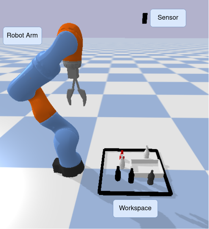
Figure 1: The Manipulation Scene

Manipulation as an MDP in a spatial action space:

This paper focuses on robotic manipulation problems expressed as a Markov decision process in a spatial action space, $\mathcal{M}=(S,A,T,R,\gamma)$, where state is a top down image of the workspace paired with an image of the object currently held in the gripper (the in-hand image) and action is a subset of $SE(2)$. Specifically, state is a pair of $c$-channel images, $s=(s_{scene},s_{hand})\in S_{scene}\times S_{hand}$, where $s_{scene}\in S_{scene}\subseteq\mathbb{R}^{c\times h\times w}$ is a $c\times h\times w$ image of the scene and $s_{hand}\in S_{hand}\subseteq\mathbb{R}^{c\times d\times d}$ is a $c\times d\times d$ image patch that describes the contents of the hand (Figure 2). At each time step, $s_{scene}$ is set equal to a newly acquired top-down image of the scene. $s_{hand}$ is set to the oriented $d\times d$ image patch corresponding to the pose of the last successful pick. If no successful pick has occurred or the hand is empty, then $s_{hand}$ is set to be the zero image. Action $a\in A\subseteq SE(2)$ is a target pose for an end effector motion to be performed at the current timestep. If action $a$ executes when the hand is holding an object (when the in-hand image is not zero), then $a$ is interpreted as a place action, i.e. move and then open the fingers. Otherwise, $a$ is interpreted as a pick, i.e. move and close the fingers. Here, $A=A_{pos}\times S^{1}\subseteq SE(2)$ spans the robot workspace and $A_{pos}\subseteq\mathbb{R}^{2}$ denotes the position component of that workspace. State and action are related to each other in that each action corresponds to the pixel in the state that is beneath the end effector target pose specified by the action. We assume we have access to a function $h:A\rightarrow\mathbb{Z}^{2}$ that maps an action to the pixel corresponding to its position component.

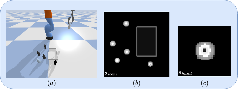
Figure 2: MDP State. (a) The manipulation scene. (b) The top-down image of the workspace, $s_{scene}$. (c) The in-hand image, $s_{hand}$.

Assumptions:

The following assumptions can simplify policy learning and are often reasonable in robotics settings. First, we assume that we can model transitions with a deterministic function. While manipulation domains can be stochastic, we note that high value transitions are often nearly deterministic, e.g. a high value place action often leads to a desired next state nearly deterministicly. As a result, planning with a deterministic model is often reasonable.

Assumption 1 (Deterministic Transitions)

The transition function is deterministic and can therefore be modeled by the function $s^{\prime}=f(s,a)$, i.e. the dynamics model.

The second assumption concerns symmetry with respect to translations and rotations of states and actions. Given a transformation $g\in SE(2)$, $g(s)$ denotes the state $s=(s_{scene},s_{hand})$ where $s_{scene}$ has been rotated and translated by $g$ and $s_{hand}$ is unchanged. Similarly, $g(a)$ denotes the action $a$ rotated and translated by $g$.

Assumption 2 ($SE(2)$ Symmetric Transitions)

The transition function is invariant to translations and rotations. That is, for any translation and rotation $g\in SE(2)$, $T(s,a,s^{\prime})=T(g(s),g(a),g(s^{\prime}))$ for all $s,a,s^{\prime}\in S\times A\times S$.

The last assumption concerns the effect of an action on state. Let $R\subseteq A_{pos}$ be a region of $\mathbb{R}^{2}$. Given a state $s=(s_{scene},s_{hand})$, let $s^{\prime}_{scene}=\textsc{mask}(s,R)\in S_{scene}$ denote the scene image that is equal to $s_{scene}$ except that all pixels inside $R$ have been masked to zero. In the following, we will be exclusively interested in image masks involving the region $B_{a}$, defined as follows:

Definition 3.1 (Local Region).

For an action $a=(a_{pos},a_{\theta})\in\mathrm{SE}(2)$, let $B_{a}\subseteq A_{pos}$ denote the square region with a fixed side length $d$ (a hyperparameter) that is centered at $a_{pos}$ and oriented by $a_{\theta}$.

We are now able to state the final assumption:

Assumption 3 (Local Effects)

An action $a\in A$ does not affect parts of the scene outside of $B_{a}$. That is, given any transition $s^{\prime}=f(s,a)$, it is the case that $\textsc{mask}(s,B_{a})=\textsc{mask}(s^{\prime},B_{a})$.

The bottle arrangement task (Figures 1, 2) is an example of a robotic manipulation domain that satisfies the assumptions above. First, notice that high value actions in this domain lead to deterministic pick and place outcomes, i.e. picking up the bottle and placing it with a low probability of knocking it over. Second, notice that transitions are rotationally and translationally symmetric in this problem. Finally, notice that interactions between the hand and the world have local effects. If the hand grasps or knocks over a bottle, that interaction typically affects only objects nearby the interaction.

4 Method

In this section, we first introduce the Local Dynamics Model (LDM) detailing its properties and model architecture. We then discuss how we combine the LDM with an action proposal method to perform policy learning through one-step lookahead planning.

4.1 Structuring the Transition Model

We simplify the problem of learning the transition function $f:S\times A\rightarrow S$ by encoding Assumptions 2 and 3 as constraints on the model as follows. First, given a state $s=(s_{scene},s_{hand})$, we partition the scene image $s_{scene}$ into a region that is invariant under $a$, $\check{s}_{a}=\textsc{mask}(s,B_{a})$, and a region that changes under $a$, $\hat{s}_{a}=\textsc{crop}(s,B_{a})$. Here, $\textsc{crop}(s,R)\in\mathbb{R}^{c\times d\times d}$ denotes the $c$-channel $d\times d$ image patch cropped from $s_{scene}$ corresponding to region $R\subseteq A_{pos}$, resized to a $d\times d$ image. Using this notation, we can reconstruct the original scene image by combining $\hat{s}_{a}$ and $\check{s}_{a}$:

$$s_{scene}=\textsc{insert}(\hat{s}_{a},B_{a})+\check{s}_{a},$$ (1)

where $\hat{s}_{a}=\textsc{crop}(s,B_{a})$ and $\textsc{insert}(\hat{s}_{a},B_{a})$ inserts the crop into region $B_{a}$ and sets the pixels outside $B_{a}$ to zero.

4.2 Local Dynamics Model

 

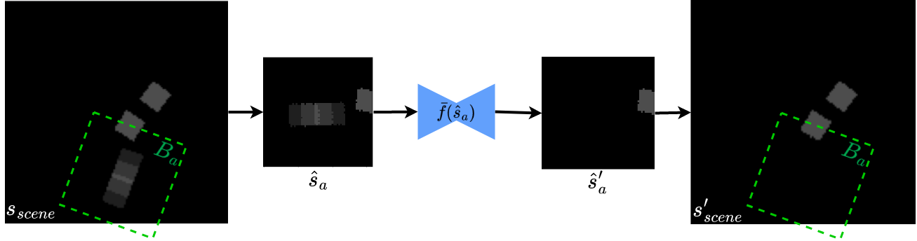
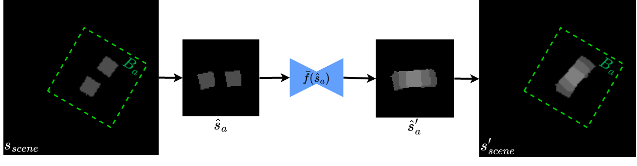
Figure 3: Local dynamics model. In order to predict the next scene image $s^{\prime}_{scene}$, we learn a model $\bar{f}$ that predicts how the scene will change within $B_{a}$, a neighborhood around action $a$. The output of this model is inserted into the original scene image.

Instead of learning $f$ directly, we will learn a function $\bar{f}:\mathbb{R}^{c\times d\times d}\rightarrow\mathbb{R}^{c\times d\times d}$ that maps the image patch $\hat{s}_{a}$ onto a new patch $\hat{s}^{\prime}_{a}$. Whereas $f$ models the dynamics of the entire scene, $\bar{f}$ only models changes in the scene within the local region $B_{a}$. We refer to $\bar{f}$ as the local dynamics model (LDM). Given such a model, we can define a function $f_{scene}$ as:

$$f_{scene}(s,a)=\textsc{insert}(\bar{f}(\hat{s}_{a}),B_{a})+\check{s}_{a},$$ (2)

where $\hat{s}_{a}=\textsc{crop}(s,B_{a})$. We can reconstruct $f$ as $f(s,a)=(f_{scene}(s,a),s^{\prime}_{hand})$ where $s^{\prime}_{hand}$ denotes the in-hand image obtained using the rules described in Section 3. Figure 3 illustrates this process for picking and placing in a block arrangement task.

Notice that the model in Equation 2, $f_{scene}$, satisfies both Assumptions 2 and 3. The fact that it satisfies Assumption 3 is easy to see as the local dynamics model $\bar{f}$ only models changes in the scene within the local region $B_{a}$. It also satisfies Assumption 2 because $\hat{s}_{a}$ is invariant under transformations $g\in\mathrm{SE}(2)$ of $s$ and $a$:

$$\hat{s}_{a} =\textsc{crop}(s,B_{a})$$

$$=\textsc{crop}(g(s),B_{g(a)}),$$

where $g(s)$ rotates state $s$ and $g(a)$ rotates action $a$. As a result, Equation 2 is constrained to be equivariant in the sense that $g(f_{scene}(s,a))=f_{scene}(g(s),g(a))$.

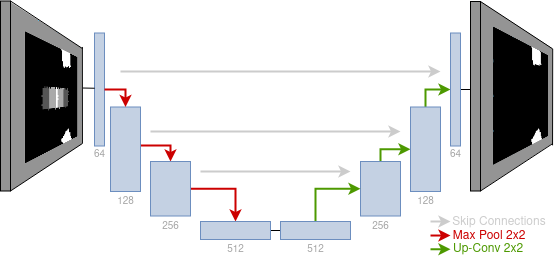
Figure 4: LDM architecture. Model architecture used in $\bar{f}$, the local dynamics model. Each blue box represents a 3x3 ResNet Block.

Model Architecture:

We model the local dynamics model, $\bar{f}$, using the UNet model architecture shown in Figure 4 with four convolution and four deconvolution layers. It takes as input the image patch $\hat{s}_{a}\in\mathbb{R}^{c\times d\times d}$, and outputs a patch from the predicted next state, $\hat{s}^{\prime}_{a}\in\mathbb{R}^{c\times d\times d}$. The size of this image patch must be large enough to capture the effects of pick and place actions, but small enough to ignore objects not affected by the current interaction. In our experiments, we set $d=64$ pixels which corresponds to roughly $20cm$ in the workspace.

Loss Function:

$\bar{f}$ is trained using a reconstruction loss, i.e. a loss which measures the difference between a predicted new state image patch and a ground truth image patch. Typically, this is accomplished using a pixel-wise L2 loss [10]. However, we instead model pixel values as a multinomial probability distribution over 21 different possible values for each pixel (in our case, these are depth values since we use depth images). This enables us to use a cross entropy loss, which has been shown to have better performance relative to an L2 loss [31]. We were able to improve performance even further by using a focal loss rather than a vanilla cross entropy loss [20]. This alleviates the large class imbalance issues that arise from most pixels in $\hat{s}_{a}$ having the same value and focuses learning on parts of the pixel space with the most challenging dynamics.

4.3 Policy Learning

While there are a variety of ways to improve policy learning using a dynamics model, here we take a relatively simple one-step lookahead approach. We learn the state value function $V_{\psi}(s)$, and use it in combination with the dynamics model to estimate the $Q$ function, $\hat{Q}(s,a)=V_{\psi}(f(s,a))$. A key challenge here is that it is expensive to evaluate $\max_{a\in A}\hat{Q}(s,a)$ or $\arg\max_{a\in A}\hat{Q}(s,a)$ over large action spaces (such as the spatial action space) because the forward model must be queried separately for each action. We combat this problem by learning an approximate $Q$ function that is computationally cheap to query and use it to reduce the set of actions over which we maximize. Specifically, we learn a function $Q_{\theta}$ using model-free $Q$-learning: $Q_{\theta}(s,a)\leftarrow r+\gamma\max_{a^{\prime}\in A}Q_{\theta}(s^{\prime},a^{\prime})$. Then, we define a policy $\pi_{\theta}(a|s)=\sigma_{A}(Q_{\theta}(s,a))$, where $\sigma_{A}$ denotes the softmax function over the action space $A$ with an implicit temperature parameter $\tau$. We sample a small set of high quality actions $\bar{A}_{N}\subseteq A$ by drawing $N$ action samples from $\pi_{\theta}(a|s)$. Now, we can approximate $\max_{a\in A}\hat{Q}(s,a)\approx\max_{a\in\bar{A}_{N}}\hat{Q}(s,a)$. The target for learning $V_{\psi}$ is now $V_{\psi}(s)\leftarrow r+\max_{a\in\bar{A}_{N}}\hat{Q}(s,a)$. The policy under which our agent acts is $\pi(a|s)=\sigma_{\bar{A}_{N}}(\hat{Q}(s,a))$. We schedule exploration by decreasing the softmax temperature parameter over the course of learning.

We model $Q_{\theta}$ using a fully-convolutional neural network which takes as input the top-down heightmap $s_{scene}$ and outputs a 2-channel action-value map $(Q_{pick},Q_{place})\in\mathbb{R}^{2\times r\times h\times w}$ where $Q_{pick}$ correlates with picking success and $Q_{place}$ to placing success. The orientation of the action is represented by discretizing the space of $SO(2)$ rotations into $r$ values and rotating $s$ by each $\theta$ value. $V_{\psi}$ is modeled as standard convolutional neural network which takes the state $s$ as input and outputs the value of that state. We use two target networks parameterized by $\theta^{-}$ and $\psi^{-}$ which are updated to the current weights $\theta$ and $\psi$ every $t$ steps to stabilize training.

4.4 Sampling Diverse Actions

When evaluating $\max_{a\in\bar{A}_{N}}\hat{Q}(s,a)$ and $\pi(a|s)=\sigma_{\bar{A}_{N}}(\hat{Q}(s,a))$, it is important to sample a diverse set of actions $\bar{A}_{N}$. The problem is that $\sigma(Q_{\theta},\cdot))$ can sometimes be a low entropy probability distribution with a small number of high-liklihood peaks. If we draw $N$ independent samples directly from this distribution, we are likely to obtain multiple near-duplicate samples. This is unhelpful since we only need one sample from each mode in order to evaluate it using $V_{\psi}(f(s,a))$. A simple solution would be to sample without replacement. Unfortunately, as these peaks can include a number of actions, we would have to draw a large number of samples in order to ensure this diversity. To address this problem, we use an inhibition technique similar to non-maximum suppression where we reduce the distribution from which future samples are drawn in a small region around each previously drawn sample. Specifically, we draw a sequence of samples, $a_{1},\dots,a_{N}$. The first sample is drawn from the unmodified distribution $Q_{\theta}(s,\cdot)$. Each successive sample $j\neq N$ is drawn from a distribution $Q_{\theta}(s,\cdot)-\beta\sum_{i=1}^{j}\mathcal{N}(a_{i},\sigma^{2})$, where $\mathcal{N}$ denotes the standard normal distribution in $\mathbb{R}^{3}$, and $\beta$ and $\sigma^{2}$ are constants. Here, we have approximated $\mathrm{SE}(2)$ as a vector space $\mathbb{R}^{3}$ in order to apply the Gaussian. Over the course of training, we slowly reduce $\beta$ as the optimal policy is learned.

5 Experiments

We performed a series of experiments to test our method. First, we investigate the effectiveness of the Local Dynamics Model (LDM) by training the model in isolation on pre-generated offline data. Second, we demonstrate that we can learn effective policies across a number of complex robotic manipulation tasks.

Network Architecture:

A classification UNet with bottleneck Resnet blocks [8] is used as the architecture of the LDM. A similar network architecture is used for the Q-value model, $Q_{\theta}$, with the exception of using basic Resnet blocks. The state value model, $V_{\psi}$, is a simple CNN with basic Resnet blocks and two fully-connected layers. The exact details for the number of layers and hidden units can be found in our Github repository.

Implementation Details:

The workspace has a size of $0.4m\times 0.4m$ and $s_{scene}$ covers the workspace with a heightmap of size of $128\times 128$ pixels. We use $8$ discrete rotations equally spaced from $0$ to $\pi$. The target network is synchronized every 100 steps. We used the Adam optimizer [15], and the best learning rate and its decay were chosen to be $10^{-3}$ and $0.95$ respectively. The learning rate is multiplied by the decay every $2000$ steps. We use the prioritized replay buffer [28] with prioritized replay exponent $\alpha=0.6$ and prioritized importance sampling exponent $B_{0}=0.0$ annealed to $1$ over training. The expert transitions are given a priority bonus of $\epsilon_{d}=1$ as in Hester et al. [9]. The buffer has a size of $10000$ episodes. Our implementation is based on PyTorch [23].

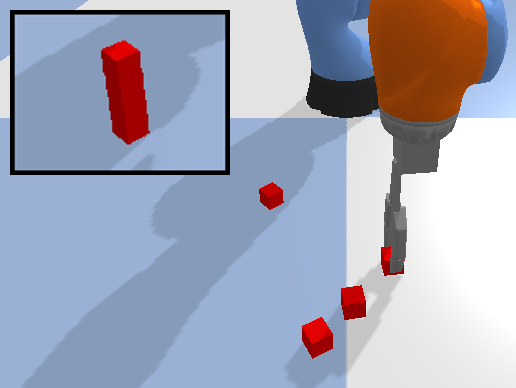
(a) Block Stacking

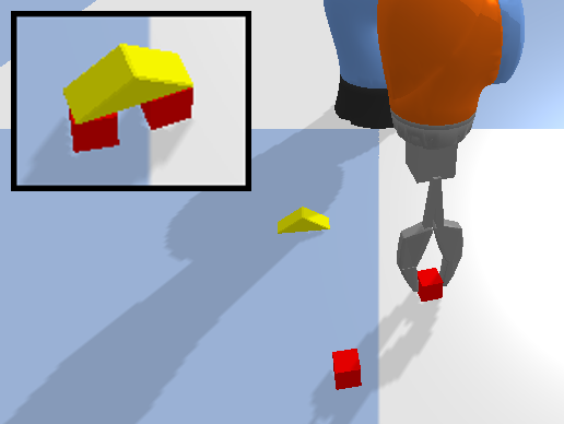
(b) House Building

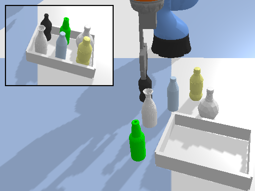
(c) Bottle Arrange

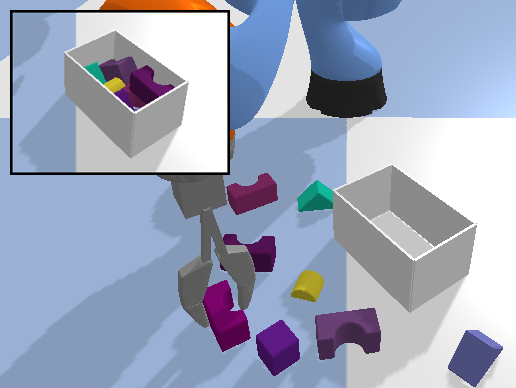
(d) Bin Packing

Figure 5: Tasks. The window in the top-left corner shows the goal state.

Task Descriptions:

For all experiments, both the training and testing is preformed in the PyBullet simulator [5]. In the block stacking domain, three cubes are placed randomly within the workspace and the agent is tasked with placing these blocks into a stable stack. In the house building domain, two cubes and one triangle are placed randomly within the workspace and the agent is tasked with placing the triangle on top of the two cube blocks. In the bottle arrangement domain, the agent needs to gather six bottles in a tray. These three environments have spare rewards ($+1$ at goal and $0$ otherwise).

In the bin packing domain, the agent must compactly pack eight blocks into a bin while minimizing the height of the pack. This environment uses a richer reward function and provides a positive reward with magnitude inversely proportional to the highest point in the pile after packing all objects. Example initial and goal configurations for these domains can be seen in Figure 5.

5.1 Accuracy of the Local Dynamics Model

	Block Stacking			House Building
Method	L1	SR		L1	SR
Naive	$30.3\pm 1.7$	$38\pm 5.6$		$30.4\pm 1.5$	$39.1\pm 1.9$
LDM(128)	$14.5\pm 2.2$	$70\pm 1.8$		$10.9\pm 0.24$	$70.7\pm 0.6$
LDM(64)	$\mathbf{8.76\pm 0.1}$	$\mathbf{83.4\pm 0.6}$		$\mathbf{5.88\pm 0.2}$	$\mathbf{77.9\pm 1.1}$
	Bottle Arrangement			Bin Packing
Method	L1	SR		L1	SR
Naive	$48.9\pm 0.9$	$43.8\pm 4.4$		$77.2\pm 0.71$	$35.4\pm 0.8$
LDM(128)	$43.6\pm 0.79$	$58.6\pm 1.3$		$93.3\pm 1.9$	$60.4\pm 2.1$
LDM(64)	$\mathbf{32.5\pm 1.8}$	$\mathbf{66\pm 1.9}$		$\mathbf{48.8\pm 0.9}$	$\mathbf{65.9\pm 0.5}$

Table 1: Dynamics Model Performance. Final performance for the $4$ domains on the different dynamics models. The results show the mean and standard deviation averaged over 3 random seeds. L1 denotes the L1-pixelwise difference between the predicted observation and the true observation. Lower is better. SR denotes the success rate (%) for the action. Higher is better.

Experiment:

We generate $5$k steps of noisy expert data for each of the domains in Figure 5 by rolling out a hand coded stochastic policy. For the block stacking and house building domains we train the models for $5$k iterations of optimization. For the bottle arrangement and bin packing domains we train the models for $10$k iterations.

Metrics:

We examine two metrics of model accuracy: 1.) the L1-pixelwise difference between the predicted observation and the true observation and 2.) the success rate of the action primitives. A pick action is defined as a success if the model correctly predicts if the object will be picked up or not. Similarly, a place action is defined as a success provided the model correctly predicts the pose of the object after placement. The L1 difference provides a low level comparison of the models whereas the success rate provides a higher level view which is more important for planning and policy learning.

Baselines:

We compare the performance of three dynamics models.

1. LDM(64): Local Dynamics Model with a crop size of $64$ pixels.

2. LDM(128): Local Dynamics Model with a crop size of $128$ pixels.

3. Naive: UNet forward model with $128\times 128$ input and output size. The action is encoded by concatenating a binary mask of the action position onto the state $s$.

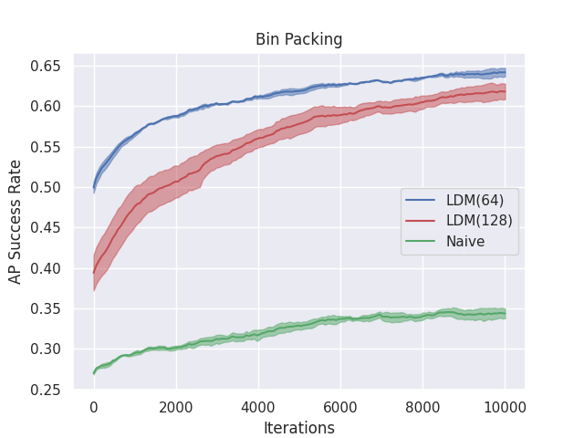
Figure 6: Sample Efficiency. Action primitive success rate for bin packing. Results averaged over three random seeds. Shading denotes standard error.

Results:

In Table 1, we summarize the accuracy of the models in the four domains on a held-out test set. While both LDM(64) and LDM(128) are able to generate realistic images in non-cluttered domains, we find that defining a small localized area of affect to be vital in cluttered domains such as bin packing. The most common failure mode occurs when the model overestimates the stability of object placements. For example, it has difficulties in determining the inflection point when stacking blocks which will lead to the stack falling over. Equally important to the final performance of the models is how efficiently they learn. In Figure 6, the action primitive success rate is shown over training for the bin packing environment. The sample efficiency of LDM(64) makes it much more useful for policy learning as the faster the dynamics model learns the faster the policy will learn.

5.2 Policy Learning

Here, we evaluate our ability to use the local dynamics model to learn policies that solve the robotic manipulation tasks illustrated in Figure 5. In each of these domains, the robot must execute a series of pick and place actions in order to arrange a collection of objects as specified by the task. These are sparse reward tasks where the agent gets a non-zero reward only upon reaching a goal state. As such, we initialize the replay buffer for all agents with $100$ expert demonstration episodes in order to facilitate exploration.

Baselines:

We compare our approach with the following baselines.

1. FC-DQN: Model-free policy learning using a fully-convolutional neural network to predict the q-values for each action in the spatial-action space. Rotations are encoded by rotating the input and output for each $\theta$ [36].

2. Random Shooing (RS): RS samples $K$ candidate action sequences from a uniform distribution and evaluates each candidate using the dynamics module. The optimal action sequence is chosen as the one with the highest return [27, 26]. Due to the size of the action space, we restrict action sampling to only sample actions which are nearby or on obejcts within the workspace.

3. Dyna-Q: FC-DQN model trained Dyna-style where training iterates between two steps. First, data is gathered using the current policy and used to learn the dynamics model. Second, the policy is improved using synthetic data generated by the dynamics model. At test time only the policy is used [29].

For fairness, all algorithms use the same model architecture. For RS and Dyna-Q, an extra head is added onto the state value model after the feature extraction layers in order to predict the reward for that state. When a model is not used, such as the value model for RS, they are not trained during that run. The forward model is not pretrained in any of the algorithms considered. All algorithms begin training the forward model online using the on-policy data contained in the replay buffer – the same data used to train the policy.

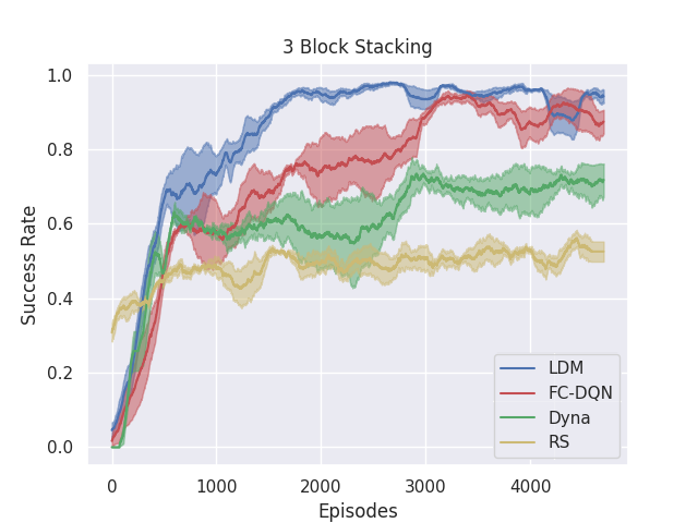
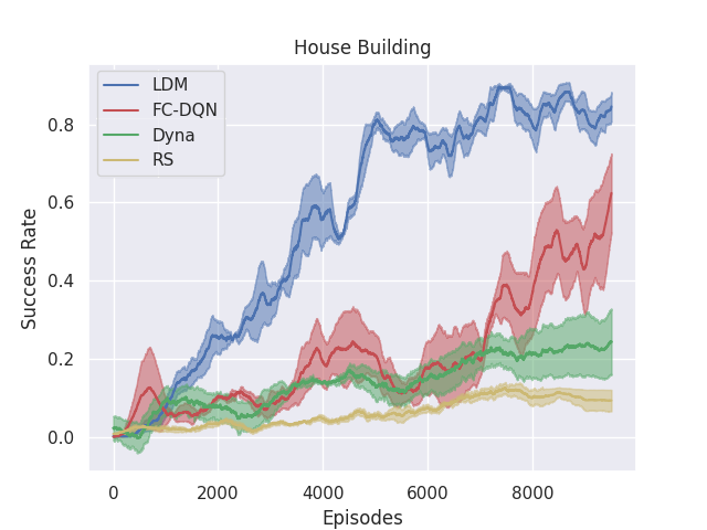
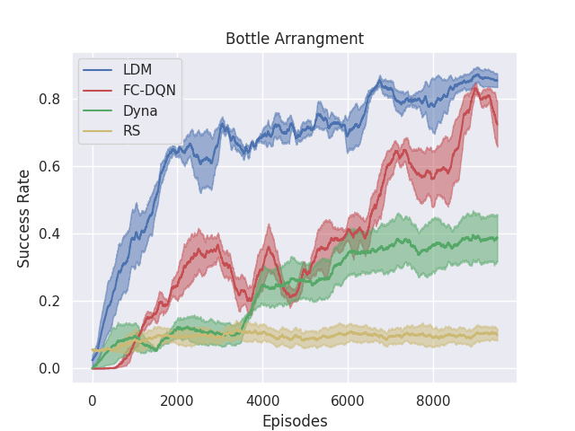
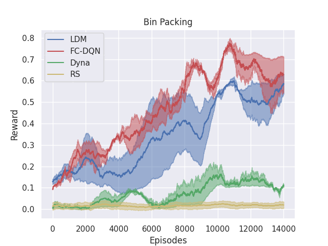
Figure 7: Simulation Experiment Evaluation. Evaluation performance of greedy-policy. Models are trained until LDM reaches convergence. Results averaged over 3 random seeds. Shading denotes standard error.

Results:

The results are summarized in Figure 7. They show that our method (shown in blue) is more sample efficient than FC-DQN in all domains except bin packing. We attribute the under-performance in bin packing to the difficult transition function that the state prediction model must learn due to the varied geometry of the blocks interacting with each other. LDM significantly out-preforms the model-based baselines in all domains. RS preforms poorly even with a high quality state prediction model due to the low probability of randomly sampling a good trajectory in large actions spaces. Dyna-Q performs similarly poorly due to the minute differences between the simulated experiences and the real experiences cause the policy learned to preform worse on real data.

5.3 Generalization

	Block Stacking			Bottle Arrangement
Method	4 Block	5 Block		5 Bottle	6 Bottle
RS	48	23		8	4
FC-DQN	98	89		82	48
LDM	99	84		86	65

Table 2: Generalization Experiment. We show the success rate (%) of zero-shot generalization over 100 episodes. Higher is better.

One advantageous property of model-based RL, is its ability to generalize to unseen environments provided the underlying dynamics of the environments remains similar. In order to test how well LDM generalizes, we trained LDM, FC-DQN, and RS on the block stacking and bottle arrangement domains on a reduced number of objects and evaluated them with an increased number of objects, i.e. zero-shot generalization. Specifically, we trained our models on 3 block stacking and evaluated them on 4 and 5 block stacking. Similarly, we trained our models on 4 bottle arrangement and evaluated them on 5 and 6 bottle arrangement. As shown in Table 2, LDM is more effective for zero-shot generalization when compared to both the model-free (FC-DQN) and model-based (RS) baselines.

6 Limitations and Future Work

This work has several limitations and directions for future research. The most glaring of these is our use of a single-step lookahead planner for policy learning. One large advantage of model-based methods is their ability to plan multiple steps ahead to find the most optimal solution. For instance in bin packing, our single-step planner will occasionally greedily select a poor action which results in the final pack being taller whereas a multi-step planner would be able to avoid this action by examining the future consequences. Similarly, model-based methods have been shown to work well in multi-task learning where a more general model is learned and leveraged across a number of tasks. While we show that we can use the LDM for zero-shot generalization, our planning approach is more tailored to learning single-policies. The LDM on the other hand, is shown to be capable of modeling the interactions between many different objects across many different tasks making it ideal for use in multi-task learning.

In terms of the LDM, we believe their are two interesting avenues for future work. First, due to our modeling of the pixels as probability distributions, we can easily estimate the uncertainty of the LDM’s predictions by calculating the pixelwise entropy of the model output. This could prove useful when planning by allowing us to avoid taking actions which the LDM is more uncertain about leading to more robust solutions. Secondly, although we encode $SE(2)$ equivariance into the LDM by restructuring the dynamics function, we could also explore the use of equivriatant CNNs in the LDM architecture. These equviariant CNNs have been shown to greatly improve sample efficiency across a wide number of tasks and have recently started being applied to robotic manipulation tasks similar to those we present in this work.

7 Conclusion

In this paper, we propose the Local Dynamics Model (LDM) approach to forward modeling which learns the state-transition function for pick and place manipulation primitives. The LDM is able to efficiently learn the dynamics of many different objects faster and more accurately compared to similar methods. This sample efficiency is achieved by restructuring the transition function to make the LDM invariant to both objects outside the region near the action and to transformations in $SE(2)$. We show that the LDM can be used to solve a number of complex manipulation tasks through the use of a single-step lookahead planning method. Through the combination of the LDM with our planning method which samples a diverse set of actions, our proposed method is able to outperform the model-free and model-based baselines examined in this work.

References

- Agrawal et al. [2016] P. Agrawal, A. Nair, P. Abbeel, J. Malik, and S. Levine. Learning to poke by poking: Experiential learning of intuitive physics. arXiv preprint arXiv:1606.07419, 2016.
- Berscheid et al. [2019] L. Berscheid, P. Meißner, and T. Kröger. Robot learning of shifting objects for grasping in cluttered environments. In 2019 IEEE/RSJ International Conference on Intelligent Robots and Systems (IROS), pages 612–618. IEEE, 2019.
- Berscheid et al. [2021] L. Berscheid, P. Meißner, and T. Kröger. Learning a generative transition model for uncertainty-aware robotic manipulation. In 2021 IEEE/RSJ International Conference on Intelligent Robots and Systems (IROS), pages 4670–4677. IEEE, 2021.
- Chua et al. [2018] K. Chua, R. Calandra, R. McAllister, and S. Levine. Deep reinforcement learning in a handful of trials using probabilistic dynamics models. CoRR, abs/1805.12114, 2018. URL http://arxiv.org/abs/1805.12114.
- Coumans and Bai [2016–2021] E. Coumans and Y. Bai. Pybullet, a python module for physics simulation for games, robotics and machine learning. http://pybullet.org, 2016–2021.
- Finn and Levine [2016] C. Finn and S. Levine. Deep visual foresight for planning robot motion. CoRR, abs/1610.00696, 2016. URL http://arxiv.org/abs/1610.00696.
- Gu et al. [2016] S. Gu, T. Lillicrap, I. Sutskever, and S. Levine. Continuous deep q-learning with model-based acceleration. In International conference on machine learning, pages 2829–2838. PMLR, 2016.
- He et al. [2015] K. He, X. Zhang, S. Ren, and J. Sun. Deep residual learning for image recognition. CoRR, abs/1512.03385, 2015. URL http://arxiv.org/abs/1512.03385.
- Hester et al. [2017] T. Hester, M. Vecerík, O. Pietquin, M. Lanctot, T. Schaul, B. Piot, A. Sendonaris, G. Dulac-Arnold, I. Osband, J. P. Agapiou, J. Z. Leibo, and A. Gruslys. Learning from demonstrations for real world reinforcement learning. CoRR, abs/1704.03732, 2017. URL http://arxiv.org/abs/1704.03732.
- Hinton and Salakhutdinov [2006] G. E. Hinton and R. R. Salakhutdinov. Reducing the dimensionality of data with neural networks. science, 313(5786):504–507, 2006.
- Hoque et al. [2020] R. Hoque, D. Seita, A. Balakrishna, A. Ganapathi, A. K. Tanwani, N. Jamali, K. Yamane, S. Iba, and K. Goldberg. Visuospatial foresight for multi-step, multi-task fabric manipulation. arXiv preprint arXiv:2003.09044, 2020.
- Jang et al. [2017] E. Jang, S. Vijayanarasimhan, P. Pastor, J. Ibarz, and S. Levine. End-to-end learning of semantic grasping, 2017.
- Kaiser et al. [2019] L. Kaiser, M. Babaeizadeh, P. Milos, B. Osinski, R. H. Campbell, K. Czechowski, D. Erhan, C. Finn, P. Kozakowski, S. Levine, A. Mohiuddin, R. Sepassi, G. Tucker, and H. Michalewski. Model-based reinforcement learning for atari, 2019. URL https://arxiv.org/abs/1903.00374.
- Kalashnikov et al. [2018] D. Kalashnikov, A. Irpan, P. Pastor, J. Ibarz, A. Herzog, E. Jang, D. Quillen, E. Holly, M. Kalakrishnan, V. Vanhoucke, and S. Levine. Qt-opt: Scalable deep reinforcement learning for vision-based robotic manipulation, 2018.
- Kingma and Ba [2014] D. P. Kingma and J. Ba. Adam: A method for stochastic optimization. arXiv preprint arXiv:1412.6980, 2014.
- Kossen et al. [2019] J. Kossen, K. Stelzner, M. Hussing, C. Voelcker, and K. Kersting. Structured object-aware physics prediction for video modeling and planning, 2019. URL https://arxiv.org/abs/1910.02425.
- Lenz et al. [2015] I. Lenz, R. A. Knepper, and A. Saxena. Deepmpc: Learning deep latent features for model predictive control. In Robotics: Science and Systems. Rome, Italy, 2015.
- Levine et al. [2016] S. Levine, P. Pastor, A. Krizhevsky, and D. Quillen. Learning hand-eye coordination for robotic grasping with deep learning and large-scale data collection, 2016.
- Liang et al. [2019] H. Liang, X. Lou, and C. Choi. Knowledge induced deep q-network for a slide-to-wall object grasping. arXiv preprint arXiv:1910.03781, pages 1–7, 2019.
- Lin et al. [2017] T.-Y. Lin, P. Goyal, R. Girshick, K. He, and P. Dollar. Focal loss for dense object detection. In Proceedings of the IEEE International Conference on Computer Vision (ICCV), Oct 2017.
- Mahler et al. [2019] J. Mahler, M. Matl, V. Satish, M. Danielczuk, B. DeRose, S. McKinley, and K. Goldberg. Learning ambidextrous robot grasping policies. Science Robotics, 4(26):eaau4984, 2019.
- Minderer et al. [2019] M. Minderer, C. Sun, R. Villegas, F. Cole, K. P. Murphy, and H. Lee. Unsupervised learning of object structure and dynamics from videos. Advances in Neural Information Processing Systems, 32, 2019.
- Paszke et al. [2019] A. Paszke, S. Gross, F. Massa, A. Lerer, J. Bradbury, G. Chanan, T. Killeen, Z. Lin, N. Gimelshein, L. Antiga, et al. Pytorch: An imperative style, high-performance deep learning library. Advances in neural information processing systems, 32, 2019.
- Paxton et al. [2019] C. Paxton, Y. Barnoy, K. Katyal, R. Arora, and G. D. Hager. Visual robot task planning. In 2019 international conference on robotics and automation (ICRA), pages 8832–8838. IEEE, 2019.
- Platt et al. [2019] R. Platt, C. Kohler, and M. Gualtieri. Deictic image mapping: An abstraction for learning pose invariant manipulation policies. In Proceedings of the AAAI Conference on Artificial Intelligence, volume 33, pages 8042–8049, 2019.
- Richards [2005] A. G. Richards. Robust constrained model predictive control. PhD thesis, Massachusetts Institute of Technology, 2005.
- Ross et al. [2011] S. Ross, G. Gordon, and D. Bagnell. A reduction of imitation learning and structured prediction to no-regret online learning. In Proceedings of the fourteenth international conference on artificial intelligence and statistics, pages 627–635. JMLR Workshop and Conference Proceedings, 2011.
- Schaul et al. [2016] T. Schaul, J. Quan, I. Antonoglou, and D. Silver. Prioritized experience replay, 2016.
- Sutton [1991] R. S. Sutton. Dyna, an integrated architecture for learning, planning, and reacting. ACM Sigart Bulletin, 2(4):160–163, 1991.
- Tassa et al. [2018] Y. Tassa, Y. Doron, A. Muldal, T. Erez, Y. Li, D. d. L. Casas, D. Budden, A. Abdolmaleki, J. Merel, A. Lefrancq, T. Lillicrap, and M. Riedmiller. Deepmind control suite, 2018. URL https://arxiv.org/abs/1801.00690.
- Van Oord et al. [2016] A. Van Oord, N. Kalchbrenner, and K. Kavukcuoglu. Pixel recurrent neural networks. In International Conference on Machine Learning, pages 1747–1756. PMLR, 2016.
- Wang et al. [2020] D. Wang, C. Kohler, and R. Platt. Policy learning in se (3) action spaces. In Proceedings of the Conference on Robot Learning, 2020.
- Wang et al. [2022] D. Wang, R. Walters, X. Zhu, and R. Platt. Equivariant learning in spatial action spaces. In Conference on Robot Learning, pages 1713–1723. PMLR, 2022.
- Wu et al. [2022] H. Wu, J. Ye, X. Meng, C. Paxton, and G. Chirikjian. Transporters with visual foresight for solving unseen rearrangement tasks. arXiv preprint arXiv:2202.10765, 2022.
- Wu et al. [2020] J. Wu, X. Sun, A. Zeng, S. Song, J. Lee, S. Rusinkiewicz, and T. Funkhouser. Spatial action maps for mobile manipulation. arXiv preprint arXiv:2004.09141, 2020.
- Zeng et al. [2018] A. Zeng, S. Song, S. Welker, J. Lee, A. Rodriguez, and T. Funkhouser. Learning synergies between pushing and grasping with self-supervised deep reinforcement learning. 2018.
- Zeng et al. [2020] A. Zeng, S. Song, J. Lee, A. Rodriguez, and T. Funkhouser. Tossingbot: Learning to throw arbitrary objects with residual physics. IEEE Transactions on Robotics, 36(4):1307–1319, 2020.