Meta-Learning over Time for Destination Prediction Tasks

Abstract.

A need to understand and predict vehicles’ behavior underlies both public and private goals in the transportation domain, including urban planning and management, ride-sharing services, and intelligent transportation systems. Individuals’ preferences and intended destinations vary throughout the day, week, and year: for example, bars are most popular in the evenings, and beaches are most popular in the summer. Despite this principle, we note that recent studies on a popular benchmark dataset from Porto, Portugal have found, at best, only marginal improvements in predictive performance from incorporating temporal information. We propose an approach based on hypernetworks, a variant of meta-learning (“learning to learn”) in which a neural network learns to change its own weights in response to an input. In our case, the weights responsible for destination prediction vary with the metadata, in particular the time, of the input trajectory. The time-conditioned weights notably improve the model’s error relative to ablation studies and comparable prior work, and we confirm our hypothesis that knowledge of time should improve prediction of a vehicle’s intended destination.

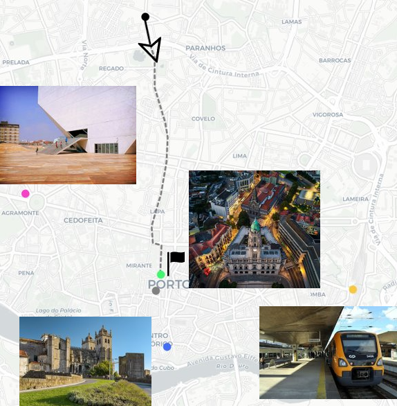
Figure 1. Where is the taxi passenger going? Based on only a few GPS points, the vehicle could be going to any number of locations, such as the Casa da Música perfomance center (west), the Sé do Porto cathedral (south), or the Estación de Porto-Campanhã train station (east), among others. In this case, the model’s prediction (gray) is very near the true destination, near the historic Câmara Municipal do Porto city hall. The current time might provide a hint about the passenger’s intentions, and different times of the day, week, or year might imply different destinations. (Photographs under CC BY 2.0, (Moratinos, 2005; Franganillo, 2017; Flickr user “Deensel” at https://www.flickr.com/people/158619309@N03, 2017; Miranda, 2014).)

Where is the taxi passenger going? Based on only a few GPS points, the vehicle could be going to any number of locations, such as the Casa da Música perfomance center (west), the Sé do Porto cathedral (south), or the Estación de Porto-Campanhã train station (east), among others. In this case, the model’s prediction (gray) is very near the true destination, near the historic Câmara Municipal do Porto city hall. The current time might provide a hint about the passenger’s intentions, and different times of the day, week, or year might imply different destinations.

1. Introduction

In recent years, the intersection of transportation and geospatial machine learning has expanded rapidly, fueled in part by a growing number of publicly available GPS datasets. Many are drawn from public transportation systems, especially taxicabs, which provide rich information about mobility patterns and behavior throughout a city while avoiding the privacy pitfall of publishing private vehicles’ trajectories. Common examples include taxis from San Francisco (Piorkowski et al., 2009), New York City (NYC Taxi & Limousine Commission, nd), Rome (Bracciale et al., 2014), and Beijing (Yuan et al., 2010). Perhaps the most well-known of these benchmarks is the Taxi Service Trajectory prediction challenge from ECML/PKDD 2015 (Geolink, 2015), which tracked 442 taxis in Porto, Portugal for one year. Competitors were challenged to predict a taxi’s final GPS destination given only a limited “prefix” of the first $n$ GPS points and limited metadata about the taxi ride (notably not including the total length). More than 380 teams participated in the competition, drawing research interest that continued even after its conclusion (Lv et al., 2018; Zhang et al., 2018; Rossi et al., 2019; Zhang et al., 2019; Li et al., 2020; Ebel et al., 2020; Liao et al., 2021; Tang et al., 2021; Tsiligkaridis et al., 2020). The Porto dataset has also contributed to other geospatial modeling interests, including passenger demand modeling (Moreira-Matias et al., 2013; Saadallah et al., 2018; Le Quy et al., 2019; Rodrigues et al., 2020), travel time prediction (Hoch, 2015; Gupta et al., 2018; Fu and Lee, 2019; Lan et al., 2019; Das et al., 2019; Abbar et al., 2020), and unsupervised geospatial learning and anomaly detection (Lam, 2016; Keane, 2017; Irvine et al., 2018; Song et al., 2018; Liu et al., 2020).

Given the successes modeling the primary GPS data, one might expect that the additional trajectory-level features, such as time, might also contain useful knowledge. For example, when modeling destinations, one might expect that Porto’s beaches would be busier in summer than winter; recreational areas, more popular on weekends; and restaurants and bars, more popular at mealtimes and evenings. Moreover, major holidays and events should exhibit learnable deviations from the typical patterns of everyday life. Instead, it is surprising how unuseful these metadata are, based on prior researchers’ ablation studies. For example, Ebel et al. (2020) found that these ancillary features reduced their mean error by merely 0.030 km, or roughly 2 percent of the GPS-only model’s error. In a second dataset from San Francisco, incorporating these metadata increased the average error between predicted and real destinations (Ebel et al., 2020).

In this work, we present a more powerful temporal prediction framework drawing on recent work in the meta-learning community. We show, by a series of careful experiments and ablations on the Porto dataset, that:

• Temporal cues do, in fact, improve performance on taxi destination prediction relative to a model without them, especially when few GPS points are available;

• A hypernetwork-based meta-learning framework outperforms the simple concatenatation of temporal and geospatial features commonly used in prior work;

• Different timescales (relative to the 24-hour, 7-day, and 1-year cycles) all contribute to this performance, and outperform a time-unaware baseline;

• Performance slightly, but noticeably, improves with later rather than earlier fusion. In other words, combining temporal and geospatial encodings works best in the model’s final layers, rather than its first ones.

2. Related Work

The task of destination and/or trajectory prediction is well-known in the domains of urban planning and management, intelligent transportation systems, “smart cities,” and ride-sharing applications, leading to a proliferation of research in the past few years (Altshuler et al., 2019; Anagnostopoulos, 2021; Zhao et al., 2019; Zheng et al., 2021; Xiao et al., 2020; Wang et al., 2020). Recent events have also energized a sub-field of mobility modeling and destination prediction for the purposes of pandemic analysis (Jiang et al., 2021). Many of these models fall broadly under the neural network framework, although they vary widely in their complexity. In the context of Porto, early successes were achieved by relatively simple multi-layer perceptron (MLP) models, such as the competition-winning result of De Brébisson et al. (2015), which outperformed competitors such as ensembles of regression trees (Lam et al., 2015). More recent papers have predominantly employed recurrent networks instead (Rossi et al., 2019; Liao et al., 2021; Li et al., 2020; Ebel et al., 2020; Zhang et al., 2018; Tang et al., 2021), particularly long short-term memory (LSTM) networks (Hochreiter and Schmidhuber, 1997). Notable exceptions include Lv et al. (2018), who plot trajectories graphically and then model them as 2D images rather than GPS points or embeddings, using convolutional networks, and Tsiligkaridis et al. (2020), who use Transformers (Vaswani et al., 2017).

Within the LSTM-based community, there remains significant diversity in the model architectures. Zhang et al. (2018) combine image-based CNN and GPS recurrent representations into a single predictive model. Ebel et al. (2020) and Liao et al. (2021) both perform a geospatial partitioning of the Porto area and train a LSTM over a sequence of region embeddings; Ebel et al. (2020) use $k$-d trees, while Liao et al. (2021) use grid-based and quadtree partitions and add an attention mechanism. In a unique approach, Rossi et al. (2019) consider a driver’s history rather than a passenger’s, modeling a sequence of pick-up/drop-off points across consecutive trajectories, rather than each trajectory individually. Our own approach is most closely related to Ebel et al. (2020) and Liao et al. (2021), in that we learn geospatial embeddings over GPS points and model trajectories as sequences of embeddings. However, the details of our approach, including our embedding mechanism, temporal representation, and model architecture, differ signficantly (see Sections 3.3, 3.4 and 4.1).

3. Methods

3.1. Problem Definition

3.1.1. Trajectory.

Let $\mathcal{T}$ be the set of all trajectories, where each trajectory $T:=((p_{i})^{N}_{i=1},M)$ is defined as a sequence of points $p_{1},\ldots,p_{N}$ where $N$ is the length of the trajectory and metadata $M$ associated with the trajectory. Each point $p_{i}=(\phi_{i},\lambda_{i})$ is an ordered pair of latitude and longitude values, and the destination of a trajectory is its final point $p_{N}$.

3.1.2. Trajectory prefix.

A partial trajectory, or trajectory fragment, is some contiguous sub-sequence of points $(p_{i})^{b}_{a}=p_{a},\ldots,p_{b}$ for some lower and upper indices $a,b$. We will refer to the $n$-length prefix of trajectory $T^{(n)}$ as the partial trajectory which starts at the beginning of the trajectory $p_{1}$ and is $n$ points long, where by assumption $1\leq n\leq N$.

3.1.3. Metadata.

The metadata $M$ are broadly defined as any additional information associated with a trajectory, such as an identifier for each taxi driver. Of particular interest is the timestamp $t$ (taken, in the Porto dataset, from the beginning of the trajectory). We hypothesize that the behavioral patterns of both drivers and passengers should vary with the time of day, day of the week, and season.

3.1.4. Haversine distance.

The Haversine distance measures the great-circle distance between two points on a sphere, i.e., the shortest distance between two points traveling along the sphere’s surface. Following the original competition metric, the distance between two points is

(1) $$d_{H}(p_{i},p_{j}) =2r\arctan\left(\sqrt{\frac{a}{1-a}}\right)\textrm{, with}$$

(2) $$a =\sin^{2}\left(\frac{\phi_{j}-\phi_{i}}{2}\right)+\cos\phi_{i}\cos\phi_{j}\sin^{2}\left(\frac{\lambda_{j}-\lambda_{i}}{2}\right)$$

Figure 2. Input encoding mechanism, converting GPS points to an embedding space. In contrast to prior work, we avoid performing a “hard assignment” or discrete partition of the geospatial area or road network. Instead, we learn embeddings for each of a set of 4,096 reference points, and each input point is encoded as a “soft” distance-weighted average of these embeddings.

3.1.5. Destination prediction

Our problem, then, is as follows: for any $n$, given a trajectory prefix $T^{(n)}=(p_{1},\ldots,p_{n})$ and metadata $M$, and predict the final destination $p_{N}$, such that the Haversine distance between the predicted and real $p_{N}$ is minimized. Notably, the prefix length $n$ is known but the length of the full trajectory $N$ is not, except that by definition $N\geq n$. In other words, the model must infer the final destination without being informed how much time or distance is remaining.

3.2. Data Preprocessing

For the purposes of fair comparison, we follow the preprocessing procedure outlined by Ebel et al. (2020):

1. We remove trajectories that are extremely short (2 minutes or less) or long (2 hours or longer), including those consisting of only a single data point.

2. If the apparent speed between two points is extremely large, we assume GPS measurement error. Whenever the speed greater than 240 km/h, we smooth the outliers with a median filter.

3. Any remaining trajectories which include points outside the Porto area are removed.

4. We remove roundtrips or sight-seeing trips, i.e., a long trajectory which starts and ends near the same point, traversing through points of interest, especially tourist ones. These trips only confound the problem of destination prediction. The roundtrip factor $\tau$ (Ebel et al., 2020) is the ratio of the trip’s total path length to the bee-line distance between its start and end. If $\tau$ is large, then the trajectory travels a long path but ends close to where it began.

   (3) $$\tau=\frac{\sum_{i}d_{H}(p_{i},p_{i+1})}{d_{H}(p_{1},p_{N})}$$

   Following Ebel et al. (2020), we only keep trajectories with $\tau<3.5$ (roughly the 95th percentile of $\tau$), and drop the remaining ones from the dataset.

3.3. Geospatial Encoding

Figure 3. Overall information flow of the model. A sequence of points is converted to a sequence of embeddings via a geospatial encoding mechanism (Section 3.3). This sequence is modeled by fully-connected and recurrent layers (Section 4.1), some parameterized by a hypernetwork (Section 3.5). The output is a softmax weight vector over the reference points from the geospatial encoding, which is simple to convert to a predicted point (Section 3.6). Thus, for every $i=1,\ldots,N$ we have a prediction $\hat{y}_{i}$ based on points $p_{1},\ldots,p_{i}$ trained to match the final destination $p_{N}$.

Most destination prediction models begin by partitioning the geospatial area into a set of regions. The ground-truth road network itself may be partitioned into segments (Neto et al., 2018; Lassoued et al., 2017; Li et al., 2016; Simmons et al., 2006). Alternatively, the geospatial area can be divided into uniform grids (Krumm and Horvitz, 2006; Manasseh and Sengupta, 2013; Endo et al., 2017; Pecher et al., 2016) or, with greater sophistication, into $k$-d tree-based regions so that smaller, more precise regions are used in areas with higher vehicle density (Xue et al., 2015; Ebel et al., 2020). (See (Ebel et al., 2020) for related discussion.) We instead propose an approach which does not explicitly partition the input GPS space at all (Fig. 2).

We randomly sample GPS points from training trajectories. At each random draw, we find the nearest neighbor in our current sample, and if this minimum distance is at least $d_{H}\geq 0.1$ km we add the point to our sample. We repeat until we have sampled $N_{ref}=4096$ points, which we refer to as the reference points, or $\tilde{p}$.

We instantiate an embedding table $\mathbf{E}_{ref}$ of shape $N_{ref}\times m$, that is, a table of $N_{ref}$ different embedding vectors of size $m$. These embeddings $\mathbf{E}_{ref}$ are learnable model parameters trained jointly with the rest of the model. To convert the points of a trajectory $T$ to embeddings, we consider each point $p_{i}=(\phi_{i},\lambda_{i})$ separately. We calculate the Haversine distance $d_{H}$ from $p_{i}$ to each reference point $\tilde{p}_{j}$. We then negate these distances and apply a softmax function, creating a $N_{ref}\times 1$ vector $\boldsymbol{\delta}$

(4) $$\delta_{j}=\frac{\exp(-d_{H}(p_{i},\tilde{p}_{j}))}{\sum_{k}\exp(-d_{H}(p_{i},\tilde{p}_{k}))}$$

so that $\delta_{j}$ is largest for reference points $\tilde{p}_{j}$ closest to the point $p_{i}$, and low for faraway points. Due to the softmax, $\boldsymbol{\delta}$ always sums to 1.

The embedding of point $p_{i}$ is an average of the embeddings of all the reference points, weighted by the proximity $\boldsymbol{\delta}$:

(5) $$e=\boldsymbol{\delta}^{\top}\mathbf{E}_{ref}$$

This converts the $N\times 2$ sequence of points into a $N\times m$ sequence of embeddings. We find that a relatively small embedding of size $m=16$ works well.

3.4. Temporal Encoding

We represent time as a set of continuous oscillating functions: the time of day, week, and year. Each takes the form of a sinusoidal embedding, which converts a timestamp (in hours) $t$ to a vector:

(6) $$c(t) =\sin\left(\frac{2\pi}{C}t+\boldsymbol{\varphi}\right)\mathrm{,with}$$

(7) $$\boldsymbol{\varphi} =\left[0,\frac{\pi}{2},\pi,\frac{3\pi}{2}\right]$$

where $C$ is the period in hours, i.e., 24, 168, and 8760 for a day, week, and year respectively.

3.4.1. Other metadata.

The Porto dataset also includes additional categorical metadata: (i) a unique ID anonymously identifying the customer’s phone number, if available, (ii) a unique ID identifying the taxi stand where the trip began, if applicable, and (iii) a unique ID for the taxi driver. We incorporate these metadata features as learned embeddings, as has long been popular for this dataset (De Brébisson et al., 2015), and concatenate them with the three temporal encodings $c(t)$.

Figure 4. Overall information flow of the model. A sequence of points is converted to a sequence of embeddings via a geospatial encoding mechanism (Section 3.3). This sequence is modeled by fully-connected and recurrent layers (Section 4.1), some parameterized by a hypernetwork (Section 3.5). The output is a softmax weight vector over the reference points from the geospatial encoding, which is simple to convert to a predicted point (Section 3.6). Thus, for every $i=1,\ldots,N$ we have a prediction $\hat{y}_{i}$ based on points $p_{1},\ldots,p_{i}$ trained to match the final destination $p_{N}$.

3.5. Hypernetwork and LSTM

Given a neural network $f_{\theta}(x)\rightarrow y$, that is, a network with weights $\theta$ trained to predict $y$ from $x$, a hypernetwork (Ha et al., 2017) refers to a network

(8) $$h_{\gamma}:Z\rightarrow\theta$$

which learns to generate the main network’s weights $\theta$ from some input $Z$. Because all operations in both $f$ and $h$ are differentiable, all learnable parameters can be trained via backpropagation. In practice, generating all parameters $\theta$ for an entire neural network is prohibitively expensive, and instead a subset of $\theta$ are generated by $h$. Recent authors have argued that this framing allows for a more powerful information fusion mechanism for two input streams in a neural network (Jayakumar et al., 2020; Galanti and Wolf, 2020) and suggest it as a drop-in replacement for concatenation. Outside the geospatial community, hypernetworks and related methods have found success in diverse applications including neural style transfer (Shen et al., 2018), time series analysis (Deng et al., 2020), multi-task (Mahabadi et al., 2021) and continual learning (von Oswald et al., 2020), robotic driving applications (Wang et al., 2018), reinforcement learning (Sarafian et al., 2021), and medical prediction (Ji and Marttinen, 2021). In our setting, we consider the case where the hypernetwork $h$ is a single fully-connected (linear) layer operating over the inputs described in Section 3.4, that is, $Z$ consists of the temporal encodings $c(t)$, the driver and customer ID, and the taxi stand if applicable. The architecture of the main network $f_{\theta}$ varies in our experiments (see Section 4.1) but may be a recurrent network, such as LSTM (Hochreiter and Schmidhuber, 1997), or another fully-connected layer.

The fully-connected layer, $\mathbf{W}\mathbf{x}+\mathbf{b}$, is the simpler case. Here, we simply have $\theta:=\{\mathbf{W},\mathbf{b}\}$, that is, we generate a weight matrix and bias vector from a hypernetwork $h_{\gamma}:Z\rightarrow\theta$. In our formulation, $\mathbf{W}$ and $\mathbf{b}$ are each generated by a fully-connected layer, so this hypernetwork $h$ is functionally equivalent to the multiplicative interaction discussed in detail by Jayakumar et al. (2020). The LSTM module (Hochreiter and Schmidhuber, 1997) internally can be viewed as four fully-connected layers (with appropriate non-linearities applied), so to paramaterize a LSTM via hypernetwork, we simply expand $\theta$ to generate four weight matrices and biases rather than one.

3.5.1. Weight Normalization

However, hypernetwork training can be difficult in practice; the optimization may be unstable, or may not converge at all. Hypernetworks, especially at initialization, often produce weights with substantially larger or smaller scales than necessary for training, leading to poor results. For specific model architectures, proper weight initialization schemes can be derived analytically (Chang et al., 2019), but they do not hold in general (e.g., for both linear and recurrent layers).

Similar to Krueger et al. (2017), we find that applying weight normalization (Salimans and Kingma, 2016) consistently succeeds in stabilizing the hypernetwork training process. For a weight vector $\mathbf{v}\in\theta$ generated by $h$, the normalized weight $\mathbf{w}$ is simply

(9) $$\mathbf{w}=\frac{g}{\|\mathbf{v}\|}\mathbf{v}$$

where $g$ is a scalar learned via backpropagation. The generated weight $\mathbf{v}$ is normalized and multiplied by this learned constant, guaranteeing that the scale of $\mathbf{w}$ is always $g$. In other words, the hypernetwork generates the direction of this vector, but not its scale. Since generating weights on the wrong scale is the cause of poor training in the first place, this simple reparameterization trick resolves any instability in training and enables us to train hypernetworks $h$ for both fully-connected and LSTM networks $f$ without further interventions, such as custom weight initialization schemes.

(a) Pre-LSTM hypernetwork.

(b) Hyper-LSTM.

(c) Post-LSTM hypernetwork.

Figure 5. Fusion may occur before the recurrent network, altering the geospatial embeddings 5(a); in the recurrent network itself, changing the LSTM weights 5(b); or after the LSTM entirely 5(c). Hypernetwork ($h$) and model layers parameterized by it ($f$) highlighted in green.

3.6. GPS Output Layer

We follow a standard approach for this problem (including the original competition winner (De Brébisson et al., 2015)): a softmax final layer generating a weight vector of a set of predefined points (which we call $\boldsymbol{\alpha}$). The final GPS vector is then a weighted average of the points,

(10) $$\hat{y}=\sum_{j}\alpha_{j}\tilde{p}_{j}$$

Note that these points $\tilde{p}$ are the same reference points used in Section 3.3 for the model’s input. Thus $\tilde{p}$ are used to transform GPS points both to and from higher-dimensional embedding spaces used internally by the model, and $\boldsymbol{\alpha}$ serves a similar role to $\boldsymbol{\delta}$ (Section 3.3), both softmax weight vectors over these reference points.

Note that for every point $p_{i}\in T$, we have a predicted destination $\hat{y}_{i}$ predicted from $p_{1},\ldots,p_{i}$. The training loss for a given trajectory $T$ is simply the mean Haversine distance between these predictions and the true destination $p_{N}$:

(11) $$\mathcal{L}(\hat{y},p_{N})=\frac{1}{N}\sum_{i=1}^{N}d_{H}(\hat{y}_{i},p_{N})$$

The evaluation metric is the Mean Haversine Distance (MHD), or the quantity in Eq. 11 averaged over all trajectories in the validation set (a random sample of 10,000 trajectories held out from training). All models are trained for 10 epochs.

Following prior work, we will also consider the MHD over particular prefix lengths. For example, $MHD_{0.1}$ is the Haversine distance $d_{H}(\hat{y}_{i},p_{N})$ when $i$ corresponds to the first 10 percent of a trajectory, averaged over the validation set of trajectories.

4. Experimental Results

Model	$MHD$	$MHD_{0.1}$	$MHD_{0.3}$	$MHD_{0.5}$	$MHD_{0.7}$	$MHD_{0.9}$
Results reported by prior work
Liao et al. (2021)*$\dagger$	1.481	2.848	2.175	1.254	0.560	0.572
Ebel et al. (2020)	1.460	2.71$\ddagger$	1.97$\ddagger$	1.26$\ddagger$	0.84$\ddagger$	0.69$\ddagger$
Ebel et al. (2020)*	1.430	2.69$\ddagger$	1.93$\ddagger$	1.237	0.82$\ddagger$	0.66$\ddagger$
Our results
pre-LSTM	1.354	2.482	1.844	1.225	0.729	0.394
hyper-LSTM	1.320	2.459	1.825	1.214	0.691	0.334
post-LSTM	1.317	2.429	1.800	1.195	0.678	0.335

Table 1. Our results relative to previously published ones. All results in kilometers (km). Best result in bold and second-best in italics. See Section 4.1. *: This result includes additional data added to the Porto dataset (e.g., weather (Ebel et al., 2020), road network (Liao et al., 2021)). $\dagger$: Included due to similar methods and results to (Ebel et al., 2020), but note subtle differences in preprocessing. $\ddagger$: Approximated from published graphical results.

Model	$MHD$
Full model (post-LSTM, Table 1)	1.317
Remove hypernetwork (Section 4.2.1)
Concatenation	1.432
No metadata	1.382
Single timescales (Section 4.2.2)
Day only	1.322
Week only	1.329
Year only	1.337

Table 2. Ablations of the best-performing hypernetwork. All results in kilometers (km). See Section 4.2.

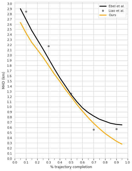
Figure 6. Comparison of the mean Haversine distance (MHD) of our best-performing model (post-LSTM; Fig. 5(c)) vs two strong published results (Ebel et al. (2020) and Liao et al. (2021)). Lower MHD denotes better performance. See also Table 1.

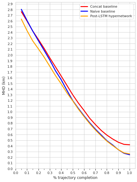
Figure 7. Ablation of our hypernetwork. The superior performance (lower MHD) of the hypernetwork (see Table 2) seems especially concentrated in the first half of the trajectory. When most of the trajectory points have been provided, a simple LSTM without metadata is competitive; however, when few GPS points are provided, the hypernetwork significantly outperforms both alternatives.

4.1. Model comparison

Despite the Porto dataset’s original use as a standardized benchmark for open competition, design choices in subsequent work make cross-paper comparison difficult. Firstly, different papers often augment the dataset with their own metadata not present in the original release, which may give some models an advantage over others independent of architecture or training design. For example, Rossi et al. (2019) incorporate point-of-interest (POI) data from Foursquare; Liao et al. (2021) include road networks from OpenStreetMap; Ebel et al. (2020) train with (and without) additional weather data. Additionally, different teams have used different preprocessing pipelines, with potentially significant deviations in the resulting training (and validation) data. Particularly problematic is the removal or alteration of “difficult” trajectories, such as those with GPS measurement error or destinations far outside Porto. With roughly 1.7 million trajectories to begin, Liao et al. (2021) “select the data located in the main areas of the city,” resulting in 665,989 trajectories; Ebel et al. (2020) delete trips outside the Porto area and maintain 1,545,240 trajectories. Other rule-out criteria include trajectory length (e.g., (Ebel et al., 2020; Zhang et al., 2018)) or missing GPS points, detected due to large instantaneous speed between two points (e.g., (Lam et al., 2015; Ebel et al., 2020)). Taken together, all these steps have the effect of removing the most difficult-to-predict trajectories from training and validation, biasing any evaluation against other papers’ published metrics.

Given these limitations, Ebel et al. (2020)’s result (without weather added) is, to our knowledge, the best published performance of any model without substantial additional metadata. We therefore take this as our baseline, and re-implement its preprocessing pipeline, validation split, etc. for fair comparison. We note, however, that the more recent results of Liao et al. (2021) are numerically similar to those of Ebel et al. (2020) despite the addition of a road network and more aggressive subsampling of the trajectories during preprocessing. We outperform both methods, and both methods in turn outperform their authors’ custom baselines and the original competition winner (De Brébisson et al., 2015).

Because hypernetworks have not been applied to this problem before, we investigate the optimal stage of fusing metadata (including time) with the recurrent model. A hypernetwork can be used to parameterize the weights at any arbitrary layer of the model (Fig. 5). We compare three possibilities (Fig. 5):

1. The hypernetwork $h$ parameterizes a linear layer placed before the LSTM (Fig. 5(a)). We call this the “pre-LSTM” model.

2. The hypernetwork $h$ parameterizes all weights of the LSTM itself (Fig. 5(b)). We call this the “hyper-LSTM” model.

3. The hypernetwork $h$ parameterizes a linear layer placed after the LSTM (Fig. 5(c)). We call this the “post-LSTM” model.

We show the results, relative to Ebel et al. (2020) and Liao et al. (2021), in Tables 1 and 6.

Comparing the two prior publications, we see that despite similar $MHD$ values overall, Ebel et al. (2020)’s method tends to perform better early in the trajectory and Liao et al. (2021) performs better late. This is perhaps because Liao et al. (2021) train only on prefixes of length 70%, as opposed to varying lengths, allowing the model to specialize in late-trajectory prediction. Note that Liao et al. (2021)’s error increases when more of the trajectory, 90%, is provided, suggesting the model’s preference for 70% prefixes.

Our proposed methods consistently outperform both methods in both the primary competition metric $MHD$ (Table 1) and most prefix lengths individually (Tables 1 and 6), with Liao et al. (2021) at 70% the only exception. In the first third of the trajectory, our method cleanly outperforms both prior papers. In the middle, all three methods are competitive, although ours remains narrowly better (by about 0.05 km). In the final third, Ebel et al. (2020) and Liao et al. (2021) plateau around 0.66 and 0.56 km respectively, while our method continues to sharply reduce its error as more GPS points are provided, achieving errors below 0.3 km.

We also see that later fusion generally outperforms early fusion, and in particular placing the hypernetwork prior to the LSTM leads to weaker performance (Table 1), while the other two methods (hyper- and post-LSTM) are competitive. However, all three hypernetworks outperform the prior state-of-the-art method, even without additional data such as weather conditions (Ebel et al., 2020) or a ground-truth road network (Liao et al., 2021).

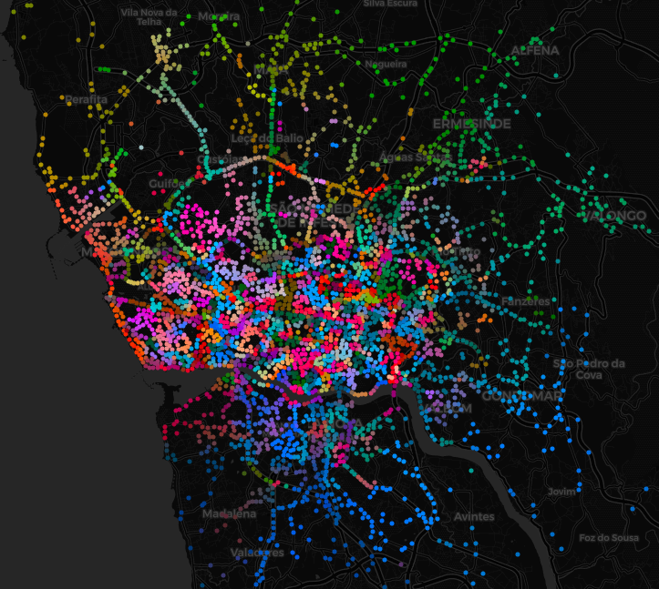
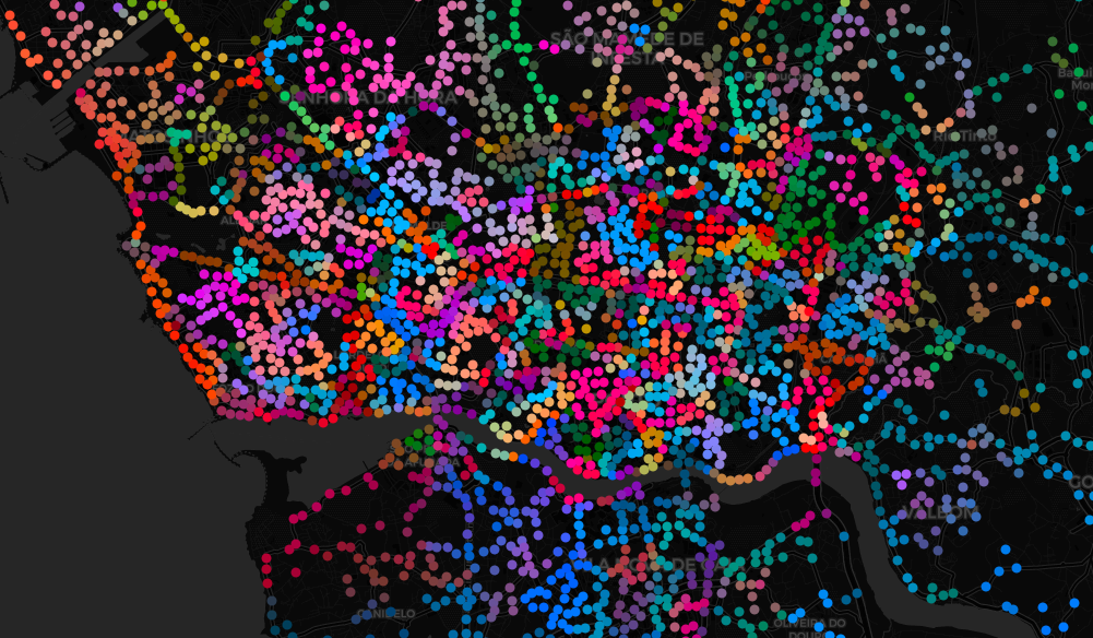
Figure 8. Visualizing embeddings of the Porto reference points. Left, the larger Porto area; right, focused on the downtown area. The model naturally learns an apparent unsupervised segmentation of the geospatial area with strong spatial locality. North of the city, highways are segmented into distinct colors near major turns or exits; in the west, beaches are a consistent color (reddish-orange) interrupted only by the historic site Castelo do Queijo (gray); downtown, the city appears to be grouped into distinct neighborhoods and districts with variable sizes and shapes and distinct borders. Best viewed in color.

4.2. Ablations

4.2.1. Hypernetwork versus alternatives.

In addition to the numeric results reported by prior work, we also implement custom baselines which do not use hypernetworks. This ensures that unique aspects of our approach, such as the geospatial encoding (Section 3.3) and model hyperparameters (e.g., layer sizes) remain constant, quantifying the exact contribution of the hypernetwork. We consider two models:

1. A model which concatenates the metadata with the main geospatial features after the LSTM (similar to Ebel et al. (2020) and Liao et al. (2021), among many others) then passes them through a fully-connected layer. We refer to this as the “concatenation baseline.”

2. A model which does not use the metadata at all. We refer to this as the “naïve baseline.”

Both ablations underperform our main model (Table 2). Removing the hypernetwork and replacing it with prior approaches degrades model performance.

Fig. 7 further illustrates the circumstances under which our hypernetwork improves upon more common approaches. In the first half of the trajectory, the hypernetwork outperforms both the ablations by a significant margin (concatenation: 129 meters; naïve: 171 meters). However, in the second half (when a majority of the trajectory points are visible to the model) the naïve baseline becomes competitive: the geospatial information alone is sufficient for the prediction. Thus, the hypernetwork’s improved performance draws from the most difficult cases, where few points have been provided and they are inadequate to predict the final destination alone, as we hypothesized in Fig. 1.

4.2.2. Different components of time.

Recall from Section 3.4 that we model time as sinusoids of period 1 day, 1 week, and 1 year. To evaluate each timescale’s contribution, we modify the best-performing model (Table 1) to produce three more models. Each ablated model receives only one timescale—either day, week, or year—in addition to the remaining metadata.

We can see in Table 2 that all three ablations perform slightly worse than the full model, but better than the concatenation or naïve baselines. We therefore conclude that all three timescales—daily, weekly, and yearly patterns—contribute in some degree to the model’s performance.

4.3. Visualizing the region encodings

Finally, we qualitatively investigate the geospatial encoding proposed in Section 3.3. Recall that each of the $N_{ref}=4096$ reference points is associated with a learned embedding vector of size $m=16$. We employ t-SNE (Van der Maaten and Hinton, 2008) to reduce these embedding vectors into a 3D space, which we then rescale and interpret as color values. This allows us to map all embedding vectors to colors; we can then plot the GPS reference points (as originally shown in Fig. 2), but now color-coded by their embeddings to inspect them for structure.

The results of this visualization are shown in Fig. 8. Compared to prior works that impose uniform grids, manual road network segmentations, $k$-d or quadtrees, etc., our results show a categorically better expression of Porto’s geospatial structure. The t-SNE dimensionality reduction operates on the embedding vectors, not the GPS values, but the embeddings still display strong geospatial locality. The embeddings appear to segment Porto into distinct learned regions. In the north outside the main city, where GPS points are sparse, highways are split into segments near major turns and exits. In contrast, the denser downtown area appears grouped into neighborhoods and districts of variable size and shape. In a unique example, Porto’s beaches (the western edge of the city) all take a similar reddish-orange embedding, with a small brownish-gray subregion around the Castelo do Queijo, a historic seaside fortress and major landmark. We can also see evidence in some locations of “blending” or interpolation for points between districts.

This structure is learned entirely without additional supervision, simply as a means to achieve the model’s primary task of destination prediction. Its adaptability to, and expressiveness of, Porto’s geospatial structure cannot be matched by recently published state-of-the-art, which simply assigns input points to variably-sized rectangles from $k$-d trees (Ebel et al., 2020) or uniform grids and variably-sized squares from quadtrees (Liao et al., 2021).

5. Conclusion

We propose a model for destination prediction tasks which incorporates novel geospatial and temporal representations, and we validate them by achieving state-of-the-art performance on the Porto dataset. Our thorough ablation experiments confirm that our hypernetwork outperforms a concatenation-based approach common in prior work, and that different timescales each play a role in the improving the model’s performance. We anticipate that improved prediction of vehicle destinations will be useful in urban planning, ride-sharing, and intelligent transportation applications.

- (1)
- Abbar et al. (2020) Sofiane Abbar, Rade Stanojevic, and Mohamed Mokbel. 2020. STAD: Spatio-temporal adjustment of traffic-oblivious travel-time estimation. In 2020 21st IEEE International Conference on Mobile Data Management (MDM). IEEE, 79–88.
- Altshuler et al. (2019) Tal Altshuler, Yaniv Altshuler, Rachel Katoshevski, and Yoram Shiftan. 2019. Modeling and prediction of ride-sharing utilization dynamics. Journal of Advanced Transportation 2019 (2019).
- Anagnostopoulos (2021) Theodoros Anagnostopoulos. 2021. A Predictive Vehicle Ride Sharing Recommendation System for Smart Cities Commuting. Smart Cities 4, 1 (2021), 177–191.
- Bracciale et al. (2014) Lorenzo Bracciale, Marco Bonola, Pierpaolo Loreti, Giuseppe Bianchi, Raul Amici, and Antonello Rabuffi. 2014. CRAWDAD dataset roma/taxi (v. 2014-07-17). Downloaded from https://crawdad.org/roma/taxi/20140717. https://doi.org/10.15783/C7QC7M
- Chang et al. (2019) Oscar Chang, Lampros Flokas, and Hod Lipson. 2019. Principled weight initialization for hypernetworks. In International Conference on Learning Representations.
- Das et al. (2019) Soumi Das, Rajath Nandan Kalava, Kolli Kiran Kumar, Akhil Kandregula, Kalpam Suhaas, Sourangshu Bhattacharya, and Niloy Ganguly. 2019. Map enhanced route travel time prediction using deep neural networks. arXiv preprint arXiv:1911.02623 (2019).
- De Brébisson et al. (2015) Alexandre De Brébisson, Étienne Simon, Alex Auvolat, Pascal Vincent, and Yoshua Bengio. 2015. Artificial neural networks applied to taxi destination prediction. In Proceedings of the 2015th International Conference on ECML PKDD Discovery Challenge-Volume 1526. 40–51.
- Deng et al. (2020) Ruizhi Deng, Yanshuai Cao, Bo Chang, Leonid Sigal, Greg Mori, and Marcus A Brubaker. 2020. Variational Hyper RNN for Sequence Modeling. arXiv preprint arXiv:2002.10501 (2020).
- Ebel et al. (2020) Patrick Ebel, Ibrahim Emre Göl, Christoph Lingenfelder, and Andreas Vogelsang. 2020. Destination prediction based on partial trajectory data. In 2020 IEEE Intelligent Vehicles Symposium (IV). IEEE, 1149–1155.
- Endo et al. (2017) Yuki Endo, Kyosuke Nishida, Hiroyuki Toda, and Hiroshi Sawada. 2017. Predicting destinations from partial trajectories using recurrent neural network. In Pacific-Asia Conference on Knowledge Discovery and Data Mining. Springer, 160–172.
- Flickr user “Deensel” at https://www.flickr.com/people/158619309@N03 (2017) Flickr user “Deensel” at https://www.flickr.com/people/158619309@N03. 2017. Porto City Hall. https://www.flickr.com/photos/deensel/36248265634/ under Creative Commons Attribution 2.0 Generic License (CC BY 2.0).
- Franganillo (2017) Jorge Franganillo. 2017. Porto: Sè do Porto. https://www.flickr.com/photos/franganillo/36934656926/ under Creative Commons Attribution 2.0 Generic License (CC BY 2.0).
- Fu and Lee (2019) Tao-yang Fu and Wang-Chien Lee. 2019. DeepIST: Deep image-based spatio-temporal network for travel time estimation. In Proceedings of the 28th ACM International Conference on Information and Knowledge Management. 69–78.
- Galanti and Wolf (2020) Tomer Galanti and Lior Wolf. 2020. On the modularity of hypernetworks. Advances in Neural Information Processing Systems 33 (2020).
- Geolink (2015) Geolink. 2015. Taxi Service Trajectory (TST) Prediction Challenge @ ECML/PKDD 2015. https://web.archive.org/web/20150715062001/http://www.geolink.pt/ecmlpkdd2015-challenge/dataset.html.
- Gupta et al. (2018) Bharat Gupta, Shivam Awasthi, Rudraksha Gupta, Likhama Ram, Pramod Kumar, Bakshi Rohit Prasad, and Sonali Agarwal. 2018. Taxi travel time prediction using ensemble-based random forest and gradient boosting model. In Advances in Big Data and Cloud Computing. Springer, 63–78.
- Ha et al. (2017) David Ha, Andrew Dai, and Quoc V Le. 2017. Hypernetworks. International Conference of Learning Representations (2017).
- Hoch (2015) Thomas Hoch. 2015. An Ensemble Learning Approach for the Kaggle Taxi Travel Time Prediction Challenge.. In DC@ PKDD/ECML.
- Hochreiter and Schmidhuber (1997) Sepp Hochreiter and Jürgen Schmidhuber. 1997. Long short-term memory. Neural computation 9, 8 (1997), 1735–1780.
- Irvine et al. (2018) John M Irvine, Laura Mariano, and Teal Guidici. 2018. Normalcy modeling using a dictionary of activities learned from motion imagery tracking data. In 2018 IEEE Applied Imagery Pattern Recognition Workshop (AIPR). IEEE, 1–9.
- Jayakumar et al. (2020) Siddhant M Jayakumar, Wojciech M Czarnecki, Jacob Menick, Jonathan Schwarz, Jack Rae, Simon Osindero, Yee Whye Teh, Tim Harley, and Razvan Pascanu. 2020. Multiplicative interactions and where to find them. In International Conference on Learning Representations.
- Ji and Marttinen (2021) Shaoxiong Ji and Pekka Marttinen. 2021. Patient Outcome and Zero-shot Diagnosis Prediction with Hypernetwork-guided Multitask Learning. arXiv preprint arXiv:2109.03062 (2021).
- Jiang et al. (2021) Renhe Jiang, Zhaonan Wang, Zekun Cai, Chuang Yang, Zipei Fan, Tianqi Xia, Go Matsubara, Hiroto Mizuseki, Xuan Song, and Ryosuke Shibasaki. 2021. Countrywide Origin-Destination Matrix Prediction and Its Application for COVID-19. In Joint European Conference on Machine Learning and Knowledge Discovery in Databases. Springer, 319–334.
- Keane (2017) Kevin R Keane. 2017. Detecting motion anomalies. In Proceedings of the 8th ACM SIGSPATIAL Workshop on GeoStreaming. 21–28.
- Krueger et al. (2017) David Krueger, Chin-Wei Huang, Riashat Islam, Ryan Turner, Alexandre Lacoste, and Aaron Courville. 2017. Bayesian hypernetworks. arXiv preprint arXiv:1710.04759 (2017).
- Krumm and Horvitz (2006) John Krumm and Eric Horvitz. 2006. Predestination: Inferring destinations from partial trajectories. In International Conference on Ubiquitous Computing. Springer, 243–260.
- Lam (2016) Hoang Thanh Lam. 2016. A concise summary of spatial anomalies and its application in efficient real-time driving behaviour monitoring. In Proceedings of the 24th ACM SIGSPATIAL International Conference on Advances in Geographic Information Systems. 1–9.
- Lam et al. (2015) Hoang Thanh Lam, Ernesto Diaz-Aviles, Alessandra Pascale, Yiannis Gkoufas, and Bei Chen. 2015. (Blue) taxi destination and trip time prediction from partial trajectories. In Proceedings of the 2015th International Conference on ECML PKDD Discovery Challenge-Volume 1526. 63–74.
- Lan et al. (2019) Wuwei Lan, Yanyan Xu, and Bin Zhao. 2019. Travel time estimation without road networks: an urban morphological layout representation approach. In Proceedings of the 28th International Joint Conference on Artificial Intelligence. 1772–1778.
- Lassoued et al. (2017) Yassine Lassoued, Julien Monteil, Yingqi Gu, Giovanni Russo, Robert Shorten, and Martin Mevissen. 2017. A hidden Markov model for route and destination prediction. In 2017 IEEE 20th International Conference on Intelligent Transportation Systems (ITSC). IEEE, 1–6.
- Le Quy et al. (2019) Tai Le Quy, Wolfgang Nejdl, Myra Spiliopoulou, and Eirini Ntoutsi. 2019. A neighborhood-augmented LSTM model for taxi-passenger demand prediction. In International Workshop on Multiple-Aspect Analysis of Semantic Trajectories. Springer, 100–116.
- Li et al. (2016) Xiang Li, Mengting Li, Yue-Jiao Gong, Xing-Lin Zhang, and Jian Yin. 2016. T-DesP: Destination prediction based on big trajectory data. IEEE Transactions on Intelligent Transportation Systems 17, 8 (2016), 2344–2354.
- Li et al. (2020) Yadong Li, Bailong Liu, Lei Zhang, Susong Yang, Changxing Shao, and Dan Son. 2020. Fast Trajectory Prediction Method With Attention Enhanced SRU. IEEE Access 8 (2020), 206614–206621.
- Liao et al. (2021) Chengwu Liao, Chao Chen, Chaocan Xiang, Hongyu Huang, Hong Xie, and Songtao Guo. 2021. Taxi-Passenger’s Destination Prediction via GPS Embedding and Attention-Based BiLSTM Model. IEEE Transactions on Intelligent Transportation Systems (2021).
- Liu et al. (2020) Yiding Liu, Kaiqi Zhao, Gao Cong, and Zhifeng Bao. 2020. Online anomalous trajectory detection with deep generative sequence modeling. In 2020 IEEE 36th International Conference on Data Engineering (ICDE). IEEE, 949–960.
- Lv et al. (2018) Jianming Lv, Qing Li, Qinghui Sun, and Xintong Wang. 2018. T-CONV: A convolutional neural network for multi-scale taxi trajectory prediction. In 2018 IEEE international conference on big data and smart computing (bigcomp). IEEE, 82–89.
- Mahabadi et al. (2021) Rabeeh Karimi Mahabadi, Sebastian Ruder, Mostafa Dehghani, and James Henderson. 2021. Parameter-efficient multi-task fine-tuning for transformers via shared hypernetworks. arXiv preprint arXiv:2106.04489 (2021).
- Manasseh and Sengupta (2013) Christian Manasseh and Raja Sengupta. 2013. Predicting driver destination using machine learning techniques. In 16th International IEEE Conference on Intelligent Transportation Systems (ITSC 2013). IEEE, 142–147.
- Miranda (2014) Tiago Miranda. 2014. CP 3400 - Porto Campanhã. https://www.flickr.com/photos/tiago_miranda94/14277888315/ under Creative Commons Attribution 2.0 Generic License (CC BY 2.0).
- Moratinos (2005) Eduardo Moratinos. 2005. Casa da musica - llegaron los marcianos. https://commons.wikimedia.org/wiki/File:Casa_da_Musica_3_(Porto).jpg under Creative Commons Attribution 2.0 Generic License (CC BY 2.0).
- Moreira-Matias et al. (2013) Luis Moreira-Matias, Joao Gama, Michel Ferreira, Joao Mendes-Moreira, and Luis Damas. 2013. Predicting taxi–passenger demand using streaming data. IEEE Transactions on Intelligent Transportation Systems 14, 3 (2013), 1393–1402.
- Neto et al. (2018) Francisco Dantas Nobre Neto, Cláudio de Souza Baptista, and Claudio EC Campelo. 2018. Combining Markov model and prediction by partial matching compression technique for route and destination prediction. Knowledge-Based Systems 154 (2018), 81–92.
- NYC Taxi & Limousine Commission (nd) NYC Taxi & Limousine Commission. n.d.. TLC Trip Record Data. https://www1.nyc.gov/site/tlc/about/tlc-trip-record-data.page.
- Pecher et al. (2016) Philip Pecher, Michael Hunter, and Richard Fujimoto. 2016. Data-driven vehicle trajectory prediction. In Proceedings of the 2016 ACM SIGSIM Conference on Principles of Advanced Discrete Simulation. 13–22.
- Piorkowski et al. (2009) Michal Piorkowski, Natasa Sarafijanovic-Djukic, and Matthias Grossglauser. 2009. CRAWDAD dataset epfl/mobility (v. 2009-02-24). Downloaded from https://crawdad.org/epfl/mobility/20090224. https://doi.org/10.15783/C7J010
- Rodrigues et al. (2020) Pedro Rodrigues, Ana Martins, Sofia Kalakou, and Filipe Moura. 2020. Spatiotemporal variation of taxi demand. Transportation Research Procedia 47 (2020), 664–671.
- Rossi et al. (2019) Alberto Rossi, Gianni Barlacchi, Monica Bianchini, and Bruno Lepri. 2019. Modelling taxi drivers’ behaviour for the next destination prediction. IEEE Transactions on Intelligent Transportation Systems 21, 7 (2019), 2980–2989.
- Saadallah et al. (2018) Amal Saadallah, Luis Moreira-Matias, Ricardo Sousa, Jihed Khiari, Erik Jenelius, and Joao Gama. 2018. BRIGHT—drift-aware demand predictions for taxi networks. IEEE Transactions on Knowledge and Data Engineering 32, 2 (2018), 234–245.
- Salimans and Kingma (2016) Tim Salimans and Durk P Kingma. 2016. Weight normalization: A simple reparameterization to accelerate training of deep neural networks. Advances in neural information processing systems 29 (2016).
- Sarafian et al. (2021) Elad Sarafian, Shai Keynan, and Sarit Kraus. 2021. Recomposing the Reinforcement Learning Building Blocks with Hypernetworks. In International Conference on Machine Learning. PMLR, 9301–9312.
- Shen et al. (2018) Falong Shen, Shuicheng Yan, and Gang Zeng. 2018. Neural style transfer via meta networks. In Proceedings of the IEEE Conference on Computer Vision and Pattern Recognition. 8061–8069.
- Simmons et al. (2006) Reid Simmons, Brett Browning, Yilu Zhang, and Varsha Sadekar. 2006. Learning to predict driver route and destination intent. In 2006 IEEE Intelligent Transportation Systems Conference. IEEE, 127–132.
- Song et al. (2018) Li Song, Ruijia Wang, Ding Xiao, Xiaotian Han, Yanan Cai, and Chuan Shi. 2018. Anomalous trajectory detection using recurrent neural network. In International Conference on Advanced Data Mining and Applications. Springer, 263–277.
- Tang et al. (2021) Jinjun Tang, Jian Liang, Tianjian Yu, Yong Xiong, and Guoliang Zeng. 2021. Trip destination prediction based on a deep integration network by fusing multiple features from taxi trajectories. IET Intelligent Transport Systems 15, 9 (2021), 1131–1141.
- Tsiligkaridis et al. (2020) Athanasios Tsiligkaridis, Jing Zhang, Hiroshi Taguchi, and Daniel Nikovski. 2020. Personalized destination prediction using transformers in a contextless data setting. In 2020 International Joint Conference on Neural Networks (IJCNN). IEEE, 1–7.
- Van der Maaten and Hinton (2008) Laurens Van der Maaten and Geoffrey Hinton. 2008. Visualizing data using t-SNE. Journal of machine learning research 9, 11 (2008).
- Vaswani et al. (2017) Ashish Vaswani, Noam Shazeer, Niki Parmar, Jakob Uszkoreit, Llion Jones, Aidan N Gomez, Łukasz Kaiser, and Illia Polosukhin. 2017. Attention is all you need. Advances in neural information processing systems 30 (2017).
- von Oswald et al. (2020) Johannes von Oswald, Christian Henning, João Sacramento, and Benjamin F Grewe. 2020. Continual learning with hypernetworks. International Conference on Learning Representations (2020).
- Wang et al. (2018) Ruohan Wang, Pierluigi V Amadori, and Yiannis Demiris. 2018. Real-time workload classification during driving using hypernetworks. In 2018 IEEE/RSJ International Conference on Intelligent Robots and Systems (IROS). IEEE, 3060–3065.
- Wang et al. (2020) Wei Wang, Xiaofeng Zhao, Zhiguo Gong, Zhikui Chen, Ning Zhang, and Wei Wei. 2020. An attention-based deep learning framework for trip destination prediction of sharing bike. IEEE Transactions on Intelligent Transportation Systems 22, 7 (2020), 4601–4610.
- Xiao et al. (2020) Zhu Xiao, Shenyuan Xu, Tao Li, Hongbo Jiang, Rui Zhang, Amelia C Regan, and Hongyang Chen. 2020. On extracting regular travel behavior of private cars based on trajectory data analysis. IEEE Transactions on Vehicular Technology 69, 12 (2020), 14537–14549.
- Xue et al. (2015) Andy Yuan Xue, Jianzhong Qi, Xing Xie, Rui Zhang, Jin Huang, and Yuan Li. 2015. Solving the data sparsity problem in destination prediction. The VLDB Journal 24, 2 (2015), 219–243.
- Yuan et al. (2010) Jing Yuan, Yu Zheng, Chengyang Zhang, Wenlei Xie, Xing Xie, Guangzhong Sun, and Yan Huang. 2010. T-Drive: Driving Directions Based on Taxi Trajectories. In Proceedings of 18th ACM SIGSPATIAL Conference on Advances in Geographical Information Systems (proceedings of 18th acm sigspatial conference on advances in geographical information systems ed.). ACM SIGSPATIAL GIS 2010. https://www.microsoft.com/en-us/research/publication/t-drive-driving-directions-based-on-taxi-trajectories/ Best Paper Award.
- Zhang et al. (2018) Lei Zhang, Guoxing Zhang, Zhizheng Liang, and Ekene Frank Ozioko. 2018. Multi-features taxi destination prediction with frequency domain processing. PloS one 13, 3 (2018), e0194629.
- Zhang et al. (2019) Xiaocai Zhang, Zhixun Zhao, Yi Zheng, and Jinyan Li. 2019. Prediction of taxi destinations using a novel data embedding method and ensemble learning. IEEE Transactions on Intelligent Transportation Systems 21, 1 (2019), 68–78.
- Zhao et al. (2019) Bing Zhao, Yon Shin Teo, Wee Siong Ng, and Hai Heng Ng. 2019. Data-driven next destination prediction and ETA improvement for urban delivery fleets. IET Intelligent Transport Systems 13, 11 (2019), 1624–1635.
- Zheng et al. (2021) Guanjie Zheng, Chang Liu, Hua Wei, Chacha Chen, and Zhenhui Li. 2021. Rebuilding city-wide traffic origin destination from road speed data. In 2021 IEEE 37th International Conference on Data Engineering (ICDE). IEEE, 301–312.