A numerically robust, parallel-friendly variant of BiCGSTAB for the semi-implicit integration of the viscous term in Smoothed Particle Hydrodynamics

Abstract

Implicit integration of the viscous term can significantly improve performance in computational fluid dynamics for highly viscous fluids such as lava. We show improvements over our previous proposal for semi-implicit viscous integration in Smoothed Particle Hydrodynamics, extending it to support a wider range of boundary models. Due to the resulting loss of matrix symmetry, a key advancement is a more robust version of the biconjugate gradient stabilized method to solve the linear systems, that is also better suited for parallelization in both shared-memory and distributed-memory systems. The advantages of the new solver are demostrated in applications with both Newtonian and non-Newtonian fluids, covering both the numerical aspect (improved convergence thanks to the possibility to use more accurate boundary model) and the computing aspect (with excellent strong scaling and satisfactory weak scaling).

1 Introduction

Smoothed Particle Hydrodynamics (SPH) is a Lagrangian, mesh-free numerical method for computational fluid dynamics originally designed for astrophysics [1, 2] that has since been adopted in contexts spanning from oceanography to geophysics and industrial applications [3, 4, 5].

For liquids, the SPH numerical method is usually associated with a weakly compressible formulation (WCSPH), so that the system of Navier–Stokes and mass conservation equations is closed by introducing an equation of state that allows direct computation of the pressure from the other state variables (usually just the density), but density variations are kept small enough (in the order of $1\%$) to be considered negligible [6].

A significant computational benefit of the standard WCSPH formulations, when paired with an explicit integration scheme, is that the method becomes trivially parallelizable, and can easily take advantage of high-performance parallel computing hardware [7].

The GPUSPH particle engine [8] was the first implementation of WCSPH to run entirely on Graphics Processing Units (GPUs) using CUDA, leveraging the ease of parallelization to achieve significant speed-ups over equivalent serial code. Originally limited to single-GPU simulations of Newtonian fluids, GPUSPH has since been extended with the aim of becoming a high-performance, numerically robust and physically accurate simulation engine for complex fluids: it now allows the distribution of computation across multiple GPUs on the same machine [9] as well as across GPU-equipped nodes in a cluster [10], and it covers a wider range of physical models, including support for non-Newtonian rheologies and thermo-dynamics, with the specific intent of becoming an essential tool for the study of lava flows [11, 12, 13].

The downside of adopting an explicit integration scheme is the potentially small time-step, constrained by CFL-like conditions for the sound speed, maximum forces magnitude, and diffusive coefficients (kinematic viscosity, thermal diffusitivity, etc). In particular, for simulations with a very low Reynolds number, the dominant factor in the time-step for explicitly integrated WCSPH is given by the viscous contribution. To work around this issue, several alternatives have been proposed, centered around an implicit approach to the integration of the viscous term, e.g. [14, 15, 16, 17, 18, 19].

For GPUSPH, the importance of this limitation has emerged especially in the simulation of the cooling phase of lava flows [20], which led us to the development of a semi-implicit integration scheme that leverages the symmetry of the matrix associated with the implicit viscous term under appropriate conditions to solve for the velocity using the Conjugate Gradient (CG) method [21].

The limitations of the CG are that it can only be reliably applied in case of numerically symmetric matrix. In the context of the semi-implicit scheme presented by [21], this is only possible if the following requirements are satisified: (1) reciprocal particle contributions must be symmetric, i.e. the viscous contribution of particle $\alpha$ to particle $\beta$ must be equal to the contribution of particle $\beta$ to particle $\alpha$, for all pairs $\alpha,\beta$ of interacting particles; (2) all particles must have the same mass and (3) analytical symmetry must be preserved numerically.

If any of these conditions is not satisfied, the matrix will be (at least numerically) non-symmetric, which may prevent the CG from converging. In the case of (2) and (3), however, the deviation from an exactly symmetric matrix is generally small enough to allow CG to converge anyway, or at least to provide sufficiently accurate results even when stalling. Because of this, in the original implementation presented in [21], CG was adopted as a solver, and the limitation was circumvented by keeping track of the “best” (lowest residual norm) solution found during iteration, to be selected if the CG stopped converging.

We present here several improvements over our previous proposal. These include in particular the adoption of a non-standard formulation for the CG that is more amenable to distribution of the computation across multiple computational devices (section 4.1), and most importantly a similar redesign of the biconjugate gradient stabilized method (BiCGSTAB) (section 4.2) that is not only better for parallelization, but also more stable numerically, even when using single precision. Finally, some caveats on how to avoid the computational pitfalls that can break numerically the symmetry of analytically symmetric matrices are presented in  A.

The adoption of the BiCGSTAB as a possible solver for the linear system associated to the implicit integration of the viscous term allows us to extend the usage of the semi-implicit formulation to a larger number of cases and SPH formulations. We illustrate this by applying it to boundary conditions that cannot be eliminated or symmetrized, the “dummy boundary” formulation introduced in [22] (sections 2.4, 3.2), and show applications to the Newtonian and a non-Newtonian plane Poiseuille flow (section 5) and to the flow in a periodic lattice of cylinders (section 6).

2 Physical-mathematical equations and their discretization

We focus on the simulation of a weakly compressible, isothermal fluid. The evolution of the fluid over time is described by the mass continuity equation

$$\frac{D\rho}{Dt}=-\rho\nabla\cdot\mathbf{u}$$

and the Navier–Stokes equations for momentum conservation,

$$\rho\frac{D\mathbf{u}}{Dt}=-\nabla P+\nabla(\mu\nabla\mathbf{u})+\rho\mathbf{g},$$

where $\rho$ is the fluid density, $\mathbf{u}$ the velocity, $\mu$ the (possibly non-homogeneous) dynamic viscosity, $P$ the pressure, $\mathbf{g}$ the external body forces (e.g. gravity), and $D/Dt$ represents the total (i.e. Lagrangian) derivative with respect to time.

These equations are closed under the assumption of weak compressibility by adding an equation of state. The most commonly used in WCSPH is Cole’s equation of state [23]:

$$P(\rho)=c_{0}^{2}\frac{\rho_{0}}{\zeta}\left(\left(\frac{\rho}{\rho_{0}}\right)^{\zeta}-1\right),$$ (1)

where $\rho_{0}$ is the at-rest fluid density, $\zeta$ the polytropic constant and $c_{0}$ the speed of sound. Weak compressibility requires $c_{0}$ to be at least an order of magnitude higher than the maximum velocity experienced during the flow, which should include the maximum theoretical free-fall velocity in the domain, to avoid column collapse issues. Other equations of state are also possible, as discussed in section 6.

Finally, the dynamic viscosity $\mu$ may be constant (in which case it can be taken out of the $\nabla$ operator), or may be non-homogeneous, or even shear-rate dependent, as in the case of a non-Newtonian fluid [24, 11, 25, 26].

2.1 Rheological models

In the test-cases presented for validation of our new semi-implicit formulation we will make use of two different rheological models: the standard Newtonian model (constant viscosity) and the Bingham plastic rheological model with Papanastasiou regularization [27].

Let $\mathbf{\tau}$ be the shear stress tensor and $\dot{\mathbf{\gamma}}$ the shear strain rate. Denote by $\lVert\tau\rVert_{II}$ the square root of the second invariant of the tensor $\mathbf{\tau}$:

$$\lVert\tau\rVert_{II}=\sqrt{\frac{1}{2}\left(\tau_{ii}\tau_{jj}-\tau_{ij}\tau_{ji}\right)}.$$

The Bingham plastic rheological model is defined by two parameters: a yield strength (or yield stress) $\tau_{0}$ and a consistency index $\mu_{0}$. For shear stress $\lVert\tau\rVert_{II}<\tau_{0}$, the fluid behaves like a rigid body, $\dot{\mathbf{\gamma}}=0$, i.e. effectively as a fluid with infinite apparent viscosity. When $\lVert\tau\rVert_{II}\geq\mathbf{\tau}_{0}$, the apparent viscosity of the Bingham fluid is

$$\mu(\dot{\mathbf{\gamma}})=\frac{\tau_{0}}{\lVert\dot{\mathbf{\gamma}}\rVert_{II}}+\mu_{0}.$$ (2)

Due to the discontinuity for $\dot{\mathbf{\gamma}}\to 0$, the Bingham rheology is difficult to handle numerically. Papanastasiou [27] proposes a regularization of the yield strength contribution to the apparent viscosity in the form

$$\mu(\dot{\mathbf{\gamma}})=\tau_{0}\frac{1-\exp(-m\lVert\dot{\mathbf{\gamma}}\rVert_{II})}{\lVert\dot{\mathbf{\gamma}}\rVert_{II}}+\mu_{0},$$ (3)

for some large exponent $m$. With (3), the limiting viscosity for vanishing shear rates is $\lim_{\lVert\dot{\mathbf{\gamma}}\rVert_{II}\to 0}\mu(\dot{\mathbf{\gamma}})=m\tau_{0}+\mu_{0}$, which is large but finite.

2.2 Spatial discretization

With SPH, the fluid domain $\Omega$ is discretized by a set of nodes (particles) at a given average inter-particle distance $\Delta p$; each particle carries information about a virtual portion of fluid, such as its mass, density, velocity, etc, evolving according to the discretized version of the continuum equations.

The key to the SPH discretization is the approximation of Dirac’s $\delta$ with a family of smoothing kernels $W(\cdot,h):\Omega\to\mathbb{R}$ parametrized by a smoothing length $h>0$. The kernels are positive, with unit integral and $\lim_{h\to 0}W(\cdot,h)=\delta$ in the sense of distributions, which in particular gives us

$$\lim_{h\to 0}\int_{\Omega}\phi(\mathbf{r})W(\mathbf{r}^{\prime}-\mathbf{r},h)d\mathbf{r}=\int_{\Omega}\phi(\mathbf{r})\delta(\mathbf{r}^{\prime}-\mathbf{r})d\mathbf{r}=\phi(\mathbf{r}^{\prime})$$

for any scalar field $\phi:\Omega\to\mathbb{R}$ (and with the usual abuse of notation for the convolution with $\delta$). The integral is further discretized as a summation over the particles, leading to the standard SPH discretization of scalar fields

$$<\phi(\mathbf{r}^{\prime})>=\sum_{\alpha}\phi(\mathbf{r}_{\alpha})W(\mathbf{r}^{\prime}-\mathbf{r}_{\alpha},h)V_{\alpha},$$

where the summation is extended to all particles, $\mathbf{r}_{\alpha}$ represents their position and $V_{\alpha}$ their volume.

The kernel is usually taken to be radially symmetric, non-increasing in $r=\lVert\mathbf{r}\rVert$ and with compact support. Radial symmetry among other things ensures first-order consistency [28] and since $W(\mathbf{r},h)=\tilde{W}(r,h)$ we also have $\nabla_{\mathbf{r}}W(\mathbf{r},h)=\mathbf{r}F(r,h)$ where

$$F(r,h)=\frac{1}{r}\frac{\partial}{\partial r}\tilde{W}(r,h).$$

To improve numerical stability, it is convenient to choose a kernel such that $F(r,h)$ can be computed without an actual division by $r$, to avoid degenerate cases for $r\to 0$.

SPH discretization is affected by two sources of error: the approximation of Dirac’s delta, controlled by the smoothing length $h$, and the approximation of the integral, controlled by the particle spacing $\Delta p$. Consistency is achieved for $h\to 0$ and $\Delta p\to 0$, but $\Delta p$ must go to zero faster than $h$ (i.e. $h/\Delta p$ must also go to zero), see e.g. [29, 30].

In practical applications, $h$ is often computed from $\Delta p$ multiplying it by some constant smoothing factor $\alpha$, with $1.3$ being a common choice, and the influence radius (half the diameter of the compact support) of the kernel is $k\alpha\Delta p$, for some kernel radius $k$.

Further details about our choices of kernel will be discussed in section 5.2, with the corresponding implications in terms of computational performance and numerical accuracy.

2.3 Discretized equations

The reader is referred to [31, 3, 4, 21] for further details about the derivation of the discretized equations. The ones we will use in our work are

$$\frac{D\rho_{\beta}}{Dt}=\sum_{\alpha}m_{\alpha}\mathbf{u}_{\alpha\beta}\cdot\nabla_{\beta}W_{\alpha\beta}$$ (4)

for the mass continuity equation, and

$$\frac{D\mathbf{u}_{\beta}}{Dt}=-\sum_{\alpha}\left(\frac{P_{\alpha}}{\rho_{\alpha}^{2}}+\frac{P_{\beta}}{\rho_{\beta}^{2}}\right)F_{\alpha\beta}m_{\alpha}\mathbf{r}_{\alpha\beta}+\sum_{\alpha}\frac{2\bar{\mu}_{\alpha\beta}}{\rho_{\alpha}\rho_{\beta}}F_{\alpha\beta}m_{\alpha}\textbf{u}_{\alpha\beta}+\mathbf{g}$$ (5)

for the momentum equation, using the standard SPH notation where for any particle $\alpha$ we denote by $\mathbf{r}_{\alpha}$ its position, $V_{\alpha}=m_{\alpha}/\rho_{\alpha}$ its volume as the ratio of its (constant) mass to its density, $P_{\alpha}$ its pressure and $\mathbf{u}_{\alpha}$ its velocity; additionally, given two particles $\alpha,\beta$ we have $\mathbf{r}_{\alpha\beta}=\mathbf{r}_{\alpha}-\mathbf{r}_{\beta}$, $\mathbf{u}_{\alpha\beta}=\mathbf{u}_{\alpha}-\mathbf{u}_{\beta}$, $W_{\alpha\beta}=W(\mathbf{r}_{\alpha\beta},h)$, $F_{\alpha\beta}=F(\mathbf{r}_{\alpha\beta},h)$, whereas by $\bar{\mu}_{\alpha\beta}$ we denote the average of the dynamic viscosity of the two particles, $\mu_{\alpha}$ and $\mu_{\beta}$.

To compute the averaged viscosity $\bar{\mu}_{\alpha\beta}$, several options are possible. The arithmetic average may be more efficient to compute, but the harmonic average gives more accurate results for large differences between $\mu_{\alpha}$ and $\mu_{\beta}$ [31, 32, 33, 34].

Non-Newtonian viscosity

In the non-Newtonian case, the viscosity is computed for each particle $\beta$ from the shear rate tensor. We first compute the velocity gradient as

$$\nabla\mathbf{u}_{\beta}=\sum_{\alpha}\frac{m_{\alpha}}{\rho_{\alpha}}F_{\alpha\beta}\mathbf{r}_{\alpha\beta}\mathbf{u}_{\alpha\beta},$$

which is used to compute the shear rate $\dot{\mathbf{\gamma}}_{\beta}=(\nabla\mathbf{u}_{\beta}+(\nabla\mathbf{u}_{\beta})^{\top})/2$ (where $(\cdot)^{\top}$ denotes the transpose of a tensor), and finally its second invariant $D_{\beta}=\lVert\dot{\mathbf{\gamma}}_{\beta}\rVert_{II}$.

For the Papanastasiou regularization, $D$ is then used to compute yield strength contribution to the apparent viscosity, i.e. the first term of the right-hand side in (3):

$$Y(D)=\frac{1-\exp(-mD)}{D}.$$

Commonly adopted strategies to avoid numerical instabilities as $D\to 0$ are to replace $Y(D)$ with $Y_{\varepsilon}(D)=(1-\exp(-mD))/(D+\varepsilon)$ for some small value of $\varepsilon$, or thresholding on $D$ with

$$\bar{Y}_{\varepsilon}(D)=\begin{cases}(1-\exp(-mD))/D&D\geq\varepsilon,\\ m&D<\varepsilon.\end{cases}$$

Our choice instead is to approximate $Y(D)$ with

$$\bar{Y}(D)=\begin{cases}(1-\exp(-mD))/D&D\geq m,\\ m\,T(mD)&D<m,\end{cases}$$

where $T(x)$ is the MacLaurin series for $(1-\exp(-x))/x$, truncated after 8 terms, computed in Horner form [35]:

$$T(x)=1-\frac{x}{2}\left(1-\frac{x}{3}\left(\dots\left(1-\frac{x}{7}\left(1-\frac{x}{8}\right)\right)\dots\right)\right).$$

The threshold on $D$ and order of expansion are chosen to ensure that the maximum error of the truncated series is in the order of single-precision machine epsilon.

2.4 Boundary conditions

Equations (4) and (5) are only correct for particles for which the kernel support does not intersect the domain boundary. Otherwise, an integral term representing the flux through the domain boundary is needed.

For particles near the free surface, this can usually be ignored assuming null fields outside of the fluid body. However, near a solid wall the additional term must be taken into consideration, in such a way that the proper boundary conditions are applied on those sections of the interface.

Several boundary models have been proposed for SPH (see e.g. [36] and references within). In this work we will focus on two specific particle-based models: the so-called dynamic boundary model [37], and the so-called dummy boundary model [22].

For the dynamic boundary, solid walls are discretized with particles in the same manner as the fluid. These particles have a prescribed velocity (the velocity of the corresponding section of boundary), and their density evolves according to the (discretized) mass continuity equation (4). To ensure that each fluid particle has a complete kernel support, the solid wall is discretized with several layers of particles, sufficient to cover a full influence radius, i.e. half of the diameter of the kernel compact support.

For the dummy boundary, a similar discretization is used, but the properties of the boundary particle do not evolve according to some differential equations; instead, they are computed from the properties of the neighboring fluid particles in a way that improves the imposition of the correct boundary conditions.

Following [22], denoting by ${\mathcal{F}}$ the set of fluid particles, the pressure of the dummy boundary particles is prescribed as

$$P_{\beta}=\frac{\sum_{\alpha\in{\mathcal{F}}}P_{\alpha}W_{\beta\alpha}+(\mathbf{g}-\mathbf{a}_{\beta})\cdot\sum_{\alpha\in{\mathcal{F}}}\rho_{\alpha}\mathbf{r}_{\beta\alpha}W_{\beta\alpha}}{\sum_{\alpha\in{\mathcal{F}}}W_{\beta\alpha}},$$ (6)

where $\mathbf{a}_{\beta}$ represents the acceleration of the boundary at the position of boundary particle $\beta$. Since summations are extended only to neighboring fluid particles, the pressure value for each dummy boundary particle can be computed independently (no need to solve linear systems).

To impose no-slip boundary conditions (as required for low Reynolds number simulations), two velocities are considered for dummy boundary particles in [22]: the wall velocity $\mathbf{v}_{\beta,w}$, i.e. the velocity of the wall at the position of the boundary particle $\beta$, and the viscous velocity, obtained as

$$\mathbf{u}_{\beta,v}=2\mathbf{u}_{\beta,w}-\frac{\sum_{\alpha\in{\mathcal{F}}}\mathbf{u}_{\alpha}W_{\beta\alpha}}{\sum_{\alpha\in{\mathcal{F}}}W_{\beta\alpha}}.$$ (7)

This velocity is only used in the computation of the viscous term of adjacent fluid particles, i.e. fluid particles with at least a boundary neighbor; the discretized momentum equation of these particles can then be written as:

$$\frac{D\mathbf{u}_{\beta}}{Dt}=-\sum_{\alpha}\left(\frac{P_{\alpha}}{\rho_{\alpha}^{2}}+\frac{P_{\beta}}{\rho_{\beta}^{2}}\right)F_{\alpha\beta}m_{\alpha}\mathbf{r}_{\alpha\beta}+\sum_{\alpha\in{\mathcal{F}}}\frac{2\bar{\mu}_{\alpha\beta}}{\rho_{\alpha}\rho_{\beta}}F_{\alpha\beta}m_{\alpha}\textbf{u}_{\alpha\beta}+\sum_{\alpha\in{\mathcal{W}}}\frac{2\bar{\mu}_{\alpha\beta}}{\rho_{\alpha}\rho_{\beta}}F_{\alpha\beta}m_{\alpha}(\mathbf{u}_{\alpha,v}-\mathbf{u}_{\beta})+\mathbf{g}.$$ (8)

3 Integration scheme

3.1 Explicit integration scheme

In GPUSPH we use a predictor/corrector integration scheme, that can be described in the following way:

1. compute acceleration and density derivative at instant $n$:

   1. $\mathbf{a}^{(n)}=\mathbf{a}(\mathbf{r}^{(n)},\mathbf{u}^{(n)},\rho^{(n)},\mu^{(n)})$,

   2. $\dot{\rho}^{(n)}=\dot{\rho}(\mathbf{r}^{(n)},\mathbf{u}^{(n)},\rho^{(n)})$,

2. compute half-step intermediate positions, velocities, density, viscosity:

   1. $\mathbf{r}^{(n\star)}=\mathbf{r}^{(n)}+\mathbf{u}^{(n)}\frac{\Delta t}{2}$,

   2. $\mathbf{u}^{(n\star)}=\mathbf{u}^{(n)}+\mathbf{a}^{(n)}\frac{\Delta t}{2}$,

   3. $\rho^{(n\star)}=\rho^{(n)}+\dot{\rho}^{(n)}\frac{\Delta t}{2}$,

   4. $\mu^{(n\star)}=\mu(\mathbf{r}^{(n\star)},\mathbf{u}^{(n\star)})$,

3. compute corrected acceleration and density derivative:

   1. $\mathbf{a}^{(n\star)}=\mathbf{a}(\mathbf{r}^{(n\star)},\mathbf{u}^{(n\star)},\rho^{(n\star)},\mu^{(n\star)})$,

   2. $\dot{\rho}^{(n\star)}=\dot{\rho}(\mathbf{r}^{(n\star)},\mathbf{u}^{(n\star)},\rho^{(n\star)})$,

4. compute new positions, velocities, density, viscosity:

   1. $\mathbf{r}^{(n+1)}=\mathbf{r}^{(n)}+(\mathbf{u}^{(n)}+\mathbf{a}^{(n\star)}\frac{\Delta t}{2})\Delta t$,

   2. $\mathbf{u}^{(n+1)}=\mathbf{u}^{(n)}+\mathbf{a}^{(n\star)}\Delta t$,

   3. $\rho^{(n+1)}=\rho^{(n)}+\dot{\rho}^{(n\star)}\Delta t$,

   4. $\mu^{(n+1)}=\mu(\mathbf{r}^{(n+1)},\mathbf{u}^{(n+1)})$.

The integration scheme is fully explicit, since both equations (4) and (5) (or (8)) are computed using the data from the particle system at step $n$ to produce the results for step $n\star$, and at step $n\star$ to produce the results for step $n+1$. If dummy boundaries are being used, the properties of the boundary particles are computed before the computation of the new accelerations (steps 1.a and 3.a).

3.2 From explicit to semi-implicit

The semi-implicit scheme first presented in [21] can be introduced by looking at the forces computation in either the predictor or corrector as if the individual sub-step was an application of the forward Euler method, from $n$ to $n+1$. In the explicit approach we have, for each fluid particle,

$$\frac{\mathbf{u}_{\beta}^{(n+1)}-\mathbf{u}_{\beta}^{(n)}}{\Delta t}=\mathbf{f}_{\beta,P}^{(n)}+\mathbf{f}_{\beta,\nu}^{(n)}+\mathbf{g}$$

where $\mathbf{f}_{\beta,P}^{(n)}$ and $\mathbf{f}_{\beta,\nu}^{(n)}$ represent respectively the pressure and viscous contribution to the acceleration of particle $\beta$, computed with data at time-step $n$. The new value for the velocity is then computed as

$$\mathbf{u}_{\beta}^{(n+1)}=\mathbf{u}_{\beta}^{(n)}+\Delta t\left(\mathbf{f}_{\beta,P}^{(n)}+\mathbf{f}_{\beta,\nu}^{(n)}+\mathbf{g}\right).$$

Dynamic boundary case

Assume for the time being that dynamic boundary conditions are in effect (we shall see momentarily what changes in the dummy boundary case). We isolate the viscous term and write it out in full, from (5):

$$\mathbf{u}_{\beta}^{(n+1)}=\mathbf{u}_{\beta}^{(n)}+\Delta t\left(\mathbf{f}_{\beta,P}^{(n)}+\mathbf{g}\right)+\Delta t\sum_{\alpha}\frac{2\bar{\mu}_{\alpha\beta}^{(n)}}{\rho_{\alpha}^{(n)}\rho_{\beta}^{(n)}}F_{\alpha\beta}^{(n)}m_{\alpha}\mathbf{u}_{\alpha\beta}^{(n)}$$

and transition to the semi-implicit approach by using the velocity at step $n+1$ to compute the viscous term:

$$\mathbf{u}_{\beta}^{(n+1)}=\mathbf{u}_{\beta}^{(n)}+\Delta t\left(\mathbf{f}_{\beta,P}^{(n)}+\mathbf{g}\right)+\Delta t\sum_{\alpha}\frac{2\bar{\mu}_{\alpha\beta}^{(n)}}{\rho_{\alpha}^{(n)}\rho_{\beta}^{(n)}}F^{(n)}_{\alpha\beta}m_{\alpha}\mathbf{u}_{\alpha\beta}^{(n+1)}.$$ (9)

We now introduce

$$K_{\alpha\beta}^{(n)}=-\frac{2\bar{\mu}_{\alpha\beta}^{(n)}}{\rho_{\alpha}^{(n)}\rho_{\beta}^{(n)}}F_{\alpha\beta}^{(n)}m_{\alpha}$$ (10)

to simplify notation, and remark that the coefficient is computed from values at step $n$, while the velocities it multiplies are taken at step $n+1$. If we move all $n+1$ terms to the left-hand side of (9), writing out the expression for $\mathbf{u}_{\alpha\beta}^{(n+1)}=\mathbf{u}_{\alpha}^{(n+1)}-\mathbf{u}_{\beta}^{(n+1)}$ and collecting similar terms, we finally get

$$\left(1-\Delta t\sum_{\alpha}K_{\alpha\beta}^{(n)}\right)\mathbf{u}_{\beta}^{(n+1)}+\Delta t\sum_{\alpha}K_{\alpha\beta}^{(n)}\mathbf{u}_{\alpha}^{(n+1)}=\mathbf{u}_{\beta}^{(n)}+\Delta t\left(\mathbf{f}_{\beta,P}^{(n)}+\mathbf{g}\right)\quad\forall\beta\in{\mathcal{F}}.$$ (11)

With our assumption of dynamic boundary conditions, the new velocity $\mathbf{u}_{\alpha}^{(n+1)}=\mathbf{u}_{\alpha,w}^{(n+1)}$ is known (prescribed) for all boundary particles. A possible approach is then to rewrite (11) isolating the unknowns to get

$$\left(1-\Delta t\sum_{\alpha\in{\mathcal{F}}\cup{\mathcal{W}}}K_{\alpha\beta}^{(n)}\right)\mathbf{u}_{\beta}^{(n+1)}+\Delta t\sum_{\alpha\in{\mathcal{F}}}K_{\alpha\beta}^{(n)}\mathbf{u}_{\alpha}^{(n+1)}=\mathbf{u}_{\beta}^{(n)}+\Delta t\left(\mathbf{f}_{\beta,P}^{(n)}+\mathbf{g}\right)-\Delta t\sum_{\alpha\in{\mathcal{W}}}K_{\alpha\beta}^{(n)}\mathbf{u}_{\alpha}^{(n+1)}$$ (12)

obtaining a linear system where the only unknowns are the fluid particle velocities, and there is one (vector) equation per fluid particle.

However, both for consistency with [21] and to simplify the extension to the dummy boundary case, we consider the boundary particle velocities as unknowns as well, resulting in the following system of equations:

$$\left\{\begin{aligned} \left(1-\Delta t\sum_{\alpha}K_{\alpha\beta}^{(n)}\right)&\mathbf{u}_{\beta}^{(n+1)}+\Delta t\sum_{\alpha}K_{\alpha\beta}^{(n)}\mathbf{u}_{\alpha}^{(n+1)}&&{}=\mathbf{u}_{\beta}^{(n)}+\Delta t\left(\mathbf{f}_{\beta,P}^{(n)}+\mathbf{g}\right)&\forall\beta\in{\mathcal{F}},\\ &\mathbf{u}_{\beta}^{(n+1)}&&{}=\mathbf{u}_{\beta,w}^{(n+1)}&\forall\beta\in{\mathcal{W}}.\end{aligned}\right.$$ (13)

The velocity at step $n+1$ is therefore obtained solving one linear system per spatial component. These systems all have the same coefficient matrix $\mathbf{A}^{(n)}(\Delta t)$ (viscous matrix to advance from step $n$ with time-step $\Delta t$), with diagonal entries

$$a_{\beta\beta}^{(n)}(\Delta t)=\begin{cases}1-\Delta t\displaystyle\sum_{\alpha\in{\mathcal{F}}\cup{\mathcal{W}}}K_{\alpha\beta}^{(n)}&\forall\beta\in{\mathcal{F}},\\ 1&\forall\beta\in{\mathcal{W}},\end{cases}$$ (14)

and off-diagonal entries

$$a_{\beta\alpha}^{(n)}(\Delta t)=\begin{cases}\Delta tK_{\alpha\beta}^{(n)}&\text{$\beta\in{\mathcal{F}}$ and $\alpha$ is its neighbor,}\\ 0&\text{otherwise.}\end{cases}$$ (15)

The matrix is strictly diagonally dominant, as shown in [21], and therefore non-singular.

Dummy boundary case

In the dummy boundary case, (11) is still valid if the boundary particle contribution is taken to be the viscous velocity defined in (7), i.e. if we rewrite it as

$$\left(1-\Delta t\sum_{\alpha}K_{\alpha\beta}^{(n)}\right)\mathbf{v}_{\beta}^{(n+1)}+\Delta t\sum_{\alpha}K_{\alpha\beta}^{(n)}\mathbf{v}_{\alpha}^{(n+1)}=\mathbf{v}_{\beta}^{(n)}+\Delta t\left(\mathbf{f}_{\beta,P}^{(n)}+\mathbf{g}\right)\quad\forall\beta\in{\mathcal{F}},$$

where

$$\mathbf{v}_{\alpha}=\begin{cases}\mathbf{u}_{\alpha}&\forall\alpha\in{\mathcal{F}},\\ \mathbf{u}_{\alpha,v}&\forall\alpha\in{\mathcal{W}}.\end{cases}$$

This must be paired with (7), giving us the system

$$\left\{\begin{aligned} \left(1-\Delta t\sum_{\alpha}K_{\alpha\beta}^{(n)}\right)&\mathbf{v}_{\beta}^{(n+1)}+\Delta t\sum_{\alpha}K_{\alpha\beta}^{(n)}\mathbf{v}_{\alpha}^{(n+1)}&&{}=\mathbf{v}_{\beta}^{(n)}+\Delta t\left(\mathbf{f}_{\beta,P}^{(n)}+\mathbf{g}\right)&\forall\beta\in{\mathcal{F}},\\ &\mathbf{v}_{\beta}^{(n+1)}+\frac{1}{\sum_{\alpha^{\prime}\in{\mathcal{F}}}W_{\beta\alpha^{\prime}}}\sum_{\alpha\in{\mathcal{F}}}W_{\beta\alpha}\mathbf{v}_{\alpha}^{(n+1)}&&{}=2\mathbf{u}_{\beta,w}^{(n+1)}&\forall\beta\in{\mathcal{W}}.\end{aligned}\right.$$ (16)

Observe that in contrast to (13), this time the boundary particle velocities are actual unknowns, and their value must be solved for together with the velocity of the fluid particles. We still need to solve one linear system per spatial component, and all systems have the same coefficient matrix $\mathbf{A}^{(n)}(\Delta t)$. The diagonal entries are still given by equation (14), but the off-diagonal entries are now

$$a_{\beta\alpha}^{(n)}(\Delta t)=\begin{cases}\Delta tK_{\alpha\beta}^{(n)}&\text{if $\beta\in{\mathcal{F}}$ and $\alpha\in{\mathcal{F}}\cup{\mathcal{W}}$ is its neighbor,}\\ W_{\beta\alpha}/\sum_{\alpha^{\prime}\in{\mathcal{F}}}W_{\beta\alpha^{\prime}}&\text{if $\beta\in{\mathcal{W}}$ and $\alpha\in{\mathcal{F}}$ is its neighbor,}\\ 0&\text{otherwise.}\end{cases}$$

In this case the matrix is only weakly diagonally dominant: the rows corresponding to fluid particles are still strictly diagonally dominant (SDD), but for the boundary particles we have

$$\sum_{\alpha}\left|a_{\beta\alpha}^{(n)}(\Delta t)\right|=\sum_{\alpha}a_{\beta\alpha}^{(n)}(\Delta t)=\sum_{\alpha\in{\mathcal{F}}}\frac{W_{\beta\alpha}}{\sum_{\alpha^{\prime}\in{\mathcal{F}}}W_{\beta\alpha^{\prime}}}=\frac{\sum_{\alpha\in{\mathcal{F}}}W_{\beta\alpha}}{\sum_{\alpha^{\prime}\in{\mathcal{F}}}W_{\beta\alpha^{\prime}}}=1=a_{\beta\beta}^{(n)}(\Delta t)=\left|a_{\beta\beta}^{(n)}(\Delta t)\right|$$

so only the equality holds. However, all non-zero off-diagonal contributions to these rows come from fluid particles, and thus correspond to indices of SDD rows: therefore, for each non-SDD row there is a directed graph walk (of length exactly 1) to SDD rows, ensuring that the matrix is weakly chained diagonally dominant (WCDD), and hence non-singular [38].

Shared formulation

We can describe the approach for both the dynamic and dummy boundary models as the resolution of $d$ linear systems ($d$ being the dimensionality of the problem, in our case $d=3$) described by the equation

$$\mathbf{A}^{(n)}(\Delta t)\mathbf{V}^{(n+1)}=\mathbf{B}^{(n,n+1)}(\Delta t)$$

where $\mathbf{A}^{(n)}(\Delta t)$ is an $N\times N$ matrix ($N$ being the number of particles) and $\mathbf{V}^{(n+1)},\mathbf{B}^{(n,n+1)}(\Delta t)$ are $N\times d$ matrices.

The rows of $\mathbf{V}^{(n+1)}$ are

$$\mathbf{V}_{\beta}^{(n+1)}=\begin{cases}\mathbf{u}_{\beta}^{(n+1)}&\forall\beta\in{\mathcal{F}},\\ \mathbf{u}_{\beta}^{(n+1)}&\text{$\forall\beta\in{\mathcal{W}}$ for the dynamic model,}\\ \mathbf{u}_{\beta,v}^{(n+1)}&\text{$\forall\beta\in{\mathcal{W}}$ for the dummy model,}\\ \end{cases}$$

whereas the rows of $\mathbf{B}^{(n,n+1)}(\Delta t)$ are

$$\mathbf{B}_{\beta}^{(n,n+1)}(\Delta t)=\begin{cases}\mathbf{u}_{\beta}^{(n)}+\Delta t\left(\mathbf{f}_{\beta,P}^{(n)}+\mathbf{g}\right)&\forall\beta\in{\mathcal{F}},\\ \mathbf{u}_{\beta,w}^{(n+1)}&\text{$\forall\beta\in{\mathcal{W}}$ for the dynamic model,}\\ 2\mathbf{u}_{\beta,w}^{(n+1)}&\text{$\forall\beta\in{\mathcal{W}}$ for the dummy model.}\\ \end{cases}$$

We observe that for fluid particles the right-hand side is always the explicit integration of the inviscid acceleration (i.e. the acceleration computed without considering the viscous term).

3.3 Semi-implicit integration scheme

Given the non-singularity of the coefficient matrix for the viscous systems (13) and (16), we can adapt the explicit integration scheme into a semi-implicit predictor/corrector scheme, for either the dummy or dynamic boundary model, with the following structure:

1. compute inviscid acceleration and density derivative at instant $n$:

   1. $\bar{\mathbf{a}}^{(n)}=\bar{\mathbf{a}}(\mathbf{r}^{(n)},\mathbf{u}^{(n)},\rho^{(n)},\mu^{(n)})$,

   2. $\dot{\rho}^{(n)}=\dot{\rho}(\mathbf{r}^{(n)},\mathbf{u}^{(n)},\rho^{(n)})$,

2. compute half-step intermediate velocities, positions, density, viscosity:

   1. compute right-hand side $\mathbf{B}^{(n,n\star)}(\Delta t/2)$,

   2. solve $\mathbf{A}^{(n)}(\Delta t/2)\mathbf{V}^{(n\star)}=\mathbf{B}^{(n,n\star)}(\Delta t/2)$ and get $\mathbf{u}^{(n\star)}$ from $\mathbf{V}^{(n\star)}$,

   3. $\mathbf{r}^{(n\star)}=\mathbf{r}^{(n)}+\mathbf{u}^{(n)}\frac{\Delta t}{2}$,

   4. $\rho^{(n\star)}=\rho^{(n)}+\dot{\rho}^{(n)}\frac{\Delta t}{2}$,

   5. $\mu^{(n\star)}=\mu(\mathbf{r}^{(n\star)},\mathbf{u}^{(n\star)})$,

3. compute corrected inviscid acceleration and density derivative

   1. $\bar{\mathbf{a}}^{(n\star)}=\bar{\mathbf{a}}(\mathbf{r}^{(n\star)},\mathbf{u}^{(n\star)},\rho^{(n\star)},\mu^{(n\star)})$,

   2. $\dot{\rho}^{(n\star)}=\dot{\rho}(\mathbf{r}^{(n\star)},\mathbf{u}^{(n\star)},\rho^{(n\star)})$,

4. compute new positions, velocities, density, viscosity:

   1. compute right-hand side $\mathbf{B}^{(n,n+1)}(\Delta t)$,

   2. solve $\mathbf{A}^{(n\star)}(\Delta t)\mathbf{V}^{(n+1)}=\mathbf{B}^{(n,n+1)}(\Delta t)$ and get $\mathbf{u}^{(n+1)}$ from $\mathbf{V}^{(n+1)}$,

   3. $\mathbf{r}^{(n+1)}=\mathbf{r}^{(n)}+(\mathbf{u}^{(n)}+\mathbf{u}^{(n+1)})\frac{\Delta t}{2}$,

   4. $\rho^{(n+1)}=\rho^{(n)}+\dot{\rho}^{(n\star)}\Delta t$,

   5. $\mu^{(n+1)}=\mu(\mathbf{r}^{(n+1)},\mathbf{u}^{(n+1)})$.

An important thing to remark is that for non-Newtonian fluids, the apparent dynamic viscosity is computed from the strain rate at the previous time-step. Using the current values of $\mathbf{u}$ would make the systems non-linear, since the $K_{\alpha\beta}$ coefficients would then depend on the new velocity itself.

4 Linear system properties and resolution

In [21] it was observed that under appropriate conditions, the coefficient matrix was not only strictly diagonally dominant, but also symmetric. This is the case for the dynamic boundary model under the assumption that the particles all have the same mass (single fluid simulation with uniform initialization). In fact, even under these assumptions the matrix is only symmetric if the reduced system (12) that only involves fluids particles is considered, or with the full system in the case of null boundary velocity. Indeed, with the full system (13), if the wall boundary has non-zero speed, the symmetry of the matrix is broken by the fact that the contribution of boundary neighbors to fluid particles is non-zero, while the contribution of fluid neighbors to boundary particles is null.

The symmetry of the matrix was leveraged in [21] to solve the linear system using the Conjugate Gradient (CG) method. To take into account the possibility that the matrix may not be perfectly symmetric in practical applications (e.g. due to hydrostatic particle initialization leading to small fluctuations in the particle mass), the CG implementation in [21] kept track of the best solution found at each solver iteration, to be restored in case the CG stopped converging or even diverged.

Since the symmetry of the matrix cannot be leveraged anymore in the dummy boundary case, we have extended the work from [21] to offer the stabilized biconjugate gradient (BiCGSTAB) as an alternative solver. Additionally, both the original CG implementation and the new BiCGSTAB have been restructured to improve numerical stability and allow the implementation to take advantage of the distributed (multi-GPU and multi-node) computing features of GPUSPH.

4.1 Restructuring the Conjugate Gradient

The standard implementation of the Conjugate Gradient to solve a generic linear system

$$\mathbf{A}\mathbf{x}=\mathbf{b}$$

can be described as follows.

Initialize $\mathbf{x}_{0}$ initial guess, $\mathbf{r}_{0}=\mathbf{b}-\mathbf{A}\mathbf{x}_{0}$ residual and $\mathbf{p}_{0}=\mathbf{r}_{0}$ (first basis vector). Also compute the convergence threshold $\tau=\lVert\mathbf{b}\rVert\varepsilon_{tol}$ (in practice, we avoid computing square roots and use its square $\tau^{2}=\varepsilon_{tol}^{2}\mathbf{b}\cdot\mathbf{b}$; we use $\varepsilon_{tol}=2^{-23}\simeq 1.1920929\cdot 10^{-7}$, i.e. the single-precision machine epsilon).

Then, for each iteration $i\geq 0$ compute:

$$\alpha_{i} = \frac{\mathbf{r}_{i}\cdot\mathbf{r}_{i}}{\mathbf{p}_{i}\cdot\mathbf{A}\mathbf{p}_{i}},$$

$$\mathbf{r}_{i+1} = \mathbf{r}_{i}-\alpha_{i}\mathbf{A}\mathbf{p}_{i},$$

$$\mathbf{x}_{i+1} = \mathbf{x}_{i}+\alpha_{i}\mathbf{p}_{i},$$

$$\beta_{i} = \frac{\mathbf{r}_{i+1}\cdot\mathbf{r}_{i+1}}{\mathbf{r}_{i}\cdot\mathbf{r}_{i}},$$

$$\mathbf{p}_{i+1} = \mathbf{r}_{i+1}+\beta_{i}\mathbf{p}_{i}.$$

For an easier distribution across multiple computational devices, the logic can be improved by “rotating” the algorithm so that the $\beta_{i}$ update and consequent check on the residual norm are the last steps of the algorithm, and the $\mathbf{p}$ update is the first. The new implementation of CG in GPUSPH can therefore be described as follows.

Initialize $\mathbf{x}_{0}$ initial guess, $\mathbf{r}_{0}=\mathbf{b}-\mathbf{A}\mathbf{x}_{0}$ residual and $\beta_{0}=0$. Also compute the convergence threshold $\tau=\lVert\mathbf{b}\rVert\varepsilon_{tol}$ (in practice, we avoid computing square roots and use its square $\tau^{2}=\varepsilon_{tol}^{2}\mathbf{b}\cdot\mathbf{b}$).

Then, for each iteration $i\geq 0$ compute:

$$\mathbf{p}_{i} = \mathbf{r}_{i}+\beta_{i}\mathbf{p}_{i-1}$$

$$\alpha_{i} = \frac{\mathbf{r}_{i}\cdot\mathbf{r}_{i}}{\mathbf{p}_{i}\cdot\mathbf{A}\mathbf{p}_{i}}$$

$$\mathbf{r}_{i+1} = \mathbf{r}_{i}-\alpha_{i}\mathbf{A}\mathbf{p}_{i}$$

$$\mathbf{x}_{i+1} = \mathbf{x}_{i}+\alpha_{i}\mathbf{p}_{i}$$

$$\beta_{i+1} = \frac{\mathbf{r}_{i+1}\cdot\mathbf{r}_{i+1}}{\mathbf{r}_{i}\cdot\mathbf{r}_{i}}$$

Note that since $\beta_{0}=0$, it does not matter how $\mathbf{p}_{-1}$ is initialized. In fact, our implementation of the BLAS axpby routine optimizes for this case by not loading the vector if the coefficient is null, avoiding potential IEEE not-a-number values that may pop up when reading uninitialized memory, without paying the cost of e.g. setting it to zero. Effectively, this turns the $\mathbf{p}$ update on the first step into a straight copy, with the same computational cost as the $\mathbf{p}_{0}=\mathbf{r}_{0}$ initialization used in the standard version of the algorithm.

Stopping criterion

In the “rotated” CG, convergence can be checked concurrently to the computation of $\beta_{i}$ using $\mathbf{r}_{i+1}\cdot\mathbf{r}_{i+1}<\tau^{2}$ as stopping condition.

(In fact, $\beta_{i}$ can be computed even before computing $\mathbf{x}_{i+1}$, since $\beta_{i}>1$ indicates that the CG might have stopped converging, which is the condition under which the “last good value” of $\mathbf{x}_{i}$ used in [21] was updated. In our new implementation, we have decided not to adopt this solution, since the cases where the strategy was necessary are now covered by the adoption of the BiCGSTAB method instead.)

In the reordered sequence, therefore, convergence is checked at the end of the algorithm. In addition, we also check if the algorithm is stalling when computing $\alpha_{i}$, i.e. we check if $\alpha_{i}=0$ in finite precision even though $\mathbf{r}_{i}$ does not have a sufficiently small norm. In this case, we complete the iteration and then exit.

Avoiding an early bailout, we pay a computational cost (due to the vector updates that are effectively no-ops), in exchange for a more streamlined implementation of the scheme (single exit point at the end), which simplifies our multi-GPU implementation.

In practice we have never experienced the stalling condition when the matrix is numerically symmetric, except when $\tau^{2}$ is exceptionally low, which can be avoided by setting a lower bound to $\tau^{2}$. We use the smallest representable normal number:

$$\tau^{2}=\min\left\{\varepsilon_{tol}^{2}\mathbf{b}\cdot\mathbf{b},\texttt{FLT\_MIN}\right\}$$

where $\texttt{FLT\_MIN}=2^{-126}\simeq 1.17549435\cdot 10^{-38}$ in single precision. Note that FLT_MIN is not squared. Further notes on the implementation can be found in B

4.2 Restructuring the stabilized biconjugate gradient method

When the matrix is not symmetric (be it numerically, or analytically), the conjugate gradient is not a feasible solver. Our choice has been to rely on the stabilized biconjugate gradient (BiCGSTAB) in this case. The main driving forces behind this choice have been the relative simplicity of the algorithm compared to other general linear system solvers, especially in the context of parallel and distributed implementation, as well as its similarity with our implementation of CG, requiring only a small number of changes to reach full implementation.

Like we did for the CG, we have rearranged the traditional BiCGSTAB algorithm, this time with a double purpose: streamline the implementation to simplify the distributed (multi-GPU/multi-node) version, but also to improve its numerical robustness. This was particularly important after observing that a direct implementation of the standard algorithm would frequently stall with our default choice of convergence tolerance, leading to much noisier numerical results. Our reordering of the algorithm significantly reduced the instances of stalling convergence, leading also to very clean results.

The standard implementation of BiCGSTAB can be described in the following way.

Initialize $\mathbf{x}_{0}$ initial guess, $\mathbf{r}_{0}=\mathbf{b}-\mathbf{A}\mathbf{x}_{0}$ residual, $\hat{\mathbf{r}}_{0}=\mathbf{r}_{0}$ (in general, any vector such that $\hat{\mathbf{r}}_{0}\cdot\mathbf{r}_{0}\neq 0$), $\mathbf{p}_{0}=\mathbf{0}$. Also compute the convergence threshold $\tau=\lVert\mathbf{b}\rVert\varepsilon_{tol}$ and set $\gamma_{0}=\alpha_{0}=\omega_{0}=1$.

Then, for each iteration $i\geq 1$ compute:

$$\gamma_{i} = \hat{\mathbf{r}}_{0}\cdot\mathbf{r}_{i-1}$$

$$\beta_{i} = \frac{\gamma_{i}}{\gamma_{i-1}}\frac{\alpha_{i-1}}{\omega_{i-1}}$$

$$\mathbf{p}_{i} = \mathbf{r}_{i-1}+\beta_{i}\left(\mathbf{p}_{i-1}-\omega_{i-1}\mathbf{A}\mathbf{p}_{i-1}\right)$$

$$\delta_{i} = \hat{\mathbf{r}}_{0}\cdot\mathbf{A}\mathbf{p}_{i}$$

$$\alpha_{i} = \frac{\gamma_{i}}{\delta_{i}}$$

$$\mathbf{r}_{\star} = \mathbf{r}_{i-1}-\alpha_{i}\mathbf{A}\mathbf{p}_{i}$$

$$\mathbf{x}_{\star} = \mathbf{x}_{i-1}+\alpha_{i}\mathbf{p}_{i}$$

$$\omega_{i} = \frac{\mathbf{r}_{\star}\cdot\mathbf{A}\mathbf{r}_{\star}}{(\mathbf{A}\mathbf{r}_{\star})\cdot(\mathbf{A}\mathbf{r}_{\star})}$$

$$\mathbf{r}_{i} = \mathbf{r}_{\star}-\omega_{i}\mathbf{A}\mathbf{r}_{\star}$$

$$\mathbf{x}_{i} = \mathbf{x}_{\star}+\omega_{i}\mathbf{r}_{\star}$$

until convergence. Convergence is generally checked each time a $\mathbf{x}$ update is computed, so both after computing $\mathbf{x}_{\star}$ and when computing $\mathbf{x}_{i}$.

To introduce our redesign of the BiCGSTAB algorithm, observe first of all that

$$\beta_{i}=\frac{\gamma_{i}}{\gamma_{i-1}}\frac{\alpha_{i-1}}{\omega_{i-1}}=\frac{\gamma_{i}}{\gamma_{i-1}}\frac{\gamma_{i-1}}{\delta_{i-1}\omega_{i-1}}=\frac{\gamma_{i}}{\delta_{i-1}\omega_{i-1}}=\frac{\alpha^{\prime}_{i-1}}{\omega_{i-1}}$$

where

$$\alpha^{\prime}_{i-1}=\frac{\gamma_{i}}{\delta_{i-1}}.$$

We can take advantage of this by computing $\gamma,\alpha^{\prime},\beta$ at the end of the loop, leading to the following version.

Initialize $\mathbf{x}_{0}$ initial guess, $\mathbf{r}_{0}=\mathbf{b}-\mathbf{A}\mathbf{x}_{0}$ residual, $\hat{\mathbf{r}}_{0}=\mathbf{r}_{0}$ (in general, any vector such that $\hat{\mathbf{r}}_{0}\cdot\mathbf{r}_{0}\neq 0$). Also compute the convergence threshold $\tau=\lVert\mathbf{b}\rVert\varepsilon_{tol}$ and set $\gamma_{0}=\hat{\mathbf{r}}_{0}\cdot\mathbf{r}_{0}=\mathbf{r}_{0}\cdot\mathbf{r}_{0},\alpha^{\prime}_{0}=\beta_{0}=0$.

Then for each iteration $i\geq 1$ compute:

$$\mathbf{p}_{i} = \mathbf{r}_{i-1}+\beta_{i-1}\mathbf{p}_{i-1}-\alpha^{\prime}_{i-1}\mathbf{A}\mathbf{p}_{i-1}$$

$$\delta_{i} = \hat{\mathbf{r}}_{0}\cdot\mathbf{A}\mathbf{p}_{i}$$

$$\alpha_{i} = \frac{\gamma_{i}}{\delta_{i}}$$

$$\mathbf{r}_{\star} = \mathbf{r}_{i-1}-\alpha_{i}\mathbf{A}\mathbf{p}_{i}$$

$$\mathbf{x}_{\star} = \mathbf{x}_{i-1}+\alpha_{i}\mathbf{p}_{i}$$

$$\omega_{i} = \frac{\mathbf{r}_{\star}\cdot\mathbf{A}\mathbf{r}_{\star}}{(\mathbf{A}\mathbf{r}_{\star})\cdot(\mathbf{A}\mathbf{r}_{\star})}$$

$$\mathbf{r}_{i} = \mathbf{r}_{\star}-\omega_{i}\mathbf{A}\mathbf{r}_{\star}$$

$$\mathbf{x}_{i} = \mathbf{x}_{\star}+\omega_{i}\mathbf{r}_{\star}$$

$$\gamma_{i+1} = \hat{\mathbf{r}}_{0}\cdot\mathbf{r}_{i}$$

$$\alpha^{\prime}_{i} = \frac{\gamma_{i+1}}{\delta_{i}}$$

$$\beta_{i} = \frac{\alpha^{\prime}_{i}}{\omega_{i}}$$

We have observed that, with the very stringent thresholds we have on the residuals, the standard BiCGSTAB has a tendency to stall frequently in single precision, whereas the formulation we propose allows us to solve the system without stalls except at the highest resolutions (see also section 5). The simplified, and more robust, definition of $\beta_{i}$ is a key element of the improved stability.

Stopping criterion

Compared to CG, BiCGSTAB updates $\mathbf{x}$ twice, so the convergence threshold must be checked twice. Additionally, the squared norm of the residual is not computed as part of the algorithm, and it has to be computed specifically for the check.

In our implementation, we only check if the final $\mathbf{x}$ update is good enough, but will also stop if any of the coefficients zeroes out, indicating that the algorithm is stalling. A particularly pernicious case is $\delta_{i}=0$, since this leads to degenerate $\alpha_{i},\alpha^{\prime}_{i}$ and consequently $\beta_{i}$. In these situations, we set $\alpha_{i}=\alpha^{\prime}_{i}=\beta_{i}=0$ and, since we are concurrently solving three systems, make a stopping decision based on the condition for the other systems.

Each system is considered in one of three states: converged (if at the last evaluation $\mathbf{r}_{i}\cdot\mathbf{r}_{i}<\tau^{2}$), stalled ($\delta_{i}=0$) or progressing (if neither of these conditions is satisfied). If all systems are in either converged or stalled state, we complete the iteration and stop. If any of the systems is still progressing, we complete the iteration and continue to the next, again for all systems. In both cases, the user is informed about which of the systems has stalled.

5 Test case: the plane Poiseuille flow

We validate our implementation using the single-fluid plane Poiseuille flow test case. Four variants are considered, changing the fluid rheology (Newton and Papanastasiou) and the boundary model (dynamic and dummy).

The domain is defined by two parallel planes separated by a distance $L=1\,\text{m}$ in the vertical ($z$) direction. The origin is placed halfway between the planes, so that the two planes have equations $z=-L/2$ and $z=L/2$. A driving force per unit mass $\mathbf{g}=(g,0,0)$ with $g=0.05\,\text{m}\,\text{s}^{-2}$ is applied to the contained fluid. Motion is thus expected to be uni-directional in the $x$ direction ($\mathbf{u}=(u(z),0,0)$), and the domain is periodic both in the $x$ and $y$ directions (figure 1).

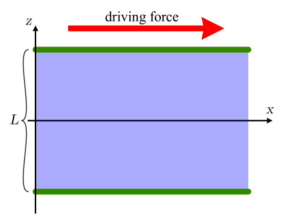
Fig. 1: Cross-section along the $y=0$ plane of the domain for the analytical test case.

In the Newtonian case, the fluid rheology is defined by the dynamic viscosity $\mu=0.1\,\text{Pa}\,\text{s}$. In the Papanastasiou case we have consistency index $\mu_{0}=0.1\,\text{Pa}\,\text{s}$ and yield strength $\tau_{0}=0.0125\,\text{Pa}$, with regularization constant $m=1000\,\text{s}$. In both cases the at-rest density is $\rho_{0}=1\,\text{kg}\,\text{m}^{-3}$.

With the resulting Reynolds number $\text{Re}=6.25\cdot 10^{-1}$, the maximum flow velocity is $u_{\text{max}}=6.25\cdot 10^{-2}\,\text{m}\,\text{s}^{-1}$ (Newton) or $u_{\text{max}}=1.56\cdot 10^{-2}\,\text{m}\,\text{s}^{-1}$ (Papanastasiou), which is in both cases lower than the maximum free-fall velocity across the domain $u_{h}=3.16\cdot 10^{-1}\,\text{m}\,\text{s}^{-1}$. The sound speed is thus taken 20 times higher than $u_{h}$ ($c_{0}=6.32\,\text{m}\,\text{s}^{-1}$).

We validate our results by comparing the velocity profile obtained in GPUSPH against the velocity profile expected by the theory for a stationary flow. The simulations start with a still fluid ($\mathbf{u}=0$); stationary flow is expected to be reached after the viscous relaxation time $t^{\star}=\rho_{0}L^{2}/\mu=10\,\text{s}$. (In the Bingham case a lower relaxation time would be sufficient, due to the higher effective viscosity, but for simplicity we adopt the same $t^{\star}$ used for the Newtonian fluid.)

5.1 Domain discretization

The whole domain is discretized with an initially regular distribution of particles, with constant spacing $\Delta p$, but with slightly different positions depending on the choice of boundary conditions.

When using the dynamic boundary condition, the no-slip condition $\mathbf{u}=\mathbf{u}_{w}=0$ is obtained by placing the first layer of boundary particles at the analytical coordinates of the wall. In contrast, with dummy boundary conditions the analytical position of the wall is halfway between the boundary and fluid particles: the first layer of boundary particles is thus placed $\Delta p/2$ inside the wall (figure 2).

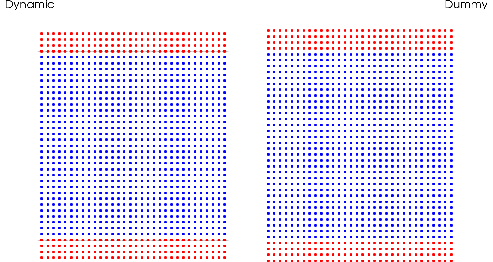
Fig. 2: Cross-section of the domain discretized with the dynamic (left) and dummy (right) boundary models when using the Wendland kernel with smoothing length $1.3\Delta p$. Particles are colored by type (blue for fluid, red for boundary). The number of boundary particle layers is determined by the kernel’s influence radius, and is higher for the other kernel choices discussed in section 5.2.

We test with three different resolutions: $\Delta p=1/16,1/32,1/64$, with the measurement unit being meters. Due to the different discretization, in the dynamic boundary case there is one layer of particles at $z=0$, but not when using dummy boundaries. A central layer of particles can be achieved with dummy boundary conditions by using $1/17,1/33,1/65$ spacings, but this choice leads to somewhat noisier simulations, and the results are not reported here.

5.2 Smoothing kernel choice

The choice of smoothing kernel in SPH has implications in terms of numerical accuracy, stability and performance. According to [31], the commonly used spline of order 3 with radius 2 produces noisy results at low Reynold numbers, and the authors of that paper prefer a computationally more intensive spline of order 5 with radius 3.

The default kernel used in GPUSPH is based on the $\psi_{3,1}$ function defined by Wendland [39], a fifth-order spline of radius 2. We have $W(r,h)=w(r/h)/h^{3}$ with

$$w(q)=\begin{cases}\frac{21}{16\pi}\left(1-\frac{q}{2}\right)^{4}(2q+1)&q\leq 2\\ 0&q>2\end{cases},$$

and $F(r,h)=f(r/h)/h^{5}$ with

$$f(q)=\begin{cases}\frac{105}{128\pi}(q-2)^{3}&q\leq 2\\ 0&q>2\end{cases}.$$

With a smoothing factor of $1.3$, and thus an influence radius of $2.6\Delta p$, each particle will have around 80 neighbors.

Another option is the normalized truncated Gaussian of radius $k=3$. We have then

$$w(q)=\begin{cases}(\exp(-q^{2})-\exp(-k^{2}))/w_{G}&q\leq k\\ 0&q>k\end{cases}$$

where $w_{G}=\pi^{3/2}\operatorname{erf}(k)-2\pi/3\exp(-k^{2})k(3+2k^{2})$ is the normalization factor, and

$$f(q)=\begin{cases}2\exp(-q^{2})/w_{G}&q\leq k\\ 0&q>k\end{cases}.$$

With the same smoothing factor used for the Wendland kernel, and thus an influence radius of $3.9\Delta p$, each particle will have around 250 neighbors.

Due to the larger influence radius and the use of transcendental functions, the Gaussian kernel is around 4 times more computationally expensive than the Wendland kernel. The larger influence radius also requires about 2 times more memory to store the neighbors list of each particle (in the default configuration, GPUSPH will reserve memory for up to 128 neighbors per particle). However, as we shall see, the Gaussian kernel can give more accurate results, and there are additional benefits to a larger influence radius in the semi-implicit formulation.

5.3 Newtonian results

The expected velocity profile for a Newtonian fluid in the plane Poiseuille flow is a parabola with maximum velocity in the middle, and null velocity at the planes (due to the no-slip boundary condition):

$$u(z)=\frac{1}{2}\frac{\rho_{0}g}{\mu}\left(\frac{L^{2}}{4}-z^{2}\right).$$

Convergence

In its simplicity, this test case presents some peculiarities, that are illustrated in figures 3 and 4. We observe that using the Wendland kernel (figure 3) with a smoothing factor for $1.3$ produces results that are largely independent from the resolution; additionally, the velocity profile, while qualitatively correct, is consistently overestimated. The Gaussian kernel, on the other hand, (figure 4), shows convergence towards the correct solution.

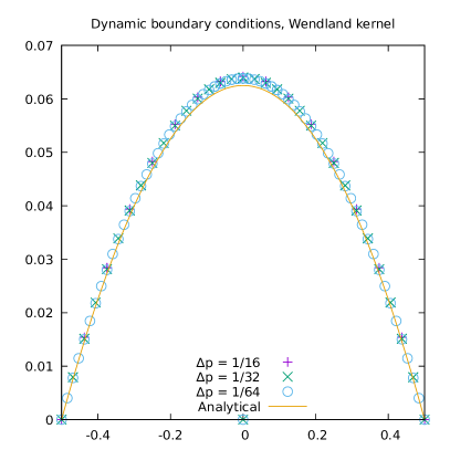
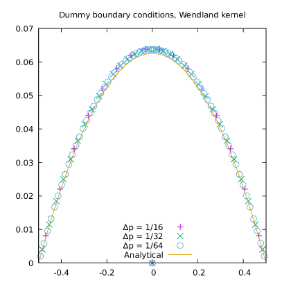
Fig. 3: Analytical and numerical velocity profiles of the plane Poiseuille flow for a Newtonian fluid, with dynamic (left) and dummy boundary (right) conditions, using the Wendland smoothing kernel.

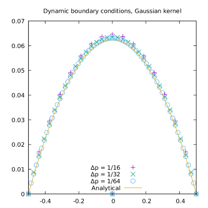
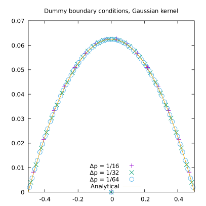
Fig. 4: Analytical and numerical velocity profiles of the plane Poiseuille flow for a Newtonian fluid, with dynamic (left) and dummy (right) boundary conditions, using the Gaussian smoothing kernel.

In both cases, we remark the lack of noise in the results: we are plotting the results for all of the fluid particles (and, with dynamic boundaries, the first layer of boundary particles), and there is no spread in any direction, indicating that all particles with the same $z$ coordinate have numerically the same velocity, regardless of their $x$ or $y$ position.

The actual numerical performance with the two smoothing kernels is shown in table 1. We can remark that the dummy boundary conditions consistently provide lower error and higher convergence rates compared to the dynamic boundary conditions, as expected. The Gaussian kernel also provides better results in all respects, and in particular it shows convergence towards the analytical solution, whereas the Wendland kernel seems to converge towards a solution which is $2\%$ higher than the analytical solution.

Kernel $\dfrac{1}{\Delta p}$ Dynamic Dummy $l_{1}$ rate $l_{1}$ $l_{2}$ rate $l_{2}$ $l_{1}$ rate $l_{1}$ $l_{2}$ rate $l_{2}$ Gaussian $16$ $2.083\cdot 10^{-3}$ n.a. $2.153\cdot 10^{-3}$ n.a. $3.615\cdot 10^{-4}$ n.a. $3.713\cdot 10^{-4}$ n.a. $32$ $1.033\cdot 10^{-3}$ $1.01$ $1.050\cdot 10^{-3}$ $1.04$ $4.081\cdot 10^{-5}$ $3.15$ $5.087\cdot 10^{-5}$ $2.87$ $64$ $5.097\cdot 10^{-4}$ $1.02$ $5.139\cdot 10^{-4}$ $1.03$ $2.010\cdot 10^{-5}$ $1.02$ $2.096\cdot 10^{-5}$ $1.28$ Wendland $16$ $1.210\cdot 10^{-3}$ n.a. $1.325\cdot 10^{-3}$ n.a. $1.227\cdot 10^{-3}$ n.a. $1.282\cdot 10^{-3}$ n.a. $32$ $1.061\cdot 10^{-3}$ $0.19$ $1.133\cdot 10^{-3}$ $0.23$ $9.598\cdot 10^{-4}$ $0.35$ $1.032\cdot 10^{-3}$ $0.31$ $64$ $9.490\cdot 10^{-4}$ $0.16$ $1.024\cdot 10^{-3}$ $0.15$ $8.792\cdot 10^{-4}$ $0.13$ $9.585\cdot 10^{-4}$ $0.11$ Wendland $16$ $4.288\cdot 10^{-4}$ n.a. $4.576\cdot 10^{-4}$ n.a. $3.916\cdot 10^{-4}$ n.a. $3.929\cdot 10^{-4}$ n.a. ($102\%\mathbf{u}$) $32$ $2.283\cdot 10^{-4}$ $0.91$ $2.338\cdot 10^{-4}$ $0.97$ $1.260\cdot 10^{-4}$ $1.64$ $1.294\cdot 10^{-4}$ $1.60$ $64$ $1.158\cdot 10^{-4}$ $0.98$ $1.204\cdot 10^{-3}$ $0.96$ $4.573\cdot 10^{-5}$ $1.46$ $5.435\cdot 10^{-5}$ $1.25$

Table 1: $l_{1}$ and $l_{2}$ norms and convergence rate of the plane Poiseuille flow for a Newtonian fluid. Results are for the implicit formulation, with dynamic and dummy boundary conditions, with both the Gaussian and Wendland kernel. The Wendland kernel is also compared against the solution it appears to converge to.

In practical applications, a $2\%$ may be considered acceptable, and as we shall see in the next section, the actual performance of the Wendland kernel is also problem-dependent. Still, one might be led to ask about the reason for this discrepancy.

The difference between the Gaussian and Wendland kernel is reminiscent of the difference between splines of order 3 and 5 reported by Morris [31] (with the latter providing better results), but our results shed additional light on the root cause: since our Wendland kernel is an order 5 spline (like the best one used by Morris), but with radius 2, it would seem that the discrepancy is not to be sought (only) in the behavior of the second derivative of the kernel, but also in the size of the kernel support itself.

In fact, a recent result by Violeau & Fonty [40] shows that the smoothing error is actually proportional to the square of the kernel’s standard deviation $\sigma$, rather than the smoothing length $h$. Since the $\sigma/h$ ratio is kernel-dependent, the choice of smoothing factor should be kernel-dependent to attain similar results, whereas in our case we are using a fixed one for both kernel choices.

Considering that $(\sigma/h)^{2}=4/15$ for the Wendland kernel [40], and $(\sigma/h)^{2}\approx 1/2$ for the (truncated) Gaussian kernel, we can expect that using a smoothing factor about $15/8$ times larger than the one used for the Gaussian kernel would lead to comparable convergence ratios when using the Wendland kernel. This is confirmed by running the Wendland case with a smoothing factor of $2.5$ rather than the usual $1.3$ (table 2).

Dynamic Dummy $1/\Delta p$ $l_{1}$ rate $l_{1}$ $l_{2}$ rate $l_{2}$ $l_{1}$ rate $l_{1}$ $l_{2}$ rate $l_{2}$ $16$ $5.436\cdot 10^{-3}$ n.a. $5.625\cdot 10^{-3}$ n.a. $6.648\cdot 10^{-4}$ n.a. $7.797\cdot 10^{-4}$ n.a. $32$ $2.588\cdot 10^{-3}$ $1.07$ $2.673\cdot 10^{-3}$ $1.07$ $5.095\cdot 10^{-5}$ $3.71$ $1.502\cdot 10^{-4}$ $2.38$ $64$ $1.300\cdot 10^{-3}$ $0.99$ $1.322\cdot 10^{-3}$ $1.02$ $5.941\cdot 10^{-5}$ $-0.22$ $6.696\cdot 10^{-5}$ $1.17$

Table 2: $l_{1}$ and $l_{2}$ norms and ratios for growing resolutions of the plane Poiseuille flow for a Newtonian fluid with dynamic and dummy boundary conditions, using the Wendland kernel with smoothing factor $2.5$.

Indeed, in this case the Wendland kernel exhibits convergence properties similar to those seen for the Gaussian kernel with smoothing factor $1.3$, at least up to numerical limits (seen in table 2 for the dummy boundary case in $l_{1}$ norm at $\Delta p=1/64$). We remark also that the average number of neighbors for Wendland/$2.5$ is also about twice as large as the number of neighbors in the Gaussian/$1.3$ case, which is what we expect given the different values of $\sigma/h$ for the two kernels.

Computational performance

Due to the simplicity of the geometry in this test case, the results are essentially the same for both the implicit and explicit formulation. Moreover, the implicit formulation is actually slower than the explicit formulation, since the viscosity of the fluid is not high enough, and the dominant time-step limitation comes from the sound speed at most resolutions (table 3).

Runtime Kernel $\dfrac{1}{\Delta p}$ Dynamic Dummy $\Delta t_{c}$ $\Delta t_{\nu}$ Explicit Implicit Explicit Implicit Gaussian $16$ $3.85\cdot 10^{-3}$ $8.25\cdot 10^{-3}$ $7.7\cdot 10^{0}$ $4.6\cdot 10^{1}$ $7.8\cdot 10^{0}$ $6.8\cdot 10^{1}$ $32$ $1.93\cdot 10^{-3}$ $2.06\cdot 10^{-3}$ $4.5\cdot 10^{1}$ $4.3\cdot 10^{2}$ $4.9\cdot 10^{1}$ $7.4\cdot 10^{2}$ $64$ $9.63\cdot 10^{-4}$ $5.16\cdot 10^{-4}$ $1.3\cdot 10^{3}$ $9.7\cdot 10^{3}$ $1.4\cdot 10^{3}$ $1.3\cdot 10^{4}$ Wendland $16$ $3.85\cdot 10^{-3}$ $8.25\cdot 10^{-3}$ $3.3\cdot 10^{0}$ $2.4\cdot 10^{1}$ $3.6\cdot 10^{0}$ $3.3\cdot 10^{1}$ $32$ $1.93\cdot 10^{-3}$ $2.06\cdot 10^{-3}$ $2.0\cdot 10^{1}$ $2.5\cdot 10^{2}$ $2.1\cdot 10^{1}$ $3.7\cdot 10^{2}$ $64$ $9.63\cdot 10^{-4}$ $5.16\cdot 10^{-4}$ $4.8\cdot 10^{2}$ $4.3\cdot 10^{3}$ $5.0\cdot 10^{2}$ $5.6\cdot 10^{3}$

Table 3: Time-step limitation from speed of sound ($\Delta t_{c}$) and viscosity ($\Delta t_{\nu}$), and effective simulation runtimes in seconds for both boundary models with the explicit and semi-implicit formulations in the Newtonian case. The kernel choice affects the runtime, but not the time-step.

Even at the highest resolution, where the viscous time-step limitation becomes dominant, the benefit of being limited only by the sound speed in the implicit case is not sufficient to offset the higher computational cost of the semi-implicit formulation. However, it is interesting to remark that, while the runtimes with the Gaussian kernel are consistently more than twice longer than with the Wendland kernel in the explicit case, for the semi-implicit formulation the ratio is lower.

Both of these phenomena are explained by the difference between the number of iterations required to solve the implicit system, and the time-step choice.

Indeed, a full semi-implicit step at the highest resolution, requires on average 3 (dynamic boundary) to 5 (dummy boundary) BiCGSTAB iterations with the Wendland kernel, but only 1 (dynamic boundary) to 3 (dummy boundary) iterations with the Gaussian kernels. Because of this, the performance loss of the Gaussian kernel computation is partially compensated by the faster convergence of the solver.

However, a full semi-implicit step is between $10\times$ (dynamic, Gaussian) and $15.1\times$ (dummy, Gaussian) longer than the time needed for a full explicit step. By contrast, adopting the semi-implicit formulation leads to a reduction in the number of time-steps (thanks to the removal of the viscous time-step constraint) which is much more modest ($1.88\times$).

The performance difference between the explicit and semi-implicit scheme is in line with the observations made in [21], and suggests that the turning point for the advantage of the semi-implicit formulation would be a time-step constraint ratio of $20\times$ or more. This could be achieved with an even higher resolution, but is better illustrated by the non-Newtonian test-case presented in the next section.

We remark that the implicit solver itself converges pretty quickly, but this is only when implemented as described in section 4.2. The standard BiCGSTAB implementation, in single precision, is affected by frequent stalls, leading to much noisier results, or even failing to converge altogether even at the moderate resolution.

Note that for the dynamic boundary case we can also use the CG to solve the linear system: tested with the Wendland kernel, runtimes are around $10\%$ faster than the BiCGSTAB solver, despite the larger number of iterations needed for convergence (4 instead of 1 at the lowest resolution, 7 instead of 3 at the highest). The performance benefit of the CG is thus not sufficient to make the semi-implicit formulation convenient over the explicit scheme at these resolutions.

5.4 Papanastasiou case

For the Papanastasiou rheology, we compare the numerical results against the analytical solution for the velocity profile of a non-regularized Bingham fluid. The flow is divided into a yielded $\lVert\tau\rVert_{II}\geq\tau_{0}$ and unyielded $\lVert\tau\rVert_{II}<\tau_{0}$ regions (figure 5). The unyielded region (plug) spans the area $z_{-}<z<z_{+}$, with $z_{+}=\tau_{0}/(\rho_{0}g)$ and $z_{-}=-z_{+}$.

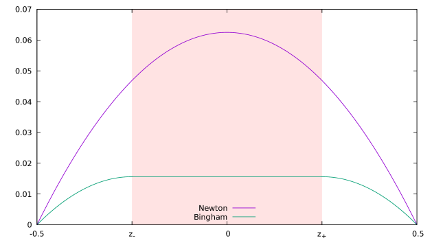
Fig. 5: Velocity profile for the plane Poiseuille flow of a Bingham fluid, highlighting the presence of a plug (unyielded region) and its shallowing effect in comparison to a Newtonian fluid.

In the yielded region, the velocity profile is parabolic, with:

$$u(z)=\frac{1}{2}\frac{\rho_{0}g}{\mu_{0}}\left(\frac{L^{2}}{4}-z^{2}\right)-\frac{\tau_{0}}{\mu_{0}}\left(\frac{L}{2}-\left|z\right|\right),$$

whereas the plug moves at the plug velocity

$$u_{p}=u(z_{-})=u(z_{+})=\left(\frac{L}{2}-\frac{\tau_{0}}{\rho_{0}g}\right)\frac{\rho_{0}gL/2-\tau_{0}}{2\mu_{0}}.$$

Convergence

In this test-case, the Wendland kernel with the standard smoothing factor of $1.3$ shows good convergence to the analytical velocity profile (figure 6), even better than the Gaussian kernel (figure 7).

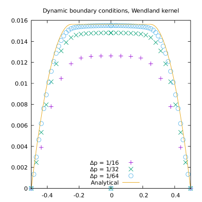
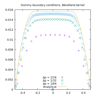
Fig. 6: Analytical and numerical velocity profiles of the plane Poiseuille flow for a Papanastasiou fluid, with dynamic (left) and dummy (right) boundary conditions, using the Wendland smoothing kernel.

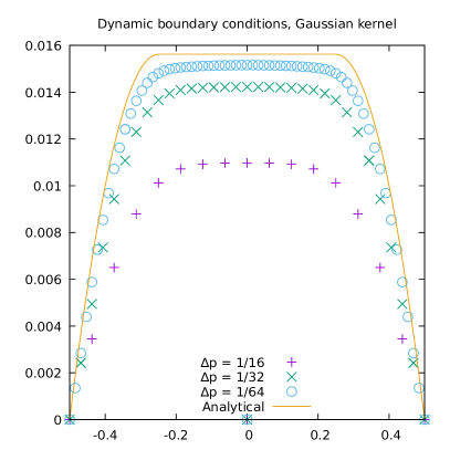
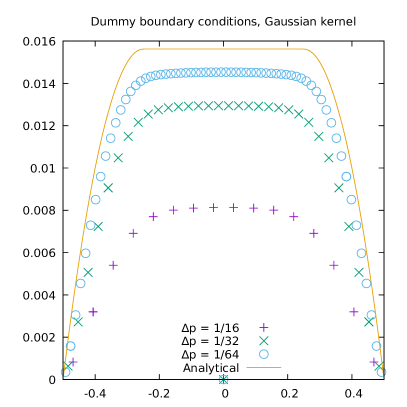
Fig. 7: Analytical and numerical velocity profiles of the plane Poiseuille flow for a Papanastasiou fluid, with dynamic (left) and dummy (right) boundary conditions, using the Gaussian smoothing kernel.

Again, as in the Newtonian case, the results are very clean (no discernible discrepancy in the velocity for particles at the same $z$ coordinate). In contrast to the Newtonian case, however, the dummy boundary model performs slightly worse than the dynamic boundaries. While this can be at least partially ascribed to the lower effective particle spacing used in the setup with the dummy boundary compared to the dynamic boundary case, the results suggest that further research is necessary to improve the behavior of the dummy boundary formulation in the case of shear-dependent effective viscosity.

Details about the discrete error norms and convergence rates are shown in table 4. An important point to remark is that these results include both the discretization error from the numerical method and the discrepancy between the analytical solution for a Bingham rheology versus the solution for its Papanastasiou regularization. Despite the influence of the latter, however, the results obtained are still very good.

Kernel $\dfrac{1}{\Delta p}$ Dynamic Dummy $l_{1}$ rate $l_{1}$ $l_{2}$ rate $l_{2}$ $l_{1}$ rate $l_{1}$ $l_{2}$ rate $l_{2}$ Gaussian $16$ $4.569\cdot 10^{-3}$ n.a. $4.769\cdot 10^{-3}$ n.a. $7.027\cdot 10^{-3}$ n.a. $7.227\cdot 10^{-3}$ n.a. $32$ $1.720\cdot 10^{-3}$ $1.41$ $1.790\cdot 10^{-3}$ $1.41$ $2.928\cdot 10^{-3}$ $1.26$ $2.982\cdot 10^{-3}$ $1.27$ $64$ $7.245\cdot 10^{-4}$ $1.25$ $7.635\cdot 10^{-4}$ $1.23$ $1.336\cdot 10^{-3}$ $1.13$ $1.360\cdot 10^{-3}$ $1.13$ Wendland $16$ $3.009\cdot 10^{-3}$ n.a. $3.232\cdot 10^{-3}$ n.a. $4.724\cdot 10^{-3}$ n.a. $4.815\cdot 10^{-3}$ n.a. $32$ $1.138\cdot 10^{-3}$ $1.58$ $1.196\cdot 10^{-3}$ $1.43$ $1.861\cdot 10^{-3}$ $1.34$ $1.894\cdot 10^{-3}$ $1.34$ $64$ $3.715\cdot 10^{-4}$ $1.61$ $6.833\cdot 10^{-4}$ $1.47$ $7.339\cdot 10^{-4}$ $1.34$ $7.631\cdot 10^{-4}$ $1.31$

Table 4: $l_{1}$ and $l_{2}$ norms and ratios for growing resolutions of the plane Poiseuille flow for a Papanastasiou fluid with dynamic and dummy boundary conditions.

Computational performance

When simulating a non-Newtonian fluid, or more in general a fluid with non-constant viscosity, the upper bound on the time-step controlled by the viscosity should change according to the highest effective viscosity encountered during the simulation. However, in this case the presence of the plug (where the viscosity is always the maximum possible value) effectively enforces the same time-step throughout the whole simulation. Moreover, due to the (finite but) very high viscosity of the plug, the viscous condition on the time-step is always dominant when using the explicit integration scheme (table 5).

Runtime Kernel $\dfrac{1}{\Delta p}$ Dynamic Dummy $\Delta t_{c}$ $\Delta t_{\nu}$ Explicit Implicit Explicit Implicit Gaussian $16$ $3.85\cdot 10^{-3}$ $6.55\cdot 10^{-5}$ $7.1\cdot 10^{2}$ $1.3\cdot 10^{2}$ $7.3\cdot 10^{2}$ $1.8\cdot 10^{2}$ $32$ $1.93\cdot 10^{-3}$ $1.64\cdot 10^{-5}$ $1.0\cdot 10^{4}$ $1.7\cdot 10^{3}$ $1.2\cdot 10^{4}$ $2.6\cdot 10^{3}$ $64$ $9.63\cdot 10^{-4}$ $4.09\cdot 10^{-6}$ $3.6\cdot 10^{5}$ $4.3\cdot 10^{4}$ $3.9\cdot 10^{5}$ $6.1\cdot 10^{4}$ Wendland $16$ $3.85\cdot 10^{-3}$ $6.55\cdot 10^{-5}$ $2.7\cdot 10^{2}$ $7.4\cdot 10^{1}$ $3.1\cdot 10^{2}$ $9.5\cdot 10^{1}$ $32$ $1.93\cdot 10^{-3}$ $1.64\cdot 10^{-5}$ $4.3\cdot 10^{3}$ $1.0\cdot 10^{3}$ $4.9\cdot 10^{3}$ $1.4\cdot 10^{3}$ $64$ $9.63\cdot 10^{-4}$ $4.09\cdot 10^{-6}$ $1.2\cdot 10^{5}$ $2.0\cdot 10^{4}$ $1.3\cdot 10^{5}$ $2.7\cdot 10^{4}$

Table 5: Time-step limitation from speed of sound ($\Delta t_{c}$) and viscosity ($\Delta t_{\nu}$), and effective simulation runtimes in seconds for both boundary models with the explicit and semi-implicit formulations in the Papanastasiou case.

The number of BiCGSTAB iterations needed to converge is also higher in this case; as remarked also in [21], this is most likely due to the diagonal dominance of the matrix (for the rows that are SDD) diminishing as the viscosity grows higher. With the Wendland kernel, the implicit solver converges in 12 iterations on average at the lowest resolution with the dynamic boundary model, (14 for the dummy boundary model), in 18 iterations on average at the moderate resolution (21 for the dummy boundary model), and in 25 iterations at the highest resolution (32 for the dummy boundary model).

At the highest resolution, with both boundary formulations, the BiCGSTAB solver is sometimes affected by early returns due to stalls. However, the only component that is affected is the transverse direction $y$, where the velocity component should be zero analytically. Numerically, the order of the $y$ component of the velocities is $10^{-8}$, which is negligible, but still manages to affect the solver. This is the only case where even our restructured BiCGSTAB (section 4.2) is affected by the low numerical precision.

Overall, the semi-implicit formulation in this case is 3 to 5 times faster than the explicit scheme, when using the Wendland kernel. As in the Newtonian test case, the break-even point can be computed comparing the ratio between the viscous and sound-speed time-step limitation with the runtime for a single time-step, which in the semi-implicit case is proportional to the number of iterations needed by the implicit solver.

While in the Newtonian case the break-even was computed to be around $20\times$ with an average of 5 implicit solver iterations, with the slower convergence in the Papanastasiou case the break-even is expected to be 2 to 6 times higher (thus $40\times$ to $120\times$) depending on resolution, while we have $\Delta t_{c}/\Delta t_{\nu}$ ranging from $170$ (low resolution) to $425$ (high resolution). The ratio of ratios matches up with the effective speed-up achieved.

We can also observe again that the computationally more expensive Gaussian kernel benefits more from the semi-implicit scheme, thanks to the faster convergence (6/11/16 iterations on average at the low/middle/high resolution with the dynamic boundary conditions, and 9/14/21 with the dummy boundary conditions.) This leads to simulations that are over 8 times faster with the semi-implicit scheme than the explicit formulation, at the highest resolution tested.

5.5 Cross-flow velocities

Even though the Poiseuille flow is essentially uni-directional, we see particles developing a non-zero velocity in the cross-flow directions $y$ (periodic) and $z$ (wall-to-wall) directions, reaching at most in the order of $10^{-8}\,\text{m}\,\text{s}^{-1}$ and $10^{-5}\,\text{m}\,\text{s}^{-1}$ respectively by the end of the runs. These are independent of the integration scheme, and are related instead to the nature of the adopted formulation for the viscous term, that does not strictly conserve angular momentum [41].

As shown in the results, the development of these spurious velocities does not affect the numerical results in the considered timeframe (although they should be addressed for longer simulations). However, they do influence the convergence speed of the linear solver when adopting the semi-implicit scheme, due to the resulting vanishing but non-zero tolerance value in the linear system for the corresponding coordinates.

The effect is particularly strong in the periodic direction $y$, where the velocities (and the corresponding thresholds for convergence) are significantly smaller, often bordering the minimum representable single-precision floating-point value FLT_MIN.

Consider as an example the Papanastasiou case with dummy boundary conditions and $\Delta p=1/64$: during the corrector step at iteration 390 the thresholds for $x$, $y$ and $z$ are respectively $2.31\cdot 10^{-16}$, $9.37\cdot 10^{-38}$ and $2.48\cdot 10^{-24}$. After 42 solver steps, the algorithm bails out due to a stall in the convergence of the $y$ component of the velocity, with residual norms $2.89\cdot 10^{-22}$, $3.70\cdot 10^{-37}$ (failed to converge) and $2.15\cdot 10^{-27}$ respectively. The user is notified of the failure, and the simulation continues. In this case, this is an acceptable loss of accuracy, and we decide to keep the results.

While these extreme situations are an excellent test-bed for the robustness of our improved CG and BiCGSTAB solvers, in practical applications they may lead to undesired increases in runtimes due to the slower convergence. Heuristics (either automatic or user-guided) to determine negligible components for the stopping criterion are currently being explored as a possible solution.

6 Test case: flow in a periodic lattice of cylinders

Since the plane Poiseuille flow is effectively a simple unidirectional shearing flow, it doesn’t fully capture the effect of particle disorder on the solver robustness within the timeframe needed to reach a steady-state flow: perturbations are small and the effect is mostly seen in the loss of convergence speed in the cross-flow directions as pointed out at the end of the previous section.

To illustrate the semi-implicit solver performance in a more complex test case, including the effect of a distorted (non-uniform) particle distributions, we show here the results in the case of a flow in a periodic lattice of cylinders. Following [31], two variants of the test case are presented, one with $Re=1$ (which we refer to as Low Reynolds Number or LRN case), and one with $Re=0.03$ (Very Low Reynolds Number or VLRN case).

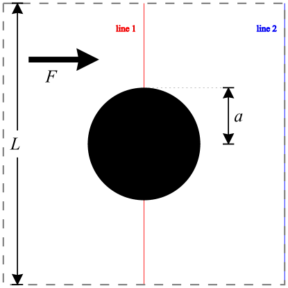
Fig. 8: Geometry for the flow in a periodic lattice of cylinders test cases. The marked lines 1 and 2 are the ones through which the velocity profiles are taken to validate our results.

LRN VLRN $F$ ($\text{ms}^{-2}$) $1.5\cdot 10^{-7}$ $5\cdot 10^{-5}$ $\nu$ ($\text{m}^{2}\text{s}^{-1}$) $10^{-6}$ $10^{-4}$ $c_{0}$ ($\text{ms}^{-1}$) $6\cdot 10^{-4}$ $10^{-2}$ $t_{\text{max}}$ (s) $1.6\cdot 10^{3}$ / $8\cdot 10^{3}$ $7\cdot 10^{2}$ / $1.4\cdot 10^{5}$

Table 6: Parameters for the Low Reynolds Number (LRN) and Very Low Reynolds Number (VLRN) flows in a periodic lattice of cylinders. The two end times $t_{\text{max}}$ refer to the “short” and “long” simulations as discussed in the text.

In both cases the domain is a 2D periodic square cell with side $L=0.1\,\text{m}$, with a cylinder of radius $a=0.02\,\text{m}$ centered in it (Figure 8). The fluid is initially at-rest, subject to a driving force in the $x$ direction. The magnitude $F$ of the driving force per unit mass, kinematic viscosity $\nu$ and at-rest sound-speed $c_{0}$ depend on the test case and are illustrated in Table 6. We use $\rho_{0}=1\,\text{kg}\,\text{m}^{-3}$ in both test cases.

Especially in the VLRN, the effect of particle disorder cannot be fully appreciated when the steady state is reached, so we run both LRN and VLRN for a “short” time (to the steady state) as well as for a “long” time. The simulated runtimes are also indicated in Table 6, and correspond approximately to the number of timesteps indicated by [31].

6.1 Domain discretization

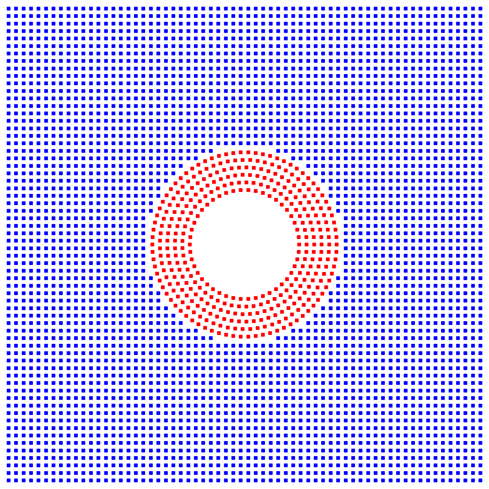
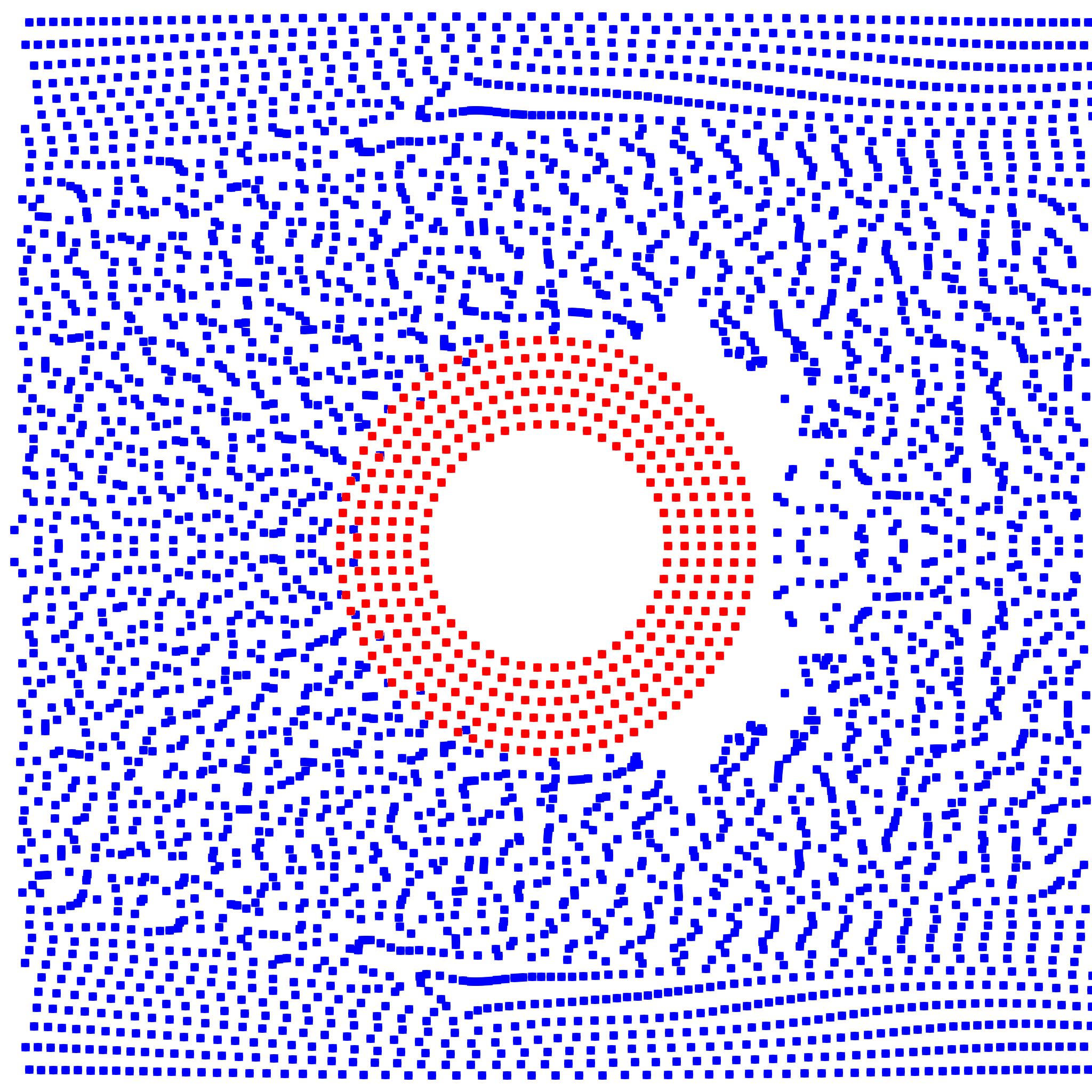
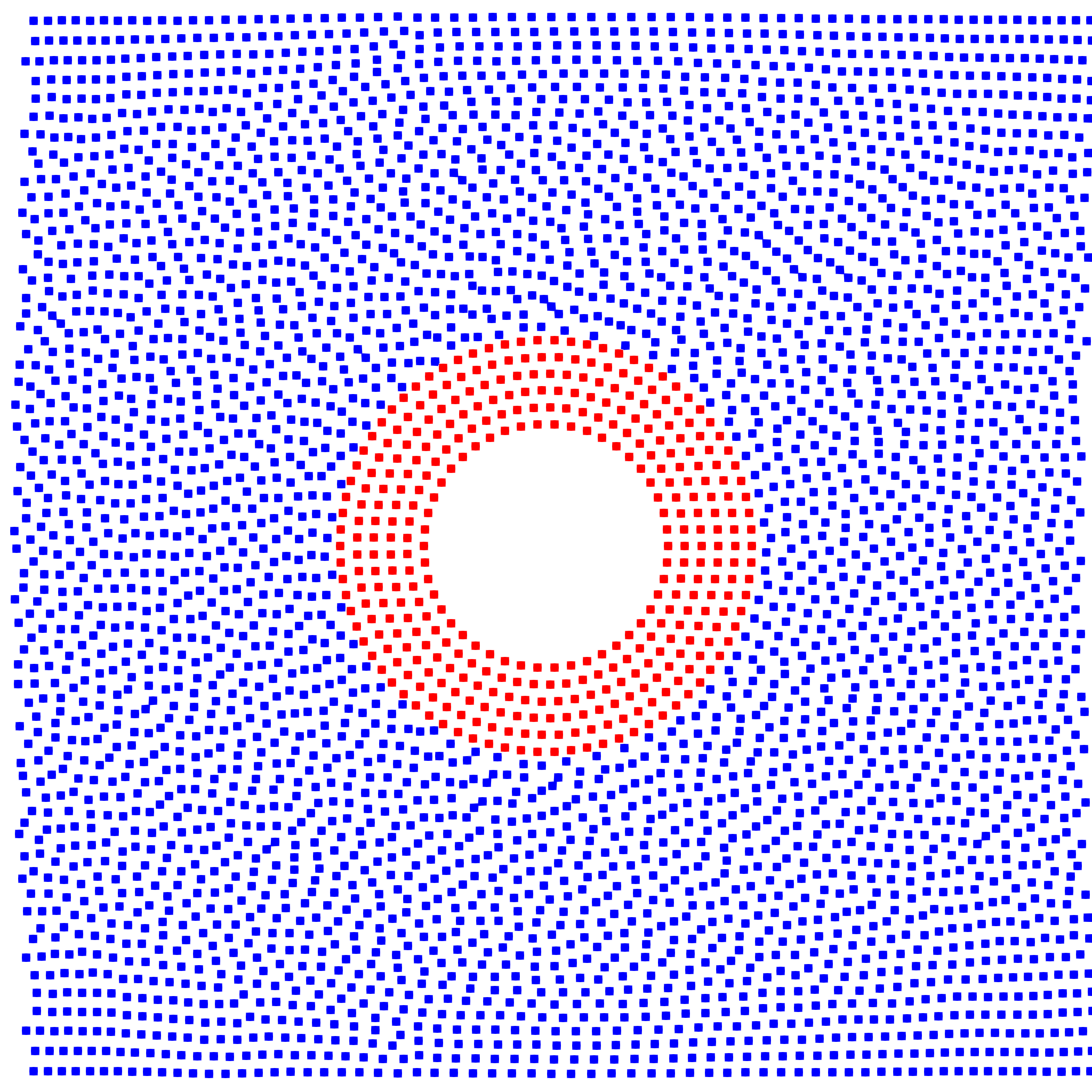
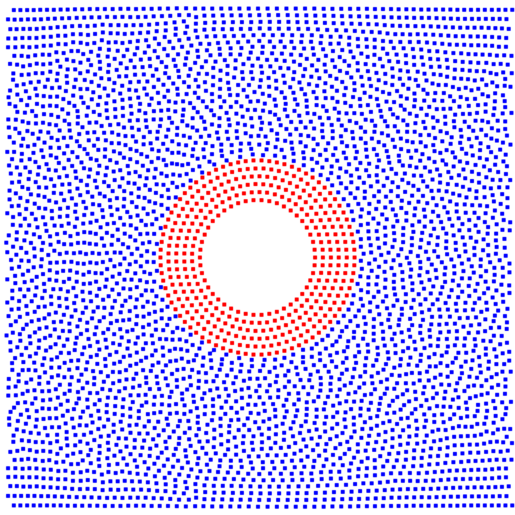
Fig. 9: Initial particle configuration (top left), effect of tensile instability with Cole’s equation of state (top right), and layout at $t=4000\,\text{s}$ with the explicit (bottom left) and semi-implicit (bottom right) integrators when using the simplified equation of state.

Our initial setup (shown in the top left of Figure 9) has a regularly spaced grid of particles for the fluid stopping at a distance of $\Delta p/2$ from the cylinder surface, whereas the cylinder itself is discretized with dummy boundary particles distributed along concentric circles starting $\Delta p/2$ inside.

For a complete assessment of the computational performance, we run simulations with a number of resolutions, defined in terms of the number of particles spanning the length $L$ (p.p.$L$, particles per $L$), starting from 64 p.p.$L$ (close to the resolution used in [31]) and doubling up to 2048 p.p. $L$. The ”long” simulations in the VLRN case were only run up to a 512 p.p.$L$ resolution due to the prohibitive computational times for the explicit integration scheme. Some of the considerations about the choices of SPH formulation will show examples from the lowest resolution, and the ”long” run validation tests will show the results at the highest resolution.

The well-known tensile instability of SPH [42] leads to numerical problems such as particle clumping and the creation of voids in the low-pressure region past the cylinder when using Cole’s equation of state (1), as show in Figure 9 (top right). Since the test case does not feature a free surface, the issue can be solved by adopting the simpler equation of state

$$P(\rho)=c_{0}^{2}\rho$$

proposed by [31]. We remark that the choice of integrator has no influence on the tensile instability, although it does result in different particle distributions in the long term (as shown in the bottom to subfigures of Figure 9).

To reduce the numerical noise in the pressure field, we adopt the density diffusion mechanism described in [43], adding a diffusive term to the mass continuity equation (4)

$$\frac{D\rho_{\beta}}{Dt}=\sum_{\alpha}m_{\alpha}\mathbf{u}_{\alpha\beta}\cdot\mathbf{r}_{\alpha\beta}F_{\alpha\beta}+\xi hc_{0}\sum_{\alpha}m_{\alpha}\Psi_{\alpha\beta}F_{\alpha\beta}$$

where $\xi\in[0,1]$ is the diffusive coefficient, for which we use $\xi=0.1$, and

$$\Psi_{\alpha\beta}=\begin{cases}2\left(\dfrac{P_{\beta}}{P_{\alpha}}-1\right)&\text{if }\dfrac{\left|P_{\alpha\beta}\right|}{\rho_{\beta}\left|\mathbf{g}\cdot\mathbf{r}_{\alpha\beta}\right|}>1\\ 0&\text{otherwise}\end{cases}$$

is the diffusive contribution. We prefer this to the more recent and more sophisticated forms proposed for the diffusive term [44, 45], because these come at the cost of higher computational loads and are aimed at improving the solution near the free surface, which is not present in our test cases.

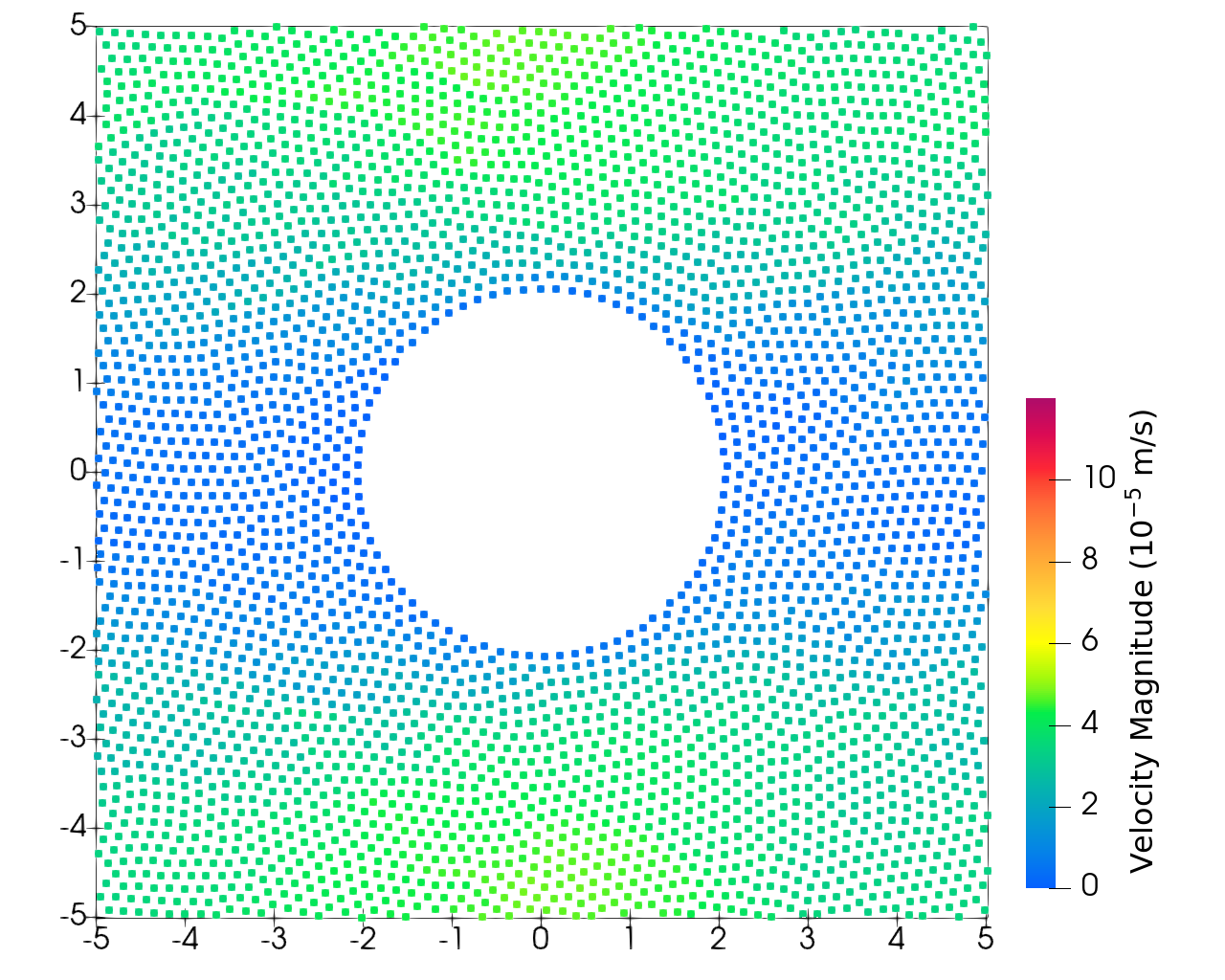
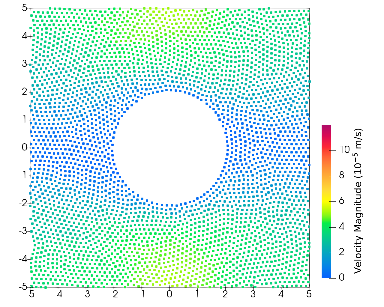
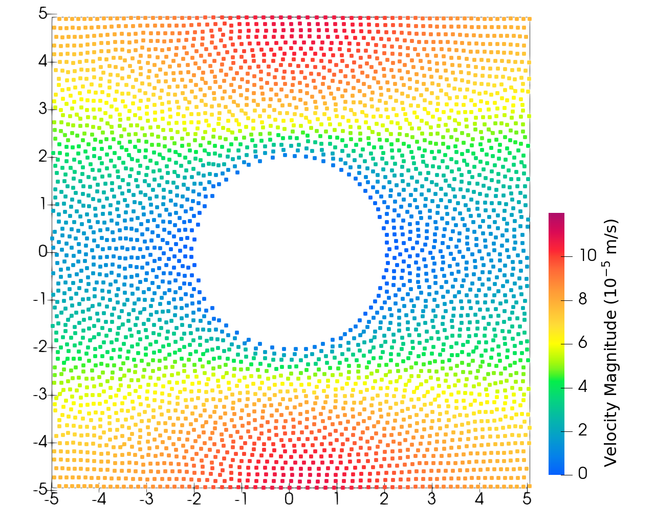
Fig. 10: Distribution of the velocity magnitude at a steady state for the explicit (left) and semi-implicit (right) integrator when using smoothing factor $1.3$ (top) versus $2.25$ (bottom) in the LRN case at the lowest resolution employed in our tests.

We use the Wendland kernel described in section 5.2, with a smoothing factor for $2.25$. The choice of the smoothing factor is dictated by the excessive numerical dissipation observed at smaller values (Figure 10). Indeed, in this test case the default value of $1.3$ for the smoothing radius results in an effective speed that is about 50% of the expected value at a steady state. Such excessive viscous dissipation is independent from the chosen integration scheme, and has been thoroughly studied in the context of SPH application to gravity waves (see e.g. [46, 47, 48, 49]), with the most common solution being the adoption of larger smoothing factors [46], sometimes coupled with appropriate kernel choices [50, 47].

The larger smoothing factor is, in our case, a simple and effective solution, consistent with the already-discussed results seen for the plane Poiseuille test case (section 5.3). Additionally, our test-case does not have a free surface, and is thus immune to the “rarifying” free surface side-effect of larger smoothing factors when studying gravity waves discussed e.g. in [51]. Alternative strategies such as the use of kernel corrections [52, 53, 51], that may require specific adaptation to the semi-implicit numerical scheme are being considered as future work.

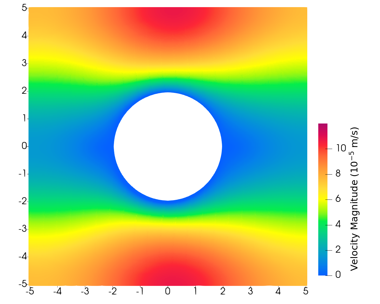
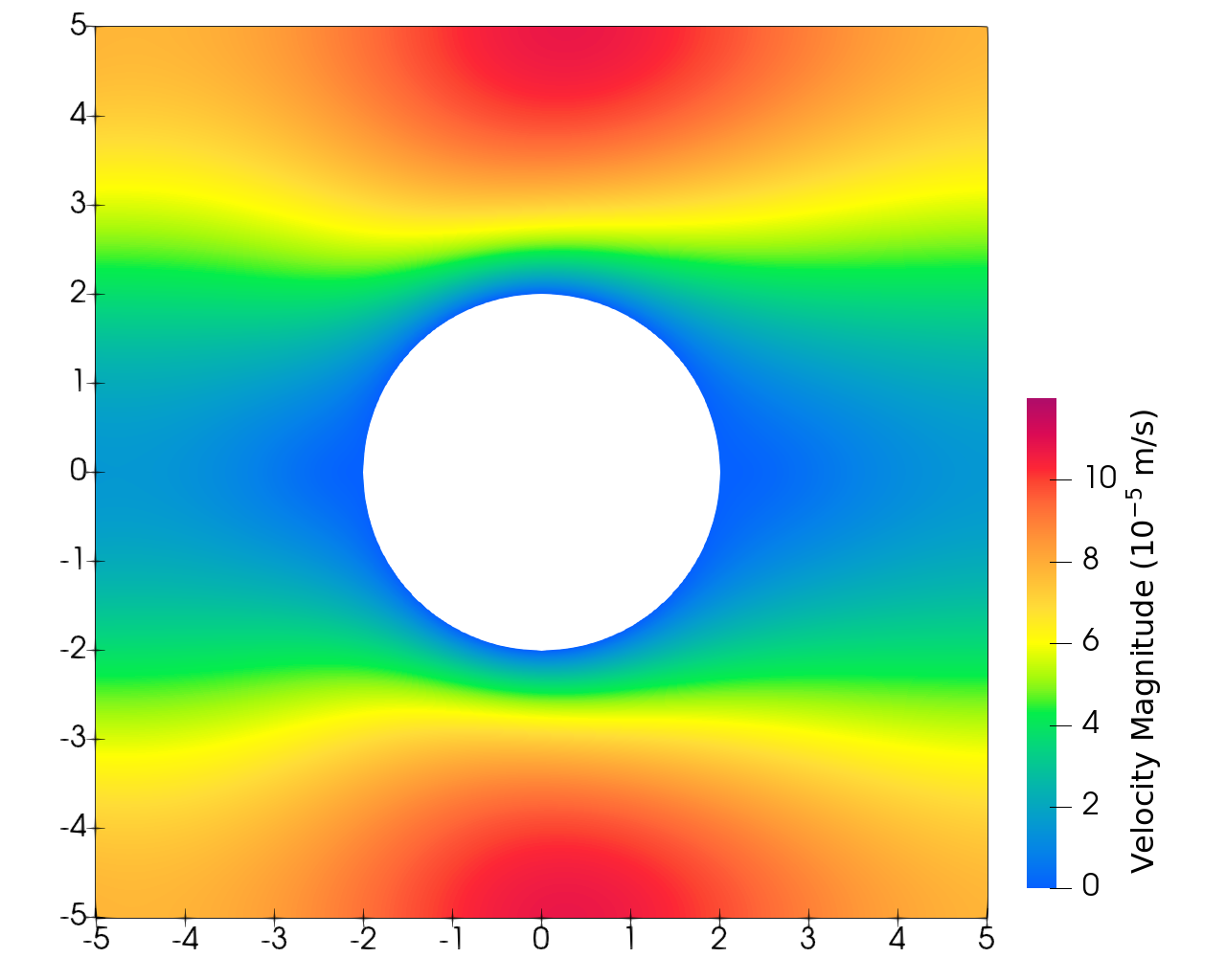
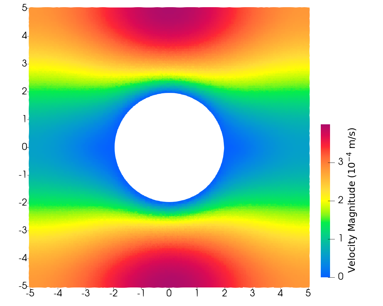
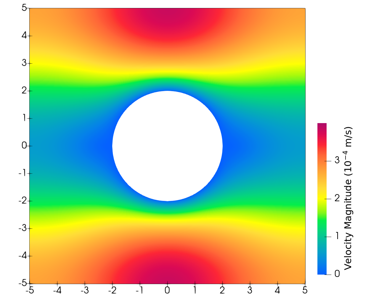
Fig. 11: Distribution of the velocity magnitude for the LRN (top) and VLRN (bottom) cases in the ”long” run for our semi-implicit integrator at high p.p.$L$ (left), explicit integrator at high p.p.$L$ (middle) versus the FVE model used for validation (right). The high p.p.$L$ is 2048 for the LRN case and 512 for the VLRN case. Axes are in units of $10^{-2}\,\text{m}$.

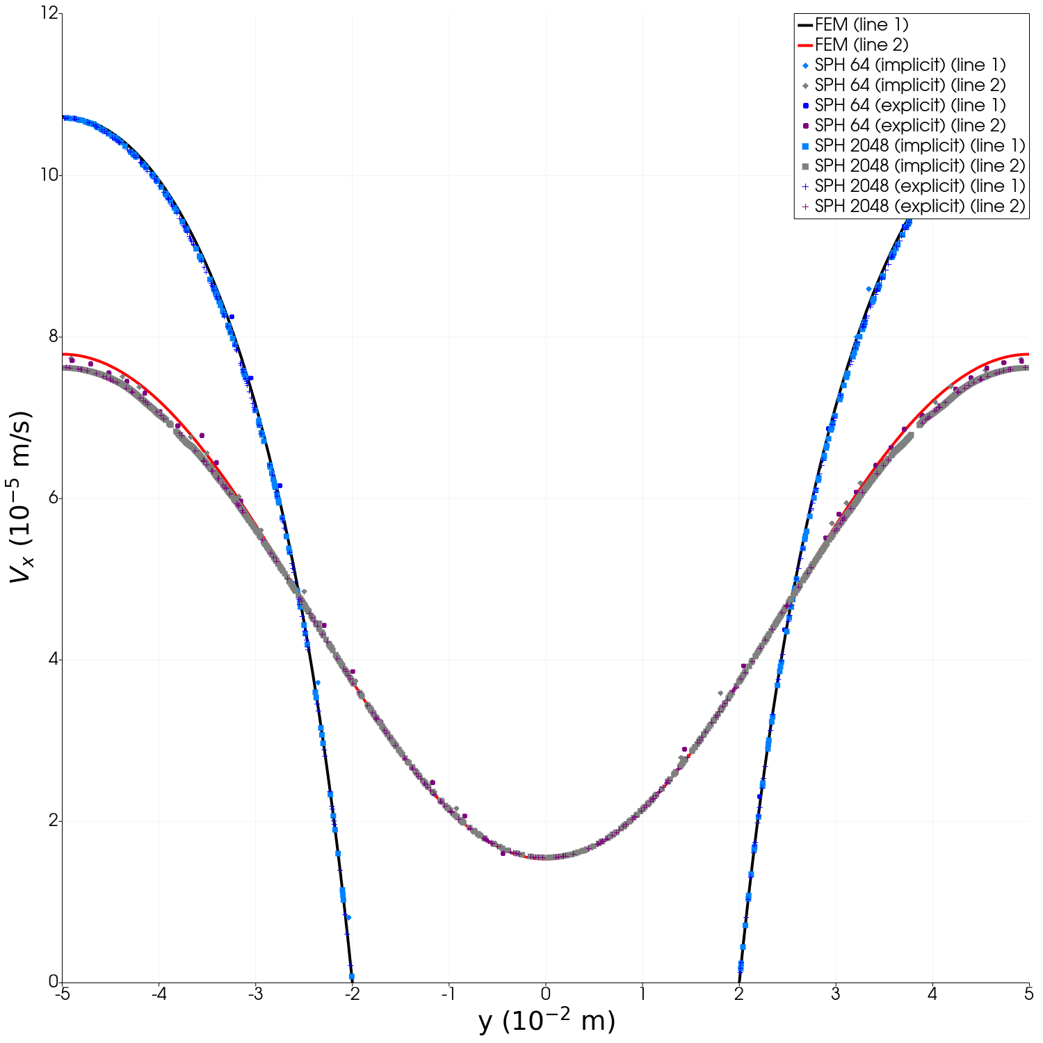
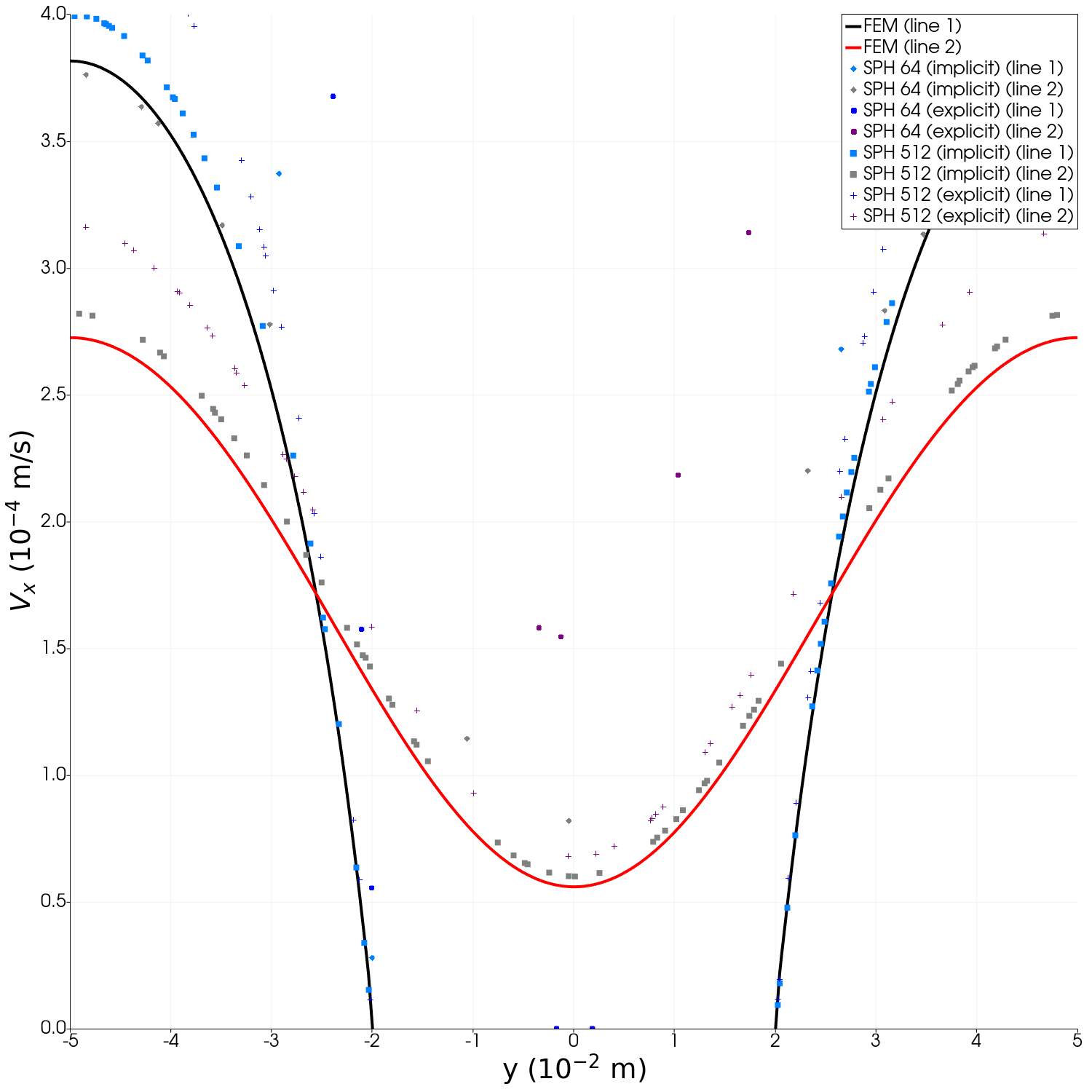
Fig. 12: Velocity along the middle and boundary line for the LRN (left) and VLRN (right) case for the “long” runs, for our semi-implicit integrator at 64 and and a higher p.p.$L$ (SPH) versus the FVE model used for validation. The higher p.p.$L$. is 2048 for the LRN case and 512 for the VLRN.

To validate the model, we compare our results against those obtained using the TRUST code [54], an open source platform developed at the Nuclear Energy Division of the French Atomic Energy Commission (CEA). A Finite Volume Element (FVE) scheme [55, 56] is employed on triangular cells to integrate the Navier–Stokes equations, in conservative form, over the control volumes belonging to the calculation domain [57, 58, 59]. As in the classical Crouzeix–Raviart element, both vector and scalar quantities are located at the centers of the faces. The pressure, however, is located at the vertices and at the center of gravity of a tetrahedral element. This discretization leads to very good pressure/velocity coupling and has a very dense divergence free basis. Along this staggered mesh arrangement, the unknowns, i.e. the vector and scalar values, are expressed using non-conforming linear shape-functions (P1-nonconforming). The shape function for the pressure is constant for the center of the element (P0) and linear for the vertices (P1). The spatial discretization scheme is of second order for both convection and diffusion terms. The time integration scheme is implicit. All linear systems are solved by a direct Cholesky solver. Further information concerning the TRUST code and the numerical methods can be found in [60, 61, 62]. The obtained results are consistent with the ones shown in [31].

Since for this test case we are particularly interested in the effect of particle disorder, we look at the velocity profiles for the ”long” SPH runs, comparing them with the FVE results. We observe that in the LRN case, the semi-implicit and explicit SPH integrators give essentially the same results, and are in good accordance with the FVE results, as shown in both Figure 11 (top row) and 12 (left). The situation is quite different in the VLRN case: the very small timestep in the explicit integrator leads to an accumulation of numerical error that manifests as increasing turbulence and a higher velocity magnitude (Figure 11, bottom row, center column), which reflects in mismatched velocity profiles (Figure 12, right). By contrast, the semi-implicit integrator manages to preserve a good match with the FVE velocity distribution (Figure 11, bottom row, left vs right column), and profiles (Figure 12, right) even in the ”long” run.

6.2 Computational performance

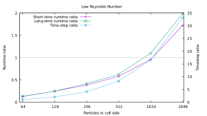
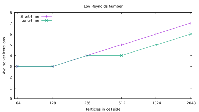
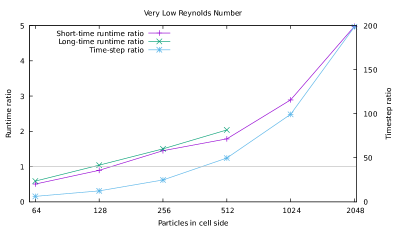
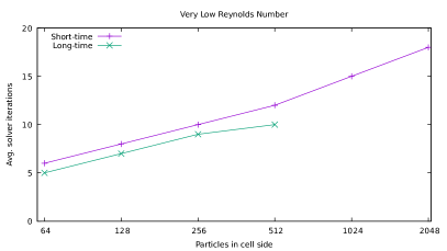
Fig. 13: Left: runtime and timestep ratio between the explicit and semi-implicit integrator. Right: average number of implicit solver iterations (right). Results are for the Low Reynolds Number (top) and Very Low Reynolds Number (bottom) test cases as a function of resolution, for both short and long simulation times.

Consistently with the results presented in [21], the validation of our semi-implicit integration scheme shows a numerical improvement in test-cases where the viscous time-step constraint is dominant and may lead to higher numerical error accumulation in the explicit scheme. Even when the results between the explicit and semi-implicit integration scheme match, however, the semi-implicit scheme can still make a difference in computational performance.

We are particularly interested in seeing if (and how) particle disorder affects the resolution at which it becomes convenient to switch from the explicit to the semi-implicit integrators (“switch-over”). The results are illustrated in Figure 13, where the runtimes for each resolution are taken as the median over three runs (the maximum deviation between the runs is less than $0.5\%$). We show the ratio of the semi-implicit runtime to the explicit runtime, the ratio between the time-step used with the two integrators, and the average number of iterations needed for the solver to converge in the semi-implicit case. “Long” runs for the VLRN case at the higher resolutions are excluded due to the extremely long runtime that would be needed with the explicit integrator.

We remark that particle disorder does not seem to affect the solver convergence negatively: in fact, the average number of solver iterations decreases in the “long” run compared to the early phase (“short” runs). The effect is more visible in the VLRN case than in the LRN case, due to a combination of factors including the difference in physical parameters, the lower number of iterations needed in the LRN even for the “short” run, and the fact that we compute the average number of iterations only up to the nearest integer. The benefit can be seen more clearly in the small improvement in the explicit/semi-implicit runtime ratio for the long run over the short run.

This would not be particularly surprising in an Eulerian framework, since the (Eulerian) velocity remains constant once the steady state is reached. However, in a Lagrangian framework such as SPH, the velocity vector of the particles is not constant even after reaching a steady state, since particles flowing around the cylinder do not move on a straight line: the predictive power of the velocity at the previous time-step as initial guess for the next time-step is thus reduced, although we can see by the reduction in solver iterations that it remains a good choice, and one that is not adversely affected by the increasing particle disorder.

Since the number of solver iterations is a key element in determining the convenience of the semi-implicit over the explicit integrator, in this case the net effect is that in the “long” run the switch-over resolution is coarser than in the “short” run (down to $1024$ p.p.$L$ from $2048$ p.p.$L$ in the LRN case, down to $128$ p.p.$L$ from $256$ p.p.$L$ in the VLRN case).

7 Multi-GPU

A significant advantage of the BiCGSTAB and CG implementations presented here compared to the CG solver used in [21] is the support to parallelize the code across multiple GPUs, either on the same machine or across multiple machines, using the existing GPUSPH infrastructure for this [9, 10].

The key change when distributing the computations across multiple GPUs is the transition from shared-memory parallelism (single GPU) to distributed memory parallelism, and the subsequent need to choose which data to exchange between devices, and when to exchange it. The objective is generally to minimize the number of transfers, minimize the amount of data transferred, and if possible overlap data transfers with computations to (at least partially) cover the data transfer latency. In the implementation we present here, we have aimed to minimize data transfer, but no effort has been made (yet) to overlap computations and data transfers, so we can expect some overhead to be present in the multi-GPU case.

The performance of a multi-GPU implementation can be assessed by looking at strong and weak scaling metrics. Ideal (linear) strong scaling is achieved when running the same problem on $n$ devices takes $1/n$ the time of running on a single device, although in practice this is limited by how much of the program can be parallelized, following Amdahl’s law [63]. Ideal (linear) weak scaling is achieved when running a workload $n$ times larger on $n$ devices takes the same time as running the original workload on a single device [64].

Weak scaling is not always easy to measure, because most workloads are not perfectly linear in the number of particles, so that calibrating the problem size for the tests is frequently non-trivial. We run the multi-GPU tests on the Poiseuille test cases, and for the weak scaling tests we increase the domain size in the periodic cross-flow direction: due to the problem setup, making the domain $n$ times larger gives us exactly $n$ times more particles which —under the assumption that the number of iterations for the implicit solver does not change significantly despite the larger size of the implicit matrix— leads to a linear scaling of the work-load.

The domain size in the cross-flow periodic direction is defined by an aspect parameter $a$, such that the width in the given direction is $aH$ (giving us the original setup for $a=1$). In practice, we observed that the work-load only scales approximately linearly with growing aspect; weak scaling measurements should thus be considered only approximate.

7.1 Cross-device data transfers

In a multi-GPU configuration, a geometric section of the domain is assigned to each GPU; the particles present in the corresponding domain are considered internal to the GPU. Additionally, to allow the device to compute e.g. the forces acting on these particles, each GPU also stores a copy of the particles that are neighbors to the internal particles, but belong to geometrically adjacent devices: these are known as outer edge particles. Finally, we define inner edge particles as particles which are internal to the given GPU, but whose data must be copied to other GPUs (i.e. particles which are “outer edge” for an adjacent GPU).

We can differentiate two classes of computational kernels. If information about neighboring particles is needed (e.g. forces computation), then in a multi-GPU context, each device can only process internal particles, and the data about the outer edge particles must be exchanged; these will be termed internal-only computational kernels. However, if processing of a particle does not require neighbors information (e.g. integration in the explicit scheme), each device can update both its internal particles and the copies of the outer edge particle, avoiding a data exchange; these will be termed in-place computational kernel.

As mentioned in B, we use a Jacobi preconditioner for our solvers. This requires us to compute the diagonal of the (original) matrix during the initialization phase, and since this requires the contributions from the neighbors, each device computes the diagonal entries corresponding to its internal particles, and the inner/outer edge particle data is then exchanged with the adjacent devices.

During the initialization phase, we will also compute and exchange $\mathbf{r}_{0}$ and, for BiCGSTAB, $\hat{\mathbf{r}}_{0}$ which is stored separately (even though it holds the same values as the residual).

During the solver loop, the only vectors that need to be updated across devices are $\mathbf{A}\cdot\mathbf{p}_{k}$ and, in the BiCGSTAB case, $\mathbf{A}\cdot\mathbf{r}\star$, since all other vector updates can be done in-place on each device with the available information.

Steps that require parallel reductions (such as the computation of the residual norm or the updates of the $\alpha,\beta,\gamma,\delta,\omega$ coefficients) will produce partial results on each device, which will then be unified on host to obtain the final result (e.g. by adding up the partial results) and, in the multi-node case, across nodes using MPI primitives.

Due to the very small number of data transfers required during the semi-implicit solver execution, we have provisionally decided to not leverage concurrent transfer and computation, leaving this as a potential optimization opportunity in the future.

7.2 Performance results

We present the result for the Newtonian and Papanastasiou rheology in the plane Poiseuille flow test case, with dummy and dynamic boundary conditions at resolutions of 32 and 64 particles per unit length, and domain aspect from 1 to 4. For each aspect $a$, we test $1$ to $a$ GPUs, resulting in 80 configurations total. To determine the accuracy of the time measurements, we have run each configuration 3 times, resulting in 240 total runs.

We ran the tests on an older machine equipped with 4 NVIDIA GeForce GTX TITAN X (Maxwell architecture, compute capability 5.2): each GPU has 12GB of VRAM an 24 Compute Units (CUs) with 128 “CUDA cores” per CU. The GPUs have peer access (i.e. the possibility to directly access each other’s memory without passing through the host) only in pairs (i.e. device 0 with device 1, and device 2 with device 3), which limits the performance of data exchanges when non-peering devices are involved (and thus in 3- and 4-GPU simulations).

The relative difference between the minimum and maximum runtimes for the 80 configurations is at most $1\%$, with a median of less than $0.1\%$ and a 90th percentile of less than $0.6\%$. Given the stability of the result, we can rely on the median runtime for each configuration in our analysis.

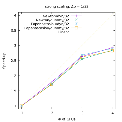
Fig. 14: Strong scaling performance for our multi-GPU implementation, with $\Delta p=1/32$ (left) and $\Delta p=1/64$ (right) with different combinations of rheology and boundary conditions, using the BiCGSTAB solver and the Wendland kernel.

For the strong scaling, we compare the runtime performance of the problems with aspect $a=4$ (figure 14). At the coarser resolution this amounts to about 160,000 particles, while at the finer resolution we have slightly less than 1.2 million particles. The results show close to linear scaling (efficiency between $85\%$ and $96\%$), provided there is enough load: the only case that drops below $85\%$ efficiency is the 4-GPU case with 32 particles per unit length, indicating that in this case there aren’t enough particles (less than 40,000) to fully saturate all devices, despite the large aspect.

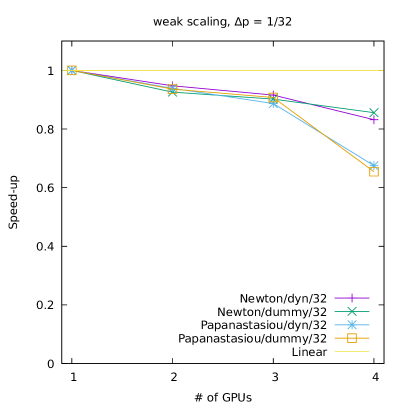
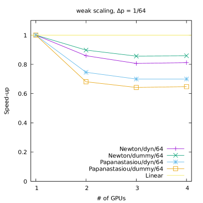
Fig. 15: Weak scaling performance for our multi-GPU implementation, with $\Delta p=1/32$ (left) and $\Delta p=1/64$ (right) with different combinations of rheology and boundary conditions, using the BiCGSTAB solver and the Wendland kernel.

For the weak scaling, we compare the runtime performance of the single-GPU case with aspect $a=1$ with the multi-GPU case where the number of GPUs is equal to the aspect (figure 15). As mentioned before, these results should be considered approximate, since the work-load scaling itself is only being approximately linear as a function of the domain aspect. Still, we get an efficiency of over $80\%$ when using the Newtonian rheology, although the efficiency drops by about $15\%$ in the Papanastasiou case.

The main difference between the two rheologies is the much higher number of implicit solver iterations needed to converge at each time-step (Papanastasiou requiring between 5 and 8 times more iterations than Newton). The lower weak scaling efficiency in this case may thus be indicative of the overhead cost of the data transfers during the solver iterations. Indeed, as mentioned before, we do not overlap computations and data transfers in this case, due to the small number of data transfers needed during each iteration, but as the number of iteration grows, this overhead becomes apparently large enough to measurably affect the runtime.

8 Conclusions and future work

The semi-implicit integration scheme for the viscous term in SPH, introduced in [21], has been extended to support the dummy boundary model, that requires the boundary neighbors viscous velocity to be computed together with the fluid particles. Due to the difference in the expressions for the boundary/fluid contribution versus the fluid/boundary contribution, the resulting coefficient matrix for the implicit system is not strictly diagonally dominant, but the system is still solvable due to it being weakly-chained diagonally dominant.

We adopt a modified version of the biconjugate gradient stabilized method, that is both more robust numerically (particularly important in single precision) and more apt for parallelization in distributed memory configurations (e.g. multi-GPU). Our current multi-GPU implementation achieves very efficient strong scaling (over $85\%$) given a sufficiently large number of particles, although the data transfer overhead has a measurable impact on the weak scaling performance when the implicit solver requires a large number of iterations (typically, for very high values of the viscosity). We expect this to be significantly reduced by introducing striping (overlapping computation and data transfers) in the solver routines.

While the improvements to BiCGSTAB were designed and implemented here in the context of SPH, the numerical and computational benefits of our approach are independent of the numerical method that generates the matrix, and we expect similar benefits in terms of stability and parallelism to be gained in any application adopting BiCGSTAB as a solver.

The computational benefit of the semi-implicit solver over the explicit method in SPH can only be observed at fine resolutions, or when the viscosity is extremely high. Due to the higher cost of the implicit solver, the break-even point for a gain in performance can be estimated at around a factor of $20$ between the time-step restriction for the sound-speed versus the time-step restriction for the viscosity. The actual performance gains are then dependent on the number of iterations needed by the implicit solver. An interesting result that was found is that smoothing kernels with a larger influence radius (and thus a larger average number of neighbors per particle) produce systems that require less solver iterations to converge, partially compensating for the higher computational cost of the kernel evaluation and lowering the break-even point for the convenience of the semi-implicit scheme over the explicit one.

With the availability of a solver that does not require symmetry, further extensions of this approach are possible to other boundary models not explored in this paper (e.g. the semi-analytical boundary models [65]).

A prospective improvement to the approach presented so far would be the adoption of an appropriate preconditioner. This should be fast to compute, and ideally preserve the neighborhood structure of the matrix. While the Jacobi preconditioner we have adopted fits these criteria, its benefits in term of convergence speed are limited.

A better choice for the initial guess may also provide meaningful speed-ups, but the computational cost for more sophisticated alternatives must be taken into consideration, especially in the case of the dummy boundary model, that requires the computation of the initial guess to be split in two separate phases (computation of an initial guess for the fluid particles, followed by the interpolation to produce the initial guess for the boundary particles).

Finally, the good results achieved in the non-Newtonian case indicate that using the viscosity computed from the velocity at the previous time-step is accurate enough to provide superlinear convergence to the theoretical solution, although further improvements can be expected by bringing the computation of the new viscosity into the implicit system. On the other hand, we can expect the resulting non-linearity of the system to have non-trivially higher computational requirements, suggesting the need for a study of the performance/accuracy benefits. Our tests additionally reveal that for shear-dependent viscosity, further tuning to the dummy boundary formulation is necessary to improve the results, and that the excessive numerical dissipation at small smoothing factors and/or influence radius deserves more attention, and may require the need to introduce kernel correction terms in our semi-implicit formulation.

To this end, we are running a more complete set of validation tests, covering all of the several non-Newtonian rheological models currently implemented in GPUSPH and a wider variety of test cases. This is made possible by leveraging the computational benefits of the integrator scheme described here and its particular advantage in the case of non-Newtonian rheologies.

Appendix A Numerical pitfalls in the viscous matrix symmetry

Recall (equations (10) and (15)) that, for fluid particles, the non-zero off-diagonal coefficients of the viscous matrix are

$$a_{\beta\alpha}=\Delta tK_{\alpha\beta}$$

where

$$K_{\alpha\beta}=-\frac{2\bar{\mu}_{\alpha\beta}}{\rho_{\alpha}\rho_{\beta}}F_{\alpha\beta}m_{\alpha};$$

sufficient condition for matrix symmetry is that $m_{\alpha}=m_{\beta}$ (true if all particles have the same mass, numerically), $F_{\alpha\beta}=F_{\beta\alpha}$ and $\bar{\mu}_{\alpha\beta}=\bar{\mu}_{\beta\alpha}$.

The two latter equalities are true analytically. Numerical differences however may arise depending on how the expressions are computed. If the matrix coefficients are not stored, but are computed on-the-fly as in our case, it is also impossible to enforce symmetrization (e.g. by storing the arithmetic mean of $a_{\beta\alpha}$ and $a_{\alpha\beta}$).

This has implications in contexts where the matrix should be symmetric, allowing the use of the conjugate gradient as solver, but ends up not being such numerically, potentially enough to prevent the CG from converging. Our tests have exposed in particular two instances, that we here present, discussing also ways in which they can be prevented.

Fused Multiply-Add

(FMA) is an operation that has been introduced in the 2008 revision of the IEEE-754 standard for floating-point [66]. It takes three arguments $a,b,c$ and computes $a\cdot b+c$ with a single rounding (i.e. as if the product was computed with infinite precision). Modern hardware has good support for this operation, that can be completed in a single cycle, allowing for fast and robust computation of e.g. polynomial in Horner’s form [35]. As pointed out by Kahan [67], FMA is a “mixed blessing”, since improper usage (by either the user or the compiler) can produce issues.

This is exactly the case for the computation of the average viscosity, in some circumstances. Assume for example that the code tracks the kinematic viscosity $\nu$ of the particles, so that the dynamic viscosity is computed as-needed with $\mu=\nu\rho$; assume also that the arithmetic mean is being used as average. Then:

$$2\bar{\mu}_{\alpha\beta}=\nu_{\alpha}\rho_{\alpha}+\nu_{\beta}\rho_{\beta},$$

and with FMA this can be computed using two instructions (a multiplication and an FMA) rather than three (two multiplications and an addition).

However, as Kahan remarks, without further indications there is no way to know if FMA would be used as $\operatorname{fma}(\nu_{\alpha},\rho_{\alpha},\nu_{\beta}\rho_{\beta})$ or the converse (i.e. which multiplication will be fused, and which not). For us, either choice will lead to a non-symmetric matrix, since e.g.

$$2\bar{\mu}_{\alpha\beta}=\operatorname{fma}(\nu_{\alpha},\rho_{\alpha},\nu_{\beta}\rho_{\beta})\neq\operatorname{fma}(\nu_{\beta},\rho_{\beta},\nu_{\alpha}\rho_{\alpha})=2\bar{\mu}_{\beta\alpha}.$$

(and likewise for the other choice of FMA).

In our tests, the compiler may apply this optimization even if $\mu_{\alpha},\mu_{\beta}$ are precomputed. In such circumstances the off-diagonal matrix terms end up with differences in the order of $10^{-8}$, which are sufficient to affect the convergence of the CG (even if not to prevent it altogether). Interestingly, we have only seen this happen for the arithmetic mean; in particular, this does not happen when using the harmonic mean, which is the more physically correct choice of averaging operator with non-uniform viscosity.

A way to avoid this situation is to prevent the compiler from “optimizing” the computation beyond what is allowed by the correct application of the IEEE-754 standard. How to achieve this depends on the specifics of the language and compiler used. In C-based languages, for example, contraction of numerical expressions can be disabled by adding the STDC FP_CONTRACT OFF pragma. Tracking the dynamic viscosity as particle property also avoids this issue altogether, although it may also eliminate other optimization opportunities.

Relative position computation

The computation of $F_{\alpha\beta}$ is symmetric if the computation of $r_{\alpha\beta}$ is symmetric, which is the case if $\mathbf{r}_{\alpha\beta}=\mathbf{r}_{\alpha}-\mathbf{r}_{\beta}$ is computed directly.

This however is not the case when the strategy discussed in [68, 69] is adopted to ensure uniform accuracy throughout the computational domain, which is essential when simulating large domains with fine resolutions, and especially when using single-precision. With the uniform accuracy strategy, the global position $\mathbf{r}_{\alpha}$ of the particle is not stored in the code. Instead, particle positions are tracked as positions $\mathbf{r}^{\prime}_{\alpha}$ relative to the centre of the cells $\mathbf{c}_{\alpha}$ used to speed-up the neighbors search and to split the computation across multiple devices.

Let $\mathbf{l}$ be the vector of the cell side lengths. Then, the distance between two particles can be computed as:

$$\mathbf{r}_{\alpha\beta}=\mathbf{r}^{\prime}_{\alpha}-\mathbf{r}^{\prime}_{\beta}+\mathbf{l}\cdot(\mathbf{c}_{\alpha}-\mathbf{c}_{\beta}).$$

When computing the contributions from all neighbors to a specific particle, it is convenient to pre-compute the offset term $\mathbf{o}_{\alpha\beta}=\mathbf{r}^{\prime}_{\alpha}+\mathbf{l}\cdot(\mathbf{c}_{\alpha}-\mathbf{c}_{\beta})$, which can be used for all neighbors in sharing a cell. However, due to rounding differences, we then have:

$$\mathbf{r}_{\alpha\beta}=\mathbf{o}_{\alpha\beta}-\mathbf{r}^{\prime}_{\beta}\neq\mathbf{r}^{\prime}_{\alpha}-\mathbf{o}_{\beta\alpha}=-\mathbf{r}_{\beta\alpha}.$$

This rounding difference propagates to $F_{\alpha\beta}\neq F_{\beta\alpha}$, ultimately leading to a non-symmetric matrix. In this case, the discrepancies can add up to the point of preventing the CG from converging when it should.

The solution in this case is to only precompute $\mathbf{o}^{\prime}_{\alpha\beta}=\mathbf{l}\cdot(\mathbf{c}_{\alpha}-\mathbf{c}_{\beta})$, and computing the distance as

$$\mathbf{r}_{\alpha\beta}=\mathbf{o}^{\prime}_{\alpha\beta}+(\mathbf{r}^{\prime}_{\alpha}-\mathbf{r}^{\prime}_{\beta}).$$

Grouping the computation of $\mathbf{r}^{\prime}_{\alpha\beta}$ ensures that roundings are done in the same sequence independently from the particle order, resulting in a numerically symmetric matrix, as expected.

Appendix B Implementation notes

We have implemented our own set of Basic Linear Algebra Subprograms (BLAS) routines, covering the essential operations used in the CG and BiCGSTAB algorithms:

axpby

computes $\alpha\mathbf{x}+\beta\mathbf{y}$ for scalars $\alpha,\beta$ and vectors $\mathbf{x},\mathbf{y}$; as an optimization, if a coefficient is zero the corresponding vector is not read from memory; since the condition is uniform (in the parallel sense) and memory access is the primary bottleneck in this operation, this leads to small but measurable performance improvements; the most important benefit of this approach however is that a vector may have undefined content (i.e. not be initialized) if the corresponding coefficient is null, which simplifies the initialization of the CG;

dot product

computes $\mathbf{x}\cdot\mathbf{y}$ for vectors $\mathbf{x},\mathbf{y}$; on GPU this is implemented using the parallel reduction paradigm, with an efficient two-step implementation; additional cross-GPU and cross-node reductions are necessary if more than one GPU or node is being used;

squared norm

i.e. the dot product specialized for the case $\mathbf{y}=\mathbf{x}$, used to compute the norm of $\mathbf{b}$ during initialization, and the norm of $\mathbf{r}_{i+1}$ during the CG iterations;

gemv

computes $\alpha\mathbf{A}\mathbf{x}+\beta\mathbf{y}$ for scalars $\alpha,\beta$, vectors $\mathbf{x},\mathbf{y}$ and matrix $\mathbf{A}$; in our case the matrix is not stored, but expressed as a functional, and our implementation leverages the fact that the structure of $\mathbf{A}$ depends on the neighborhood structure of the underlying SPH method; null coefficients are handled efficiently and robustly also for this operator.

The main reason behind our choice to reimplement the routines rather than relying on existing implementations (such as cuBLAS) is that the additional control on the implementation allows us to tune it for our specific use-cases and existing data structures. This has been particularly important for the axpby and gemv routines, as mentioned.

An additional important aspect of our implementation is that all summations with multiple terms (i.e. the ones in the dot product, squared norms and matrix/vector products) use compensated summation algorithms to improve numerical accuracy, essential due to our use of single precision. In particular, we use the Kahan summation algorithm [70], pending the evaluation of the accuracy/computational cost assessment of the Kahan–Babuška–Neumaier compensated summation [71, 72].

As a bonus, not being tied to existing libraries will reduce migration costs for the adoption of different (i.e. not CUDA) computational technologies.

Storage requirements for CG are of one vector each for $\mathbf{p},\mathbf{r},\mathbf{x}$ and $\mathbf{A}\mathbf{p}$, plus one scalar each for $\gamma_{i}=\mathbf{r}_{i}\cdot\mathbf{r}_{i},\gamma_{i+1},\alpha_{i}$ and $\beta_{i}$. Separate storage of the scalars and vectors takes into account shared/reused sub-expressions as well as the need to hold temporary values for the cross-GPU and cross-node reductions of the dot products and squared norms, but taking into account the possibility to reuse storage (e.g. we can reuse the storage for $\beta_{i}$ to hold $\mathbf{p}_{i}\cdot\mathbf{A}\mathbf{p}_{i}$ after the $\mathbf{p}_{i}$ update and up to the $\alpha_{i}$ computation).

For BiCGSTAB, we need to store two additional vectors compared to CG, $\hat{\mathbf{r}}_{0}$ and $\mathbf{A}\mathbf{r}_{\star}$, and one additional scalar, $\omega$; $\alpha^{\prime}$ and $\alpha$ can share storage, since they are never needed concurrently.

In our experiments, we have further observed an improvement in convergence by adopting a Jacobi preconditioner. This requires two additional computational kernels (one to compute the diagonal terms $\mathbf{D}$ of the matrix, one to divide the right-hand side vector by them), which are executed before the first iteration, and an additional vector to store $\mathbf{D}$ itself, which is needed for all iterations.

For both the CG and BiCGSTAB solver, the initial guess is currently taken to be the solution at the previous time-step. More sophisticated choices are being explored, in an effort to reduce the number of solver iterations necessary to reach convergence.

References

- [1] R. Gingold, J. J. Monaghan, Smoothed particle hydrodynamics : theory and application to non spherical stars, Monthly Notices of the Royal Astronomical Society 181 (1977) 375–389. doi:10.1093/mnras/181.3.375.
- [2] J. J. Monaghan, Smoothed particle hydrodynamics, Annual review of astronomy and astrophysics 30 (1) (1992) 543–574.
- [3] J. J. Monaghan, Smoothed Particle Hydrodynamics, Reports in Progress in Physics 68 (2005). doi:doi:10.1016/j.jcp.2004.08.002.
- [4] D. Violeau, Fluid mechanics and the SPH method: theory and applications, Oxford University Press, 2012.
-
[5]
M. Shadloo, G. Oger, D. Le Touzé,