Fully solvable $n$-dimensional finite simplex lattices with a harmonic spectrum

Fully solvable non-Hermitian finite simplex lattices in arbitrary dimensions

Fully solvable finite simplex lattices with open boundaries in arbitrary dimensions

Abstract

Finite simplex lattice models are used in different branches of science, e.g., in condensed matter physics, when studying frustrated magnetic systems and non-Hermitian localization phenomena; or in chemistry, when describing experiments with mixtures. An $n$-simplex represents the simplest possible polytope in $n$ dimensions, e.g., a line segment, a triangle, and a tetrahedron in one, two, and three dimensions, respectively. In this work, we show that various fully solvable, in general non-Hermitian, $n$-simplex lattice models with open boundaries can be constructed from the high-order field-moments space of quadratic bosonic systems. Namely, we demonstrate that such $n$-simplex lattices can be formed by a dimensional reduction of highly-degenerate iterated polytope chains in $(k>n)$-dimensions, which naturally emerge in the field-moments space. Our findings indicate that the field-moments space of bosonic systems provides a versatile platform for simulating real-space $n$-simplex lattices exhibiting non-Hermitian phenomena, and yield valuable insights into the structure of many-body systems exhibiting similar complexity. Amongst a variety of practical applications, these simplex structures can offer a physical setting for implementing the discrete fractional Fourier transform, an indispensable tool for both quantum and classical signal processing.

I Introduction

Simplex lattice models are used in various fields of science. In physics, they can describe antiferromagnetic Ising models [1, 2, 3] and non-Hermitian localization phenomena [4, 5, 6, 7]. In chemistry, simplex lattices describe blending processes in multi-component systems [8], and in biology, they are used to model arrays of myosin filaments in higher vertebrate muscle packs [9]. A simplex is the simplest possible polytope in a given dimension, such as a line segment, triangle, and tetrahedron in 1D, 2D, and 3D spaces, respectively. Polytopes generalize polyhedra in arbitrary dimensions [10] and have also been widely used in condensed matter physics [11].

Finding the full and exact set of eigenvalues and eigenvectors of finite lattice models in any dimension is a difficult task. While there has been significant progress in finding exact algebraic solutions for certain classes of periodic systems [12, 13, 14, 15, 16], as well as multi-dimensional Hermitian lattices [16], obtaining an analytical expression for the eigenspectrum of finite simplex non-periodic, i.e., with open boundaries, systems remains challenging [17].

Finding new classes of solvable models is also important for benchmarking advanced numerical methods [18, 19]. In addition to their mathematical value, the practical implementation of discovered exactly solvable lattice models in experiments holds significant importance, allowing to gain valuable insights into the nature and behavior of seemingly complex physical systems.

Here we present an analytical solution for the eigenspectrum of finite $n$-simplex lattice models with open boundaries in arbitrary $(n\geq 1)$ dimensions, which, most importantly, can naturally emerge in the field-moments (FMs) space of bosonic systems and, thus, can be immediately simulated with state-of-art experimental setups. In this context, the term open boundaries implies the absence of periodic boundary conditions on such lattices.

At the heart of the proposed solution is the fact that these $n$-simplex lattices can be generated by a dimensional reduction of higher-dimensional iterated polytope chains (IPCs) into low-dimensional iterated simplex chains (ISCs), which are formed in the bosonic FMs space. This space folding can be considered as a special projection of $k$-polytopes on an $n$-dimensional hypersurface, with a subsequent relabeling of the vertex and link weights of a formed lattice. The procedure, thus, echoes the cut-and-project method, used for obtaining quasicrystalline structures from higher-dimensional regular crystals [20, 21, 22, 23, 24], and extends it to non-Hermitian systems. The exact eigenspectrum for the formed $n$-simplex lattices can then be readily attained by exploiting the tensor-product-states character of the eigenfunctions of IPCs.

The present study also generalizes the eigendecomposition of certain tridiagonal matrices [25, 26], used to describe, e.g., angular momentum of quantum light and a number of various photonic non-Hermitian 1D simplex lattices [27, 28]. The findings thus can pave the road to the study of nontrivial non-Hermitian effects in high-dimensional simplex structures.

Our results have potential applications in quantum simulations of non-Hermitian systems. The experimental observation of various many-body phenomena in engineered lattices remains challenging due to the difficulty in controlling all system parameters [29]. Our proposed method offers a promising solution to this problem, as it can be implemented using the FMs space of simple bosonic systems [30]. The FMs space serves as a universal tool, which can provide a broad variety of physical quantities not only in bosonic but also in fermionic systems, ranging from magnetoconductance of electrons to superconducting-normal phase boundaries [31, 32, 33, 34]. That is, the studied $n$-simplex lattices, emerging in the FMs space of quadratic systems, can emulate certain lattice Hamiltonians, allowing for a much simpler, controllable, and scalable quantum simulation of high-dimensional lattices in the synthetic FM space of few-boson systems [35, 36, 37, 38, 39, 40, 41, 42, 43, 44, 45]. The proposed procedure thus opens new avenues for the use of purely Hamiltonian quantum systems, such as linear optical quantum computers [46], for the simulation of nontrivial non-Hermitian phenomena [47].

Furthermore, as a technological application, we show that these simplex lattices, emerging in the FMs space, can also be exploited for implementing the discrete fractional Fourier transform (DFrFT). The DFrFT generalizes the ordinary discrete Fourier transform in a close analogy as the continuous fractional Fourier transform generalizes the continuous ordinary Fourier transform [48]. The DFrFT plays a central role in quantum and classical signal processing [49, 50, 51]. Namely, we demonstrate that these lattice structures can be mapped to the operator space of quantum angular momentum, which is used for implementation of DFrFT [49].

This paper is organized as follows. In Sec. II we elaborate the method for constructing the finite simplex lattices with harmonic spectrum, which naturally appear in the FMs space of quadratic systems. Then, we describe in detail the geometry of these simplex structures and present an exact solution for their eigenspace. In Sec. III, we discuss the potential and significance of the revealed $n$-simplex lattices, highlighting their relevance in both theoretical and practical applications. Conclusions are drawn in Sec. IV.

II The method

To explain the idea of the proposed method for constructing fully solvable harmonic finite simplex lattices, we first consider the specific example of quadratic coupled bosonic modes, where the FMs space gives rise to the IPCs structure. That is, we first study the composition of the evolution matrices governing the dynamics of FMs of this quadratic Markovian system, and then show that the $m$-series of evolution matrices, governing the $i$th-order FMs ($i=1,\dots,m$), can be associated with the corresponding $m$-chain of high-dimensional polytopes, whose highly-degenerate eigenspace is formed by tensor-product-states. Following that, we briefly outline a dimensional reduction procedure of the highly-degenerate space of the IPCs, leading to the formation of exactly solvable ISCs that can emulate real-space $n$-simplex lattices.

II.1 Evolution matrices governing high-order field-moments space

Let us consider a quadratic, in general non-Hermitian, $N$-mode system, whose Hamiltonian is

$$\hat{H}=\sum\limits_{m,n}H_{mn}\hat{\Psi}_{m}^{\dagger}\hat{\Psi}_{n}$$ (1)

with $\hat{\Psi}_{j}$ the $j$th element of the Nambu vector

$$\hat{\Psi}=\left[\hat{a}_{1},\hat{a}_{2},\dots,\hat{a}_{N},\hat{a}_{1}^{\dagger},\hat{a}_{2}^{\dagger},\dots,\hat{a}_{N}^{\dagger}\right]^{T},$$ (2)

where $\hat{a}_{k}$ ($\hat{a}_{k}^{\dagger}$) is the annihilation (creation) operator of the mode $k$, obeying $\left[\hat{a}_{k},\hat{a}_{l}^{\dagger}\right]=\delta_{kl}$ and $\left[\hat{a}_{k},\hat{a}_{l}\right]=0$. From the Heisenberg equations of motion, one can easily write down the equations for the dynamics of the first-order field moments $\langle\hat{\Psi}\rangle$ as

$$\dfrac{{\rm d}}{{\rm d}t}\langle\hat{\Psi}\rangle=M_{1}\langle\hat{\Psi}\rangle,$$ (3)

where $M_{1}$ is the corresponding evolution matrix for the first-order FMs. Note that the same procedure can be straightforwardly extended to Hermitian operators as well to, e.g., bosonic quadrature operators.

The analytical form of an evolution matrix governing the dynamics of any higher-order FMs can be obtained by exploiting properties of matrices formed by Kronecker sums [47]. Namely, any $m$th order FM vector, constructed from the moments of the tensor products of the Nambu vector $\hat{\Psi}$, i.e., ${\Big{\langle}\bigotimes\limits_{1}^{m}\hat{\Psi}\Big{\rangle}}$, is governed by the evolution matrix $M_{m}$, which is obtained from $M_{1}$ as follows

$$\frac{{\rm d}}{{\rm d}t}{\Big{\langle}\bigotimes\limits_{1}^{m}\hat{\Psi}\Big{\rangle}}=M_{m}{\Big{\langle}\bigotimes\limits_{1}^{m}\hat{\Psi}\Big{\rangle}},\quad\text{with}\quad M_{m}=\bigoplus\limits_{1}^{m}M_{1},$$ (4)

where symbols $\bigotimes$ and $\bigoplus$ stand for the Kronecker tensor product and sum, respectively. For more details see Appendix A and Ref. [52]. For simplicity, in Eq. (4), we ignore any possible presence of inhomogeneous parts stemming from quantum noise. Note that for odd-order non-Hermitian FMs, the inhomogeneous part is always absent for weakly coupled Markovian systems, for even-order Hermitian FMs, the noise might enter the r.h.s. of Eq. (4), though it does not affect the frequency spectrum of a system [53].

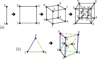
Figure 1: Iterative polytope chains in the field-moments (FMs) space of bosonic (a) dimers and (b) trimers, formed by the Cartesian products of 1-polytope (a line) and 2-polytope (a triangle), respectively. (a) 1-polytope (a line) for the first-order FMs of the dimer; 2-polytope (a square) for its second-order FMs; 3-polytope (a cube) for its third-order FMs, and 4-polytope (a hypercube, shown via its 3D Schlegel diagram) for its fourth-order FMs. (b) 2-polytope (a triangle) for the first-order FMs of the trimer, and 4-polytope (a 4D duoprism, shown via its 3D Schlegel diagram) for its second-order FMs. Numbered vertices correspond to the elements of the FMs vector ${\langle\bigotimes^{k}_{1}\hat{\Psi}\rangle}$, with vertex potentials and the link weights corresponding to the diagonal and off-diagonal elements of the related evolution matrix $M_{k}$, respectively.

Figure 2: Tensor-products tree of the eigenvectors of the evolution matrices $M_{m}$ (with $m=0,1,2,3$) for a quadratic dimer, according to Eq. (6). The index $m=0$ corresponds to the identity element. This tree is a solution for the iterative polytope chains in Fig. 1(a).

II.2 Iterated polytope chains in the field-moments space of bosonic systems

A chain of $m$ evolution matrices $M_{1}\to M_{2}\to\dots\to M_{m}$, in Eq. (4), induces an IPC of $m$ $i_{k}$-polytopes,

$$P_{i_{1}}\to P_{i_{2}}\to\dots\to P_{i_{m}},$$ (5)

produced by iterated Cartesian powers of $P_{i_{1}}$; namely,

$$P_{i_{k}}=\left(P_{i_{1}}\right)^{k},$$

where $P_{i_{1}}$ is actually a simplex, i.e., the simplest polytope in a given dimension associated with the first-order FMs space.

The dimension of a polytope $P_{i_{k}}$ is $k\times d$, where $d$ is the dimension of the $P_{i_{1}}$ polytope. The vertices of a polytope $P_{i_{k}}$ are given by the elements of the FMs vector ${\langle\bigotimes^{k}_{1}\hat{\Psi}\rangle}$. The vertex potentials and link weights are determined by the diagonal and off-diagonal elements of the matrix $M_{k}$, respectively. Moreover, because the matrix $M_{k}$ inherits the symmetry of $M_{1}$, according to Eq. (4), the links in $P_{i_{k}}$ preserve the symmetry of those in the polytope $P_{i_{1}}$. Note that, in general, the polytope links can be asymmetric, i.e., with two different weights in opposite directions, if the FMs evolution matrices are non-symmetric.

For instance, in case of a symmetric bosonic dimer, an evolution matrix $M_{1}$ can be associated with a 1D polytope $P_{1}$, i.e., a line, formed by two vertices and one edge [see Fig. 1(a)]. A 2-polytope $P_{2}$, corresponding to $M_{2}$, then represents a square. As a result, one obtains an $m$-hypercube, describing the $m$th-order FMs space, whose associated matrix is $M_{m}$ [see Fig. 1(a)]. Figure 1(b) illustrates the first two polytopes corresponding to the first and second-order FMs of a symmetric three-mode system.

II.3 Tensor product eigenspace for iterated polytope chains

Here we discuss the eigenspace of the evolution matrices $M_{m}$ associated with IPCs. Equation (4) implies that one can determine a complete eigendecomposition of the matrix $M_{m}$, governing $m$th-order FMs, knowing the eigenvalues and eigenvectors of the matrix $M_{1}$, and, therefore, the eigenspace of corresponding $i_{m}$-polytope (see Fig. 2 and Appendix A for details). Namely, the eigenvectors of the matrix $M_{m}$ are found via all $(2N)^{m}$ combinations of the tensor products of the eigenvectors $\psi_{j}^{(1)}$, $j=1,\dots,2N$ of the matrix $M_{1}$, together with the harmonic eigenvalues:

$$\psi^{(m)}_{i_{1},i_{2},\dots,i_{m}}=\psi_{i_{1}}^{(1)}\otimes\dots\otimes\psi_{i_{m}}^{(1)},\quad\lambda^{(m)}_{i_{1},i_{2},\dots,i_{m}}=\sum\limits_{k=1}^{m}\lambda_{i_{k}}^{(1)},$$ (6)

where each index $i_{k}=1,\dots,2N$, for each $k=1,\dots,m$, and $\lambda^{(1)}_{i_{k}}$ are the eigenvalues of the matrix $M_{1}$ (see Appendix A).

The expression in Eq. (6) implies that the FMs space, associated with IPCs, can exhibit a large extra algebraic (diabolic) degeneracy, which is rapidly increasing with the FMs order. In all subsequent discussions, unless stated otherwise, we will call algebraic degeneracy the extra degeneracy linked with the construction of the IPCs. We will not refer to the other types of algebraic degeneracies, including those which are intrinsically associated with the spectrum of the generating matrix $M_{1}$. The akgebraic degeneracy stems from the fact that the different combinations of the eigenvalues $\lambda_{i_{k}}$ may result in the same sum in Eq. (6), but correspond to different eigenvectors. One can then straightforwardly calculate the algebraic degeneracy $D$ for a given eigenvalue $\lambda^{(m)}_{i_{1},i_{2},\dots,i_{m}}$, as

$$D(\lambda^{(m)}_{i_{1},i_{2},\dots,i_{m}})=\dfrac{m!}{{n_{i_{1}}!n_{i_{2}}!\dots n_{i_{m}}!}}$$ (7)

where $n_{i_{k}}$ denotes the number of times the index $i_{k}$ appears in Eq. (6).

Noticeably, this diabolic degeneracy, originating in the IPCs eigenspace, can lead to a nontrivial interplay between diabolic points and exceptional points [54], provided that an evolution matrix $M_{1}$ possesses the latter. This can result in the formation of hybrid diabolically-degenerate exceptional points (see Appendix C for details and also Ref. [53]). And while it may be challenging to directly access and utilize the properties of such hybrid degeneracies in the FMs space, they can be engineered and probed with a relative ease in the spectrum of real-space systems exhibiting unique dynamical features [55].

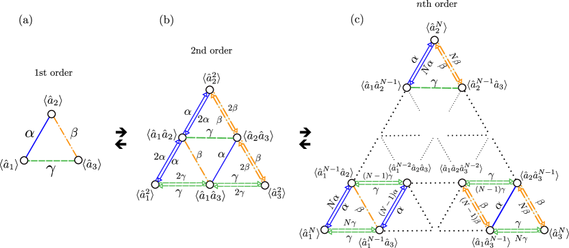
Figure 3: Formation of iterative simplex chains (ISCs) by folding iterative polytope chains in the field-moments (FMs) space of bosonic three-mode systems. (a) A 2-simplex, i.e., a triangle, formed in the first-order FMs, which coincides with the $P_{i_{1}}$ polytope. The links, denoted by $\alpha,\beta,\gamma$ of different colors, correspond to the coupling strengths between the three FMs, according to Eq. (10). (b) ISC in the second-order FMs space. By folding the corresponding symmetric $4$-polytope in Fig. 1(b), one arrives at an asymmetric triangular 2-simplex consisting of six vertices, according to Eq. (8). (c) ISC in the $N$th-order FMs space. The ISCs, thus, form a finite triangular non-Hermitian lattice with $(N+1)(N+2)/2$ vertices in the high-order FMs space. Formally, the presented 2-simplex chain can be considered in a reversed order, that is, a lattice in panel (c) can be reduced into a lattice in panel (a), which highlights the simple origin of the seemingly complex lattice in (c). Note that such formed asymmetric simplex lattices in the FMS of quadratic bosonic systems can be additionally symmetrized (see Appendix E for details).

II.4 Dimensional reduction of iterated polytope chains to iterated simplex chains, and the formation of finite simplex lattices

As mentioned above, the extra algebraic degenerate space in IPCs stems from the tensor-product-states nature of the FM vectors ${\langle\bigotimes^{m}_{1}\hat{\Psi}\rangle}$. Indeed, in a simple case of a linear dimer consisting of interacting fields, described by $\hat{a}_{1}$ and $\hat{a}_{2}$, the system dynamics for the FMs $\langle\hat{a}_{1}\hat{a}_{2}\rangle$ and $\langle\hat{a}_{2}\hat{a}_{1}\rangle$ is the same, though both these moments appear in the FMs vector ${\langle\bigotimes^{2}\hat{\Psi}\rangle}$ by construction. However, one can effectively eliminate this redundant degeneracy by reducing $(2N)^{m}\times(2N)^{m}$-dimensional evolution matrices $M_{m}$, describing $k_{m}$-polytopes, to low-dimensional effective matrices $M_{m}^{\rm eff}$ of the size

$$S_{m}(2N)=\dfrac{(2N+m-1)!}{m!(2N-1)!}<(2N)^{m}.$$ (8)

The expression for $S_{m}$ is the standard formula for combinations with repetition, which leaves only non-equivalent FMs in the description of the FMs time evolution.

The projection of the matrix $M_{m}$ onto $M_{m}^{\rm eff}$ can be generally represented as

$$M_{m}^{\rm eff}=TL^{\dagger}M_{m}RT^{-1},$$ (9)

where $L$ and $R$ are $(2N)^{m}\times S_{m}(2N)$ rectangular matrices comprised by the left and right eigenvectors of the matrix $M_{m}$, respectively. They project the matrix $M_{m}$ onto its low $S_{m}$-dimensional non-degenerate eigenspace, and where $T$ is a $S_{m}\times S_{m}$ similarity transformation, e.g., a rotation, which allows to write down $M_{m}^{\rm eff}$ in an arbitrary basis (see Appendix B for more details). Since the eigenspace of the matrix $M_{m}$ can be readily calculated in Eq. (6), one then immediately obtains the eigenspace of the reduced matrix $M_{m}^{\rm eff}$.

Interestingly, the series of effective evolution matrices

$$M_{1}^{\rm eff}\to M_{2}^{\rm eff}\to\dots\to M_{m}^{\rm eff}$$

can now be associated with an ISC, in analogy with Eq. (5). In other words, the dimensional reduction of evolution matrices $M\to M_{\rm eff}$ is accompanied by the space reduction of the corresponding IPC into ISC. Moreover, such ISCs are defined in the same dimensional space as the simplex (polytope) $P_{1}$.

Recall that for the first-order FMs, the polytope $P_{1}$ is actually a simplex. For instance, for a dimer, whose 1-simplex $P_{1}$ is a 1D line segment [see Fig. 1(a)], its ISC defines a line consisting of $[S_{m}(2)=m+1]$ vertices in the reduced $m$th-order FMs space. Accordingly, for a trimer, with $P_{1}$ being a triangle, i.e., a 2-simplex, [Fig. 1(b)], the ISC defines a triangular chain on 2D plane (see Fig. 3). Similarly, the high-order FMs space of an $n$-mode system can be represented by $(n-1)$-simplex chains.

This space reduction of IPCs into ISCs can formally be considered as a projection of $k_{m}$-polytopes onto an $(n-1)$-dimensional hypersurface which is formed by $n$ points corresponding to the $m$th order of $n$ fields, i.e., $\langle\hat{a}_{1}^{m}\rangle,\langle\hat{a}_{2}^{m}\rangle\dots,\langle\hat{a}_{n}^{m}\rangle$. After such a projection, a $k_{m}$-polytope is folded into a $(n-1)$-simplex lattice with $S_{m}(n)$ vertices. The vertex and link weights of the formed simplex lattice are then assigned by the corresponding effective matrix $M_{m}^{\rm eff}$. For instance, for a dimer, the 1D-hypersurface (a line) is the main diagonal of the $(k_{m}=m)$-hypercube formed by two ‘vertices’ $\langle\hat{a}_{1}^{m}\rangle$ and $\langle\hat{a}_{2}^{m}\rangle$. As such, $2^{m}$ vertices of a $m$-cube are projected to a $S_{m}(2)=(m+1)$ vertices lying on the main diagonal with the vertex and link weights described by the effective matrix $M_{m}^{\rm eff}$.

Importantly, the reduction of IPCs into ISCs results in the formation of finite $n$-simplex lattices which do not possess translational symmetry, regardless whether the underlying and generating matrix $M_{1}$ is symmetric or not (see also Sec. II.5). This also implies that these constructed simplex structures can only describe finite lattices with open boundaries, because no periodic conditions can be imposed. The latter restriction evidently stems from the requirement that these lattices have a harmonic spectrum.

The finite lattices, emerging in the FMs space of quadratic bosonic systems, can additionally emulate various real-space and other synthetic lattice models described by (non-) Hermitian Hamiltonians, whose matrix representation is equivalent to some $M_{m}^{\rm eff}$. Meaning that a high-order FMs space of bosonic systems can be used to find exact solutions of various finite (non-) Hermitian lattice models in arbitrary dimensions. In other words, if the geometry of an arbitrary Hamiltonian, which can be expressed via a n-simplex lattice (in a real or synthetic space), can be identified with that of the constructed simplex structures studied here (see Sec. II.5 and Appendix D for typical examples), one can then readily obtain its exact eigenspectrum. This observation constitutes one of the main results of our work. Note, however, that the state spaces and the physical meaning of the state vectors can substantially differ depending on the representation of the emulated Hamiltonian. In Sec. III, we additionally discuss the practical relevance and other potential physical scenarios, where these $n$-simplex lattices can occur and be effectively utilized.

II.5 Example: Exactly solvable finite triangular non-Hermitian lattices with open boundaries

To elaborate more on the above described procedure of obtaining finite simplex lattices with open boundaries in the FMs space, as an example, let us consider a linear three-mode system. Assume that its first-order FMs vector $\langle\hat{\Phi}\rangle$, $\hat{\Phi}=[\hat{a}_{1},\hat{a}_{2},\hat{a}_{3}]^{T}$, is governed by the following symmetric evolution matrix [see also Fig. 3(a)]:

$$M_{1}=\begin{pmatrix}0&\alpha&\gamma\\ \alpha&0&\beta\\ \gamma&\beta&0\end{pmatrix}.$$ (10)

The diagonal elements of $M_{1}$ can be in general complex-valued. The evolution matrix $M_{N}$, governing the dynamics of the $N$th-order FMs vector ${\langle\bigotimes^{N}_{1}\hat{\Phi}\rangle}$, is then obtained from $M_{1}$ according to Eq. (4). The $M_{N}$ describes a highly degenerate $2N$-polytope [the case for $N=1,2$ is shown in Fig. 1(b)]. This redundant degeneracy can be eliminated via the map $M_{N}\to M_{N}^{\rm eff}$, which geometrically corresponds to the reduction of a symmetric $2N$-polytope, with $3^{N}$ vertices, to a 2D ISC forming a finite non-Hermitian triangular lattice with

$$S_{N}(3)=(N+1)(N+2)/2$$

vertices (see Fig. 3). The non-Hermitian nature of such a formed lattice is highlighted by the arising asymmetry in vertex bonds which become direction-dependent.

One can see in Fig. 3 that by iteratively increasing the FMs order, the corresponding ISC are iteratively augmented by 2-simplexes, (i.e., triangles), generating thus a triangular lattice. This emerging triangular lattice can mimic a real-space bosonic non-Hermitian Hamiltonian $M_{N}^{\rm eff}\to H_{\rm eff}^{N}$ written in a mode representation. We give an explicit expression for this Hamiltonian in Appendix D. Importantly, this triangular lattice model in Fig. 3(c) is exactly solvable, since the eigenspace of the matrix $M_{N}^{\rm eff}$ is readily obtained from $M_{N}$ in Eq. (6) by applying the described projection.

Similarly, as was mentioned earlier, a $m$-dimensional hypercube, related to the $m$th-order FMs of a dimer, can be reduced to a 1D non-Hermitian chain [depicted as one of the external boundaries of the triangular lattice in Fig. 3(c)] which is described by a tridiagonal Sylvester matrix $M_{k}^{\rm eff}$ [28]. Moreover, for a four-mode system one attains a tetrahedral-octahedral honeycomb lattice (see Appendix D). It is straightforward to extend this procedure to arbitrary $n$-mode systems, whose FMs space can be described by the corresponding $(n-1)$-simplex lattices with open boundaries.

Note that one can try to symmetrize a non-Hermitian matrix $M_{m}^{\rm eff}$ by choosing an appropriate basis if any. For example, for a 2-simplex lattice, shown in Fig. 3, one can find such a basis where the corresponding reduced matrix $M_{m}^{\rm eff}$ becomes symmetric (see also Appendix E for details).

This analysis can also be straightforwardly extended to any kind of a (non-) Hermitian matrix, which defines the evolution of the first-order field moments (away from exceptional points [56]). As the simplex lattices are characterized by the bidirectional couplings, the asymmetry in $M_{1}$ is simply reflected in the modification of the corresponding link weights. For instance, by modifying the single element $M_{1}(1,2)=\eta$ in Eq. (10), (i.e., changing only the tunneling amplitude from the mode $\hat{a}_{1}$ to the mode $\hat{a}_{2}$ ), the weights of links, denoted by the blue-colored vectors at $45^{\circ}$ in panels (b) and (c) of Fig. 3, become factorized by the new parameter $\eta$. The remaining link weights remain unchanged. The symmetry of the underlying matrix $M_{1}$, which is explicitly reflected in its spectrum, then persists in any subsequent matrix $M_{m}^{\rm eff}$, and, therefore, in the associated $n$-simplex structures. The latter property follows from the harmonic character of the spectrum of $M_{m}^{\rm eff}$, constructed by the eigenvalues of $M_{1}$. For instance, if the matrix $M_{1}$ possesses the chiral or parity-time ($\cal PT$) symmetry, that symmetry is also present in the formed $n$-simplex lattices.

III Applications

III.1 Discrete fractional Fourier transform

Here we show that 1D simplexes provide a physical setting for the computation of the DFrFT in the FMs space of a photonic symmetric dimer. As it has been already demonstrated in Ref. [49], by mapping the matrix of the angular momentum operator $J_{x}$ onto a real-space Hamiltonian, describing the 1D array of coupled waveguides, one can effectively implement the DFrFT of any input signal. Our goal here is to show that the effective matrix $M_{N}^{\rm eff}$, which determines the evolution of the $N$th-order FMs space of the symmetric dimer and is associated with a synthetic finite 1-simplex array, can be cast onto the $J_{x}$ matrix.

Geometrically, this 1-simplex array can be represented as one of the three main outer sides of the 2D simplex in Fig. 3(c), e.g., by the outer left-hand-side of the lattice, where the link weights factored by the parameter $\alpha$. This 1D-chain of the 2D simplex describes the FMs interaction between the modes $\hat{a}_{1}$ and $\hat{a}_{2}$, while eliminating the presence of the mode $\hat{a}_{3}$ [see Fig. 3(c)]. The elements of the $(N+1)\times(N+1)$ FMs evolution matrix $M_{N}^{\rm eff}$ then has the following Sylvester tridiagonal form [26, 47] (see also Appendix C):

$$M_{N}^{\rm eff}(j,k)= (N-j)\alpha\delta_{j,k-1}+j\alpha\delta_{j,k+1},$$ (11)

with indices $j,k=0,\dots,N$. The matrix $M_{N}^{\rm eff}$ can be transformed into the operator of the quantum angular momentum (up to a scaling factor 2$\alpha$) via a similarity transformation:

$$J_{x}=S^{-1}M^{\rm eff}_{N}S,$$ (12)

where the diagonal matrix $S$ reads (see Appendix E)

$$S(j,j)=\prod\limits_{k=1}^{j}\sqrt{\frac{M_{N}^{\rm eff}(k,k-1)}{M_{N}^{\rm eff}(k-1,k)}},$$ (13)

with $S(0,0)=1$. The matrix $J_{x}$ has the form

$$J_{x}(m,n)= {\alpha}\Big{[}\sqrt{(j-m)(j+m+1)}\delta_{m+1,n}$$ (14)

$$+\sqrt{(j+m)(j-m+1)}\delta_{m-1,n}\Big{]}.$$

For simplicity, we keep the $(N+1)\times(N+1)$ matrix $J_{x}$ in the standard form, where the indices $m$ and $n$ range from $-j$ to $j$ in unit steps, and $N=2j$. The parameter $j$ is a positive integer or half-integer. Thus, the 1D simplex lattice, arising in the FMs space of a symmetric dimer, becomes similar to the operator space of the quantum angular momentum.

One of the outcomes, stemming from the above correspondence, is the ability to compute the DFrFT of real-space 1D signals in the synthetic FMs space of the dimer. This can be achieved, for instance, by appropriately preparing the initial quantum state of a dimer, whose input vector of the field moments can then emulate a given 1D real-space signal. Such a task can be achieved in quantum hardware through quantum optimal control algorithms, such as, e.g., GRAPE [57] or CRAB [58] algorithms, Most importantly, since the FMs space are robust against any perturbations by construction, it makes the computation of DFrFT resilient to additional noise, which inevitably arises due to experimental imperfections when engineering 1D arrays in real space [49]. As the further step of our study, it would be interesting to examine the potential of the revealed harmonic $n$-simplex lattices to serve as a general framework for implementing the DFrFT in arbitrary dimensions for any $n>1$.

We note that the isomorphism between the angular momentum operators and bosonic creation and annihilation operators of two-mode systems is known in the literature by exploiting the Jordan-Schwinger transformations from which one can recover the same operator Lie algebra [59]. Here, however, and quite remarkably, we have unveiled the same angular momentum-bosonic dimer correspondence without any references to the system operators defined on the Fock Hilbert space, dealing exclusively with the geometry of $c$-number-valued FMs. Moreover, we extend this correspondence to arbitrary $m$-mode quadratic systems (see Appendix E for details). This also means that experimental simulations of angular momenta can also be directly implemented in the FMs space of a dimer without relying, e.g., on postselection procedures, which directly exploit the Jordan-Schwinger transformations in the photon-number space of the system operators [60], and which, therefore, are hard to realize in practice for many-photon systems.

III.2 Other applications

The possibility to engineer chiral and $\cal PT$-symmetric $n$-simplex structures also enable to study various topological, localization, and order-disorder transition phenomena in high dimensions. Thanks to their harmonic spectrum, one can easily engineer high-dimensional simplex lattices with, e.g., exceptional points or even hybrid diabolically-degenerate exceptional points [55] of an arbitrary degeneracy. It is well known that the presence of highly-degenerate exceptional points may induce various non-Hermitian phase transitions [6, 61]. In particular, in Ref. [28] we have already unveiled the emergence of the non-Hermitian skin effect in the synthetic space of a $\cal PT$-symmetric dimer, whose FMs space corresponds to the 1-simplex array. The latter observation thus necessitates a further study of the associated non-Hermitian phenomena which can occur in high-dimensional $n$-simplex lattices for arbitrary large $n>1$.

We note that compared to Ref. [28], here we explicitly give the recipe for the construction of arbitrary dimensional $n$-simplex lattices in the FMs space, and, moreover, we found a general solution for their eigendecomposition. In particular, we present an alternative spectral solution for tridiagonal Sylvester matrices, whose exact eigenspectrum has been obtained only recently [26]. Therefore, we believe that our findings could also motivate and be of interest for future research in related mathematical and theoretical fields.

Besides the described possible theoretical and experimental applications of the given $n$-simplex lattices, primarily, they offer a simple visual representation and give valuable insights into the structure of the FMs space of bosonic quadratic systems. This result, to the best of our knowledge, was not previously known. Additionally, the exact eigendecomposition of these simplex structures provides an alternative solution for the high-order FMs of quadratic systems, thus bypassing the need to invoke the Wick theorem [62].

IV Conclusions

We have revealed the formation of nontrivial exactly solvable non-Hermitian harmonic finite lattice models with open boundaries in the FMs space of arbitrary quadratic bosonic $n$-mode systems. The spectrum of such lattices, represented by ISCs, can be readily obtained by knowing the spectrum of higher-dimensional matrices describing IPCs, which are much easier to compute by exploiting the simple eigenspace structure of the latter.

Our results extend and generalize the previous works in Refs.  [25, 26, 28], and provide valuable insights into the underlying structure of many-body lattice systems exhibiting similar complexity. These findings can prompt further studies on simulation of various high-dimensional lattice topological and localization phenomena in the FMs of multimode bosonic systems. The results can also be directly utilized for finding high-order FMs of quadratic systems even without invoking the Wick theorem.

One of our main observations in this study is that some lattice structures, which look complex at first sight, can originate from simple low-dimensional arrangements. This insight, thus, resonates with the concept of quasicrystalline structures, which can be obtained through the projection of high-dimensional regular crystals onto certain hyperplanes [63], or can even draw parallels with fractal-like formations, where complex geometric patterns arise from much simpler geometric objects via iterative transformations [64].

These findings also enable a potential application of $n$-simplex lattices to provide a physical setting for realizing an arbitrary dimensional DFrFT either directly in the synthetic FMs space or in real space. This can pave the way for numerous intriguing applications in integrated quantum computation and various information processing tasks.

The last but not least, the revealed here exotic hybrid spectral features, namely, emerging diabolically degenerate exceptional points in the unfolded bosonic FMs space, can be motivating for constructing real-space Hamiltonians describing multimode systems with unique dynamical characteristics [55].

Appendix A Tensor product states in the higher-order field moments dynamics of quadratic systems: Kronecker products and sums

In this section we detail on the construction of the evolution matrices for higher-order FMs based on the Kronecker sum operations and their eigendecomposition.

As we have already stressed, one of the remarkable features of quadratic systems is that one can obtain the analytical form of an evolution matrix ruling the dynamics of any higher-order FMs from the form of the evolution matrix $M_{1}$ for the first-order FMs in Eq. (4). This can be done by exploiting some properties of matrices formed by Kronecker sums. First, we summarize the most important spectral features of Kronecker sum matrices in the following theorem.

Theorem 1.

Theorem. The eigenspectrum of a complex matrix $C\in{\mathbb{C}}^{(m+n)\times(m+n)}$, obtained as the Kronecker sum of two complex matrices $A\in{\mathbb{C}^{m\times m}}$ and $B\in{\mathbb{C}^{n\times n}}$, i.e., $C=A\oplus B=A\otimes I_{B}+I_{A}\otimes B$, has the form

$$\lambda(C)=\lambda(A)+\lambda(B),\quad\psi_{C}=\psi_{A}\otimes\psi_{B},$$ (15)

where $\lambda(M)$ and $\psi_{M}$ are the eigenvalues and eigenvectors of a matrix $M=A,B,C$, respectively.

Proof.

The proof is straightforward. We start from the eigenvalue-eigenvector equation for the matrix $C$, by feeding it into the equation for the right eigenvector, which is a tensor product of the two eigenvectors $\psi_{A}$ and $\psi_{B}$, with eigenvalues $\lambda(A)$ and $\lambda(B)$, respectively. Namely,

$$C(\psi_{A}\otimes \psi_{B})=(A\oplus B)$$ (16)

$$=(A\otimes I_{B})(\psi_{A}\otimes\psi_{B})+(I_{A}\otimes B)(\psi_{A}\otimes\psi_{B})$$

$$=(A\psi_{A}\otimes I_{B}\psi_{B})+(I_{A}\psi_{A}\otimes B\psi_{B})$$

$$=(\lambda_{A}\psi_{A}\otimes\psi_{B})+(\psi_{A}\otimes\lambda_{B}\psi_{B})$$

$$=(\lambda_{A}+\lambda_{B})\psi_{A}\otimes\psi_{B},$$

where we used the tensor and dot product properties of matrices and vectors. In other words, the eigenvector of the matrix $C=A\oplus B$, corresponding to the eigenvalue $\lambda(C)$, is indeed just the tensor product of the two eigenvectors of the matrices $A$ and $B$ with eigenvalues $\lambda(A)$ and $\lambda(B)$. ∎

According to Eq. (16), the matrix, whose eigenvectors are formed by the tensor products of eigenvectors of two matrices can be utilized in the construction of the evolution matrices of any higher order. To reveal how this works in practice, let us consider the second-order field moments. The various combinations of second-order field moments are obtained from the tensor product of the Nambu vector,

$$\hat{\Psi}=\left[\hat{a}_{1},\hat{a}_{2},\dots,\hat{a}_{N},\hat{a}_{1}^{\dagger},\hat{a}_{2}^{\dagger},\dots,\hat{a}_{N}^{\dagger}\right]^{T},$$ (17)

on itself, i.e., from the $4N^{2}$ dimensional vector $\langle\hat{\Psi}\otimes\Psi\rangle$. According to Eq. (16), the evolution matrix $M_{2}$, governing the vector of the second-order FMs,

$$\frac{{\rm d}}{{\rm d}t}\langle\hat{\Psi}\otimes\Psi\rangle=M_{2}\langle\hat{\Psi}\otimes\hat{\Psi}\rangle,$$ (18)

attains the form

$$M_{2}=M_{1}\oplus M_{1}=M_{1}\otimes I_{2N}+I_{2N}\otimes M_{1}.$$ (19)

The form of the evolution matrix $M_{2}$ coincides, as it should, with that derived from the Lyapunov equation for the covariance matrix, when the latter is presented as a column vector [52]. This procedure can, thus, be iteratively continued to any $m$th order field moment vectors ${\Big{\langle}\bigotimes\limits_{1}^{m}\Psi\Big{\rangle}}$, thus obtaining Eq. (4).

The eigenvectors space for such evolution matrices $M_{m}$ governing $m$th-order FMs can be, thus, represented as a tree structure, according to Eq. (6). For instance, for a dimer, this tree structure takes the form shown in Fig. 3.

Appendix B Dimensional reduction of polytopes to simplexes in the field-moments space of bosonic systems

As we have already stressed, the highly-degenerate eigenspace of a $(2N)^{m}\times(2N)^{m}$ matrix $M_{m}$ can be effectively reduced to the non-degenerate space of a matrix $M_{m}^{\rm eff}$ of size $S_{m}(2N)\times S_{m}(2N)$. This space folding can be associated with the dimensional reduction of a polytope to a simplex. The reduction of the degenerate space can be performed in accordance with the following algorithm, which allows to simultaneously retrieve both the reduced matrix $M_{m}^{\rm eff}$ and its eigenvectors.

• Define $(2N)^{m}\times(2N)^{m}$ matrices $A$ and $B$, which consist of all the eigenvectors of $M_{m}$ and basis vectors $v_{k}=[0,\dots,1_{k},\dots,0]^{T}$, respectively: $A=[\psi_{1},\dots,\psi_{m}]$, and $B=[v_{1},\dots,v_{m}]$. The matrix $B$, thus, can be chosen as the identity matrix.

• Eliminate all extra degenerate eigenvectors in $A$ corresponding to a $D_{i}$-fold eigenvalue $\lambda_{i}$, such that among all the degenerate eigenmodes $\psi^{(N)}_{i_{1},i_{2},\dots,i_{N}}$ only one representative eigenvector

  $$\psi^{m}(\lambda_{i})=\dfrac{1}{D_{i}}\sum\limits^{D_{i}}\psi^{(N)}_{i_{1},i_{2},\dots,i_{N}}$$ (20)

  is left in the matrix. This transforms $A$ to a matrix $A^{\prime}$ of the size $(2N)^{m}\times S_{m}$, which determines the non-degenerate eigenspace of $M_{m}$ one wants to project on.

• Repeat the same procedure for the matrix $B\to B^{\prime}$, collecting and eliminating the columns with the same indices as in the map $A\to A^{\prime}$. Matrix $B^{\prime}$ defines the basis for the reduced matrix $M_{m}^{\rm eff}$.

• Project the $(2N)^{m}\times(2N)^{m}$ matrix $M_{m}$ onto its non-degenerate $S_{m}(2N)$-dimensional eigenspace spanned by the columns in $A^{\prime}$, which results in the formation of a diagonal $S_{m}(2N)\times S_{m}(2N)$ matrix $D$. This can be done either by simply filling the diagonals of $D$ with the corresponding eigenvalues $\lambda$ of the column-eigenvectors in $A^{\prime}$, or more formally via the action $D=A^{\prime\prime\dagger}M_{m}A^{\prime}$, where $A^{\prime\prime}$ is dual to $A^{\prime}$, with the property $A^{\prime\prime\dagger}A^{\prime}=I$, and which is comprised by the corresponding left eigenvectors of $M_{m}$.

• The matrix $M_{m}^{\rm eff}$ is then found as $M_{m}^{\rm eff}=TDT^{-1}$, where the matrix $T={B^{\prime}}^{T}A^{\prime}$, whose columns are comprised by the eigenvectors of $M_{m}^{\rm eff}$.

Following these steps allows one to straightforwardly find the reduced effective matrix $M_{m}^{\rm eff}$ and its eigenvectors from the original high-dimensional matrix $M_{m}$.

Appendix C Example: Quantum parametric subharmonic generation processes

To explicitly illustrate the existence of IPCs with the tensor-product-states structure and diabolically-degenerate exceptional points (DDEPs) in the FMs space of quadratic systems, we now consider the FM dynamics (up to third order) for parametric subharmonic generation processes. Previous works [65, 66, 67] have already revealed the existence of exceptional points (EPs) in such non-dissipative quadratic Hamiltonians. Here, we show that such non-Hermitian systems can possess additional nontrivial spectral features in the FMs space, i.e., DDEPs.

Let us first start from a quadratic Hermitian Hamiltonian $\hat{H}$ describing a second subharmonic generation with a classical pump, and working in the reference frame rotating at the pump frequency $\omega_{p}$:

$$\hat{H}=\Delta\hat{a}^{\dagger}\hat{a}+({ig}/{2})\left(\hat{a}^{2}-\hat{a}^{\dagger 2}\right),$$ (21)

where $\Delta=\omega_{p}-\omega$ is the resonance detuning, i.e., the difference between the frequencies of the pump ($\omega_{p}$) and quantum field ($\omega$), the parameter $g$ is assumed to be a real-valued coupling constant, which involves the amplitude of the pump field [68].

C.1 First-order field-moments dynamics

The dynamics of the first-order moments of the Nambu operator vector $\hat{\Psi}=\left[\hat{a},\hat{a}^{\dagger}\right]^{T}$ obeys Eq. (4) with the evolution matrix

$$M_{1}=\begin{pmatrix}-i\Delta&-g\\ -g&i\Delta\end{pmatrix}.$$ (22)

The matrix $M_{1}$ is $\cal PT$-symmetric [69, 70], i.e., it is invariant under action ${\cal PT}M_{1}({\cal PT})^{-1}$, of the parity $\cal P$ and time-reversal ($\cal T$) operators, which action is defined as ${\cal PT}=\hat{\sigma}_{x}{\cal K},$ where the operator $\cal K$ accounts for the complex conjugate operation. The symmetric matrix $M_{1}$ describes a complex 1-polytope, shown in Fig. 1(a), with two vertices having complex weights $\pm i\Delta$ and a single edge with weight $-g$. The eigenvalues of $M_{1}$ are $\lambda_{1,2}=\pm\Lambda$, where $\Lambda=\sqrt{g^{2}-\Delta^{2}}$. The corresponding first-order moment eigenvectors become

$$\psi_{1,2}\equiv\begin{pmatrix}\mp\exp(\mp i\phi)\\ 1\end{pmatrix},\quad\phi=\arctan({\Delta}/{\Lambda}),$$ (23)

which satisfy biorthogonality. Both the eigenvalues and eigenvectors coalesce at the second-order EP, defined by the condition: $g_{\rm EP}=\Delta,$ with the phase $\phi_{\rm EP}=\pi(2k+1)/2$, $k\in\mathbb{Z}$, in Eq. (23).

C.2 Second-order field-moments dynamics

The evolution matrix $M_{2}$, governing the second-order FM vector

$$\langle\hat{\Psi}\otimes\hat{\Psi}\rangle=\left[\langle\hat{a}^{2}\rangle,\langle\hat{a}\hat{a}^{\dagger}\rangle,\langle\hat{a}^{\dagger}\hat{a}\rangle,\langle\hat{a}^{\dagger 2}\rangle\right]^{T},$$ (24)

and describing a 2-polytope in the from of a square [see Fig. 1(a)] reads

$$M_{2}=\begin{pmatrix}-2i\Delta&-g&-g&0\\ -g&0&0&-g\\ -g&0&0&-g\\ 0&-g&-g&2i\Delta\end{pmatrix}.$$ (25)

The eigenvalues of $M_{2}$ are $\lambda^{(2)}_{jk}=2\Lambda{\rm diag}[1,-1]$, where all four eigenvalues are listed in the matrix form, with $j,k=1,2$.

The eigenvectors of $M_{2}$ are then obtained via all $2^{2}=4$ combinations of tensor products of the eigenvectors $\psi_{1,2}$ in Eq. (23), according to Eq. (6):

$$\psi^{(2)}_{i_{1},i_{2}}=\psi_{i_{1}}\otimes\psi_{i_{2}},$$ (26)

where each index $i_{k}=1,2$, for each $k=1,2$. Namely,

$$\psi^{(2)}=\begin{pmatrix}e^{-2i\phi}&-1&-1&e^{2i\phi}\\ -e^{-i\phi}&-e^{-i\phi}&e^{i\phi}&e^{i\phi}\\ -e^{-i\phi}&e^{i\phi}&-e^{-i\phi}&e^{i\phi}\\ 1&1&1&1\end{pmatrix}.$$ (27)

The matrix $M_{2}$ possesses only a single non-degenerate exceptional point (NDEP) of third-order, i.e., there is no DDEP in the second-order FM space.

Below we comment on the reduction of the degenerate dimensions in the IPC to the ISC in the second-order FMs space of the system considered. The two-fold degenerate eigenvalue $\lambda_{12}^{(2)}=\lambda_{21}^{(2)}=0$ arises because of the redundant moment elements $\langle\hat{a}\hat{a}^{\dagger}\rangle$ and $\langle\hat{a}^{\dagger}\hat{a}\rangle$ in the moments vector $\langle\hat{\Psi}\otimes\hat{\Psi}\rangle$. As such, the $(2^{2}=4)$-dimensional eigenspace of the second-order moments can be decreased to a $[S_{2}(2)=3]$-dimensional one.

• The matrix $A$ has the same form as in Eq. (27). The matrix $B$ is just an identity matrix, i.e., $B=I_{4}$.

• Since only two eigenvectors [the second and third columns in Eq. (27)]:

  $$\psi_{2} = [-1,-e^{-i\phi},e^{i\phi},1]^{T},$$

  $$\psi_{3} = [-1,e^{i\phi},-e^{-i\phi},1]^{T},$$ (28)

  are degenerate, belonging to the zero-valued eigenvalue, we construct a new eigenvector $\psi=(\psi_{2}+\psi_{3})/2$. Thus, we obtain a new $4\times 3$ matrix $A^{\prime}$,

  $$A^{\prime}=\begin{pmatrix}e^{-2i\phi}&-1&e^{2i\phi}\\ -e^{-i\phi}&i\sin\phi&e^{i\phi}\\ -e^{-i\phi}&i\sin\phi&e^{i\phi}\\ 1&1&1\end{pmatrix}.$$ (29)

• Similarly one attains the matrix $B^{\prime}$ as follows

  $$B^{\prime}=\begin{pmatrix}1&0&0\\ 0&{1}/{2}&0\\ 0&{1}/{2}&0\\ 0&0&1\end{pmatrix}.$$ (30)

• The $3\times 3$ diagonal matrix $D$ then reads as

  $$D={\rm diag}[\Lambda,0,-\Lambda].$$ (31)

• By constructing the matrix $T={B^{\prime}}^{T}A^{\prime}$ in the form

  $$T=\begin{pmatrix}e^{-2i\phi}&-1&e^{2i\phi}\\ -e^{-i\phi}&i\sin(\phi)&e^{i\phi}\\ 1&1&1\end{pmatrix},$$ (32)

  one readily acquires the reduced effective matrix $M_{2}^{\rm eff}=TDT^{-1}$, which reads

  $$M_{2}^{\rm eff}=\begin{pmatrix}-2i\Delta&-2g&0\\ -g&0&-g\\ 0&-2g&2i\Delta\end{pmatrix}.$$ (33)

The eigenvectors of the matrix $M_{2}^{\rm eff}$ are respectively the columns of the matrix $T$.

C.3 Diabolic degeneracy in the eigenspace of the third-order field moments: Diabolically Degenerate Exceptional Points

Let us now elaborate in detail on the appearance of a DDEP in the third-order FMs space. The corresponding $8\times 8$ evolution matrix $M_{3}$, describing the dynamics of the vector of moments $\Big{\langle}\bigotimes\limits_{1}^{3}\hat{\Psi}\Big{\rangle}$ defined as

$$\Big{\langle}\bigotimes\limits_{1}^{3}\hat{\Psi}\Big{\rangle}=\Big{[} \langle\hat{a}^{3}\rangle,\langle\hat{a}^{2}\hat{a}^{\dagger}\rangle,\langle\hat{a}\hat{a}^{\dagger}\hat{a}\rangle,\langle\hat{a}\hat{a}^{\dagger 2}\rangle,\langle\hat{a}^{\dagger}\hat{a}^{2}\rangle,\langle\hat{a}^{\dagger}\hat{a}\hat{a}^{\dagger}\rangle,$$ (34)

$$\langle\hat{a}^{\dagger 2}\hat{a}\rangle,\langle\hat{a}^{\dagger 3}\rangle\Big{]}^{T}.$$

according to Eq. (4) reads

$$M_{3}=\left(\begin{array}[]{cccccccc}-3\,i\Delta&-g&-g&0&-g&0&0&0\\ \vskip 6.0pt plus 2.0pt minus 2.0pt\cr-g&-i\Delta&0&-g&0&-g&0&0\\ \vskip 6.0pt plus 2.0pt minus 2.0pt\cr-g&0&-i\Delta&-g&0&0&-g&0\\ \vskip 6.0pt plus 2.0pt minus 2.0pt\cr 0&-g&-g&i\Delta&0&0&0&-g\\ \vskip 6.0pt plus 2.0pt minus 2.0pt\cr-g&0&0&0&-i\Delta&-g&-g&0\\ \vskip 6.0pt plus 2.0pt minus 2.0pt\cr 0&-g&0&0&-g&i\Delta&0&-g\\ \vskip 6.0pt plus 2.0pt minus 2.0pt\cr 0&0&-g&0&-g&0&i\Delta&-g\\ \vskip 6.0pt plus 2.0pt minus 2.0pt\cr 0&0&0&-g&0&-g&-g&3\,i\Delta\end{array}\right).$$ (35)

Its eigenvalues $\lambda_{ijk}$, according to Eq. (6), in the main text, can be listed as

$$\lambda^{(3)}=\begin{pmatrix}\lambda_{111}&\lambda_{112}&\lambda_{121}&\lambda_{122}&\lambda_{211}&\lambda_{212}&\lambda_{221}&\lambda_{222}\\ 3\Lambda&\Lambda&\Lambda&-\Lambda&\Lambda&-\Lambda&-\Lambda&-3\Lambda\end{pmatrix},$$

where as before $\Lambda=\sqrt{g^{2}-\Delta^{2}}$.

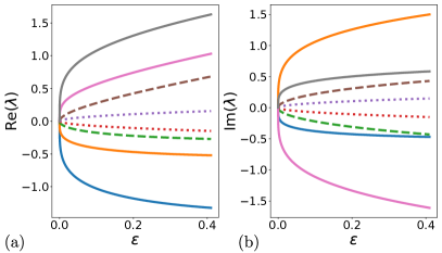
Figure 4: Real (a) and imaginary (b) parts of the eigenvalues $\lambda$ of the matrix $M_{3}$, governing third-order FMs, at the EP $g=\Delta$, under the perturbation $\epsilon$, which enables resolving a DDEP. The matrix $M_{3}$ has a single EP of fourth order (presented by the coalescence of four solid curves, characterized by the quartic-root dependence on perturbation, $\sqrt[4]{\epsilon}$). Apart from it, under the perturbation, the initial DDEP splits into two EPs of second order (presented by the merge of two eigenvalues, shown by the two dashed and two dotted curves, respectively, which are characterized by the square-root dependence of the perturbation, $\sqrt{\epsilon}$).

The corresponding eigenvectors are easily found, according to Eq. (6),

$$\psi^{(3)}=\left(\begin{array}[]{cccccccc}-{{\rm e}^{-3\,i\phi}}&{{\rm e}^{-i\phi}}&{{\rm e}^{-i\phi}}&-{{\rm e}^{i\phi}}&{{\rm e}^{-i\phi}}&-{{\rm e}^{i\phi}}&-{{\rm e}^{i\phi}}&{{\rm e}^{3\,i\phi}}\\ \vskip 6.0pt plus 2.0pt minus 2.0pt\cr{{\rm e}^{-2\,i\phi}}&{{\rm e}^{-2\,i\phi}}&-1&-1&-1&-1&{{\rm e}^{2\,i\phi}}&{{\rm e}^{2\,i\phi}}\\ \vskip 6.0pt plus 2.0pt minus 2.0pt\cr{{\rm e}^{-2\,i\phi}}&-1&{{\rm e}^{-2\,i\phi}}&-1&-1&{{\rm e}^{2\,i\phi}}&-1&{{\rm e}^{2\,i\phi}}\\ \vskip 6.0pt plus 2.0pt minus 2.0pt\cr-{{\rm e}^{-i\phi}}&-{{\rm e}^{-i\phi}}&-{{\rm e}^{-i\phi}}&-{{\rm e}^{-i\phi}}&{{\rm e}^{i\phi}}&{{\rm e}^{i\phi}}&{{\rm e}^{i\phi}}&{{\rm e}^{i\phi}}\\ \vskip 6.0pt plus 2.0pt minus 2.0pt\cr{{\rm e}^{-2\,i\phi}}&-1&-1&{{\rm e}^{2\,i\phi}}&{{\rm e}^{-2\,i\phi}}&-1&-1&{{\rm e}^{2\,i\phi}}\\ \vskip 6.0pt plus 2.0pt minus 2.0pt\cr-{{\rm e}^{-i\phi}}&-{{\rm e}^{-i\phi}}&{{\rm e}^{i\phi}}&{{\rm e}^{i\phi}}&-{{\rm e}^{-i\phi}}&-{{\rm e}^{-i\phi}}&{{\rm e}^{i\phi}}&{{\rm e}^{i\phi}}\\ \vskip 6.0pt plus 2.0pt minus 2.0pt\cr-{{\rm e}^{-i\phi}}&{{\rm e}^{i\phi}}&-{{\rm e}^{-i\phi}}&{{\rm e}^{i\phi}}&-{{\rm e}^{-i\phi}}&{{\rm e}^{i\phi}}&-{{\rm e}^{-i\phi}}&{{\rm e}^{i\phi}}\\ \vskip 6.0pt plus 2.0pt minus 2.0pt\cr 1&1&1&1&1&1&1&1\end{array}\right).$$ (45)

Note that the two eigenvalues $\pm\Lambda$ are triply degenerate. At the EP $g=\Delta$, the Jordan form of $M_{3}$ reads

$$M_{3}^{\rm EP}=\left(\begin{array}[]{cccccccc}0&1&0&0&0&0&0&0\\ \vskip 6.0pt plus 2.0pt minus 2.0pt\cr 0&0&1&0&0&0&0&0\\ \vskip 6.0pt plus 2.0pt minus 2.0pt\cr 0&0&0&1&0&0&0&0\\ \vskip 6.0pt plus 2.0pt minus 2.0pt\cr 0&0&0&0&0&0&0&0\\ \vskip 6.0pt plus 2.0pt minus 2.0pt\cr 0&0&0&0&0&1&0&0\\ \vskip 6.0pt plus 2.0pt minus 2.0pt\cr 0&0&0&0&0&0&0&0\\ \vskip 6.0pt plus 2.0pt minus 2.0pt\cr 0&0&0&0&0&0&0&1\\ \vskip 6.0pt plus 2.0pt minus 2.0pt\cr 0&0&0&0&0&0&0&0\end{array}\right),$$ (54)

The effective dimension of $M_{3}$ is four [$S_{3}(2)=4$], and, therefore, there is a single EP of fourth order. However, apart from this EP, also one DDEP of second order emerges, due to the triply degenerated pairs of eigenvalues.

In order to lift the degeneracy of the DDEP, one can induce a specific perturbation to the matrix $M_{3}$, i.e., $M_{3}\to M_{3}+\epsilon P$, where $\epsilon$ denotes the perturbation strength. The matrix $P$ can read:

$$P={\rm diag}\left[1,0,0,1,0,1,0,0\right].$$ (55)

The result of such a perturbation on the eigenvalues of $M_{3}$ is shown in Fig. 4. Other choices of perturbation do not necessarily lead to the DDEP detection. Note that the perturbation is actually fictitious because of the symmetry protection of the evolution matrix $M_{3}$ in the FM space. Indeed, by unfolding the evolution matrices $M_{3}$ from the first-order moments $2\times 2$ matrix $M_{1}$, it is impossible to attain such a perturbed matrix $M_{3}$. However, the formation of such DDEP in the spectrum can be checked by mapping the evolution matrix $M_{3}$ to a certain real-space photonic-lattice Hamiltonian.

Importantly, the above revealed hybrid spectral features of FMs polytopes can also be exploited in the construction of similar non-Hermitian Hamiltonians in real space. For instance, one of the nontrivial outcomes of the presence of a DDEP in the spectrum of real multimode non-Hermitian Hamiltonians can be the implementation of a programmable multimode switch by dynamically encircling the DDEP [55]. A direct detection of DDEPs in the FMs space of a bosonic system can be performed by measuring bosonic commutators [71] and/or anomalous FMs [72]. The tensor-product-states structure of a FM space can also be recovered from Cahill-Glauber $s$-ordered FMs, which can be obtained from the measured normally-ordered moments using standard photon-detection schemes [68, 73, 74]. Note that our conclusions remain valid also for the quadrature field moments, which could be easier to access experimentally, e.g., via standard balanced homodyne detection [65, 75].

Appendix D Triangular and Tetrahedral non-Hermitian lattice models in the field-moments space of three- and four-mode systems, respectively

D.1 Triangular non-Hermitian lattice model with open boundaries

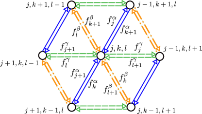
Figure 5: An element of the triangle-shaped triangular non-Hermitian lattice model in Fig. 3(c), described by the non-Hermitian Hamiltonian in Eq. (57), illustrating the nearest-neighbor interactions for a site with indices $(j,k,l)$ (shown in the centre). The site potentials and couplings $f^{\xi}_{q}$ are given in Eqs. (58) and (59), respectively.

We have already mentioned about the emergence of a triangular lattice in the FMs space of a three-mode system, as depicted in Fig. 3. Here we discuss in a more detail the structure of such a lattice, its mapping to a non-Hermitian Hamiltonian, and shortly mention the tetrahedral lattices appearing in the FMs space of four-mode systems.

For the sake of clarity, we repeat some parts of the main text. First, let us consider the first-order FMs vector $\langle\hat{\Phi}\rangle$ of a three-mode system, where $\hat{\Phi}=[\hat{a}_{1},\hat{a}_{2},\hat{a}_{3}]^{T}$, which is governed by the following symmetric evolution matrix:

$$M_{1}=\begin{pmatrix}\Delta_{1}&\alpha&\gamma\\ \alpha&\Delta_{2}&\beta\\ \gamma&\beta&\Delta_{3}\end{pmatrix}.$$ (56)

Compared to the Eq. (10), we also add the diagonal terms $\Delta_{k}$, which can be associated with different resonant (complex) frequencies of the interacting modes. The degenerate evolution matrix $M_{N}$ governing the dynamics of the $N$th-order FM ${\langle\bigotimes^{N}_{1}\hat{\Phi}\rangle}$ is obtained from $M_{1}$ according to Eq. (4). The matrix $M_{N}$ then describes a highly degenerate $2N$-polytope [the case for $N=1,2$ is shown in Fig. 1(b)]. This extra degeneracy can be eliminated by effectively reducing the $2N$-polytope with $3^{N}$ vertices to a two-dimensional triangular ISCs having $S_{N}(3)$ vertices instead (see also Fig. 3). This folding procedure is accompanied by the reduction of the symmetric evolution matrix $M_{N}$ to the asymmetric effective matrix $M_{N}^{\rm eff}$.

One then can relate the effective evolution matrix $M^{\rm eff}_{N}$ to a non-Hermitian Hamiltonian describing a triangle-shaped triangular lattice (shown in Fig. 3). One can see that the hopping amplitudes have the maximal values for the sites on the boundary, being proportional to the size of the corresponding external or internal triangle lattice edges. The tunneling amplitudes are steadily decreasing when approaching the opposite sides of the triangular lattice, revealing the characteristic asymmetry in the site interactions, i.e., their path dependence. The eigendecomposition of the non-Hermitian Hamiltonian $\hat{H}^{N}$, which is identical to the matrix $M^{\rm eff}_{N}$, directly follows from the eigendecomposition of the matrix $M_{N}$, as was discussed in the previous section. Since the spectrum of $M_{N}$ can be readily calculated, so the eigenspectrum of the non-Hermitian Hamiltonian $\hat{H}^{N}$.

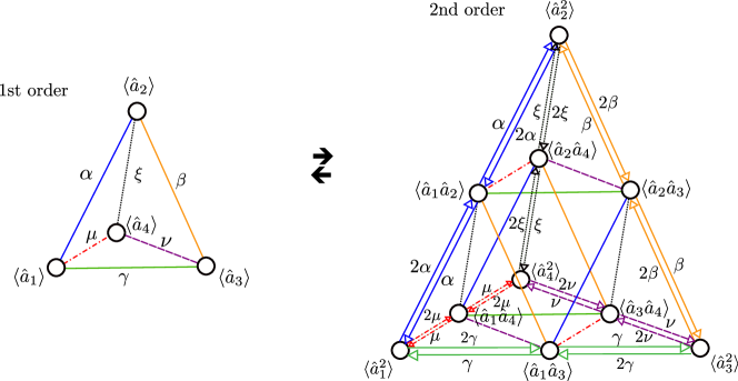
Figure 6: Formation of iterated simplex chains by folding iterated polytope chains in the field-moments space of bosonic four-mode systems. (a) A 3-simplex, i.e., a tetrahedron, formed in the first-order FMs, which coincides with the $P_{i_{1}}$ polytope. The links, denoted by Greek letters $\alpha,\beta,\gamma,\mu,\xi,\nu$, and highlighted by different colors, correspond to the coupling strengths between the three FMs. (b) An ISC in the second-order FMs space. By folding the corresponding symmetric $6$-polytope, one obtains an asymmetric $3$-simplex, namely a tetrahedral-octahedral honeycomb in the high-order FMs space of the four-mode bosonic system.

Namely, by inducing the map $M^{\rm eff}_{N}\to\hat{H}^{N}$, one attains:

$$\hat{H}^{N}=\hat{H}_{0}^{N}+\hat{H}_{\rm int}^{N},$$ (57)

where $\hat{H}_{0}^{N}$ accounts for the non-interacting Hamiltonian part describing ‘site potentials’ on the triangular lattice, which reads

$$\hat{H}^{N}_{0}=\sum\limits_{\begin{subarray}{c}j,k=1\\ l=N-j-k\end{subarray}}^{N}\left(j\Delta_{1}+k\Delta_{2}+l\Delta_{3}\right)\hat{c}^{\dagger}_{j,k,l}\hat{c}_{j,k,l},$$ (58)

and asymmetric ‘site interactions’ are described by the part:

$$\hat{H}^{N}_{\rm int}= \sum\limits_{\begin{subarray}{c}j,k=1\\ l=N-j-k\end{subarray}}^{N}\hat{c}_{j,k,l}\Big{(}f_{j}^{\alpha}\hat{c}^{\dagger}_{j-1,k+1,l}+f_{j}^{\gamma}\hat{c}^{\dagger}_{j-1,k,l+1}$$ (59)

$$+f_{k}^{\beta}\hat{c}^{\dagger}_{j,k-1,l+1}+f_{k}^{\alpha}\hat{c}^{\dagger}_{j+1,k-1,l}$$

$$+f_{l}^{\gamma}\hat{c}^{\dagger}_{j+1,k,l-1}+f_{l}^{\beta}\hat{c}^{\dagger}_{j,k+1,l-1}\Big{)}$$

$$+\hat{c}^{\dagger}_{j,k,l}\Big{(}f_{k+1}^{\alpha}\hat{c}_{j-1,k+1,l}+f_{l+1}^{\gamma}\hat{c}_{j-1,k,l+1}$$

$$+f_{l+1}^{\beta}\hat{c}_{j,k-1,l+1}+f_{j+1}^{\alpha}\hat{c}_{j+1,k-1,l}$$

$$+f_{j+1}^{\gamma}\hat{c}_{j+1,k,l-1}+f_{k+1}^{\beta}\hat{c}_{j,k+1,l-1}\Big{)},$$

where the hopping coefficients read $f^{\xi}_{q}=q\xi$. An element of such a lattice is also shown in Fig. 5.

D.2 Tetrahedral non-Hermitian lattice model with open boundaries

In a similar fashion, one can obtain a $3$-simplex non-Hermitian lattice, namely a non-Hermitian tetrahedral-octahedral honeycomb model, emerging in the ISCc FMs space of a four-mode system, whose first-order FMs symmetric evolution matrix has the following generic form

$$M_{1}=\begin{pmatrix}\Delta_{1}&\alpha&\gamma&\mu\\ \alpha&\Delta_{2}&\beta&\xi\\ \gamma&\beta&\Delta_{3}&\nu\\ \mu&\xi&\nu&\Delta_{4}\end{pmatrix}.$$ (60)

The schematic representation of the 3-simplex described by the matrix $M_{1}$ is shown in Fig. 6(a). The second-order FMs evolution matrix $M_{2}$ is then an augmented tetrahedron from below [see Fig. 6(b)]. Similarly, one obtains an iterated 3-simplex chain comprised by tetrahedrons for arbitrary high-order FMs.

Appendix E Symmetrization of non-Hermitian $n$-simplex lattices

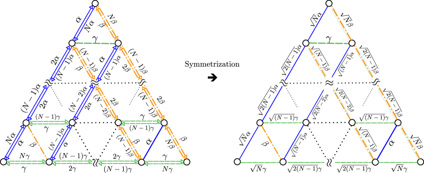
Figure 7: Symmetrization of the asymmetric 2-simplex lattice (left panel), also shown in Fig. 3(c), to the symmetric 2-simplex lattice (right panel). In other words, the asymmetric intersite couplings (depicted as double arrows on the left panel) become symmetric (shown by single arrows on the right panel). This mapping can realized via an appropriate similarity transformation, or, alternatively, by choosing an appropriate basis when projecting polytopes onto simplexes, formed in the field-moments space of quadratic systems. The edges of the symmetric 2-simplex lattice can describe a quantum angular momentum operator with different quantum numbers. See more details in Appendix E.

As was mentioned in Sec. II.5 and Sec. III of the main text, the asymmetric $n$-simplex lattices, emerging in the FMS of quadratic systems, can be transformed into symmetric ones by finding an appropriate similarity transformation, or, in other words, by choosing an appropriate basis when performing a projection of IPCs onto ISCs. This means that because of such lattice symmetrization only eigenvectors are modified, whereas eigenvalues are left the same.

In the third bullet of Appendix B, we have pointed that a general $(2N)^{m}\times S_{m}(2N)$ matrix $B^{\prime}$, which defines the basis of the polytopes projection on their non-degenerate space is composed of $S_{m}$ column-vectors, where $S_{m}$ is given in Eq. (8). Some of these column-vectors are formed as a symmetrical combination, i.e., an average, of column-vectors of the identity matrix $I_{(2N)^{m}}$. However, if instead of that ‘average’ of $D_{i}$ basis vectors, factored by $1/D_{i}$ (see Eq. (20)), to take the same combination but factored by $1\sqrt{D_{i}}$, i.e., a normalized sum, then the new resulting transformation matrix $T=B^{\prime T}A^{\prime}$ would produce a symmetric effective matrix $M_{m}^{\rm eff}$, which describes the symmetrized $n$-simplex lattice.

Let us explain this in more detail by considering a simple example, similar to that in Appendix C.2. That is, we would like to symmetrize the matrix $M^{\rm eff}_{2}$ in Eq. (33). For that, instead of the matrix $B^{\prime}$, in Eq. (30), we take a new matrix $B^{\prime\prime}$, now formed by normalized column-vectors, i.e.,

$$B^{\prime}\to B^{\prime\prime}=\begin{pmatrix}1&0&0\\ 0&\dfrac{1}{\sqrt{2}}&0\\ 0&\dfrac{1}{\sqrt{2}}&0\\ 0&0&1\end{pmatrix}.$$ (61)

By constructing a modified transformation matrix $T^{\prime}=B^{\prime\prime T}A^{\prime}$, where $A^{\prime}$ is the same as in Eq. (29), one obtains the symmetrical matrix $M_{2,\rm sym}^{\rm eff}$ in the form

$$M_{2,\rm sym}^{\rm eff}=T^{\prime}DT^{\prime-1}=\begin{pmatrix}-2i\Delta&-\sqrt{2}g&0\\ -\sqrt{2}g&0&-\sqrt{2}g\\ 0&-\sqrt{2}g&2i\Delta\end{pmatrix},$$

where diagonal matrix $D$ is given in Eq. (31). For a two-mode system, one can then show that an arbitrary $M_{m}^{\rm eff}$ matrix is similar to the symmetric matrix $M_{m,\rm sym}^{\rm eff}$ via the transformation in Eq. (13).

One can straightforwardly verify that this symmetrization procedure is extended to any effective matrix $M_{m}^{\rm eff}$ describing an $n$-simplex lattice. For instance, for a 2-simplex lattice, with asymmetrical bidirectional links as shown in Fig. 3(c), the described symmetrization procedure allows to transform that lattice into symmetrical one, where the intersite couplings become symmetric (see Fig. 7).

Remarkably, due to this symmetrization of $M_{m}^{\rm eff}$, the resulting symmetric $n$-simplex lattices have 1D edges which can be mapped to the angular momentum operator $\hat{J}_{z}$ in the Fock space representation (up to a certain scaling factor, proportional to a bosonic mode coupling), provided that the diagonal elements of $M_{m}^{\rm eff}$ are zero. Indeed, according to Fig. 7, all (anti-) diagonal and horizontal edges of the symmetric 2-simplex lattice can represent the angular momentum operator with a certain azimuthal quantum number $j$, which is determined by the number of vertices belonging to the corresponding edge.

For instance, the submatrices of $M_{m}^{\rm eff}$ describing three outer edges in Fig. 7, which contain $(N+1)$ vertices, correspond to the angular momentum operator with the quantum number $j=N/2$ (see also Sec. III), with additional scaling factors $\alpha$, $\beta$, and $\gamma$ (see Fig. 7). In general, an edge having $K$ vertices is related to the angular momentum quantum number $j=(K-1)/2$ (see Fig. 7).

References

- Aizenman and Lieb [1981] M. Aizenman and E. Lieb, The third law of thermodynamics and the degeneracy of the ground state for lattice systems, J. Stat. Phys. 24, 279 (1981).
- Wu et al. [2013] X. Wu, N. Izmailian, and W. Guo, Shape-dependent finite-size effect of the critical two-dimensional Ising model on a triangular lattice, Phys. Rev. E 87, 022124 (2013).
- Baxter [2020] R. J. Baxter, The bulk, surface and corner free energies of the anisotropic triangular Ising model, Proc. R. Soc. A. 476, 20190713 (2020).
- Hatano and Nelson [1996] N. Hatano and D. R. Nelson, Localization transitions in non-Hermitian quantum mechanics, Phys. Rev. Lett. 77, 570 (1996).
- Ashida et al. [2020] Y. Ashida, Z. Gong, and M. Ueda, Non-Hermitian physics, Adv. Phys. 69, 249–435 (2020).
- Bergholtz et al. [2021] E. J. Bergholtz, J. C. Budich, and F. K. Kunst, Exceptional topology of non-Hermitian systems, Rev. Mod. Phys. 93, 015005 (2021).
- Ding et al. [2022] K. Ding, C. Fang, and G. Ma, Non-Hermitian topology and exceptional-point geometries, Nat. Rev. Phys. 4, 745 (2022).
- Scheffé [1958] H. Scheffé, Experiments with mixtures, J. Roy. Stat. Soc. B 20, 344 (1958).
- Luther and Squire [1980] P. K. Luther and J. M. Squire, Three-dimensional structure of the vertebrate muscle A-band: Ii. The myosin filament superlattice, J. Mol. Biol. 141, 409 (1980).
- Grünbaum [2003] B. Grünbaum, Convex polytopes (Springer; 2nd edition, New York & London, 2003).
- Nelson and Widom [1984] D. R. Nelson and M. Widom, Symmetry, Landau theory and polytope models of glass, Nucl. Phys. B 240, 113 (1984).
- Baxter [1985] R. J. Baxter, Exactly solved models in statistical mechanics, in Integrable Systems in Statistical Mechanics (1985) pp. 5–63.
- Kundu [2003] A. Kundu, ed., Classical and Quantum Nonlinear Integrable Systems: Theory and Application (CRC Press, 2003).
- Kitaev [2006] A. Kitaev, Anyons in an exactly solved model and beyond, Ann. Phys. 321, 2 (2006).
- Yao and Kivelson [2007] H. Yao and S. A. Kivelson, Exact chiral spin liquid with non-Abelian anyons, Phys. Rev. Lett. 99, 247203 (2007).
- Nussinov and Ortiz [2009] Z. Nussinov and G. Ortiz, Bond algebras and exact solvability of Hamiltonians: Spin multilayer systems, Phys. Rev. B 79, 214440 (2009).
- Leumer et al. [2020] N. Leumer, M. Marganska, B. Muralidharan, and M. Grifoni, Exact eigenvectors and eigenvalues of the finite Kitaev chain and its topological properties, J. Phys.: Condens. Matter. 32, 445502 (2020).
- Orús [2019] R. Orús, Tensor networks for complex quantum systems, Nat. Rev. Phys. 1, 538 (2019).
- Carleo et al. [2019] G. Carleo et al., Machine learning and the physical sciences, Rev. Mod. Phys. 91 (2019).
- Kalugin et al. [1985] P. A. Kalugin, A. Y. Kitaev, and L. S. Levitov, : a six-dimensional crystal, Pis’ma Zh. Eksp. Teor. Phys. 41, 119 (1985).
- Elser [1985] V. Elser, Indexing problems in quasicrystal diffraction, Phys. Rev. B 32, 4892 (1985).
- Katz and Duneau [1986] A. Katz and M. Duneau, Quasiperiodic patterns and icosahedral symmetry, J. Phys. France 47, 181 (1986).
- Nori et al. [1988] F. Nori, M. Ronchetti, and V. Elser, Strain accumulation in quasicrystalline solids, Phys. Rev. Lett. 61, 2774 (1988).
- Baake et al. [1991] M. Baake, D. Joseph, and P. Kramer, The Schur rotation as a simple approach to the transition between quasiperiodic and periodic phases, J. Phys. A: Math. Gen. 24, L961 (1991).
- Narducci and Orszag [1972] L. M. Narducci and M. Orszag, Eigenvalues and Eigenvectors of Angular Momentum Operator without the Theory of Rotations, Am. J. Phys. 40, 1811 (1972).
- Hu [2021] Z. Hu, Eigenvalues and eigenvectors of a class of irreducible tridiagonal matrices, Lin. Alg. Appl. 619, 328 (2021).
- Joglekar and Saxena [2011] Y. N. Joglekar and A. Saxena, Robust -symmetric chain and properties of its Hermitian counterpart, Phys. Rev. A 83, 050101 (2011).
- Arkhipov and Minganti [2023] I. I. Arkhipov and F. Minganti, Emergent non-Hermitian localization phenomena in the synthetic space of zero-dimensional bosonic systems, Phys. Rev. A 107, 012202 (2023).
- Daley et al. [2022] A. J. Daley, I. Bloch, C. Kokail, et al., Practical quantum advantage in quantum simulation, Nature (London) 607, 667 (2022).
- Nori and Lin [1994] F. Nori and Y.-L. Lin, Analytical solution for the Fermi-sea energy of two-dimensional electrons in a magnetic field: Lattice path-integral approach and quantum interference, Phys. Rev. B 49, 4131 (1994).
- Lin and Nori [1996a] Y.-L. Lin and F. Nori, Quantum interference from sums over closed paths for electrons on a three-dimensional lattice in a magnetic field: Total energy, magnetic moment, and orbital susceptibility, Phys. Rev. B 53, 13374 (1996a).
- Lin and Nori [1996b] Y.-L. Lin and F. Nori, Strongly localized electrons in a magnetic field: Exact results on quantum interference and magnetoconductance, Phys. Rev. Lett. 76, 4580 (1996b).
- Lin and Nori [1996c] Y.-L. Lin and F. Nori, Analytical results on quantum interference and magnetoconductance for strongly localized electrons in a magnetic field: Exact summation of forward-scattering paths, Phys. Rev. B 53, 15543 (1996c).
- Lin and Nori [2002] Y.-L. Lin and F. Nori, Quantum interference in superconducting wire networks and Josephson junction arrays: An analytical approach based on multiple-loop Aharonov-Bohm Feynman path integrals, Phys. Rev. B 65, 214504 (2002).
- Regensburger et al. [2012] A. Regensburger, C. Bersch, M.-A. Miri, G. Onishchukov, D. N. Christodoulides, and U. Peschel, Parity-time synthetic photonic lattices, Nature (London) 488, 167 (2012).
- Yuan et al. [2018] L. Yuan, Q. Lin, M. Xiao, and S. Fan, Synthetic dimension in photonics, Optica 5, 1396 (2018).
- Ozawa and Price [2019] T. Ozawa and H. M. Price, Topological quantum matter in synthetic dimensions, Nat. Rev. Phys. 1, 349 (2019).
- Lustig et al. [2019] E. Lustig, S. Weimann, Y. Plotnik, Y. Lumer, M. A. Bandres, A. Szameit, and M. Segev, Photonic topological insulator in synthetic dimensions, Nature (London) 567, 356–360 (2019).
- Fabre et al. [2022] A. Fabre, J.-B. Bouhiron, T. Satoor, R. Lopes, and S. Nascimbene, Simulating two-dimensional dynamics within a large-size atomic spin, Phys. Rev. A 105, 013301 (2022).
- Weimann et al. [2017] S. Weimann, M. Kremer, Y. Plotnik, Y. Lumer, S. Nolte, K. Makris, M. Segev, M. Rechtsman, and A. Szameit, Topologically protected bound states in photonic parity–time-symmetric crystals, Nat. Mater. 16, 433 (2017).
- Roy et al. [2021a] A. Roy, M. Parto, R. Nehra, C. Leefmans, and A. Marandi, Topological optical parametric oscillation (2021a), arXiv:2108.01287 .
- Weidemann et al. [2020] S. Weidemann, M. Kremer, T. Helbig, T. Hofmann, A. Stegmaier, M. Greiter, R. Thomale, and A. Szameit, Topological funneling of light, Science 368, 311 (2020).
- Teimourpour et al. [2014] M. H. Teimourpour, R. El-Ganainy, A. Eisfeld, A. Szameit, and D. N. Christodoulides, Light transport in -invariant photonic structures with hidden symmetries, Phys. Rev. A 90, 053817 (2014).
- Quiroz-Juárez et al. [2019] M. A. Quiroz-Juárez, A. Perez-Leija, K. Tschernig, B. M. Rodríguez-Lara, O. S. Magaña-Loaiza, K. Busch, Y. N. Joglekar, and R. J. León-Montiel, Exceptional points of any order in a single, lossy waveguide beam splitter by photon-number-resolved detection, Photon. Res. 7, 862 (2019).
- Tschernig et al. [2020] K. Tschernig, R. J. León-Montiel, A. Pérez-Leija, and K. Busch, Multiphoton synthetic lattices in multiport waveguide arrays: synthetic atoms and Fock graphs, Photon. Res. 8, 1161 (2020).
- Kok et al. [2007] P. Kok, W. J. Munro, K. Nemoto, T. C. Ralph, J. P. Dowling, and G. J. Milburn, Linear optical quantum computing with photonic qubits, Rev. Mod. Phys. 79, 135 (2007).
- Arkhipov et al. [2021] I. I. Arkhipov, F. Minganti, A. Miranowicz, and F. Nori, Generating high-order quantum exceptional points in synthetic dimensions, Phys. Rev. A 104, 012205 (2021).
- Candan et al. [2000] C. Candan, M. Kutay, and H. Ozaktas, The discrete fractional Fourier transform, IEEE Trans. Signal Process. 48, 1329 (2000).
- Weimann et al. [2016] S. Weimann, A. Perez-Leija, M. Lebugle, et al., Implementation of quantum and classical discrete fractional Fourier transforms, Nat. Commun. 7, 11027 (2016).
- Zhou et al. [2017] Y. Zhou, M. Mirhosseini, D. Fu, J. Zhao, S. M. Hashemi R., A. E. Willner, and R. W. Boyd, Sorting photons by radial quantum number, Phys. Rev. Lett. 119, 263602 (2017).
- Niewelt et al. [2023] B. Niewelt, M. Jastrzębski, S. Kurzyna, J. Nowosielski, W. Wasilewski, M. Mazelanik, and M. Parniak, Experimental implementation of the optical fractional Fourier transform in the time-frequency domain, Phys. Rev. Lett. 130, 240801 (2023).
- Lototsky [2015] S. Lototsky, Simple spectral bounds for sums of certain Kronecker products, Lin. Alg. Appl. 469, 114 (2015).
- Perina Jr. et al. [2022] J. Perina Jr., A. Miranowicz, G. Chimczak, and A. Kowalewska-Kudlaszyk, Quantum Liouvillian exceptional and diabolical points for bosonic fields with quadratic Hamiltonians: The Heisenberg-Langevin equation approach, Quantum 6, 883 (2022).
- Ş. K. Özdemir et al. [2019] Ş. K. Özdemir, S. Rotter, F. Nori, and L. Yang, Parity-time symmetry and exceptional points in photonics, Nat. Mater. 18, 783 (2019).
- Arkhipov et al. [2023] I. I. Arkhipov, A. Miranowicz, F. Minganti, Ş. K. Özdemir, and F. Nori, Dynamically crossing diabolic points while encircling exceptional curves: A programmable symmetric-asymmetric multimode switch, Nat. Commun. 14, 2076 (2023).
- Kato [1995] T. Kato, Perturbation theory for linear operators, Classics in Mathematics (Springer, Berlin, 1995).
- Doria et al. [2011] P. Doria, T. Calarco, and S. Montangero, Optimal control technique for many-body quantum dynamics, Phys. Rev. Lett. 106, 190501 (2011).
- Khaneja et al. [2005] N. Khaneja, T. Reiss, C. Kehlet, T. Schulte-Herbrüggen, and S. J. Glaser, Optimal control of coupled spin dynamics: design of NMR pulse sequences by gradient ascent algorithms, J. Magn. Reson. 172, 296 (2005).
- Sakurai and Napolitano [2020] J. J. Sakurai and J. Napolitano, Modern Quantum Mechanics (Cambridge University Press, Cambridge, 2020).
- Asano et al. [2019] M. Asano, R. Ohta, T. Aihara, T. Tsuchizawa, H. Okamoto, and H. Yamguchi, Optically probing Schwinger angular momenta in a micromechanical resonator, Phys. Rev. A 100, 053801 (2019).
- Heiss and Sannino [1991] W. D. Heiss and A. L. Sannino, Transitional regions of finite Fermi systems and quantum chaos, Phys. Rev. A 43, 4159 (1991).
- Wick [1950] G. C. Wick, The evaluation of the collision matrix, Phys. Rev. 80, 268 (1950).
- Jagannathan [2021] A. Jagannathan, The Fibonacci quasicrystal: Case study of hidden dimensions and multifractality, Rev. Mod. Phys. 93, 045001 (2021).
- Falconer [2014] K. Falconer, Fractal Geometry: Mathematical Foundations and Applications (John Wiley & Sons, UK, 2014).
- Wang and Clerk [2019] Y.-X. Wang and A. A. Clerk, Non-Hermitian dynamics without dissipation in quantum systems, Phys. Rev. A 99, 063834 (2019).
- Roy et al. [2021b] A. Roy, S. Jahani, Q. Guo, A. Dutt, S. Fan, M.-A. Miri, and A. Marandi, Nondissipative non-Hermitian dynamics and exceptional points in coupled optical parametric oscillators, Optica 8, 415 (2021b).
- Flynn et al. [2020] V. P. Flynn, E. Cobanera, and L. Viola, Deconstructing effective non-Hermitian dynamics in quadratic bosonic Hamiltonians, New J. Phys. 22, 083004 (2020).
- Peřina [1991] J. Peřina, Quantum Statistics of Linear and Nonlinear Optical Phenomena (Kluwer, Dordrecht, 1991).
- Christodoulides and Yang [2018] D. Christodoulides and J. Yang, eds., Parity-time Symmetry and Its Applications (Springer Singapore, 2018).
- El-Ganainy et al. [2018] R. El-Ganainy, K. G. Makris, M. Khajavikhan, Z. H. Musslimani, S. Rotter, and D. N. Christodoulides, Non-Hermitian physics and symmetry, Nat. Phys. 14, 11 (2018).
- Zavatta et al. [2009] A. Zavatta, V. Parigi, M. S. Kim, H. Jeong, and M. Bellini, Experimental demonstration of the bosonic commutation relation via superpositions of quantum operations on thermal light fields, Phys. Rev. Lett. 103, 140406 (2009).
- Kühn et al. [2017] B. Kühn, W. Vogel, M. Mraz, S. Köhnke, and B. Hage, Anomalous quantum correlations of squeezed light, Phys. Rev. Lett. 118, 153601 (2017).
- Peřina et al. [2017] J. Peřina, I. I. Arkhipov, V. Michálek, and O. Haderka, Nonclassicality and entanglement criteria for bipartite optical fields characterized by quadratic detectors, Phys. Rev. A 96, 043845 (2017).
- Shchukin and Vogel [2005] E. V. Shchukin and W. Vogel, Nonclassical moments and their measurement, Phys. Rev. A 72, 043808 (2005).
- Roccati et al. [2021] F. Roccati, S. Lorenzo, G. M. Palma, G. T. Landi, M. Brunelli, and F. Ciccarello, Quantum correlations in -symmetric systems, Quantum Sci. Technol. 6, 025005 (2021).