Optimization-Induced Graph Implicit Nonlinear Diffusion

Abstract

Due to the over-smoothing issue, most existing graph neural networks can only capture limited dependencies with their inherently finite aggregation layers. To overcome this limitation, we propose a new kind of graph convolution, called Graph Implicit Nonlinear Diffusion (GIND), which implicitly has access to infinite hops of neighbors while adaptively aggregating features with nonlinear diffusion to prevent over-smoothing. Notably, we show that the learned representation can be formalized as the minimizer of an explicit convex optimization objective. With this property, we can theoretically characterize the equilibrium of our GIND from an optimization perspective. More interestingly, we can induce new structural variants by modifying the corresponding optimization objective. To be specific, we can embed prior properties to the equilibrium, as well as introducing skip connections to promote training stability. Extensive experiments show that GIND is good at capturing long-range dependencies, and performs well on both homophilic and heterophilic graphs with nonlinear diffusion. Moreover, we show that the optimization-induced variants of our models can boost the performance and improve training stability and efficiency as well. As a result, our GIND obtains significant improvements on both node-level and graph-level tasks.

1 Introduction

In recent years, graph neural networks (GNNs) rise to be the state-of-the-art models for graph mining (Kipf & Welling, 2016; Veličković et al., 2017; Hamilton et al., 2017; Li et al., 2022a) and have extended applications in various scenarios such as biochemical structure discovery (Gilmer et al., 2017; Wan et al., 2019), recommender systems (Ying et al., 2018; Fan et al., 2019), natural language processing (Gao et al., 2019; Zhu et al., 2019), and computer vision (Pang & Cheung, 2017; Valsesia et al., 2020). Despite the success, these GNNs typically lack the ability to capture long-range dependencies. In particular, the common message-passing GNNs can only aggregate information from $T$-hop neighbors with $T$ propagation steps. However, existing works have observed that GNNs often degrade catastrophically when propagation steps $T\geq 2$ (Li et al., 2018), a phenomenon widely characterized as over-smoothing. Several works try to alleviate it with more expressive aggregations of higher-order neighbors (Abu-El-Haija et al., 2019; Zhu et al., 2020). Nevertheless, their ability to capture global information is inherently limited by the finite propagation steps.

Recently, implicit GNNs provide a new solution to this problem by replacing the deeply stacked explicit propagation layers with an implicit layer, which is equivalent to infinite propagation steps (Gu et al., 2020; Liu et al., 2021a; Park et al., 2021). Thereby, implicit GNNs could capture very long range dependencies and benefit from the global receptive field. Specifically, implicit GNNs achieve this by regularizing the explicit forward propagation to a root-finding problem with convergent equilibrium states. They further adopt implicit differentiation (Krantz & Parks, 2012) directly through the equilibrium states to avoid long range back-propagation. As a result, the methods could get rid of performance degradation caused by explosive variance with more depth (Zhou et al., 2021) while having constant memory footprint even with infinite propagation steps. These advantages indicate that implicit GNNs are promising alternatives to existing explicit GNNs.

The performance of implicit GNNs is largely determined by the design of the implicit layer. However, it is overlooked by previous works. Their implicit layers are direct adaptations of recurrent GNNs (Gu et al., 2020) and lack theoretical justifications of their diffusion properties. Notably, a major drawback is that their aggregation mechanisms correspond to a linear isotropic diffusion that treats all neighbors equally. However, as noted by recent theoretical discussions (Oono & Suzuki, 2019), this isotropic property is exactly the cause of the over-smoothing issue. Thus, it is still hard for them to benefit from long range dependencies. This problem reveals that the infinite depth itself is inadequate. The design of the diffusion process, which decides the quality of the equilibrium states, is also the key to the actual performance of implicit GNNs.

Motivated by this situation, in this work, we propose a novel and principled implicit graph diffusion layer, whose advantages are two folds. First, drawing inspirations from anisotropic diffusion process like PM diffusion (Perona & Malik, 1990), we extend the linear isotropic diffusion to a more expressive nonlinear diffusion mechanism, which learns nonlinear flux features between node pairs before aggregation. In particular, our design of the nonlinear diffusion ensures that more information can be aggregated from similar neighbors and less from dissimilar neighbors, making node features less likely to over-smooth. Second, we can show for the first time that the equilibrium of our implicit nonlinear diffusion is the solution to a convex optimization objective. Based on this perspective, we can not only characterize theoretical properties of the equilibrium states, but also derive new structural variants in a principled way, e.g., adding regularization terms to the convex objective.

Based on the above analysis, we propose a model named Graph Implicit Nonlinear Diffusion (GIND). Several recent works have tried to connect GNN propagations to structural optimization objectives (Zhu et al., 2021; Yang et al., 2021; Ma et al., 2021; Liu et al., 2021b). However, their frameworks only consider aggregation steps and ignore the nonlinear transformation of features, which is also crucial in GNNs. In comparison, our GIND admits a unified objective of both the nonlinear diffusion step and the transformation step. Therefore, our framework is more general, as it could take the interaction between diffusion and transformation into consideration. Last but not least, compared to previous optimization-based GNNs whose propagation rule is inspired by one single optimization step, our GIND directly models the equilibrium of the implicit layer as a minimizer of a convex objective (thus we call it optimization-induced). This shows that our GIND enjoys a much closer connection to the optimization objective compared to previous works.

We evaluate GIND on a wide range of benchmark datasets, including both node-level and graph-level classification tasks. The results demonstrate that our GIND effectively captures long-range dependencies and outperforms both explicit and implicit GNN models in most cases. In particular, on heterophilic graphs, our nonlinear diffusion achieves significant improvements over previous implicit GNNs with isotropic diffusion. We further verify that two structural variants of GIND induced by principled feature regularization can indeed obtain consistent improvements over the vanilla GIND, which demonstrates the usefulness of our optimization framework. In summary, our contributions are:

• We develop a new kind of implicit GNNs, GIND, whose nonlinear diffusion overcomes the limitations of existing linear isotropic diffusion by adaptively aggregating nonlinear features from neighbors.

• We develop the first optimization framework for an implicit GNN by showing that the equilibrium states of GIND correspond to the solution of a convex objective. Based on this perspective, we derive three principled structural variants with empirical benefits.

• Extensive experiments on node-level and graph-level classification tasks show our GIND obtains state-of-the-art performance among implicit GNNs, and also compares favorably to explicit GNNs.

2 Preliminaries on Implicit GNNs

Consider a general graph $\mathcal{G}=(\mathcal{V},\mathcal{E})$ with node set $\mathcal{V}$ and edge set $\mathcal{E}$, where $|\mathcal{V}|=n$ and $|\mathcal{E}|=m$. Denote node features as ${\bm{x}}\in\mathbb{R}^{n\times p}$, and the adjacency matrix as $\mathbf{A}\in\mathbb{R}^{n\times n}$, where $\mathbf{A}_{i,j}=1$ if $(i,j)\in\mathcal{E}$ and $\mathbf{A}_{i,j}=0$ otherwise. Denote the normalized adjacency matrix as $\hat{\tilde{\mathbf{A}}}=\tilde{\mathbf{D}}^{-1/2}\tilde{\mathbf{A}}\tilde{\mathbf{D}}^{-1/2}$. Here $\tilde{\mathbf{A}}=\mathbf{A}+\mathbf{I}$ is the augmented adjacency matrix, and $\tilde{\mathbf{D}}=\operatorname{diag}(d_{1},\dots,d_{n})$ is the degree matrix of $\tilde{\mathbf{A}}$, where $d_{j}=\sum_{j}\tilde{\mathbf{A}}_{i,j}$.

Recently, several works (Gu et al., 2020; Liu et al., 2021a; Park et al., 2021) have studied implicit GNNs. They are motivated by recurrent GCNs that employ the same transformation in each layer as follows:

$$\mathbf{Z}_{k+1}=\sigma(\hat{\tilde{\mathbf{A}}}\mathbf{Z}_{k}\mathbf{W}+b_{\bm{\Omega}}(\mathbf{X})),\quad k=1,2,\dots,\infty,$$ (1)

where $\mathbf{W}$ is a weight matrix, $b_{\bm{\Omega}}(\mathbf{X})$ is the embedding of the input features $\mathbf{X}$ through an affine transformation parameterized by $\bm{\Omega}$, and $\sigma(\cdot)$ is an element-wise activation function. In fact, it models the limiting process when the above recurrent iteration is applied for infinite times, i.e., $\mathbf{Z}=\lim_{k\to\infty}{\mathbf{Z}_{k}}$. As a result, the final equilibrium $\mathbf{Z}$ potentially contains global information from all neighbors in the graph. Different from explicit GNNs, the output features $\mathbf{Z}$ of a general implicit GNN are directly modeled as the solution of the following equation,

$$\mathbf{Z}=\sigma(\hat{\tilde{\mathbf{A}}}\mathbf{Z}\mathbf{W}+b_{\bm{\Omega}}(\mathbf{X})).$$ (2)

The prediction is given by $\mathbf{Y}=g_{\bm{\Theta}}(\mathbf{Z})$, where $g_{\bm{\Theta}}$ is a trainable function parameterized by $\bm{\Theta}$.

In practice, in the forward pass, we can directly find the equilibrium $\mathbf{Z}$ via off-the-shelf black-box solvers like Broyden’s method (Broyden, 1965). While in the backward pass, one can also analytically differentiate through the equilibrium by the implicit function theorem (Krantz & Parks, 2012), which does not require storing any intermediate activation values and uses only constant memory (Bai et al., 2019). Several alternative strategies have also been proposed to improve its training stability (Geng et al., 2021).

Limitations. As shown above, existing implicit GNN models adopt the same feature propagation as the canonical GCN (Kipf & Welling, 2016). As discussed in many previous works (Oono & Suzuki, 2019), this linear isotropic propagation matrix $\hat{\tilde{\mathbf{A}}}$ will inevitably lead to feature over-smoothing after infinite propagation steps. Although this problem could be partly addressed by the implicit propagation process that admits a meaningful fixed point $\mathbf{Z}$, the isotropic nature will still degrade the propagation process by introducing extra feature noises from dissimilar neighbors, as we elaborate below.

3 Graph Implicit Nonlinear Diffusion

In view of the limitations of existing implicit GNNs based on linear isotropic diffusion, in this section, we propose a new nonlinear graph diffusion process for the design of implicit GNNs. Inspired by anisotropic diffusion, our nonlinear diffusion could adaptively aggregate more features from similar neighbors while separating dissimilar neighbors. Thus, its equilibrium states will preserve more discriminative features.

3.1 Nonlinear Diffusion Equation

Formulation. Given a general continuous manifold $\mathcal{M}$ where a feature function ${\bm{u}}$ resides, along with operators such as the gradient and divergence that reside on the manifold $\mathcal{M}$, one can model diffusion processes on $\mathcal{M}$ (Eliasof et al., 2021; Chamberlain et al., 2021). In particular, we consider a nonlinear diffusion at time $t$:

$$\partial_{t}{\bm{u}}=\operatorname{div}({\mathcal{K}}^{*}\sigma({\mathcal{K}}\nabla{\bm{u}})),$$ (3)

where ${\mathcal{K}}$ is a linear operator, ${\mathcal{K}}^{*}$ is its adjoint operator, $\nabla$ is the gradient operator, $\operatorname{div}$ is the divergence operator, and $\sigma(\cdot)$ is an element-wise transformation. It can be understood as a composition of two sequential operations, one is the nonlinear flux $\mathbf{j}$ (describing differentials across a geometry) induced by the gradient $\nabla{\bm{u}}$, i.e.,

$$\mathbf{j}=-{\mathcal{K}}^{*}\sigma({\mathcal{K}}\nabla{\bm{u}}),$$ (4)

and the other is the continuity equation satisfying

$$\partial_{t}{\bm{u}}=-\operatorname{div}\mathbf{j}.$$ (5)

Generalization of Isotropic Diffusion. One notable degenerated case of the nonlinear diffusion (Equation 3) is the linear isotropic diffusion, where we choose $\sigma$ and ${\mathcal{K}}$ to be identity mappings as follows:

$$\partial_{t}{\bm{u}}=\operatorname{div}(\nabla{\bm{u}})=\Delta{\bm{u}}.$$ (6)

It admits a closed-form solution ${\bm{u}}(t)=e^{t\Delta}{\bm{u}}_{0}$ with an initial value ${\bm{u}}_{0}$ at $t=0$, where $\Delta$ is the Laplacian operator. Wang et al. (2021) recently show that GCN propagation is equivalent to a time-discretized version of this equation. From this perspective, our nonlinear diffusion is a nontrivial generalization of isotropic diffusion in two ways: first, we add a linear operator ${\mathcal{K}}$ inside the Laplacian operator for flexible parameterization (Nitzberg & Shiota, 1992) to adapt the diffusion to the initial value, and second, we introduce a nonlinear activation function $\sigma$ to model nonlinear flux, which greatly enhances its expressiveness as in neural networks.

Anisotropic Property. Notably, this generalization enables us to incorporate anisotropic properties into the graph diffusion through specific choice of the activation function $\sigma(\cdot)$. To see this, ignoring ${\mathcal{K}}$, we have $\mathbf{j}=-\sigma(\nabla{\bm{u}})$ and the following relationship on their $\ell_{2}$-norms:

$$\|\mathbf{j}\|^{2}=\|\sigma(\nabla{\bm{u}})\|^{2}=\left(\int\left[\sigma(\nabla{\bm{u}}(x))\right]^{2}dx\right)^{1/2}.$$ (7)

The norm of the flux $\mathbf{j}$ describes the magnitude of the information flow between two nodes. The larger the norm, the higher the degree of mixing between node pairs. In this case, comparing $\sigma(x)=x$ and $\sigma(x)=\tanh(x)$ as in Figure 1, we can see that the nonlinear activation $\tanh$ will keep small-value gradients while shrinking large-value gradients.

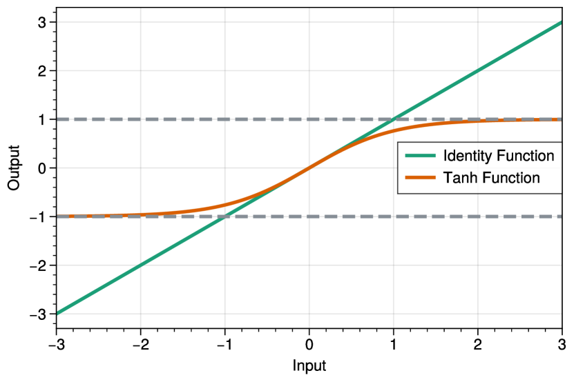
Figure 1: Comparison of two activation functions: $\sigma(x)=x$ and $\sigma(x)=\tanh(x)$. The nonlinear activation $\tanh(\cdot)$ keeps small values while shrinking large values.

As a result, if the difference between two nodes is large, we think they are dissimilar, and then restrict the information exchange to prevent them from being undistinguished. Otherwise, if the difference is small, we tend to think they are similar, and let them exchange information like normal GCNs. In graph diffusion, this amounts to a desirable anisotropic-like behavior that adaptively aggregates more from similar neighbors and less from dissimilar neighbors, which helps prevent over-smoothing and improves robustness to noisy perturbations. Besides, our graph diffusion resembles the well-known PM diffusion (Perona & Malik, 1990), which is a well-known adaptive diffusion used in image processing to preserve desired image structures, such as edges, while blurring others. To achieve this, they manually design a nonlinear function that approximates an impulse function close to edges to reweight the differences between image pixels. Compared with them, our nonlinear diffusion with the linear operator ${\mathcal{K}}$ allows us to parameterize a flexible and learnable aggregation function.

3.2 Proposed GIND

The discussion above shows that our nonlinear diffusion is a principled generalization of previous linear isotropic diffusion with beneficial anisotropic properties. In this part, we apply it on the graph data and develop the corresponding implicit graph neural networks.

Nonlinear Diffusion on Graphs. As known in previous literature (Chung & Graham, 1997), the differential operators could be instantiated on a discrete graph ${\mathcal{G}}$ with $n$ nodes and $m$ edges, and each node contains $h$-dimensional features. Specifically, let $\mathbf{U}\in{\mathbb{R}}^{n\times h}$ be the feature matrix, the gradient operator $\nabla$ corresponds to the incidence matrix $\mathbf{G}\in{\mathbb{R}}^{m\times n}$. It is defined as $\mathbf{G}_{k,i}=1$ if edge $k$ enters node $i$, $-1$ if it leaves node $i$, and $0$ otherwise. The divergence operator, the negative of which is the adjoint of the gradient operator, now corresponds to $-\mathbf{G}^{\top}\in{\mathbb{R}}^{n\times m}$. The linear operator ${\mathcal{K}}$ corresponds to a feature transformation matrix $\mathbf{K}\in{\mathbb{R}}^{h\times h}$, and its adjoint ${\mathcal{K}}^{\star}$ becomes $\mathbf{K}^{\top}$. As a result, the nonlinear diffusion in Equation 3 has the following matrix form on graph ${\mathcal{G}}$,

$$\partial_{t}\mathbf{U}=-\mathbf{G}^{\top}\sigma(\mathbf{G}\mathbf{U}\mathbf{K}^{\top})\mathbf{K}.$$ (8)

Following the analysis above, we choose the activation function $\sigma(x)=\tanh(x)$. A more detailed derivation can be found in Appendix B.

Our Implicit GNNs. By adopting the nonlinear graph diffusion developed above for the implicit graph diffusion mechanism, we develop a new implicit GNN, Graph Implicit Nonlinear Diffusion (GIND), with the following formulation,

$$\mathbf{Z} =-\hat{\mathbf{G}}^{\top}\sigma(\hat{\mathbf{G}}(\mathbf{Z}+b_{\bm{\Omega}}(\mathbf{X}))\mathbf{K}^{\top})\mathbf{K},$$ (9a)

$$\hat{\mathbf{Y}} =g_{\bm{\Theta}}(\mathbf{X}+\mathbf{Z}),$$ (9b)

where $\hat{\mathbf{G}}=\mathbf{G}\tilde{\mathbf{D}}^{-1/2}/\sqrt{2}$ is the normalized incidence matrix. Here, we first embed the input feature matrix $\mathbf{X}$ with an affine transformation $b_{\bm{\Omega}}(\cdot)$ with parameters $\bm{\Omega}$. Then, the input embedding is injected to the implicit diffusion layer, whose output $\mathbf{Z}$ is the equilibrium of a nonlinear fixed point equation (Equation 9a). Afterwards, we use $\mathbf{X}+\mathbf{Z}$, the sum of the input features (initial value) and the equilibrium (the flux), as the final value to predict the labels. The readout head $g_{\bm{\Theta}}$ can be parametrized by a linear layer or an MLP. We also provide a row-normalized variant of the initial formulation (Equation 9a) in Appendix D.

Notably, in GIND, we design the equilibrium states $\mathbf{Z}$ to be the residual refinement of the input features $\mathbf{X}$ through the diffusion process, a.k.a. the transported mass of $\mathbf{X}$ (Weickert, 1998). As a result, starting from an initial value, the estimated transported mass $\mathbf{Z}$ could be gradually refined through the fixed point iteration of our nonlinear diffusion process. Finally, it will reach a stable equilibrium $\mathbf{Z}$ that cannot be further improved.

As an implicit model, our GIND enjoys the benefits of general implicit GNNs, including the ability to capture long-range dependencies as well as constant memory footprint. With our proposed nonlinear diffusion mechanism, it could adaptively aggregate useful features from similar neighbors and filter out noisy ones. Last but not least, as we show in the next section, the equilibrium states of our GIND can be formalized as the solution of a convex objective.

4 An Optimization Framework for GIND

In this section, inspired by recent works on optimization-based implicit models (Xie et al., 2022), we develop the first optimization framework for an implicit graph neural network. Specifically, we show that the equilibrium states of our GIND correspond to the solution of a convex objective. Based on this property, we show that we can derive principled variants of GIND through various regularization terms, which demonstrates a principled way to inject inductive bias into the model representations.

4.1 Formulation of Structural Objective

Notations. We use $\otimes$ to represent the Kronecker product, and use $\odot$ to represent element-wise product. For a matrix $\mathbf{W}\in{\mathbb{R}}^{p\times q}$, ${\bm{w}}=\textup{\mbox{vec}}(\mathbf{W})$ represents the vectorized form of $\mathbf{W}$ obtained by stacking its columns. We use $\left\|\cdot\right\|_{2}$ for the matrix operator norm and $\left\|\cdot\right\|$ for the vector $\ell_{2}$-norm. A function $f:\mathcal{H}\to\mathbb{R}\cup\{+\infty\}$ is proper if the set $\{{\bm{x}}:f({\bm{x}})<+\infty\}$ is non-empty, where $\mathcal{H}$ is the Euclidean space. For a proper convex function $f:\mathcal{H}\to\mathbb{R}\cup\{+\infty\}$, its proximal operator $\text{Prox}^{\mu}_{f}({\bm{x}})$ is defined as $\{{\bm{z}}\in\mathcal{H}:{\bm{z}}=\operatorname*{arg\,min}_{{\bm{u}}}\frac{1}{2\mu}\left\|{\bm{u}}-{\bm{x}}\right\|^{2}+f({\bm{u}})\}$. We omit $\mu$ when $\mu=1$.

For convenience, from now on, we adopt an equivalent “vectorized” version of the implicit layer (Equation 9a) using Kronecker product:

$${\bm{z}}=-(\mathbf{K}\otimes\hat{\mathbf{G}})^{\top}\sigma((\mathbf{K}\otimes\hat{\mathbf{G}})({\bm{z}}+\textup{\mbox{vec}}(b_{\bm{\Omega}}({\bm{x}})))),$$ (10)

where ${\bm{z}}$ is the vectorized version of the equilibrium state $\mathbf{Z}$, and we use $f({\bm{z}})$ to denote the right-hand side.

The following theorem shows that the equilibrium states of our GIND correspond to the solution of a convex objective.

Theorem 4.1.

Assume that the nonlinear function $\sigma(\cdot)$ is monotone and $L_{\sigma}$-Lipschitz, i.e.,

$$0\leq\frac{\sigma(a)-\sigma(b)}{a-b}\leq L_{\sigma},\forall\ a,b\in\mathbb{R},a\neq b,$$ (11)

and $1\geq L_{\sigma}\left\|\mathbf{K}\otimes\hat{\mathbf{G}}\right\|_{2}^{2}=L_{\sigma}\left\|\mathbf{K}\right\|_{2}^{2}\left\|\hat{\mathbf{G}}\right\|_{2}^{2}$. Then there exists a convex function $\varphi({\bm{z}})$, such that its minimizer is the solution to the equilibrium equation ${\bm{z}}=f({\bm{z}})$. Furthermore, we have $\operatorname{Prox}_{\varphi}({\bm{z}})=\frac{1}{L_{\sigma}+1}(L_{\sigma}{\bm{z}}+f({\bm{z}}))$.

With Theorem 4.1, we can easily establish the following sufficient condition for our model to be well-posed, i.e., the existence and uniqueness of its solution, which guarantees the convergence of iterative solvers for reaching the equilibrium.

Proposition 4.2.

Our implicit layer (Equation 10) is guaranteed to be well-posed if $\left\|\mathbf{K}\right\|_{2}\|\hat{\mathbf{G}}\|_{2}<1$. Since we already have $\|\hat{\mathbf{G}}\|_{2}\leq 1$, we can fulfill the condition with $\left\|\mathbf{K}\right\|_{2}<1$.

4.2 Optimization-Inspired Variants

In previous part, we have established the structural objective of our proposed GIND. Here, we present an intriguing application of this perspective, which is to derive structural variants of our implicit model by injecting inductive bias in a principled way. Specifically, we study three examples: skip-connection induced by Moreau envelop (Xie et al., 2022), and two interpretable feature regularization: Laplacian smoothing and feature decorrelation.

Optimization-Inspired Skip-Connection. Since the equilibrium state of our implicit layer is the minimizer of an objective function $\varphi(\cdot)$, we can replace it directly with a new formula $\Phi(\cdot)$, as long as it has the same minimizer as the original one. Specifically, we choose its Moreau envelope function. Given a proper closed convex function $\varphi:\mathcal{H}\to\mathbb{R}\cup\{+\infty\}$ and $\mu>0$, the Moreau envelope of $\varphi$ is the function

$$M_{\varphi}^{\mu}({\bm{z}})=\min_{{\bm{u}}}\frac{1}{2\mu}\left\|{\bm{u}}-{\bm{z}}\right\|^{2}+\varphi({\bm{u}}),$$ (12)

which is a smoothed approximate of $\varphi(\cdot)$ (Attouch & Aze, 1993). Meanwhile, the Moreau envelope function keeps the same critical points as the original one. Its proximal operator can be computed as follows:

$$\operatorname{Prox}^{\lambda}_{M_{\varphi}^{\mu}}({\bm{z}})={\bm{z}}+\frac{\lambda}{\mu+\lambda}(\operatorname{Prox}^{\mu+\lambda}_{\varphi}({\bm{z}})-{\bm{z}}),$$ (13)

where $\lambda,\mu>0$. Letting $\lambda=\alpha$ and $\mu=1-\alpha$, we have a new implicit layer induced from its proximal operator as follows:

$${\bm{z}}=\mathcal{T}({\bm{z}})\coloneqq(1-\alpha){\bm{z}}+\alpha f({\bm{z}}),$$ (14)

where $\alpha\in(0,1]$. Empirically, skip-connection improves stability in the iteration while keeping the equilibrium unchanged.

Optimization-Inspired Feature Regularization. Regularization has become an important part of modern machine learning algorithms. Since we know the objective, we can combine it with regularizers to introduce customized properties to the equilibrium, which is equivalent to making a new implicit composite layer by appending one layer before the original implicit layer (Xie et al., 2022). Formally, if we modify $\Phi({\bm{z}})$ to $\Phi({\bm{z}})+\mathcal{R}({\bm{z}})$, then the implicit layer becomes:

$${\bm{z}}=\mathcal{T}({\bm{z}})\circ\mathcal{T}_{\mathcal{R}},$$ (15)

where $\mathcal{T}_{\mathcal{R}}=\operatorname{Prox}_{\mathcal{R}}$, and $\circ$ denotes the mapping composition. When the proximal is hard to calculate, we can use a gradient descent step as an approximate evaluation, which is $\mathcal{T}_{\mathcal{R}_{z}}\approx\mathcal{I}-\eta\frac{\partial\mathcal{R}_{z}}{\partial z}$. In general, we can instantiate $\mathcal{R}_{z}$ as any convex function that has the preferred properties of the equilibrium. Specifically, we consider two kinds of regularization.

• Laplacian Regularization. The graph Laplacian operator $\mathbf{L}=\mathbf{D}-\mathbf{A}$ is a positive semi-definite matrix (Chung & Graham, 1997). We use the (symmetric normalized) Laplacian regularization $\hat{\tilde{\mathbf{L}}}=\mathbf{I}-\hat{\tilde{\mathbf{A}}}$ to push the equilibrium of the linked nodes closer in the feature space. It is defined as follows:

  $$\mathcal{R}_{\operatorname{Lap}}({\bm{z}})={\bm{z}}^{\top}\tilde{\mathbf{D}}^{-\frac{1}{2}}L\tilde{\mathbf{D}}^{-\frac{1}{2}}{\bm{z}}=\left\|\hat{\mathbf{G}}{\bm{z}}\right\|^{2}.$$ (16)

• Feature Decorrelation. We use the feature decorrelation regularization to reduce redundant information between feature dimensions (Rodríguez et al., 2017; Ayinde et al., 2019). It is defined as follows:

  $$\mathcal{R}_{\operatorname{Dec}}({\bm{z}})=\frac{1}{2}\left\|\hat{{\bm{z}}}\hat{{\bm{z}}}^{\top}-\mathbf{I}\right\|_{F}^{2},$$ (17)

  where $\hat{{\bm{z}}}$ is the normalized ${\bm{z}}$.

5 Efficient Training of GIND

Training stability has been a widely existing issue for general implicit models (Bai et al., 2019; Geng et al., 2021; Li et al., 2022b) as well as implicit GNNs (Gu et al., 2020). To train our GIND, we adopt an efficient training strategy that works effectively in our experiments.

Forward and Backward Computation. Specifically, in the forward pass, we adopt the fixed point iteration as in Gu et al. (2020); while in the backward pass, we adopt the recently developed Phantom Gradient (Geng et al., 2021) estimation, which enjoys both efficient computation and stable training dynamics.

Variance Normalization. In previous implicit models (Bai et al., 2019, 2020), LayerNorm (Ba et al., 2016) is often applied on the output features to enhance the training stability of implicit models. Specifically, for GIND, we apply normalization before the nonlinear activation $\sigma(\cdot)$ and drop the mean items to keep it a sign-preserving transformation:

$$\operatorname{norm}({\bm{v}})=\frac{{\bm{v}}}{\sqrt{\mathrm{Var}({\bm{v}})+\varepsilon}}\odot\bm{\gamma},$$ (18)

where $\bm{\gamma}>0$ denotes positive scaling parameters and $\varepsilon$ is a small constant. As discussed in previous works (Zhou et al., 2021), this could effectively prevent the variance inflammation issue and help stabilize the training process with increasing depth.

Table 1: Results on heterophilic node classification datasets: mean accuracy (%) $\pm$ standard deviation over different data splits.

Type	Method	Cornell	Texas	Wisconsin	Chameleon	Squirrel
	GCN	59.19$\pm$3.51	64.05$\pm$5.28	61.17$\pm$4.71	42.34$\pm$2.77	29.0$\pm$1.10
	GAT	59.46$\pm$6.94	61.62$\pm$5.77	60.78$\pm$8.27	46.03$\pm$2.51	30.51$\pm$1.28
	JKNet	58.18$\pm$3.87	63.78$\pm$6.30	60.98$\pm$2.97	44.45$\pm$3.17	30.83$\pm$1.65
Explicit	APPNP	63.78$\pm$5.43	64.32$\pm$7.03	61.57$\pm$3.31	43.85$\pm$2.43	30.67$\pm$1.06
	Geom-GCN	60.81	67.57	64.12	60.9	38.14
	GCNII	76.75$\pm$5.95	73.51$\pm$9.95	78.82$\pm$5.74	48.59$\pm$1.88	32.20$\pm$1.06
	H2GCN	82.22$\pm$5.67	84.76$\pm$5.57	85.88$\pm$4.58	60.30$\pm$2.31	40.75$\pm$1.44
	IGNN	61.35$\pm$4.84	58.37$\pm$5.82	53.53$\pm$6.49	41.38$\pm$2.53	24.99$\pm$2.11
Implicit	EIGNN	85.13$\pm$5.57	84.60$\pm$5.41	86.86$\pm$5.54	62.92$\pm$1.59	46.37$\pm$1.39
	GIND (ours)	85.68$\pm$3.83	86.22$\pm$5.19	88.04$\pm$3.97	66.82$\pm$2.37	56.71$\pm$2.07

6 Comparison to Related Work

Here, we highlight the contributions of our proposed GIND through a detailed comparison to related work, including implicit GNNs and explicit GNNs.

6.1 Comparison to Implicit GNNs

Diffusion Process. Prior to our work, IGNN (Gu et al., 2020) and EIGNN (Liu et al., 2021a) adopt the same aggregation mechanism as GCN (Kipf & Welling, 2016), which is equivalent to an isotropic linear diffusion that is irrelevant to neighbor features (Wang et al., 2021). CGS (Park et al., 2021) instead uses a learnable aggregation matrix to replace the original normalized adjacency matrix. However, the aggregation matrix is fixed in the implicit layer, thus the diffusion process still cannot adapt to the iteratively updated hidden states. In comparison, we design a nonlinear diffusion process with anisotropic properties. As a result, it is adaptive to the updated features and helps prevent over-smoothing. An additional advantage of GIND is that we can deduce its equilibrium states from a convex objective in a principled way, while in previous works the implicit layers are usually heuristically designed.

Training. IGNN (Gu et al., 2020) adopts projected gradient descent to limit the parameters to a restricted space at each optimization step, which, still occasionally experiences diverged iterations. EIGNN (Liu et al., 2021a) and CGS (Park et al., 2021) resort to linear implicit layers and reparameterization tricks to derive a closed-form solution directly, however, at the cost of degraded expressive power compared to nonlinear layers. In our GIND, we instead enhance the model expressiveness with our proposed nonlinear diffusion. During training, we regularize the forward pass with variance normalization and adopt the Phantom Gradient (Geng et al., 2021) to obtain a fast and robust gradient estimate.

6.2 Comparison to Explicit GNNs

Diffusion-Inspired GNNs. Diffusion process has also been applied to design explicit GNNs. Atwood & Towsley (2016) design multi-hop representations from a diffusion perspective. Xhonneux et al. (2020) address continuous message passing based on a linear diffusion PDE. Wang et al. (2021) point out the equivalence between GCN propagation and the numerical discretization of an isotropic diffusion process, and achieve better performance by further decoupling the terminal time and the propagation steps. Chamberlain et al. (2021) also explore different numerical discretization schemes. They develop models based on both linear and nonlinear diffusion equations. However, their nonlinear counterpart does not outperform the linear one. Eliasof et al. (2021) resort to alternative dynamics, including a diffusion process and a hyperbolic process, and design two corresponding models. In comparison, our GIND replaces the explicit diffusion discretization with an implicit formulation. The implicit formulation admits an equilibrium that corresponds to infinite diffusion steps, through which we enlarge the receptive field while being free from manual tuning of the terminal time and the step size of the diffusion equation.

Optimization-Inspired GNNs. Prior to our work, there have been many works (Zhu et al., 2021; Yang et al., 2021; Ma et al., 2021; Liu et al., 2021b) that establish a connection between different linear propagation schemes and the graph signal denoising with Laplacian smoothing regularization. By modifying the objective function, Zhu et al. (2021) introduce adjustable graph kernels with different low-pass and high-pass filtering capabilities, Ma et al. (2021) introduce a model that regularizes each node with different regularization strength, and Liu et al. (2021b) enhance the local smoothness adaptivity of GNNs by replacing the $\ell_{2}$ norm by $\ell_{1}$-based graph smoothing. Yang et al. (2021) focus on the iterative algorithms used to solve the objective, and introduce a model inspired by unfolding optimization iterations of the objective function. Their discussions are all limited to explicit layers and ignore the (potentially nonlinear) feature transformation steps. In comparison, our GIND discusses implicit layers, and admits a unified objective of both the nonlinear diffusion step and the transformation step. Besides, optimization-inspired explicit GNNs usually model a single iteration step, while our implicit model ensures that the obtained equilibrium is exactly the solution to the corresponding objective.

7 Experiments

In this section, we conduct a comprehensive analysis on GIND and compare it against both implicit and explicit GNNs on various problems and datasets. We refer to Appendix E for the details of the data statistics, network architectures and training details. We implement our GIND based on the PyTorch Geometric library (Fey & Lenssen, 2019). Our code is available at https://github.com/7qchen/GIND.

7.1 Performance on Node Classification

Table 2: Results on homophilic node classification datasets: mean accuracy (%).

Type	Method	Cora	CiteSeer	PubMed
	GCN	85.77	73.68	88.13
	GAT	86.37	74.32	87.62
	JKNet	85.25	75.85	88.94
Explicit	APPNP	87.87	76.53	89.40
	Geom-GCN	85.27	77.99	90.05
	GCNII	88.49	77.08	89.57
	H2GCN	87.87	77.11	89.49
	IGNN*	85.80	75.24	87.66
Implicit	EIGNN*	85.89	75.31	87.92
	GIND (ours)	88.25	76.81	89.22

Table 3: Results of micro-averaged F$1$ score on PPI dataset.

Type	Method	Micro-F1
	GCN	59.2
	GAT	97.3
Explicit	GraphSAGE	78.6
	JKNet	97.6
	GCNII	99.5
	IGNN	97.0
Implicit	EIGNN	98.0
	GIND (ours)	98.4

Table 4: Results of graph classification: mean accuracy (%) $\pm$ standard deviation over 10 random data splits.

Type	Method	MUTAG	PTC	COX2	PROTEINS	NCI1
	WL	84.1$\pm$1.9	58.0$\pm$2.5	83.2$\pm$0.2	74.7$\pm$0.5	84.5$\pm$0.5
	DCNN	67.0	56.6	-	61.3	62.6
Explicit	DGCNN	85.8	58.6	-	75.5	74.4
	GIN	89.4$\pm$5.6	64.6$\pm$7.0	-	76.2$\pm$2.8	82.7$\pm$1.7
	FDGNN	88.5$\pm$3.8	63.4$\pm$5.4	83.3$\pm$2.9	76.8$\pm$2.9	77.8$\pm$1.6
	IGNN*	76.0$\pm$13.4	60.5$\pm$6.4	79.7$\pm$3.4	76.5$\pm$3.4	73.5$\pm$1.9
Implicit	CGS	89.4$\pm$5.6	64.7$\pm$6.4	-	76.3$\pm$4.9	77.6$\pm$2.0
	GIND (ours)	89.3$\pm$7.4	66.9$\pm$6.6	84.8$\pm$4.2	77.2$\pm$2.9	78.8$\pm$1.7

Datasets. We test GIND against the selected set of baselines for node classification task. We adopt the $5$ heterophilic datasets: Cornell, Texas, Wisconsin, Chameleon and Squirrel (Pei et al., 2019). And for homophilic datasets, we adopt $3$ citation datasets: Cora, CiteSeer and PubMed. We also evaluate GIND on PPI to show that GIND is applicable to multi-label multi-graph inductive learning. For other datasets except PPI, we adopt the standard data split as Pei et al. (2019) and report the average performance over the $10$ random splits. While for PPI, we follow the train/validation/test split used in GraphSAGE (Hamilton et al., 2017).

Baselines. Here, we compare our approach against several representative explicit and implicit methods that also adopt the same data splits. For explicit models, we select several representative baselines to compare, i.e., GCN (Kipf & Welling, 2016), GAT (Veličković et al., 2017), JKNet (Xu et al., 2018), APPNP (Klicpera et al., 2018), Geom-GCN (Pei et al., 2019), GCNII (Chen et al., 2020), and H2GCN (Zhu et al., 2020). For Geom-GCN, we report the best result among its three model variants. For implicit methods, we present the results of IGNN (Gu et al., 2020) and EIGNN (Liu et al., 2021a). We implement IGNN on citation datasets with their $1$-layer model used for node classification, and implement EIGNN on citation datasets with their model used for heterophilic datasets. We mark the results implemented by us with $*$. We do not include CGS (Park et al., 2021), as they do not introduce a model for node-level tasks.

Results. As shown in Table 1, our model outperforms the explicit and implicit baselines on all heterophilic datasets by a significant margin, especially on the larger datasets Chameleon and Squirrel. In particular, we improve the current state-of-the-art accuracy of EIGNN from $46.37\%$ to $56.71\%$ on the Squirrel dataset, while the state-of-the-art explicit model H2GCN only reaches $40.75\%$ accuracy. Among explicit models, JKNet, APPNP and GCNII are either designed to consider a larger range of neighbors or to mitigate oversmoothing. Despite that they outperform GCN and GAT, they still perform worse than implicit models on most datasets. Compared to other implicit models (EIGNN and IGNN), GIND still shows clear advantages. Consequently, we argue that the success of our network stems not only from the implicit setting, but also from our nonlinear diffusion that enhances useful features in aggregation.

Also, our results in Table 2 show that GIND achieves similar accuracy to the compared methods on $3$ citation datasets, although they may not need as many long-range dependencies as the heterophilic datasets. On the PPI dataset, as depicted from Table 3, our GIND achieves $98.4$ micro-averaged F$1$ score, still superior to other implicit methods and most explicit methods, close to the state-of-the-art models. Moreover, with a small initialization for the parameters, all our training processes are empirically stable.

7.2 Performance on Graph Classification

Datasets. For graph classification, we choose a total of $5$ bioinformatics benchmarks: MUTAG, PTC, COX2, NCI1 and PROTEINS (Yanardag & Vishwanathan, 2015). Following identical settings as Yanardag & Vishwanathan (2015), we conduct $10$-fold cross-validation with LIB-SVM (Chang & Lin, 2011) and report the average prediction accuracy and standard deviations in Table 4.

Baselines. Here, we include the baselines that also have reported results on the chosen datasets. For explicit models, we choose Weisfeiler-Lehman Kernel (WL) (Shervashidze et al., 2011), DCNN (Atwood & Towsley, 2016), DGCNN (Zhang et al., 2018), GIN (Xu et al., 2018) and FDGNN (Gallicchio & Micheli, 2020). For implicit models, we reproduce the result of IGNN (Gu et al., 2020) with their source code for a fair comparison, since it used a different performance metric. We mark the results implemented by us with $*$. We do not include EIGNN (Liu et al., 2021a), as they do not introduce a model for graph-level tasks.

Results. In this experiment, GIND achieves the best performance in $3$ out of $5$ experiments given the competitive baselines. Such performance further validates GIND’s success that it can still capture long-range dependencies when generalized to unseen testing graphs. Note that GIND also outperforms both implicit baselines.

7.3 Empirical Understandings of GIND

Table 5: Comparison of different regularization types.

Reg	Cora	CiteSeer	PubMed
None	88.25$\pm$1.25	76.81$\pm$1.68	89.22$\pm$0.40
$\mathcal{R}_{\operatorname{Lap}}$	88.33$\pm$1.15	76.95$\pm$1.73	89.42$\pm$0.50
$\mathcal{R}_{\operatorname{Dec}}$	88.29$\pm$0.92	76.84$\pm$1.70	89.28$\pm$0.41

Feature Regularization. In this experiment, we compare the performance of two kinds of feature regularization: the Laplacian regularization $\mathcal{R}_{\operatorname{Lap}}$ and the feature decorrelation $\mathcal{R}_{\operatorname{Dec}}$. We use the $3$ citation dataset for comparison. We choose an appropriate regularization coefficient $\eta$ for each dataset. As reported in Table 5, Laplacian regularization improves the performance for the homophilic datasets. We attribute this to the fact that similarity between nodes is an appropriate assumption for these datasets. The feature decorrelation also improves the performance slightly.

Long-Range Dependencies. We follow Gu et al. (2020) and use the synthetic dataset Chains to evaluate models’ abilities for capturing long-range dependencies. The goal is to classify nodes in a chain of length $l$, whose label information is only encoded in the starting end node. We use the same experimental settings as IGNN and EIGNN. We show in Figure 2 the experimental results with chains of different lengths. In general, the implicit models all outperform the explicit models for longer chains, verifying that they have advantages for capturing long-range dependencies. GIND and EIGNN both repetitively maintain $100\%$ test accuracy with the length of $200$. While EIGNN only applies to linear cases, GIND can apply to more general nonlinear cases.

Table 6: Comparison of training time on the PubMed dataset.

Method	Preprocessing	Training	Total
IGNN	0	83.67 s	83.67 s
EIGNN	1404.45 s	69.14 s	1473.59 s
CGS	0	118.65 s	118.65 s
GIND (ours)	0	47.31 s	47.31 s

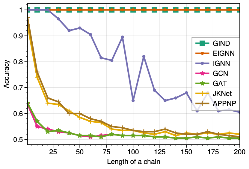
Figure 2: Average accuracy with respect to the length of chains.

Training Time. To investigate the training time, we train the $1$-layer models on PubMed dataset for $500$ epochs to compare their efficiency. Since we use gradient estimate for training, our model can be faster than those implicit models that compute exact gradients. As shown in Table 6, our model costs much fewer time ($47.31$ s) than the three models that calculate exact gradients. Among the three models, EIGNN is the most efficient with $69.14$ s training cost, but its pre-processing costs much more than training.

Table 7: Comparison of linear and nonlinear diffusion in GIND.

Dataset	CiteSeer	Cornell	Wisconsin
Linear	76.62$\pm$1.51	83.24$\pm$6.82	84.31$\pm$4.30
Nonlinear	76.81$\pm$1.68	85.58$\pm$3.83	88.04$\pm$3.97
Linear	18.60s	19.94s	20.52s
Nonlinear	20.44s	20.21s	21.30s

Efficacy of Nonlinear Diffusion. We conduct an ablation of the proposed nonlinear diffusion by removing the nonlinearity in Equation 9a. From Table 7, we can see that the nonlinear diffusion has a clear advantage over linear ones, especially on heterophilic datasets. Meanwhile, the additional computation overhead brought by the nonlinear setting is almost neglectable.

Gradient Estimate. In the left plot of Figure 3, we compare results with different backpropagation steps $L$ of Phantom Gradient (Geng et al., 2021) along with their corresponding training time on the Cora dataset. We can see that there is a tradeoff between different steps, that either too large or too small an $L$ leads to degraded performance, and the sweet spot lies in $L=4$. The corresponding training time is $15.52$ s, which is still preferable to other implicit GNNs (Table 6).

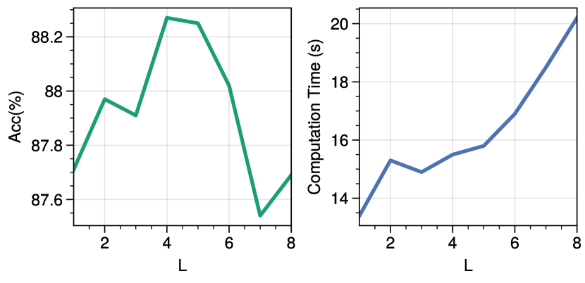
Figure 3: Left: test accuracy (%) with increasing backpropagation steps $L$ on Cora. Right: the corresponding training time (s).

8 Conclusion

In this paper, we develop GIND, an optimization-induced implicit graph neural network, which has access to infinite hops of neighbors while adaptively aggregating features with nonlinear diffusion. We characterize the equilibrium of our implicit layer from an optimization perspective, and show that the learned representation can be formalized as the minimizer of an explicit convex optimization objective. Benefiting from this, we can embed prior properties to the equilibrium and introduce skip connections to promote training stability. Extensive experiments have shown that compared with previous implicit GNNs, our GIND obtains state-of-the-art performance on various benchmark datasets.

Appendix A Kronecker Product

Given two matrices $\mathbf{A}\in\mathbb{R}^{m\times n}$ and $\mathbf{B}\in\mathbb{R}^{p\times q}$, the Kronecker product $\mathbf{A}\otimes\mathbf{B}\in\mathbb{R}^{pm\times qn}$ is defined as follows:

$$\mathbf{A}\otimes\mathbf{B}=\begin{pmatrix}\mathbf{A}_{11}\mathbf{B}&\cdots&\mathbf{A}_{1n}\mathbf{B}\\ \vdots&\ddots&\vdots\\ \mathbf{A}_{m1}\mathbf{B}&\cdots&\mathbf{A}_{mn}\mathbf{B}\end{pmatrix}.$$ (19)

By definition of the Kronecker product, we have the following important properties of the vectorization with the Kronecker product:

• $\left\|\mathbf{A}\otimes\mathbf{B}\right\|=\left\|\mathbf{A}\right\|\left\|\mathbf{B}\right\|$,

• $(\mathbf{A}\otimes\mathbf{B})^{\top}=\mathbf{A}^{\top}\otimes\mathbf{B}^{\top}$,

• $\textup{\mbox{vec}}(\mathbf{A}\mathbf{B}\mathbf{C})=(\mathbf{C}^{\top}\otimes\mathbf{A})\textup{\mbox{vec}}(\mathbf{B})$.

Appendix B Choice of the Nonlinear Transformation $\sigma(\cdot)$

Oriented Incidence Matrix on Undirected Graphs. If $\mathcal{G}$ is undirected, we randomly assign an orientation for each edge to construct an oriented incidence matrix $\mathbf{G}$, then it is unique to the obtained directed edge set $\tilde{\mathcal{E}}$. Given $\mathbf{U}\in\mathbb{R}^{n\times p}$ as the discrete version of ${\bm{u}}$, the gradient operator $(\mathbf{G}\mathbf{U})_{k,\cdot}={\bm{u}}_{j}-{\bm{u}}_{i}$ assigns the edge $k=(i,j)\in\tilde{\mathcal{E}}$ the difference of its endpoint features. Similarly, the divergence operator $-\mathbf{G}^{\top}$ assigns each node the sum of the features of all edges it shares.

To ensure the discretization of the nonlinear diffusion is well-defined for undirected graphs, we need to ensure that randomly switching the direction of the edge would not influence the output. As a result, we make the following assumption.

Assumption B.1.

The nonlinear function $\sigma(\cdot)$ is odd, i.e., $\sigma(-x)=-\sigma(x)$.

Switching the direction of an edge $k=(i,j)$ is equivalent to multiplying a matrix $\mathbf{E}_{k}$ to the left of $\mathbf{G}$, where $\mathbf{E}_{k}$ is obtained by switching the $(k,k)$-th element of an identity matrix to $-1$. If B.1 holds, we have

$$\partial_{t}\mathbf{U} =-(\mathbf{E}_{k}\mathbf{G})^{\top}\sigma(\mathbf{E}_{k}\mathbf{G}\mathbf{U}\mathbf{K}^{\top})\mathbf{K},$$ (20)

$$=-\mathbf{G}^{\top}\mathbf{E}_{k}^{\top}\mathbf{E}_{k}\sigma(\mathbf{G}\mathbf{U}\mathbf{K}^{\top})\mathbf{K},$$ (21)

$$=-\mathbf{G}^{\top}\sigma(\mathbf{G}\mathbf{U}\mathbf{K}^{\top})\mathbf{K}.$$ (22)

Consequently, the discretization is well-defined for undirected graphs.

Besides B.1, as discussed in Theorem 4.1, we need B.2 to hold. Overall, $\tanh$ satisfies both assumptions, and has an effect to keep more small gradients while shrinking large gradients.

Assumption B.2.

The nonlinear function $\sigma(\cdot)$ is monotone and $L_{\sigma}$-Lipschitz, i.e.,

$$0\leq\frac{\sigma(a)-\sigma(b)}{a-b}\leq L_{\sigma},\forall a,b\in\mathbb{R},a\neq b.$$ (23)

Appendix C Proofs

C.1 Conditions to be a Proximal Operator

Lemma C.1.

(modified version of Prop. 2 in Gribonval & Nikolova (2020)). Consider $f:\mathcal{H}\to\mathcal{H}$ defined everywhere. The following properties are equivalent:

1. there is a proper convex l.s.c function $\varphi:\mathcal{H}\to\mathbb{R}\cup\{+\infty\}$ s.t. $f({\bm{z}})\in\operatorname{Prox}_{\varphi}({\bm{z}})$ for each ${\bm{z}}\in\mathcal{H}$;
   

2. the following conditions hold jointly:

   1. there exists a convex l.s.c function $\psi:\mathcal{H}\to\mathbb{R}$ s.t. $\forall\mathbf{y}\in\mathcal{H},f(\mathbf{y})=\nabla\psi(\mathbf{y})$;

   2. $\left\|f(\mathbf{y})-f(\mathbf{y}^{\prime})\right\|\leq\left\|\mathbf{y}-\mathbf{y}^{\prime}\right\|,\forall\mathbf{y},\mathbf{y}^{\prime}\in\mathcal{H}$.

There exists a choice of $\varphi(\cdot)$ and $\psi(\cdot)$, satisfying (i) and (ii), such that $\varphi({\bm{z}})=\psi^{*}({\bm{z}})-\frac{1}{2}\left\|{\bm{z}}\right\|^{2}$.

Proof.

(i) $\Rightarrow$ (ii): Since $\varphi({\bm{x}})+\frac{1}{2}\left\|{\bm{x}}\right\|^{2}$ is a proper l.s.c $1$-strongly convex function, then by Thm. 5.26 in Beck (2017), its conjugate function $f^{*}(\mathbf{y})=\sup\{\langle\mathbf{y},{\bm{x}}\rangle-f({\bm{x}}):{\bm{x}}\in\mathcal{H}\}$ is $\frac{1}{\sigma}$-smooth when $f$ is proper, closed and $\sigma$ strongly convex and vice versa. Thus, we have:

$$\psi({\bm{x}})\coloneqq[\varphi({\bm{x}})+\frac{1}{2}\left\|{\bm{x}}\right\|^{2}]^{*},$$ (24)

is $1$-smooth with $\operatorname{dom}(\psi)=\mathcal{H}$. Then we get:

$$f({\bm{x}}) \in\operatorname*{arg\,min}_{\bm{u}}\frac{1}{2}\left\|{\bm{u}}-{\bm{x}}\right\|^{2}+\varphi({\bm{u}})=\{{\bm{u}}:{\bm{x}}\in\partial\varphi({\bm{u}})+{\bm{u}}\},$$ (25)

$$=\{{\bm{u}}|{\bm{x}}\in\partial(\varphi({\bm{u}})+\frac{1}{2}\left\|{\bm{u}}\right\|^{2})\},$$ (26)

$$=\{{\bm{u}}|{\bm{u}}=\nabla\psi({\bm{x}})\}=\{\nabla\psi({\bm{x}})\}.$$ (27)

Hence $f({\bm{x}})=\nabla\psi({\bm{x}})$, and $1$-smoothness of $\psi$ implies $f$ is nonexpansive.

(ii) $\Rightarrow$ (i): Let $\varphi({\bm{x}})=\psi^{*}({\bm{x}})-\frac{1}{2}\left\|{\bm{x}}\right\|^{2}$. Since $\psi({\bm{x}})$ is $1$-smooth, similarly we can conclude: $\psi^{*}$ is $1$-strongly convex. Hence, $\varphi$ is convex, and:

$$\operatorname{Prox}_{\varphi}({\bm{x}}) =\operatorname*{arg\,min}_{{\bm{u}}}\{\frac{1}{2}\left\|{\bm{u}}-{\bm{x}}\right\|^{2}+\varphi({\bm{u}})\},$$ (28)

$$=\{{\bm{u}}|{\bm{x}}\in\partial\varphi({\bm{u}})+{\bm{u}}\},$$ (29)

$$=\{\nabla\psi({\bm{x}})\}=\{f({\bm{x}})\},$$ (30)

which means $f({\bm{x}})=\operatorname{Prox}_{\varphi}({\bm{x}})$. ∎

C.2 Proof of Theorem 4.1

The proof follows the one presented in Xie et al. (2022).

Proof.

The equation ${\bm{z}}=f({\bm{z}})$ can be reformulated as

$${\bm{z}}+L_{\sigma}{\bm{z}}=L_{\sigma}{\bm{z}}+f({\bm{z}})\Longleftrightarrow{\bm{z}}=g({\bm{z}})\coloneqq\frac{1}{L_{\sigma}+1}(L_{\sigma}{\bm{z}}+f({\bm{z}})).$$ (31)

In the proof, without loss of generality, we let $L_{\sigma}=1$. Since $\sigma(a)$ is a single-valued function with slope in $[0,1]$, the element-wise defined operator $\sigma(a)$ is nonexpansive. Combining with $\left\|\mathbf{K}\otimes\hat{\mathbf{G}}\right\|\leq 1$, operator $f({\bm{z}})$ is nonexpansive, and $g({\bm{z}})$ is also nonexpansive by definition.

Let $\tilde{\sigma}(a)=\int_{0}^{a}\sigma(t)dt$ be a function applied element-wisely to $\forall a\in\mathbb{R}$, and $\mathbf{1}$ is the all one vector. Since $\mathbf{1}^{\top}\tilde{\sigma}(\mathbf{y})=\sum_{i=1}^{n}\tilde{\sigma}(y_{i})$, we have $\nabla\tilde{\sigma}(\mathbf{y})=[\sigma(y_{1}),\cdots,\sigma(y_{n})]^{\top}=\sigma(\mathbf{y})$. Let $\psi({\bm{z}})=\frac{1}{4}\left\|{\bm{z}}\right\|^{2}-\frac{1}{2}\mathbf{1}^{\top}\tilde{\sigma}((\mathbf{K}\otimes\hat{\mathbf{G}})({\bm{z}}+\textup{\mbox{vec}}(b_{\bm{\Omega}}({\bm{x}}))))$, by the chain rule, $\nabla\psi({\bm{z}})=\frac{1}{2}{\bm{z}}-\frac{1}{2}(\mathbf{K}\otimes\hat{\mathbf{G}})^{\top}\sigma((\mathbf{K}\otimes\hat{\mathbf{G}})({\bm{z}}+\textup{\mbox{vec}}(b_{\bm{\Omega}}({\bm{x}}))))=g({\bm{z}})$. Due to Lemma C.1, we have $g({\bm{z}})=\operatorname{Prox}_{\varphi}({\bm{z}})$, where $\varphi({\bm{z}})$ can be chosen as $\psi^{*}({\bm{z}})-\frac{1}{2}\left\|{\bm{z}}\right\|^{2}$. As a result, the solution to the equilibrium equation ${\bm{z}}=f({\bm{z}})$ is the minimizer of the convex function $\varphi(\cdot)$. ∎

Appendix D Row-Normalization Variant of GIND

Considering numerical stability, we impose the symmetric normalization to the incidence matrix in our implicit layer (Equation 9a), which is widely used in GNN models. Alternatively, we provide a row-normalization variant as follows.

$$\mathbf{Z}=-(2\tilde{\mathbf{D}})^{-1}\mathbf{G}^{\top}\sigma(\mathbf{G}(\mathbf{Z}+b_{\bm{\Omega}}(\mathbf{X}))\mathbf{K}^{\top})\mathbf{K}.$$ (32)

Note that the two formulations are equivalent in the sense that Equation 32 can be rewritten as the following formulation:

$$\bar{\mathbf{Z}}=-\hat{\mathbf{G}}^{\top}\sigma(\hat{\mathbf{G}}(\bar{\mathbf{Z}}+\bar{b}_{\bm{\Omega}}(\mathbf{X}))\mathbf{K}^{\top})\mathbf{K},$$ (33)

where $\bar{\mathbf{Z}}=(2\tilde{\mathbf{D}})^{\frac{1}{2}}\mathbf{Z}$ and $\bar{b}_{\bm{\Omega}}(\mathbf{X})=(2\tilde{\mathbf{D}})^{\frac{1}{2}}b_{\bm{\Omega}}(\mathbf{X})$. Moreover, without changing the output $\mathbf{Y}$, the row-normalized version of GIND has the following formulation:

$$\bar{\mathbf{Z}} =-\hat{\mathbf{G}}^{\top}\sigma(\hat{\mathbf{G}}(\bar{\mathbf{Z}}+\bar{b}_{\bm{\Omega}}(\mathbf{X}))\mathbf{K}^{\top})\mathbf{K},$$ (34a)

$$\mathbf{Y} =g_{\bm{\Theta}}(\mathbf{X}+(2\tilde{\mathbf{D}})^{-\frac{1}{2}}\bar{\mathbf{Z}}).$$ (34b)

Without loss of generality, all the results can be easily adapted to the row-normalization case.

Appendix E More on Experiments

E.1 Datasets

The statistics for the datasets used in node-level tasks is listed in Table 8. Among heterophilic datasets, Cornell, Texas and Wisconsin are web-page graphs of the corresponding universities, while Chameleon and Squirrel are web-page graphs of Wikipedia of the corresponding topic. The node features are bag-of-word representations of informative nouns in the web-pages. Among homophilic datasets, PPI contains multiple graphs where nodes are proteins and edges are interactions between proteins. The statistics for the datasets used in graph-level tasks is listed in Table 9. All these datasets consist of chemical molecules where nodes refer to atoms while edges refer to atomic bonds.

Table 8: Dataset statistics for node classification task.

Dataset	Cornell	Texas	Wisconsin	Chameleon	Squirrel	Cora	CiteSeer	PubMed
Nodes	1,283	183	251	2,277	5,201	2,708	3,327	19,717
Edges	280	295	466	31,421	198,493	5429	4732	44338
Features	1,703	1,703	1,703	2,325	2,089	1433	3703	500
Classes	5	5	5	5	5	7	6	3

Table 9: Dataset statistics for graph classification task.

Dataset	MUTAG	PTC	COX2	PROTEINS	NCI1
# graphs	188	344	467	1,113	4,110
Avg # nodes	17.9	25.5	41.2	39.1	29.8
Classes	2	2	2	2	2

E.2 Model Architectures

In terms of model variants, we use symmetric normalized GIND for the PPI, Chameleon and Squirrel datasets, and row-normalized GIND for the other datasets. We use a $4$-layer model for PPI and a $3$-layer model for the two large datasets, Chameleon and Squirrel, as well as all the datasets used for graph-level tasks. For the rest datasets, we adopt the model with only one layer. We use linear output function for all the node-level tasks, and MLP for all the graph-level tasks. We adopt the layer normalization (LN) (Ba et al., 2016) for all the node-level tasks and instance normalization (IN) (Ulyanov et al., 2016) for all the graph-level tasks. They compute the mean and variance used for normalization on a single training case, such that they are independent on the mini-batch size.

E.3 Hyperparameters

In terms of hyperparameters, we tune learning rate, weight decay, $\alpha$ and iteration steps through the Tree-structured Parzen Estimator approach (Akiba et al., 2019). The hyperparameters for other baselines are consistent with those reported in their papers. Results with identical experimental settings are reused from previous works.

References

- Abu-El-Haija et al. (2019) Abu-El-Haija, S., Perozzi, B., Kapoor, A., Alipourfard, N., Lerman, K., Harutyunyan, H., Ver Steeg, G., and Galstyan, A. Mixhop: Higher-order graph convolutional architectures via sparsified neighborhood mixing. In ICML, 2019.
- Akiba et al. (2019) Akiba, T., Sano, S., Yanase, T., Ohta, T., and Koyama, M. Optuna: A next-generation hyperparameter optimization framework. In SIGKDD, pp. 2623–2631, 2019.
- Attouch & Aze (1993) Attouch, H. and Aze, D. Approximation and regularization of arbitrary functions in hilbert spaces by the lasry-lions method. Annales de l’Institut Henri Poincaré C, Analyse non linéaire, 10(3):289–312, 1993.
- Atwood & Towsley (2016) Atwood, J. and Towsley, D. Diffusion-convolutional neural networks. In NeurIPS, 2016.
- Ayinde et al. (2019) Ayinde, B. O., Inanc, T., and Zurada, J. M. Regularizing deep neural networks by enhancing diversity in feature extraction. IEEE Transactions on Neural Networks and Learning Systems, 30(9):2650–2661, 2019.
- Ba et al. (2016) Ba, J. L., Kiros, J. R., and Hinton, G. E. Layer normalization. arXiv preprint arXiv:1607.06450, 2016.
- Bai et al. (2019) Bai, S., Kolter, J. Z., and Koltun, V. Deep equilibrium models. In NeurIPS, 2019.
- Bai et al. (2020) Bai, S., Koltun, V., and Kolter, J. Z. Multiscale deep equilibrium models. In NeurIPS, 2020.
- Beck (2017) Beck, A. First-order methods in optimization. SIAM, 2017.
- Broyden (1965) Broyden, C. G. A class of methods for solving nonlinear simultaneous equations. Mathematics of Computation, 19(92):577–593, 1965.
- Chamberlain et al. (2021) Chamberlain, B. P., Rowbottom, J., Goronova, M., Webb, S., Rossi, E., and Bronstein, M. M. Grand: Graph neural diffusion. In ICML, 2021.
- Chang & Lin (2011) Chang, C.-C. and Lin, C.-J. LIBSVM: a library for support vector machines. ACM Transactions on Intelligent Systems and Technology, 2(3):1–27, 2011.
- Chen et al. (2020) Chen, M., Wei, Z., Huang, Z., Ding, B., and Li, Y. Simple and deep graph convolutional networks. In ICML, 2020.
- Chung & Graham (1997) Chung, F. R. and Graham, F. C. Spectral graph theory. American Mathematical Soc., 1997.
- Eliasof et al. (2021) Eliasof, M., Haber, E., and Treister, E. PDE-GCN: Novel architectures for graph neural networks motivated by partial differential equations. In NeurIPS, 2021.
- Fan et al. (2019) Fan, W., Ma, Y., Li, Q., He, Y., Zhao, E., Tang, J., and Yin, D. Graph neural networks for social recommendation. In WWW, 2019.
- Fey & Lenssen (2019) Fey, M. and Lenssen, J. E. Fast graph representation learning with PyTorch Geometric. In ICLR Workshop on Representation Learning on Graphs and Manifolds, 2019.
- Gallicchio & Micheli (2020) Gallicchio, C. and Micheli, A. Fast and deep graph neural networks. In AAAI, 2020.
- Gao et al. (2019) Gao, H., Chen, Y., and Ji, S. Learning graph pooling and hybrid convolutional operations for text representations. In WWW, 2019.
- Geng et al. (2021) Geng, Z., Zhang, X.-Y., Bai, S., Wang, Y., and Lin, Z. On training implicit models. In NeurIPS, 2021.
- Gilmer et al. (2017) Gilmer, J., Schoenholz, S. S., Riley, P. F., Vinyals, O., and Dahl, G. E. Neural message passing for quantum chemistry. In ICML, 2017.
- Gribonval & Nikolova (2020) Gribonval, R. and Nikolova, M. A characterization of proximity operators. Journal of Mathematical Imaging and Vision, 62(6):773–789, 2020.
- Gu et al. (2020) Gu, F., Chang, H., Zhu, W., Sojoudi, S., and El Ghaoui, L. Implicit graph neural networks. In NeurIPS, 2020.
- Hamilton et al. (2017) Hamilton, W. L., Ying, R., and Leskovec, J. Inductive representation learning on large graphs. In NeurIPS, 2017.
- Kipf & Welling (2016) Kipf, T. N. and Welling, M. Semi-supervised classification with graph convolutional networks. In ICLR, 2016.
- Klicpera et al. (2018) Klicpera, J., Bojchevski, A., and Günnemann, S. Predict then propagate: Combining neural networks with personalized pagerank for classification on graphs. In ICLR, 2018.
- Krantz & Parks (2012) Krantz, S. G. and Parks, H. R. The implicit function theorem: history, theory, and applications. Springer Science & Business Media, 2012.
- Li et al. (2022a) Li, M., Guo, X., Wang, Y., Wang, Y., and Lin, z. G2cn: Graph gaussian convolution networks with concentrated graph filters. In ICML, 2022a.
- Li et al. (2022b) Li, M., Wang, Y., Xie, X., and Lin, Z. Optimization inspired multi-branch equilibrium models. In ICLR, 2022b.
- Li et al. (2018) Li, Q., Han, Z., and Wu, X.-M. Deeper insights into graph convolutional networks for semi-supervised learning. In AAAI, 2018.
- Liu et al. (2021a) Liu, J., Kawaguchi, K., Hooi, B., Wang, Y., and Xiao, X. Eignn: Efficient infinite-depth graph neural networks. In NeurIPS, 2021a.
- Liu et al. (2021b) Liu, X., Jin, W., Ma, Y., Li, Y., Liu, H., Wang, Y., Yan, M., and Tang, J. Elastic graph neural networks. In ICML, pp. 6837–6849, 2021b.
- Ma et al. (2021) Ma, Y., Liu, X., Zhao, T., Liu, Y., Tang, J., and Shah, N. A unified view on graph neural networks as graph signal denoising. In CIKM, pp. 1202–1211, 2021.
- Nitzberg & Shiota (1992) Nitzberg, M. and Shiota, T. Nonlinear image filtering with edge and corner enhancement. IEEE Transactions on Pattern Analysis and Machine Intelligence, 14(08):826–833, 1992.
- Oono & Suzuki (2019) Oono, K. and Suzuki, T. Graph neural networks exponentially lose expressive power for node classification. In ICLR, 2019.
- Pang & Cheung (2017) Pang, J. and Cheung, G. Graph laplacian regularization for image denoising: Analysis in the continuous domain. IEEE Transactions on Image Processing, 26(4):1770–1785, 2017.
- Park et al. (2021) Park, J., Choo, J., and Park, J. Convergent graph solvers. In ICLR, 2021.
- Pei et al. (2019) Pei, H., Wei, B., Chang, K. C.-C., Lei, Y., and Yang, B. Geom-gcn: Geometric graph convolutional networks. In ICLR, 2019.
- Perona & Malik (1990) Perona, P. and Malik, J. Scale-space and edge detection using anisotropic diffusion. IEEE Transactions on Pattern Aanalysis and Machine Intelligence, 12(7):629–639, 1990.
- Rodríguez et al. (2017) Rodríguez, P., Gonzàlez, J., Cucurull, G., Gonfaus, J. M., and Roca, X. Regularizing cnns with locally constrained decorrelations. In ICLR, 2017.
- Shervashidze et al. (2011) Shervashidze, N., Schweitzer, P., van Leeuwen, E. J., Mehlhorn, K., and Borgwardt, K. M. Weisfeiler-lehman graph kernels. Journal of Machine Learning Research, 12:2539–2561, 2011.
- Ulyanov et al. (2016) Ulyanov, D., Vedaldi, A., and Lempitsky, V. Instance normalization: The missing ingredient for fast stylization. arXiv preprint arXiv:1607.08022, 2016.
- Valsesia et al. (2020) Valsesia, D., Fracastoro, G., and Magli, E. Deep graph-convolutional image denoising. IEEE Transactions on Image Processing, 29:8226–8237, 2020.
- Veličković et al. (2017) Veličković, P., Cucurull, G., Casanova, A., Romero, A., Liò, P., and Bengio, Y. Graph attention networks. In ICLR, 2017.
- Wan et al. (2019) Wan, F., Hong, L., Xiao, A., Jiang, T., and Zeng, J. Neodti: neural integration of neighbor information from a heterogeneous network for discovering new drug–target interactions. Bioinformatics, 35(1):104–111, 2019.
- Wang et al. (2021) Wang, Y., Wang, Y., Yang, J., and Lin, Z. Dissecting the diffusion process in linear graph convolutional networks. In NeurIPS, 2021.
- Weickert (1998) Weickert, J. Anisotropic diffusion in image processing. Teubner, 1998.
- Xhonneux et al. (2020) Xhonneux, L.-P., Qu, M., and Tang, J. Continuous graph neural networks. In ICML, 2020.
- Xie et al. (2022) Xie, X., Wang, Q., Ling, Z., Li, X., Liu, G., and Lin, Z. Optimization induced equilibrium networks: An explicit optimization perspective for understanding equilibrium models. IEEE Transactions on Pattern Analysis and Machine Intelligence, 2022.
- Xu et al. (2018) Xu, K., Li, C., Tian, Y., Sonobe, T., Kawarabayashi, K.-i., and Jegelka, S. Representation learning on graphs with jumping knowledge networks. In ICML, 2018.
- Yanardag & Vishwanathan (2015) Yanardag, P. and Vishwanathan, S. Deep graph kernels. In SIGKDD, 2015.
- Yang et al. (2021) Yang, Y., Liu, T., Wang, Y., Zhou, J., Gan, Q., Wei, Z., Zhang, Z., Huang, Z., and Wipf, D. Graph neural networks inspired by classical iterative algorithms. In ICML, 2021.
- Ying et al. (2018) Ying, R., He, R., Chen, K., Eksombatchai, P., Hamilton, W. L., and Leskovec, J. Graph convolutional neural networks for web-scale recommender systems. In SIGKDD, 2018.
- Zhang et al. (2018) Zhang, M., Cui, Z., Neumann, M., and Chen, Y. An end-to-end deep learning architecture for graph classification. In AAAI, 2018.
- Zhou et al. (2021) Zhou, K., Dong, Y., Wang, K., Lee, W. S., Hooi, B., Xu, H., and Feng, J. Understanding and resolving performance degradation in deep graph convolutional networks. In CIKM, 2021.
- Zhu et al. (2019) Zhu, H., Lin, Y., Liu, Z., Fu, J., Chua, T.-S., and Sun, M. Graph neural networks with generated parameters for relation extraction. In ACL, 2019.
- Zhu et al. (2020) Zhu, J., Yan, Y., Zhao, L., Heimann, M., Akoglu, L., and Koutra, D. Beyond homophily in graph neural networks: Current limitations and effective designs. In NeurIPS, 2020.
- Zhu et al. (2021) Zhu, M., Wang, X., Shi, C., Ji, H., and Cui, P. Interpreting and unifying graph neural networks with an optimization framework. In WWW, 2021.