Performance Analysis: Discovering Semi-Markov Models From Event Logs

Abstract.

Process mining is a well-established discipline of data analysis focused on the discovery of process models from information systems’ event logs. Recently, an emerging subarea of process mining – stochastic process discovery has started to evolve. Stochastic process discovery considers frequencies of events in the event data and allows for more comprehensive analysis. In particular, when durations of activities are presented in the event log, performance characteristics of the discovered stochastic models can be analyzed, e.g., the overall process execution time can be estimated. Existing performance analysis techniques usually discover stochastic process models from event data and then simulate these models to evaluate their execution times. These methods rely on empirical approaches. This paper proposes analytical techniques for performance analysis allowing for the derivation of statistical characteristics of the overall processes’ execution times in the presence of arbitrary time distributions of events modeled by semi-Markov processes. The proposed methods can significantly simplify the what-if analysis of processes by providing solutions without resorting to simulation.

1. Introduction

Process mining (van der Aalst, 2016) offers various methods to analyze information systems’ event logs. These methods include: (1) automatic process discovery aimed at learning process models from event logs: these models generalize and visualize process behavior so it can be easier analyzed by end users, (2) conformance checking that finds discrepancies between process models (expected system’s behavior) and event logs (real system’s behavior), and (3) performance analysis based on event logs that is applied to find bottlenecks, and assess and predict the overall performance of the system. These different types of methods can be combined and applied together. This paper combines automatic process discovery and performance analysis by studying performance characteristics of discovered process models and relating them to the real execution times recorded in the event logs.

Among different performance characteristics, overall process execution time (the time from start of the process to its completion) is of particular interest, because, if detailed enough, it provides analysts with valuable insight into process execution and can assist in process optimization. Several methods for the analysis of process execution times have been proposed in process mining. However, these methods are either based on simulation of the discovered stochastic models (Rogge-Solti and Weske, 2013, 2015; Vandenabeele et al., 2022; Rozinat et al., 2009; Camargo et al., 2020) or predict the remaining time (van der Aalst et al., 2011; van der Aalst et al., 2010a; Folino et al., 2012) relating the current state of the process to the corresponding state in the event log. The first group of approaches relies on model simulations, which could be time consuming and lack interpretability, and the second group of performance analysis techniques cannot be applied if the process model is modified, because these approa ches solely rely on event logs. In this paper, we propose general solutions for stochastic performance analysis without resorting to simulations, and offer tools for further optimizations by allowing modification and analysis of the discovered stochastic process models.

Unlike simple Markov models, our approach allows a parsimonious representation of arbitrary time distributions, because, as will be shown in Subsection 5.2, durations of events in real-world data can be far from exponentially distributed (as would be the case in a standard Markov model). We represent arbitrary time distributions through semi-Markov models, which provide much of the simplicity of Markov models, but allow much more generality in inter-event times. For a detailed consideration of the related work please refer to Section 6.

Figure 1 presents the overall schema of the performance analysis. First, a Markov chain (represented by states and probabilities of transitions between the states) is discovered. Then, this Markov chain can be enhanced with additional time information, i.e., the corresponding semi-Markov model is built. This semi-Markov model additionally considers a time perspective, represented by arbitrary probability density functions of waiting times associated with the transitions (refer to Section 3).

Once the model is discovered, it can be analyzed to retrieve detailed information on the overall process execution time. Express analysis (see Subsection 4.1) allows one to retrieve the mean of the process execution time based on the mean waiting times for each of the transitions. Additionally, probabilities of visiting the states in a long process run (so-called limiting probabilities) are calculated. These probabilities provide essential information on the impact of each of the states on the overall process execution time and can be further used in process redesign.

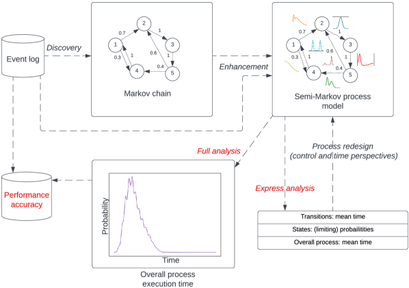
Figure 1. Discovery and performance analysis of stochastic process models.

Process redesign answers “what-if” questions and can be done in two ways: (1) control-flow optimization, which involves changing the structure of the process, i.e., transitions between the states and their probabilities are modified; (2) time optimization: the waiting times of some states are modified. In other words, the process is either structurally reorganized or the time for performing an activity is changed, for example, the time might be reduced by assigning more resources to that task.

Our full analysis (see Subsection 4.2) constructs the full probability distribution of the overall process execution time based on a semi-Markov model, which can be obtained as a result of applying process discovery and enhancement algorithms or at a process redesign step. The semi-Markov model approximates and generalizes the event log, hence, the overall execution time of the model can deviate from the overall execution time observed in the log. To quantify this deviation, performance accuracy of the model can be estimated (Subsection 5.3). This will allow assessment of the quality of the process discovery and enhancement algorithms.

The contributions of this paper are as follows: (1) a method for discovering semi-Markov models from event logs; (2) a new technique (express analysis) to calculate the mean of the overall process execution time using these models; (3) a new method (full analysis) to calculate the distribution of the overall process execution time; and (4) implementation and application of the proposed techniques to real-world event data to estimate the performance accuracy of the discovery algorithms.

2. Preliminaries

In this section, we give basic definitions that will be used to describe the proposed discovery approach.

Information systems record their behavior in the form of event logs represented by sequences of events corresponding to (business) cases. Examples include event logs of web-servers, trouble-ticket, and application management systems. We formally define event logs as follows.

Table 1. A log of an application management system.

	Activity name	Case	Timestamp
$e_{1}$	"Claim"	1	2022-06-17 14:53:03
$e_{2}$	"Claim"	2	2022-06-17 17:33:47
$e_{3}$	"Assign"	1	2022-06-18 12:38:30
$e_{4}$	"Resolve"	2	2022-06-19 09:46:03
$e_{5}$	"Close"	2	2022-06-19 18:57:52
$e_{6}$	"Resolve"	1	2022-06-20 10:37:52
$e_{7}$	"Close"	1	2022-06-20 19:41:23
$e_{8}$	"Resolve"	2	2022-06-21 18:14:51
$e_{9}$	"Assign"	3	2022-06-21 22:56:05
$e_{10}$	"Resolve"	3	2022-06-22 11:09:43
$e_{11}$	"Close"	2	2022-06-22 17:49:46
$e_{12}$	"Close"	3	2022-06-22 22:58:02

Definition 0 (Event log).

Let $E$ be a finite non-empty set of events, $A$ be a set of activity names, $C$ be a finite set of cases, and $T$ be a set of timestamps. An event log is a tuple $L=(E,f_{a},f_{c},f_{t})$, where $f_{a}:E\rightarrow A$ is a function that assigns names to events, $f_{c}:E\rightarrow C$ is a surjective function that maps events to cases, and function $f_{t}:E\rightarrow T$ defines occurrence times for events.

Table 1 presents a fragment of an event log of an information system that processes applications. These can be applications for any kind of services, including government services, publishing, bug tracking, or any other requests managed by an information system.

An application starts with a ”Claim,” which generates a ticket. The ticket is given a unique identifier called a case number, and is ”Assigned” to a team member; then, the request is ”Resolved”; and after that, the ticket is ”Closed”. Alternatively, the ticket can be reopened and the request is resolved once again. Each row in Table 1 represents an event from the finite set of events $E=\{e_{1},e_{2},\dots,e_{12}\}$ and each event is characterized by its name (Activity name column), case or ticket identifier (Case column), and the occurrence time (Timestamp column). For example, event $e_{1}\in E$ is defined as follows: $f_{a}(e_{1})=\text{{"}Claim{"}}$, $f_{c}(e_{1})=1$, and $f_{t}(e_{1})=\text{2022-06-17\leavevmode\nobreak\ 14:53:03}$.

From an event log, we can develop traces. We formally define this below, but loosely these are time-ordered sequences of events grouped by cases.

Definition 0 (Trace of event log).

Let $L=(E,f_{a},f_{c},f_{t})$ be an event log defined over a set of cases $C$. A sequence of events $\delta=\langle e_{1},e_{2},\dots,e_{n}\rangle$, where $e_{1},e_{2},\dots,e_{n}\in E$, is called a trace of $L$ corresponding to case $c$ from $C$ iff it is the longest sequence, such that $\forall i,j$, $1\leq i\leq j\leq n$, it holds that $f_{c}(e_{i})=f_{c}(e_{j})=c$ and $f_{t}(e_{i})\leq f_{t}(e_{j})$.

Note that if two events of the same case have equal timestamps, they can be ordered differently.

Definition 0 (Trace representation of event log).

A set of all traces of log $L$ corresponding to all its cases is a trace representation of $L$, denoted as $\overline{L}$.

Definition 0 (Activity/time traces).

Let $L\nolinebreak=\nolinebreak(E,f_{a},f_{c},f_{t})$ be an event log and $\delta\nolinebreak=\nolinebreak\langle e_{1},e_{2},\dots,e_{n}\rangle\in\overline{L}$ be one of its traces. Then we say that $\delta_{A}\nolinebreak=\nolinebreak\langle f_{a}(e_{1}),f_{a}(e_{2}),\dots,f_{a}(e_{n})\rangle$ is an activity trace and $\delta_{T}=\langle f_{t}(e_{1}),f_{t}(e_{2}),\allowbreak\dots,f_{t}(e_{n})\rangle$ is a time trace corresponding to $\delta$.

Note that activity and time traces have the same length as the original trace.

The event log $L$ presented in Table 1 can be transformed to its trace representation as follows: $\overline{L}=\{\delta^{1},\delta^{2},\delta^{3}\}$, where $\delta^{1}\nolinebreak=\nolinebreak\langle e_{1},e_{3},e_{6},e_{7}\rangle$, $\delta^{2}=\langle e_{2},e_{4},e_{5},e_{8},e_{11}\rangle$, and $\delta^{3}\nolinebreak=\nolinebreak\langle e_{9},e_{10},e_{12}\rangle$. The activity and time traces corresponding to $\delta^{1}$ are $\delta^{1}_{A}\nolinebreak=\nolinebreak\langle\text{{"}Claim{"}},\text{{"}Assign{"}},\text{{"}Resolve{"}},\text{{"}Close{"}}\rangle$ and $\delta^{1}_{T}=\langle t_{1},t_{2},t_{3},t_{4}\rangle$, respectively, where, for example, $t_{1}\nolinebreak=\nolinebreak\scalebox{1.0}{2022-06-17 14:53:03}$ and $t_{2}\nolinebreak=\nolinebreak\scalebox{1.0}{2022-06-18 12:38:30}$.

Now we will introduce common notations used for different types of traces.

Definition 0 (Subtrace, element and trace length).

Consider a trace of elements $\delta=\langle y_{1},y_{2},\dots,y_{n}\rangle$. A subtrace of $\delta$ is a sequence $\langle y_{i},\dots,y_{j}\rangle$, $1\leq i\leq j\leq n$, denoted as $\delta(i,j)$. The $i^{th}$ element of trace $\delta$ is encoded as $\delta(i)$. We denote the length of $\delta$ by $\mathit{len}(\delta)$.

Performance analysis implies that the models discovered from event logs should contain both the control flow and the time perspectives. To capture these two perspectives, we will leverage Markov processes (Ross, 1985).

Definition 0 (Finite-state Markov chain).

Consider a stochastic process $\{X_{n},n=0,1,2,\dots\}$, where random variables $X_{n}$ take on a finite number of possible values (states). We say that $X_{n}=i$ when the stochastic process is in state $i$ at time $n$. We suppose that whenever the stochastic process is in state $i$, there is a fixed probability $p_{i,j}\in[0,1]$ that the next state will be $j$, such that $\sum\limits_{j=1}^{m}p_{i,j}=1$, where $m$ is the number of states. By $\mathbf{P}=(p_{i,j})_{1\leq i,j\leq m}$ we denote the stochastic matrix. We call the stochastic process a (finite-state) Markov chain when $P\{X_{n+1}=j|X_{n}=i,X_{n-1}=i_{n-1},\dots X_{1}=i_{1},X_{0}=i_{0}\}=P\{X_{n+1}=j|X_{n}=i\}=p_{i,j}$, i.e., the choice of the next state depends only on the current state of the process. The transition probability from state $i$ to state $j$ in $k>0$ steps is denoted as $p^{k}_{i,j}=P\{X_{k+l}=j|X_{l}=i\}$.

Markov chains are uniquely defined by their stochastic matrices and can be represented as graphs where nodes correspond to states and direct arcs labeled by $p_{i,j}$ connect states $i$ and $j$ iff $p_{i,j}>0$. Figure 2 presents a Markov chain with the stochastic matrix:

$$\mathbf{P}=\begin{bmatrix}0&1&0\\ 0&0&1\\ 1&0&0\end{bmatrix}.$$

Figure 2. A Markov chain with three states.

Definition 0 (Irreducible Markov chain).

A Markov chain is called irreducible iff every state $i$ can be reached from any other state $j$, i.e., there exists $k$, such that $p^{k}_{i,j}>0$, or there is a path from $i$ to $j$ in its graph representation.

The Markov chain in Figure 2 is irreducible, because all states are reachable from each other.

Definition 0 (State period).

The period $d$ of a state $i$ is the greatest common divisor of the set $W_{i}=\{n:p^{n}_{i,i}>0\}$. A state with period 1 is said to be aperiodic.

If an irreducible Markov chain contains a state of period $d$, then all its states have period $d$, and $d$ is called the period of the Markov chain (Ross, 1985). All the states of the Markov chain in Figure 2 have period 3, because for any $i\in\{1,2,3\}$, $W_{i}=\{3,6,9\dots\}$, and so the Markov chain has period 3.

Definition 0 (Aperiodic Markov chain).

A Markov chain $M$ is called aperiodic iff all its states are aperiodic.

Figure 3. An aperiodic Markov chain.

Figure 3 presents an aperiodic Markov chain, as the greatest common divisor for $W_{1}=W_{2}=\{2,3,4,\dots\}$, as well as for $W_{3}=\{3,5,7,\dots\}$, is 1.

Theorem 10 (Limiting probabilities (Ross, 1985)).

For an irreducible Markov chain with period $d$, limiting probabilities $\pi_{j}=\frac{1}{d}\lim\limits_{n\to\infty}p^{dn}_{i,j}$ exist for all states $j$, and are independent of initial states $i$. The $\pi_{j}$ are the unique non-negative solutions of $\pi_{j}=\sum_{i=1}^{m}\pi_{i}p_{i,j}$ such that $\sum_{j=1}^{m}\pi_{j}=1$, where $m$ is the number of states.

The limiting probability is a long-run chance that the process is in a particular state. For the Markov chain in Figure 3, the system of linear equations has the unique solution: $\pi_{1}=\nicefrac{{2}}{{5}}$, $\pi_{2}=\nicefrac{{2}}{{5}}$, and $\pi_{3}=\nicefrac{{1}}{{5}}$. That is, the process visits state $1$ (or state $2$) twice as often as state $3$.

In the business process management (BPM) and process mining (PM) disciplines, processes are usually considered as a “set of interrelated or interacting activities which transforms inputs into outputs” (ISO 9000:2005, 2005). It is assumed that the process starts by taking inputs as parameters, then a sequence of steps is performed and outputs are produced and the process stops, unlike irreducible Markov process models. Such workflow models with specified start and end nodes were introduced and analyzed in (van der Aalst et al., 2002; Polyvyanyy et al., 2020). To bring the stochastic modelling tools to bear we will define and analyze Markov process flows that have a start and an end state, but such that the end connects to the start to create an irreducible Markov chain.

Definition 0 (Markov process flow).

A Markov chain is called a Markov process flow iff it is irreducible and has a start $s$ and an end $e$ state, such that, $s\neq e$, $p_{e,s}=1$, i.e., state $e$ has only one outgoing transition that leads to state $s$. Markov process flows will be denoted by 3-tuples $(\mathbf{P},s,e)$.

Figure 4. A Markov process flow.

Figure 4 shows a Markov process flow. A Markov process flow is an irreducible Markov chain, and hence, every state $i$ is on a path from $s$ to $e$.

In real-world applications, the time spent in the process’s states can vary. Moreover, the durations of different activities can follow different distribution laws (Rogge-Solti et al., 2014). To cover the time perspective of real-world processes, we will consider process models that assume that the time spent in a particular state is distributed according to an arbitrary distribution law. These are called semi-Markov processes and are formally defined below.

Definition 0 (Semi-Markov process).

Consider a Markov chain with a stochastic matrix $\mathbf{P}=(p_{i,j})_{1\leq i,j\leq m}$. Let $\mathbf{F}=(f_{i,j}(t))_{1\leq i,j\leq m}$, $t\in\mathbb{R}$, be a waiting time matrix and $f_{i,j}(t)$ be probability density functions (PDFs) of the waiting time distribution when moving from state $i$ to state $j$. A semi-Markov process is the Markov chain together with the probability density functions $f_{i,j}(t)$.

Semi-Markov processes are also visualized as graphs and can be characterized as irreducible and aperiodic in respect to their stochastic matrices $\mathbf{P}$ just as for Markov processes.

If the amount of time that the semi-Markov process spends in each state before making a transition is identically 1, then the semi-Markov process is just a Markov chain. If the waiting times are exponentially distributed, then the semi-Markov process is a continuous-time Markov process (Ross, 1985).

Semi-Markov processes are uniquely defined by their stochastic matrix $\mathbf{P}$ and waiting time matrix $\mathbf{F}$, so we encode them as $(\mathbf{P},\mathbf{F})$ pairs. As with Markov processes we can extend semi-Markov processes to our flow model as follows.

Definition 0 (Semi-Markov process flow).

A semi-Markov process $(\mathbf{P},\mathbf{F})$ is called semi-Markov process flow with start $s$ and end $e$ states iff $\mathbf{P}$ encodes a Markov process flow with start and end states $s$ and $e$, respectively.

We will denote semi-Markov process flows as 4-tuples $(\mathbf{P},\mathbf{F},s,e)$.

For the analysis of overall process execution times we will use the notion of a convolution of functions defined below.

Definition 0 (Convolution).

For two PDFs $f(t)$ and $g(t)$ of waiting times, and $t\in\mathbb{R}$, the PDF of the sum of the waiting times will be a convolution $f(t)*g(t)$, such that:

$$f(t)*g(t)=\int\limits_{-\infty}^{\infty}f(\tau)g(t-\tau)d\tau.$$

By $\mathop{\scalebox{1.5}{\raisebox{-0.86108pt}{$\circledast$}}}\limits_{i=1}^{m}f(t)=f(t)*f(t)*\dots*f(t)$ we will denote a multiple $m$-times convolution of a function $f$ with itself .

3. Process Discovery

In this section, we describe how semi-Markov process flows can be discovered from event logs. Algorithm 1 constructs stochastic and waiting time matrices from event logs.

Input: An event log $L$, an order $k$.

Output: A semi-Markov flow $(\mathbf{P},\mathbf{F},s,e)$.

1 $\overline{L}\leftarrow\textrm{ConstructTraceRepresentation}(L)$;

2 $\mathbf{P}\leftarrow\mathbf{0}$ ;

3 // initialize $\mathbf{P}$ with zeros;

4 $\mathbf{F}\leftarrow\mathbf{nil}$ ;

5 // initialize $\mathbf{F}$ with nils;

6 foreach $\delta\in\overline{L}$ do

7       $\delta_{A}\leftarrow\textrm{ConstructActivityTrace}(\delta)$;

8       $\delta_{T}\leftarrow\textrm{ConstructTimeTrace}(\delta)$;

9       /* Connect to start state $s$ */

10       $p_{s,\delta_{A}(1,1)}+=1$;

11       /* Connect states, calculate waiting times and update probability density functions(PDFs) with the waiting times */

12       for $i\leftarrow 1$ to $\mathit{len}(\delta)-1$ do

13             $\Delta_{T}=\delta_{T}(i+1)-\delta_{T}(i)$;

14             if $i<k$ then

15                   $p_{\delta_{A}(1,i),\delta_{A}(1,i+1)}+=1$;

16                   $\textrm{UpdatePDF}(f_{\delta_{A}(1,i),\delta_{A}(1,i+1)},\Delta_{T})$;

17                  

18             else

19                   $p_{\delta_{A}(i-k+1,i),\delta_{A}(i-k+2,i+1)}+=1$;

20                   $\textrm{UpdatePDF}(f_{\delta_{A}(i-k+1,i),\delta_{A}(i-k+2,i+1)},\Delta_{T})$;

21                  

22             end if

23            

24       end for

25      /* Connect to end state $e$ */

26       if $k<\mathit{len}(\delta)$ then

27             $p_{\delta_{A}(\mathit{len}(\delta)-k+1,\mathit{len}(\delta)),e}+=1$;

28            

29       else

30             $p_{\delta_{A}(1,\mathit{len}(\delta)),e}+=1$;

31            

32       end if

33      

34 end foreach

35$p_{e,s}=1$;

36 /* The sum of elements of each row must equal 1 */

37 $\mathbf{P}\leftarrow\textrm{Normalize}(\mathbf{P})$;

38 /* If the waiting time is not defined set it to 0 */

39 for $i,j$ do

40       if $f_{i,j}=nil$ then

41             $\textrm{UpdatePDF}(f_{i,j},0)$;

42            

43      

44 end for

45return $(\mathbf{P},\mathbf{F},s,e)$;

Algorithm 1 SemiMarkovFlowDiscovery

This algorithm takes integer $k>0$ as an additional input parameter that characterizes the “memory” of the process, i.e., the last $k$ events define the current process state.

Similarly to the discovery technique of (van der Aalst et al., 2010b), Algorithm 1 represents each state of the process as a sequence of $k$ event names and connects the states based on the frequencies of events. Another similar discovery method that also considers frequencies of events is Heuristic miner (Weijters et al., 2006), however, it does not analyze performance characteristics of the process.

First, Algorithm 1 constructs a trace representation of the input event log (line 1), initializes the stochastic matrix $\mathbf{P}$ with zero values, assuming that there are no transitions between any of the states (line 2), and labels elements of the waiting time matrix $\mathbf{F}$ as undefined (line 3).

Then, the algorithm traverses through each of the traces analyzing the order of activity names and timestamps and constructing activity and time traces (lines 5–6). Where less than $k$ events are considered (line 12), states are defined as sequences of all activity names seen so far, i.e., $\delta_{A}(1,i)$, where $i$ is the current position, and connected to the next states $\delta_{A}(1,i+1)$. When two states are connected, the corresponding element of the stochastic matrix is increased by 1 (lines 13 and 16). When more than $k$ activity names are considered, states $\delta_{A}(i-k+1,i)$, $\delta_{A}(i-k+2,i+1)$ ($i$ is the current position in the trace) that represented sequences of $k$ last activity names, are connected (line 16). As a result, the stochastic matrix contains weights of transitions (the number of the transitions’ occurrences in the event log) and should be normalized to satisfy the property that the sum of elements of each row is 1 (line 29).

As the algorithm goes through the sequences of activity names, it also analyzes the corresponding time traces. Whenever a new connection between the states is added, the time difference between the occurrences of the event in the position $i+1$ and the event in the position $i$ is calculated (line 11). We assume that the waiting time for a transition is the difference in start times of the current and the next event. After the waiting time is calculated, the corresponding PDF is updated taking into account this new time value (lines 14–17). There exist various approximation methods for PDFs (Rogge-Solti et al., 2014; Barron and Sheu, 1991; Wilson and Wragg, 1972), however, here we use a performance analysis focused on the approximation of PDFs using Gaussian Mixture Models (GMMs), as this allows us to model arbitrary waiting times (refer to Subsection 5.2).

The start state $s$ and end state $e$ are connected to the states corresponding to the first (line 8) and the last events (lines 21–25) in the log. These connections are proportional to the frequencies of the first and the last events. The backward transition from $e$ to $s$ is added in line 27. Note that the waiting time is not defined for the transitions from and to the start and end states, and in these cases, we set their waiting times to zero (lines 30–34). By construction, each state lies on a path from $s$ to $e$, and thus this backward transition creates an irreducible semi-Markov process.

Figure 5 visualizes a stochastic matrix $\mathbf{P}$ with designated states $s$ and $e$ discovered by Algorithm 1 from the event log $L$ (see Section 2) when the parameter $k$ is set to 1.

Figure 5. A Markov process flow discovered from event log $L$ with $k$ set to 1.

Increasing the parameter $k$ will lead to process models in which the next state is defined by the last $k$ events in the trace. Such models are known as Markov processes of order $k$ (Ching et al., 2004).

Figure 6 presents a process discovered by Algorithm 1 for $k$=2, when the maximum length of the sequences that define the next state is 2.

Figure 6. A Markov process flow discovered from $L$ with $k$ set to 2.

4. Performance Analysis

This section presents two types of performance analysis. First we present express analysis for the calculation of the mean of the process execution time; this type of analysis also provides additional information on the contribution of each of the process states. Second we present full analysis that calculates a PDF for the overall process execution time.

4.1. Express analysis. Deriving Mean of Process Execution Time

In this subsection, we propose new formulas to estimate the overall process execution time. These results provide analytical solutions that also assess the contribution of process states to the overall process execution time and are based on their limiting probabilities. These results can be further used in a what-if analysis.

First, we prove specific properties of limiting probabilities for Markov process flows that will be used later in this subsection. Let $\mathbf{P}=(p_{i,j})$ be a stochastic matrix of a Markov process flow $(\mathbf{P},s,e)$. Then, by $\widehat{\mathbf{P}}=(\widehat{p}_{i,j})$ we will denote a matrix, such that, $\widehat{p}_{i,j}=0$, if $i=e,j=s$, and $\widehat{p}_{i,j}=p_{i,j}$, otherwise. This matrix assumes that there is no edge from $e$ to $s$. By $\widehat{p}^{\text{ }l}_{i,j}$ we denote a transition probability in $l$ steps from $i$ to $j$ in this Markov chain.

Lemma 0 (Properties of limiting probabilities of Markov process flows).

Let $(\mathbf{P},s,e)$ be a Markov process flow and $\pi_{r}$ be a limiting probability for state $r$. Then $\pi_{r}=\pi_{s}\sum\limits_{l=0}^{\infty}\widehat{p}_{s,r}^{\text{ }l}$, i.e., the limiting probability of state $r$ can be defined as the limiting probability of the start state multiplied by the sum of all transition probabilities from $s$ to $r$ without transiting through $(e,s)$ edge.

Proof.

By Theorem 10, $\pi_{r}=\frac{1}{d}\lim\limits_{n\to\infty}p_{s,r}^{dn}$, and this limit can be represented as:

$$\pi_{r}=\frac{1}{d}\lim\limits_{{\begin{subarray}{c}n_{1}\to\infty\\ n_{2}\to\infty\end{subarray}}}p_{s,s}^{dn_{1}}\sum\limits_{l=0}^{n_{2}}\text{ }\widehat{p}_{s,r}^{\text{ }l}\,,$$

because if a path from $s$ to $r$ contains $e$, state $s$ will be visited once again, and, hence, we consider all the possibilities of reaching $r$ from $s$ in $dn_{1}+n_{2}$ steps in total. The limit as $n_{1},n_{2}\to\infty$ equals $\pi_{s}\sum\limits_{l=0}^{\infty}\widehat{p}_{s,r}^{\text{ }l}$, and, hence $\pi_{r}=\pi_{s}\sum\limits_{l=0}^{\infty}\widehat{p}_{s,r}^{\text{ }l}$. ∎

Lemma 1 provides results that can be used for the calculation of the mean of the process execution time.

Theorem 2 (Mean of process execution times).

Let $(\mathbf{P},\mathbf{F},s,e)$ be a semi-Markov process flow. Then, mean $\mu$ of hitting time for state $e$ when the process has started in state $s$ (the mean of the overall execution time) can be calculated as follows:

(1) $$\mu=\frac{1}{\pi_{s}}\sum\limits_{{\begin{subarray}{c}i=1,\\ i\neq e\end{subarray}}}^{m}\pi_{i}\mu_{i}\,,$$

where $\pi_{s}$ is the limiting probability for the start state $s$, $\pi_{i}$ and $\mu_{i}$ are the limiting probability and the mean time, respectively, for the state $i$, and $i$ iterates over all $m$ states except end state $e$.

Proof.

Consider a matrix $\mathbf{Q}=(q_{i,j}(t))_{1\leq i,j\leq m}$, $t\in\mathbb{R}$, such that $q_{i,j}(t)=\widehat{p}_{i,j}f_{i,j}(t)$, where $\widehat{p}_{i,j}$ is the element of $\mathbf{\widehat{P}}$ (the probability matrix corresponding to the original matrix $\mathbf{P}$, but with no edges from the state $e$). We define matrix $\mathbf{Q}^{n}$ as follows: $\mathbf{Q}^{n}=\mathbf{Q}^{n-1}*\mathbf{Q}$, where $n\geq 1$, $\mathbf{Q}^{1}=\mathbf{Q}$. Multiplication for matrices of functions we define in such a way that $C=A*B$, when $c_{i,j}(t)=\sum\limits_{r=1}^{m}a_{i,r}(t)*b_{r,j}(t)$, where $*$ is the convolution operation. By $q_{i,j}^{n}(t)$ we will denote the $i,j$-element of the matrix $\mathbf{Q}^{n}$.

As can be inferred from (Pyke, 1961), the overall process execution time (hitting state $e$ assuming that the process has started in state $s$) is $f(t)=\sum\limits_{n=1}^{\infty}q_{s,e}^{n}(t)$, i.e., the weighted time of hitting $e$ in 1 step, 2 steps, etc. Hence, the mean of process execution time can be calculated as:

$$\mu[\sum\limits_{n=1}^{\infty}q_{s,e}^{n}(t)]=\sum\limits_{n=1}^{\infty}\mu[q_{s,e}^{n}(t)]= \mu[q_{s,e}^{1}(t)]+\mu[q_{s,e}^{2}(t)]+\mu[q_{s,e}^{3}(t)]+\dots=\mu[p_{s,e}f_{s,e}(t)]+$$

$$\mu[\sum\limits_{{\begin{subarray}{c}i=1\\ i\neq e\end{subarray}}}^{m}(p_{s,i}f_{s,i}(t)*p_{i,e}f_{i,e}(t))]+\mu[\sum\limits_{{\begin{subarray}{c}i,j=1\\ i,j\neq e\end{subarray}}}^{m}(p_{s,i}f_{s,i}(t)*p_{i,j}f_{i,j}(t)*p_{j,e}f_{j,e})]+\dots\,.$$

Since $\mu[f(t)*g(t)]=\mu[f(t)]+\mu[g(t)]$, this expression can be rewritten as:

$$p_{s,e}(\mu[f_{s,e}(t)])+\sum\limits_{{\begin{subarray}{c}i=1\\ i\neq e\end{subarray}}}^{m}p_{s,i}p_{i,e}(\mu[f_{s,i}(t)]+\mu[f_{i,e}(t)])+\sum\limits_{{\begin{subarray}{c}i,j=1\\ i,j\neq e\end{subarray}}}^{m}p_{s,i}p_{i,j}p_{j,e}(\mu[f_{s,i}(t)]+\mu[f_{i,j}(t)]+\mu[f_{j,e}])+\dots\,.$$

After rearrangement of terms we get:

$$\sum\limits_{{\begin{subarray}{c}i=1\\ i\neq e\end{subarray}}}^{m}\sum\limits_{l=0}^{\infty}\widehat{p}_{s,i}^{\text{ }l}\sum\limits_{l=0}^{\infty}\widehat{p}_{i,e}^{\text{ }l}\mu[\sum\limits_{j=1}^{m}p_{i,j}f_{i,j}(t)]\,.$$

By Lemma 1 and because $\sum\limits_{l=0}^{\infty}\widehat{p}_{i,e}^{\text{ }l}=1$ (the probability of eventually hitting state $e$), the expression can be represented as:

$$\sum\limits_{{\begin{subarray}{c}i=1\\ i\neq e\end{subarray}}}^{m}\frac{\pi_{i}}{\pi_{s}}\mu[\sum\limits_{j=1}^{m}p_{i,j}f_{i,j}(t)]=\frac{1}{\pi_{s}}\sum\limits_{{\begin{subarray}{c}i=1\\ i\neq e\end{subarray}}}^{m}\pi_{i}\mu_{i}\,,$$

where $\mu_{i}$ is the mean time for state $i$. ∎

Theorem 2 provides results that can be used in practice to estimate the overall process execution time based on the time distributions for each of the states. This method does not rely on any particular PDF (probability density function) approximation, allowing estimation of the mean time using simple formulas for a finite number of observations.

Let $[\Delta_{T_{1}},\Delta_{T_{2}},\dots,\Delta_{T_{n}}]$ be a multiset of time durations when moving from state $i$ to state $j$, extracted from the event log (Algorithm 1). The $\mathit{UpdatePDF}$ function can be implemented to recalculate the mean values $\mu_{i}=\sum\limits_{j=1}^{m}p_{i,j}\frac{\sum\limits_{r=1}^{n}\Delta_{T_{r}}}{n}$ each time new durations are added. After that, limiting probabilities are retrieved as a solution of linear equations (Theorem 10) and a mean value $\mu=\frac{1}{\pi_{s}}\sum\limits_{{\begin{subarray}{c}i=1\\ i\neq e\end{subarray}}}^{m}\pi_{i}\mu_{i}$ of the overall execution time is calculated (Theorem 2).

This general approach can be applied when PDFs are known or inferred using an approximation algorithm. It can also be applied for a what-if analysis, allowing one to estimate the impact of each of the states on the overall process execution time.

Consider an example of event log (Table 1) and a corresponding Markov process flow discovered from this event log with $k$ set to 1 (Figure 5). The mean waiting times for the states extracted from the event log are: $\mu_{1}$=1d : 6h : 58m : 52s, $\mu_{2}$=13h : 24m : 39s, $\mu_{3}$=11h : 49m : 15s, $\mu_{4}$=1d : 5h : 6m : 30s, and $\mu_{s}=\mu_{e}=0$. The limiting probabilities are the following: $\pi_{1}=\nicefrac{{1}}{{9}}$, $\pi_{2}=\nicefrac{{2}}{{9}}$, $\pi_{3}=\nicefrac{{2}}{{9}}$, $\pi_{4}=\nicefrac{{1}}{{9}}$, and $\pi_{s}=\pi_{e}=\nicefrac{{1}}{{6}}$. According to Equation 1, the mean of the overall process execution time is 3d : 1h : 42m : 5s.

Now a what-if analysis can be run, and the process can be optimized in two ways: (1) reducing the waiting time for some of the states (reducing $\mu_{i}$ values); (2) reorganizing the structure of the process (changing $\pi_{i}$ values).

Firstly, to optimize the process we may try to reduce waiting times for the states with the highest impact (highest limiting probabilities), these are states $2$ and $3$, or highest waiting times, these are states $1$ and $4$. Reducing waiting times for states $1$ and $4$ means we reduce the time before the event labeled by the activity name "Resolve" occurs. This can be achieved by assigning more resources (employees) who resolve the requests. Suppose that the waiting times for states $1$ and $4$ were halved, and the new mean times are $\mu^{\prime}_{1}$=15h : 29m : 26s and $\mu^{\prime}_{4}$=14h : 33m : 15s, respectively. Then, according to Equation 1, the new mean of the overall process execution time is 2d : 5h : 40m : 19s, which is considerable improvement comparing to the original time 3d : 1h : 42m : 5s.

Another way to optimize the process is to modify the limiting probabilities changing the stochastic matrix, and hence, the structure of the process. A Markov process flow (Figure 5) assumes that in half of the cases a ticket that was claimed by an employee can be reassigned (or approved) later. This can lead to potential delays. It may be feasible to allow most of the employees to start working on applications they have already requested without further approval. An optimized Markov process flow in which only 10% of ticket claims are to be reassigned (approved) is presented in Figure 7. In this case the limiting probabilities will be: $\pi^{\prime}_{1}=\nicefrac{{10}}{{86}}$, $\pi^{\prime}_{2}=\nicefrac{{20}}{{86}}$, $\pi^{\prime}_{3}=\nicefrac{{20}}{{86}}$, $\pi^{\prime}_{4}=\nicefrac{{6}}{{86}}$, and $\pi^{\prime}_{s}=\pi^{\prime}_{e}=\nicefrac{{15}}{{86}}$, and, according to Equation 1, the mean of the overall process execution time is: 2d : 17h : 56m : 23s, which is less than the mean of the overall time (3d : 1h : 42m : 5s) for the original process.

Figure 7. An optimized Markov process flow corresponding to the original process model presented in Figure 5. In contrast to Figure 5, transitions between states $1^{\prime}$ and $4^{\prime}$, $1^{\prime}$ and $2^{\prime}$, have 0.1, 0.9 probabilities, respectively.

Although the model discovered by the proposed algorithm allows for more behavior in terms of sequences of events and their execution times, the mean time of one process run for the discovered model and the mean trace time for the corresponding event log are the same.

Theorem 3 (Log and model mean times).

Let $L$ be an event log and $M=(\mathbf{P},\mathbf{F},s,e)$ be a semi-Markov process flow discovered from this log by Algorithm 1, with an arbitrary order $k$ set as a parameter. Then, the mean process execution times for the log and the model are the same, i.e., $\mu_{M}=\mu_{L}$, where $\mu_{M}$ is the mean $e$ hitting time and $\mu_{L}$ is the mean duration of a trace for the event log $L$.

Proof.

The mean trace duration for event log $L$ can be represented as the sum of durations of all traces divided by the number of traces, i.e., $\mu_{L}=\sum\limits_{\langle e_{1}\dots e_{n}\rangle\in\overline{L}}(f_{t}(e_{n})-f_{t}(e_{1}))/|\overline{L}|$, where $\overline{L}$ is the trace representation of $L$. That equals to the sum of durations of all events divided by the number of traces. Formally, the mean trace duration is defined as: $\mu_{L}=\sum\limits_{\langle e_{1}\dots e_{n}\rangle\in\overline{L}}\left[\sum\limits_{j=1}^{n-1}(f_{t}(e_{j+1})-f_{t}(e_{j}))\right]/|\overline{L}|$. For each event $e_{j}$ from $L$, consider the activity name sequence $\langle f_{a}(e_{j-k+1}),f_{a}(e_{j-k+2}),\dots,f_{a}(e_{j})\rangle$ of length $k$ and rename it as $\langle a_{1},a_{2},\dots,a_{k}\rangle$. This sequence corresponds to a state in $M$ and can occur in $L$ multiple times. Let $\#\langle a_{1},a_{2},\dots,a_{k}\rangle$ be the number of occurrences of $\langle a_{1},a_{2},\dots,a_{k}\rangle$ in $L$ and let $\mu_{j}$ be the mean time spent by $M$ in the state $\langle a_{1},a_{2},\dots,a_{k}\rangle$. Because $\mu_{j}$ is the sum of the execution times over all events $e_{j}$, such that $f_{a}(e_{j-k+1})=a_{1},f_{a}(e_{j-k+2})=a_{2},\dots,f_{a}(e_{j})=a_{k}$, divided by the number of occurrences of $\#\langle a_{1},a_{2},\dots,a_{k}\rangle$, the trace mean duration can be defined as $\sum\limits_{\langle a_{1},a_{2},\dots,a_{k}\rangle\text{ in }L}\#\langle a_{1},a_{2},\dots,a_{k}\rangle\mu_{j}/|\overline{L}|$. The number of occurrences of the sequence $\langle a_{1},a_{2},\dots,a_{k}\rangle$ equals to the weighted sum of the number of occurrences of preceding sequences, i.e., $\#\langle a_{1},a_{2},\dots,a_{k}\rangle=\sum\limits_{j=1}^{m}p_{j,i}\#\langle a^{\prime}_{0},a_{1},a_{2},\dots,a_{k-1}\rangle$, proportionally to the frequencies of transitions which connect the corresponding states (Algorithm 1). Hence, the occurrences of $k$-length sequences satisfy the system equations: $\pi_{i}=\sum\limits_{j=1}^{m}p_{j,i}\pi_{j}$ (from Theorem 10), and are proportional to the corresponding limiting probabilities of $M$, i.e. $\#\langle a_{1},a_{2},\dots,a_{k}\rangle=c\pi_{i}$, where $c$ is a coefficient. Similarly, the number of traces $|\overline{L}|$ can be calculated as the number of occurrences of the last events, and it is equal to $c\pi_{e}=c\pi_{s}$. Thus, $\mu_{L}=\sum\limits_{j=1}^{m^{\prime}}\frac{c\pi_{j}\mu_{j}}{c\pi_{s}}=\frac{1}{\pi_{s}}\sum\limits_{j=1}^{m^{\prime}}\pi_{j}\mu_{j}$, where $m^{\prime}$ is the total number of distinct activity name sequences of the length $k$ in $L$. Since $\mu_{s}=\mu_{e}=0$, $\mu_{L}=\frac{1}{\pi_{s}}\sum\limits_{{\begin{subarray}{c}j=1\\ j\neq e\end{subarray}}}^{m}\pi_{j}\mu_{j}$, that is $\mu_{M}$ by Theorem 2. ∎

Note that the mean time for the event log (Table 1) is the same as for the model discovered from this event log (Figure 5), and it equals 3d : 1h : 42m : 5s.

4.2. Full Analysis Of The Process Execution Time

This section presents a method that calculates a PDF for the overall process execution time using a so-called reduction technique. This reduction technique is based on the algorithm that builds regular expressions from finite state automata models (Hopcroft et al., 2007). Conversion of semi-Markov models to regular expressions using this type of algorithm was first discussed in (Csenki, 2008). However, it was not implemented and was not applied to real-world data. In this work, we provide, implement and test a complete reduction algorithm for the construction of PDFs for the overall execution time of semi-Markov process flows.

Consider a fragment of a semi-Markov process flow that is represented by a graph, where nodes correspond to the process states and edges are labeled by transition probabilities and PDFs of waiting times (8(a)).

(a) A fragment of a semi-Markov process flow.

(b) The semi-Markov process flow after reduction of state $2$.

Figure 8. Eliminating state from a semi-Markov process flow.

The reduction algorithm removes all the states (except start and end states) adding new transitions corresponding to the removed paths. 8(a) presents a fragment of a semi-Markov process flow before the reduction. The corresponding fragment after the elimination of state $2$ is shown in 8(b). Once state $2$ is removed, all the states that were connected via this state, will be connected directly. Corresponding transitions will be labeled with new probabilities and PDFs. For example, the new transition that links states $1$ and $4$ is labeled by $p_{1,2}\frac{p_{2,4}}{p_{2,4}+p_{2,5}}$ – the probability of transitioning from state $1$ to state $4$ via state $2$ in the original semi-Markov model. The new PDF for the transition time from $1$ to $4$ via state $2$ is defined as $f_{1,2}(t)\!*\!\overset{\scaleobj{0.9}{\leftturn}}{f_{2}}(t)\!*\!f_{2,4}(t))$, where $\overset{\scaleobj{0.9}{\leftturn}}{f_{2}}(t)=(1-p_{2,2})\left(f^{0}(t)+\sum\limits_{\mathcal{s}=1}^{\infty}p^{\mathcal{s}}_{2,2}\mathop{\scalebox{1.5}{\raisebox{-0.86108pt}{$\circledast$}}}\limits_{r=1}^{\mathcal{s}}f_{2,2}(t)\right)$ is a PDF for the looping time in state $2$, and

$$f^{0}(t)=\begin{cases}1,&\text{if $t=0$}.\\ 0,&\text{otherwise}.\end{cases}.$$

Note that, states $1$ and $4$ are not necessarily distinct and the elimination of state $2$ can lead to self-loops.

The case of merging multiple transitions leading to one state should be included to the general case (Figure 8), but for the sake of clarity, we consider this case separately. 9(a) presents an initial fragment of a Markov process flow. The result of state $2$ reduction, such that transitions between nodes $1$ and $3$ are merged is presented in 9(b). The probability for the new transition between states $1$ and $3$ will be defined as $p_{1,2}+p_{1,3}$ and the corresponding PDF will be a weighted sum of PDFs of waiting times for moving from state $1$ to $3$ directly and via state $2$.

(a) A fragment of a Markov process flow with an additional transition.

(b) The Markov process flow without state $2$.

Figure 9. Reduction of the Markov process flow. Multiple transitions case.

This approach allows us to reduce the original Markov process flow iteratively so that only states $s$ and $e$ remain. The transition between these two states will be marked by a pair $(1,f_{\mathit{total}}(t))$, where $f_{\mathit{total}}(t)$ is the PDF for $e$ hitting time.

The next subsection discusses the approach implemented in this paper for the representation and manipulation of PDFs of waiting times using Gaussian Mixture Models.

4.3. Representation of Probability Density Functions

For the express analysis no specific representation of waiting times is required, because we are only interested in the mean of waiting times; but for the full analysis, a PDF of the overall process execution time needs to be inferred from the event data.

Transitions in the discovered semi-Markov processes are annotated with PDFs of waiting times. The representation of these PDFs plays a crucial role in the further analysis and inference of the overall process execution time. Algorithm 1 collects waiting times for each pair of states $i$ and $j$ and updates the PDF $f_{i,j}(t)$ accordingly.

As will be shown later, waiting times in real-world event data can follow a whole a range of distributions, including multi-modal distributions. Gaussian Mixture Models (GMMs) are ideal to encompass multi-modal data. The PDFs of GMMs are of the form: $f(t)=\sum\limits_{i=1}^{\ell}q_{i}g_{i}(t)\text{, where }\sum\limits_{i=1}^{\ell}q_{i}=1\text{, and }$

$$g_{i}(t)=\frac{1}{\sigma_{i}\sqrt{2\pi}}e^{-\frac{1}{2}\left(\frac{t-\mu_{i}}{\sigma_{i}}\right)^{2}},$$

is a PDF of a Gaussian distribution with mean $\mu_{i}$ and variance $\sigma^{2}_{i}$.

A key advantage of GMMs is that the convolution of two Gaussians $g(t)$ and $h(t)$ is a Gaussian $g(t)*h(t)$, such that $\mu_{g*h}=\mu_{g}+\mu_{h}$ and $\sigma^{2}_{g*h}=\sigma^{2}_{g}+\sigma^{2}_{h}$, i.e., the mean and variance are sums of means and variances, respectively. This simplifies the calculation of convolution for two GMMs, e.g., according to the distributive property of convolution: $f(t)=(p_{1}g_{1}(t)+p_{2}g_{2}(t))*(p_{3}h_{1}(t)+p_{4}h_{2}(t))=p_{1}p_{3}(g_{1}(t)*h_{1}(t))+p_{2}p_{3}(g_{2}(t)*h_{1}(t))+p_{1}p_{4}(g_{1}(t)*h_{2}(t))+p_{2}p_{4}(g_{2}(t)*h_{2}(t))$.

As the time distributions are represented only by mean and variance values, this approach allows us to perform running computations for large-scale event data.

There is one minor caveat — Gaussian distributions have infinite support and as waiting times are non-negative we need, at some point, to truncate this representation. We discuss our approach to this truncation in our case study, described below.

5. Case Studies

In this section, we apply performance analysis techniques to event data from a real-world incident management system’s event log (BPI’13 incidents (Steeman, 2013b)) as a running example. The case study also addresses some practical components of the algorithm such as the choice of the model order $k$, and approaches for practical issues such as truncation.

Firstly, we leverage the express analysis technique to estimate the process mean time and run a what-if analysis (Subsection 5.1). We then explore how different types of time distributions in event data can be approximated using GMMs (Subsection 5.2), and after that, we apply the full performance analysis technique to real-world event data and analyze its accuracy (Subsection 5.3).

The proposed methods were implemented in Python using the PM4PY library (Berti et al., 2019) and are available at:
https://github.com/akalenkova/TimeDistributions.

5.1. Applying Express Analysis to Real-World Event Data

An incident management system of Volvo IT Belgium recorded the history of the production incident processes in the form of an event log (Steeman, 2013b). This event log contains 7,554 traces, 65,533 events, and 4 event names (”Accepted”, ”Queued”, ”Completed”, or ”Unmatched”). Each incident record was processed by a management team and the results were recorded in the log. Figure 10 shows a graphical representation of the Markov process flow discovered by Algorithm 1 with the order $k$ set to 1.

Figure 10. A Markov process flow (where $s$ is a start state and $e$ is an end state) discovered from the log of an incident management system with k=1, i.e., each state corresponds to a preceding sequence of activities of length 1.

Most commonly, once the process has started, the incident description is accepted, and then it is either accepted again (for example, by a different employee) or the management procedure is completed. Alternatively, if there are not enough resources to process the request, it is queued. In rare cases, when the status of the request is unknown, the incident description is labeled as ”Unmatched” and is considered again.

Once the model is discovered, a what-if analysis can be applied. By Theorem 2, the mean time of the process is $\mu=\frac{1}{\pi_{s}}\sum\limits_{{\begin{subarray}{c}i=1\\ i\neq e\end{subarray}}}^{m}\pi_{i}\mu_{i}$, where $\pi_{i}$ and $\mu_{i}$ are the limiting probabilities and mean waiting times, respectively. This process is represented by the following limiting probabilities and times: $[0.09367,0.49748,0.14316,0.17196,0.00006,0.09367]$, $[\text{0d 0h 0m 0s},\allowbreak\text{1d 5h 8m 9s},\text{1d 2h 9m 35s},\text{2d 3h 51m 27s},\allowbreak\text{0d 0h 11m 10s},\text{0d 0h 0m 0s}]$ retrieved for the vector of process states: $[s,\langle\text{{"}Accepted{"}}\rangle,\langle\text{{"}Queued{"}}\rangle,\langle\text{{"}Completed{"}}\rangle,\allowbreak\langle\text{{"}Unmatched{"}}\rangle,\allowbreak e]$.

As can be calculated using the formula $\mu=\frac{1}{\pi_{s}}\sum\limits_{{\begin{subarray}{c}i=1,i\neq e\end{subarray}}}^{m}\pi_{i}\mu_{i}$, the mean process execution time is 12d 1h 54m 15s. The state with the largest value of $\pi_{i}\mu_{i}$ has the greatest impact on the overall performance of the process. In this case, this state is $\langle\text{{"}Accepted{"}}\rangle$. Although the state with the greatest mean time is $\langle\text{{"}Completed{"}}\rangle$, the state $\langle\text{{"}Accepted{"}}\rangle$ is the most time-consuming because of its limiting probability i.e., it occurs more often than other states. The waiting time in the state $\langle\text{{"}Accepted{"}}\rangle$ corresponds to the actual incident management; if more staff were assigned to this process step, it would reduce the overall mean time. If the mean time for the $\langle\text{{"}Accepted{"}}\rangle$ state were decreased by a factor of two, the average time of the entire process (calculated using the formula for the mean value) would be 8d 20h 32m 19s.

Another way to improve the performance characteristics of the process is to reorganize its structure and adjust the transition probabilities. This will change the limiting probabilities, and hence, the overall execution time.

5.2. Deriving Continuous Execution Times From Event Logs

In this subsection, we demonstrate how PDFs of waiting times between the states can be derived from event data. As proposed in Subsection 4.3, PDFs will be represented in a form of GMMs.

Once waiting times for a pair of process states have been collected by Algorithm 1, the corresponding time distribution is derived in the form of a GMM. We do so by first approximating the data using a Kernel Density Estimator (KDE) with a Gaussian kernel to build a smooth and general representation of the PDF.

We then fit a GMM to the KDE representation by optimising the fit of $\sum\limits_{i=1}^{\ell}q_{i}g_{i}(t)$, where $\sum\limits_{i=1}^{\ell}q_{i}=1$ and each $g_{i}(t)$ is a Gaussian with a mean $\mu_{i}$ and variance $\sigma^{2}_{i}$. The result is a set of optimal fitting parameters: $\ell$, $q_{i}$, $\mu_{i}$, and $\sigma^{2}_{i}$, for $1\leq i\leq\ell$.

Figure 11 presents histograms of two time distributions and their continuous KDE and GMM approximations: (1) for the self-loop transition of the state $\langle\text{{"}Completed{"}}\rangle$ (Figure 11(a)), and, (2) for the transition between the states $\langle\text{{"}Queued{"}}\rangle$ and $\langle\text{{"}Completed{"}}\rangle$. This example demonstrates that durations of events in real-world can be far from exponentially distributed. Hence, regular Markov processes are not always applicable. Models such as semi-Markov processes are needed to capture such distributions with any degree of accuracy.

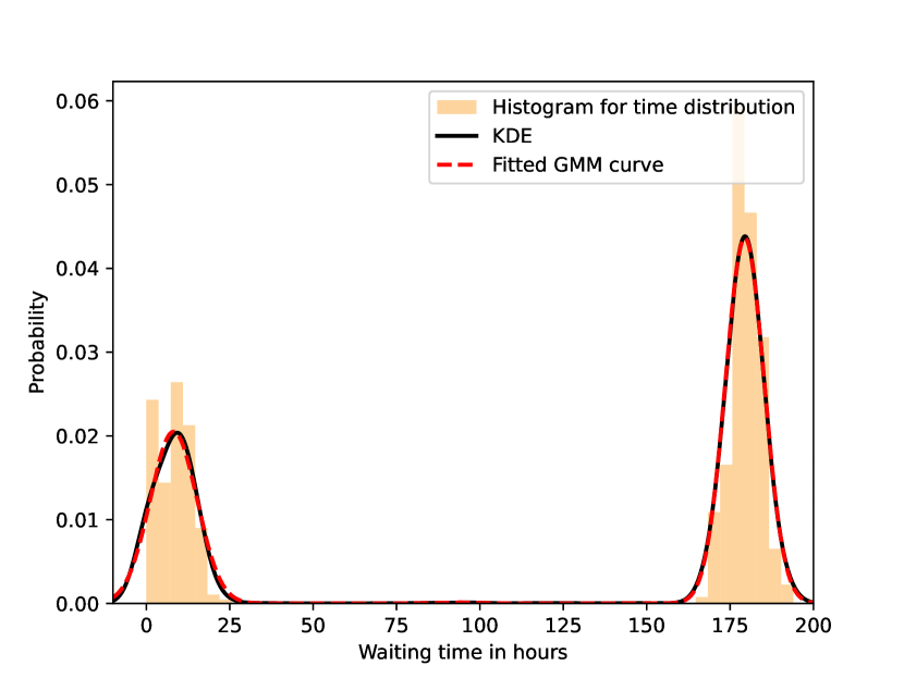
(a) PDFs $f_{3,3}(t)$ of the waiting times for the transition $(3,3)$, i.e., the self-loop transition of the $\langle\text{{"}Completed{"}}\rangle$ state.

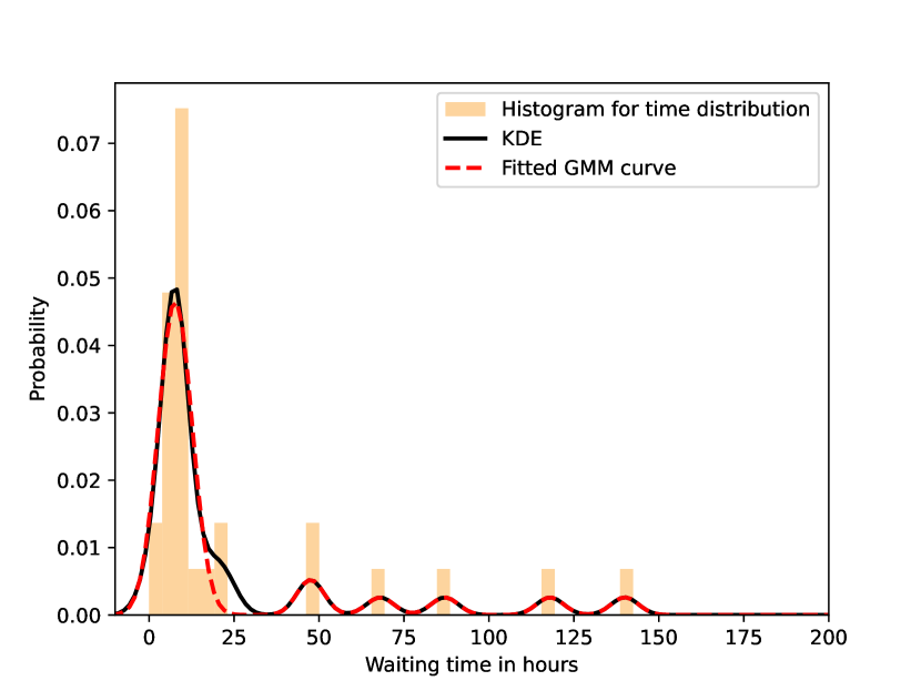
(b) PDFs $f_{2,3}(t)$ of the waiting times for the transition $(2,3)$, i.e., the transition between states $\langle\text{{"}Queued{"}}\rangle$ and $\langle\text{{"}Completed{"}}\rangle$.

Figure 11. PDFs of the waiting times for the transitions of the semi-Markov process flow presented in Figure 10. Discrete PDFs in the form of histograms with 200 bins are presented in light orange. KDE approximations (with Gaussian kernel and bandwidth of 4) and fitted GMMs are black and dashed red, respectively.

Note that a GMM permits negative execution times. However, it is easy to see that for the GMM that fits to the data shown in Figure 11 this is an almost trivial issue, as is usually the case. We will also demonstrate, in the next subsection, that even with the possibility of negative times, accurate performance models can be derived.

Also in Figure 11 we see how the KDE process smooths the original data. This is a deliberate form of regularization used to increase the generalizability of results. That is, smoothing helps prevent overfitting to aspects of a particular trace, making conclusions drawn from the process more robust. The GMM model fitting, for instance, is more robust when applied to KDE results, than if applied to raw data. However, rather than measuring the quality of this fit, we will show in our results the quality of the inferences obtained from this process, which is a more reliable measure of the process than simplistic measures of the quality of fits along the way.

5.3. Relating Discovered and Observed Process Execution Times

In this subsection, we apply the proposed full analysis approach to real-world event data including the dataset described above and also including 2 additional datasets. The three logs are from:

• the earlier discussed incident management system of Volvo IT Belgium (BPI’13 incidents (Steeman, 2013b) event log); and

• a university travel expense claim system (Domestic Declarations – DD’20 (van Dongen, 2020a) and Request For Payment –RFP’20 (van Dongen, 2020d) event logs).

Table 4 presents the number of traces and events, as well as the number of event names in these event logs. The median trace length for all the event logs is 5.

Table 2. Characteristics of the real-world event logs.

Event log	# Traces	# Events	# Event names
BPI'13 incidents	7,554	65,533	4
DD'20	10,500	56,437	17
RFP'20	6,886	36,796	19

For the analyzed datasets, all activity durations were rounded and estimated in hours, and then corresponding semi-Markov models of order from 1 to 5 were discovered. To estimate the discovery time and the overall GMMs fitting time, we ran 5 experiments for each event log and each order $k$. Table 3 shows the order, size (number of states and transitions), mean and 95% CIs (confidence intervals) for the discovery and GMMs fitting times in seconds . As the results suggest, the discovery algorithm is computationally negligible, but it takes more time to find all GMMs to annotate transitions of the discovered models. Usually, the larger the discovered model is (the more transitions it contains), the more time is needed to build all GMMs. However, in the case of RFP’20 event log, durations of transitions of higher-order models can be approximated faster, this can be explained by the fact that the optimizing fitting algorithm can converge differently depending on the input data.

Table 3. Order, size, discovery and overall GMMs fitting times for models constructed from real-world event data.

Event log	Order $k$	# States	# Transitions	Disc. time (in sec.)	GMMs fit. time (in sec.)
	1	6	17	0.63 $\pm$0.07	11.47$\pm$0.90
BPI'13	2	16	47	0.67$\pm$0.12	13.57$\pm$1.04
incidents	3	42	105	0.78$\pm$0.13	18.52$\pm$1.45
	4	91	219	0.68$\pm$0.05	43.75$\pm$3.33
	5	191	432	0.75$\pm$0.05	127.18$\pm$1.65
	1	19	48	0.47$\pm$0.00	27.09$\pm$1.35
	2	43	90	0.48$\pm$0.01	434.47$\pm$11.37
DD'20	3	75	139	0.59$\pm$0.05	470.78$\pm$3.64
	4	118	197	0.63$\pm$0.05	535.37$\pm$11.34
	5	168	256	0.60$\pm$0.04	538.41$\pm$7.70
	1	21	57	0.35$\pm$0.01	53.52$\bf\pm$0.88
	2	48	99	0.43$\pm$0.08	78.54$\pm$1.34
RFP'20	3	81	151	0.41$\pm$0.04	57.18$\pm$0.78
	4	124	204	0.39$\pm$0.03	34.17$\pm$0.44
	5	169	255	0.38$\pm$0.01	30.02$\pm$0.32

The reduction of states is another computationally expensive problem. To lower its time complexity, we pruned the number of Gaussians in GMMs using a probability threshold. After each state reduction, all the Gaussians in any new GMM with weight coefficients less than this threshold were merged into one Gaussian with a mean and variance corresponding to the mean and variance of the weighted sum of the merged Gaussians. Also, only self-loop repetitions with the probability $(1-p)p^{\mathcal{s^{\prime}}}$, where $p$ is the probability of a self-loop and $\mathcal{s^{\prime}}$ is the number of self-loop repetitions, larger than the threshold were considered. This optimization allowed us to compute an upper bound for the time computational complexity of the reduction algorithm to be $O(n^{3}\cdot\ell^{2}+n\cdot\mathcal{s}\cdot\ell^{2})$, where $n$ is the number of states in the model, $\ell$ is the maximum number of Gaussians in a GMM, and $\mathcal{s}$ is the maximum number of self-loop repetitions.

To relate the observed and discovered process execution times we plotted the time distributions for the event logs and semi-Markov models discovered from these event logs. Figure 12 shows the overall time distributions for two of the event logs compared to the estimated times for semi-Markov models of order $k$ from 1 to 5 discovered from these event logs with the threshold set to 0.001.

Gaussian distributions of the final models were replaced by the corresponding truncated Gaussian distributions to avoid negative times. As can be observed from the plots, the discovered models allow location of the main peaks of time distributions. However, they represent a more general and smooth behavior. Also, they better capture peaks that are closer to zero, because these peaks usually correspond to fewer steps in the process. This observation will be discussed in detail later in this subsection.

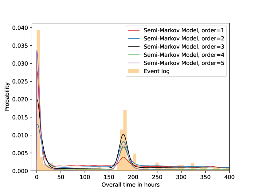
(a) The overall process execution time for the incident management system event log (BPI’13 incidents) and semi-Markov models discovered from this event log with threshold=0.001.

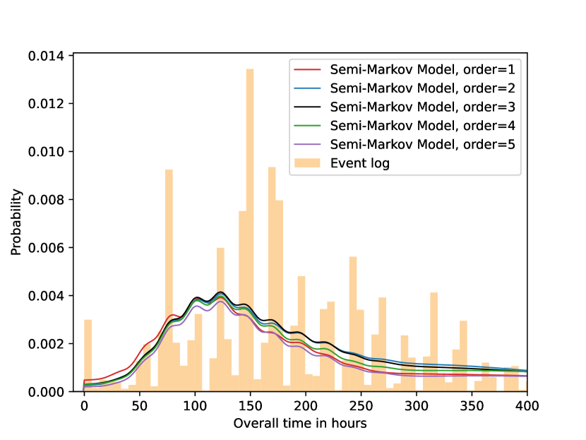
(b) The overall process execution time for the university travel expense claim system event log (DD’20) and semi-Markov models discovered from this event log with threshold=0.001.

Figure 12. Overall time distributions for event logs and semi-Markov models discovered from these event logs with threshold=0.001.

To calculate the (performance) accuracy of the discovered models we used Kullback–Leibler divergence. Kullback–Leibler divergence (KL divergence) (Kullback and Leibler, 1951) is a standard measure for relating distributions. For each discovered process model and a corresponding event log we calculated the KL divergence as:

$$KL(L,M)=\sum\limits_{t\in T}L(t)\ \ln\Big{(}\frac{L(t)}{M(t)}\Big{)}\ ,$$

where $t$ iterates over the set of bins (time intervals) $T$, $L(t)$ is the observed probability (obtained directly from the event log) and $M(t)$ is the discovered probability of being in time interval $t$. This divergence relates time distributions and represents the expected logarithmic difference between the observed and modeled probabilities.

Table 4 shows the mean and 95% CI for the KL divergence and reduction time of semi-Markov models built from the real-world event data with the thresholds set to 0.001 and 0.0001. KL divergence was computed for 20 equal intervals spanning all process times up to 1,000 hours. For each event log, each order $k$, and each threshold we ran 5 experiments. When the models were not discovered (using 8Gb of memory), the corresponding values were not provided.

Table 4. KL divergence (accuracy) and discovery time of models constructed from real-world event data.

Event log	Order $k$	KL divergence	Reduct. time (in sec.)	KL divergence	Reduct. time (in sec.)
		threshold = 0.001	threshold = 0.001	threshold = 0.0001	threshold = 0.0001
	1	0.1278$\pm$0.0000	0.57$\pm$0.04	0.1062 $\pm$0.0006	63.28$\pm$4.65
BPI'13	2	0.0833$\pm$0.0012	1.12$\pm$0.32	0.0539$\bf\pm$0.0009	768.16$\bf\pm$356.81
incidents	3	0.0777$\bf\pm$0.0004	4.45$\bf\pm$0.60	0.0667$\pm$0.0007	2,503.70$\pm$1,492.66
	4	0.5086$\pm$0.0342	40.30$\pm$1.83	–	–
	5	0.4445$\pm$0.0288	158.15$\pm$3.65	–	–
	1	0.2667$\pm$0.0000	0.67$\pm$0.04	0.2103$\pm$0.0000	540.04$\pm$2.64
	2	0.1725$\pm$0.0236	2.45$\pm$0.25	0.1371$\pm$0.0002	1,955.80$\pm$493.23
DD'20	3	0.1563$\bf\pm$0.0015	4.54$\bf\pm$0.20	0.1343$\bf\pm$0.0015	2,313.41$\bf\pm$589.93
	4	0.2067$\pm$0.0232	5.06$\pm$0.34	0.1504$\pm$0.0044	2,858.85$\pm$494.73
	5	0.3417$\pm$0.0540	4.56$\pm$0.26	0.1472$\pm$0.0075	1,616.34$\pm$300.88
	1	0.1463$\pm$0.0021	0.51$\pm$0.02	0.1254$\pm$0.0007	1,743.84$\pm$26.81
	2	0.1351$\bf\pm$0.0081	1.60$\bf\pm$0.41	0.1124$\pm$0.0008	1,630.16$\pm$655.07
RFP'20	3	0.1406$\pm$0.0035	2.70$\pm$0.29	0.1098$\pm$0.0007	1,352.59$\pm$139.70
	4	0.1376$\pm$0.0048	2.80$\pm$0.23	0.0915$\bf\pm$0.0008	1,097.27$\bf\pm$157.73
	5	0.1500$\pm$0.0065	4.68$\pm$0.37	0.1078$\pm$0.0054	2,216.98$\pm$447.70

Because of the pruning technique applied, the order in which states are reduced can affect the final distribution and its KL divergence from the event log. To mitigate this, we first removed states with the minimal $m_{1}\cdot m_{2}$ value, where $m_{1}$ is the number incoming transitions and $m_{2}$ is the number of outgoing transitions of a state. Additionally, removing less connected states first, allowed us to reduce the number of convolution operations and as a result get better KL divergence with smaller CIs as well as improve computational times. Note that KL divergence can still vary because a model can contain several states with minimal $m_{1}\cdot m_{2}$ values.

In Table 4, the best models in terms of accuracy for each of the event logs and each of the thresholds are highlighted in bold. Although, one might expect that the accuracy should increase as the order of discovered models increases, these results show that this is not always the case. This can be explained by the fact that the discovered models better capture traces that contain less process steps and hence require less number of convolutions and approximations regardless of the model order. Figure 13 presents the results for models discovered from RFP’20 event log with different thresholds. The models discovered with the threshold set to 0.0001 (Figure 13(b)) capture more peaks than the models discovered with the 0.001 threshold (Figure 13(a)), because they are more accurate and can better represent longer traces. However, note that for all the event logs and all the thresholds the second order models are more accurate than the first order models. This can be particularly observed for RFP’20 event log (Figure 13), where the first peaks are not fully captured by the first order models.

One more observation is that for BPI’13 incidents event log, the accuracy drops for $k$ larger than 3. In this case, the total number of Gaussians associated with all the transitions of higher-order models is large, and hence the pruning technique that reduces the accuracy will be applied at the last steps of the reduction. This results in higher-order models approximating the main peaks but not the minor time variations. As can be observed from Figure 14 (Figure 14 zooms in on the time distributions presented in Figure 12(a)), the distributions for semi-Markov models of order 4 and 5 are flatter than for other models and capture only the main peaks.

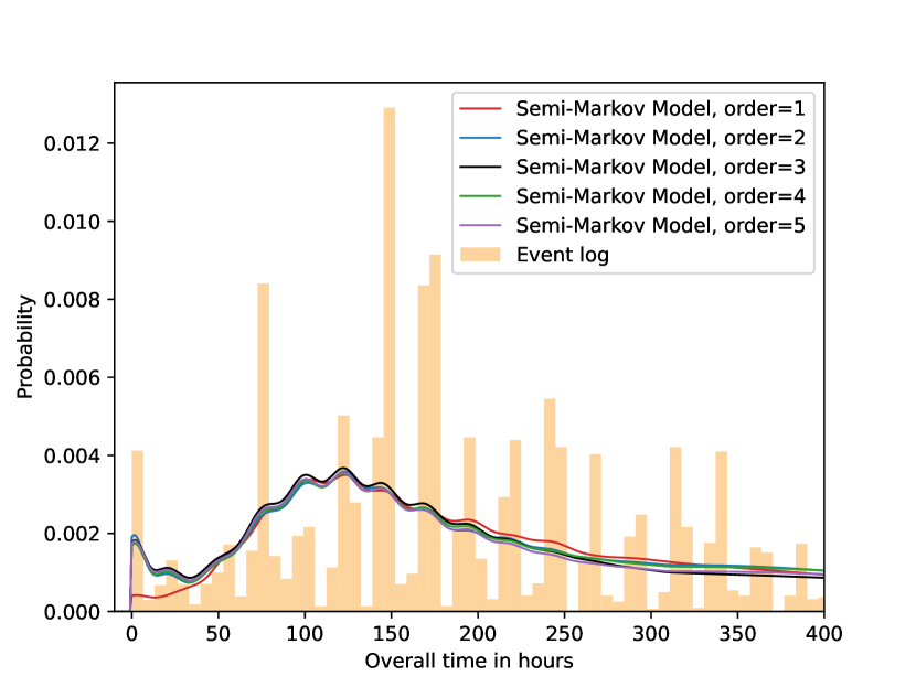
(a) The overall process execution time for the university travel expense claim system event log (RFP’20) and semi-Markov models discovered from this event log with threshold=0.001.

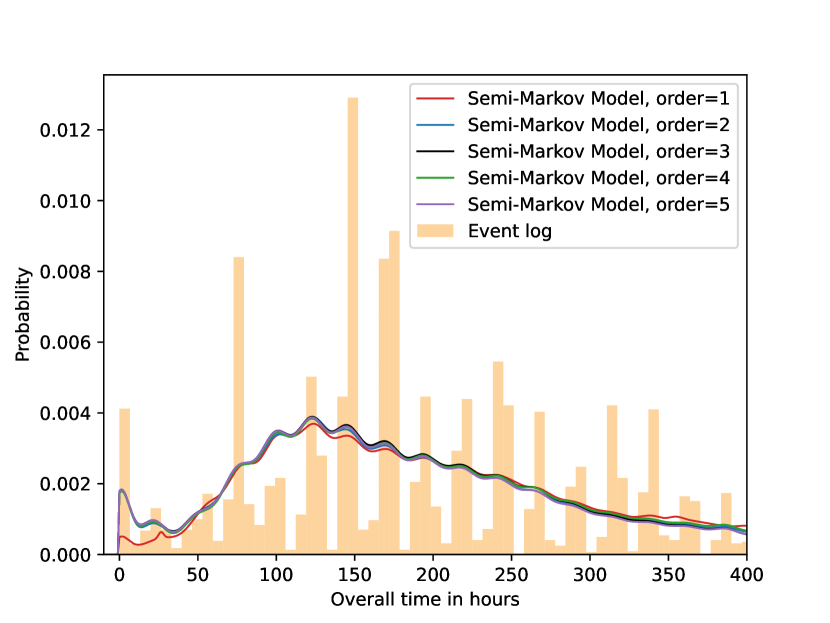
(b) The overall process execution time for the university travel expense claim system event log (RFP’20) and semi-Markov models discovered from this event log with threshold=0.0001.

Figure 13. Overall time distributions for the event log of the university travel expense claim system (RFP’20) and semi-Markov models discovered from this event log with different thresholds.

One might also expect that it takes more time to reduce large higher-order models. However, in some cases, the overall reduction time can vary because of the varying number of Gaussians associated with the transitions. So models with higher order $k$ may be equally fast or faster, though the trend for BPI’13 incidents and DD’20 event logs is that the computation times become larger for larger $k$. The combination of accuracy and computation times suggest that small values of $k$ between 1 and 2 are good choices for 0.001 and 0.0001 thresholds. The best choice for a particular application will vary. But in most cases these smaller values were, if not optimal, not far from.

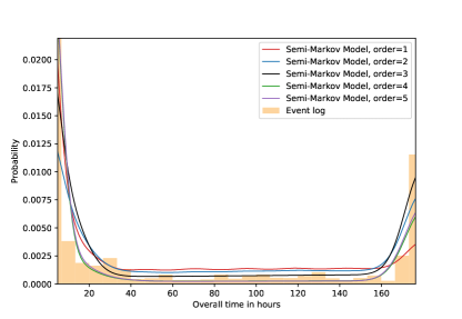
Figure 14. Zoomed-in time distributions for semi-Markov models discovered from BPI’13 incidents event log with the threshold set to 0.001 (see the original Figure 12(a)).

These experiments demonstrate the applicability of the proposed full analysis technique. It is shown that the best accuracy is in the range from 0.0539 to 0.1563 (the expected relations of observed and modelled processes’ durations are in the interval from 1.055 to 1.1692), and the most accurate overall time PDFs can be discovered in a reasonable amount of time (from 24 seconds to 46 minutes). To justify the results, we considered uniform distributions with means set to the logs’ mean times as a baseline and calculated the corresponding KL divergences. For the event logs BPI’13 incidents, DD’20, and RPF’20, the KL divergence between these event logs and the corresponding uniform distribution is 0.9006, 0.7105, and 0.5911, respectively. This demonstrates that the full analysis approach provides much more detailed results comparing with the baseline (uniform) approach.

5.4. Limitations of the full analysis technique and future work

The experimental results proved the applicability of the full analysis approach to real-world event data. However, we plan to further enhance the implementation by applying high performance and parallel computing techniques and considering lower thresholds. This will allow us to analyze additional event logs of the university travel expense claim system (International Declarations – ID’20 (van Dongen, 2020b), Prepaid Travel Costs – PTC’20 (van Dongen, 2020c), Travel Permit Data – TPD’20 (van Dongen, 2020e)) that contain longer traces (the median trace length for these event logs ranges from 8 to 11 events). We also plan to analyze the relationship between the order of the discovered models and performance accuracy at lower probability thresholds.

Two more event logs of the Volvo IT Belgium management system (BPI’13 open problems (Steeman, 2013c) and BPI’13 closed problems (Steeman, 2013a)) were disregarded because in these event logs durations vary from seconds to years and hence are incomparable with the results of the three analyzed sets. We leave consideration of these for future work.

6. Related Work

Various approaches for the discovery of stochastic models (e.g., Markov chains or stochastic Petri nets), are presented in the literature (Rogge-Solti et al., 2014; Rozinat et al., 2009; Anastasiou et al., 2012; Carrera and Jung, 2015; Kang and Zadorozhny, 2016; Augusto et al., 2018; Burke et al., 2021b, a). However, none of these approaches use mathematical tools offered by discovered models to analyze process performance. Paper (Anastasiou et al., 2012) presents a discovery method for inferring stochastic Petri nets with Erlang distributions from location tracking data. A technique for the discovery of $k$-order Markov chains from event logs is discussed in (Augusto et al., 2018). Hidden Markov models that capture both events and resources are discovered and analyzed in (Carrera and Jung, 2015). A method that discovers hidden semi-Markov models from event data is presented in (Kang and Zadorozhny, 2016), this method predicts only the most frequent sequences of states given the initial steps of the process. Techniques that discover stochastic Petri nets for their further simulation are presented in (Rogge-Solti et al., 2014; Rozinat et al., 2009). Papers (Burke et al., 2021b, a) propose methods that discover stochastic Petri nets and assess quality of the discovered models by relating them to the event logs. Besides stochastic process discovery, several methods for stochastic conformance checking were recently intorduced in (Augusto et al., 2018; Leemans et al., 2019; Bogdanov et al., 2022; Leemans and Polyvyanyy, 2020, 2023; Leemans et al., 2023; Burke et al., 2022).

Several performance analysis techniques proposed in the process mining context are based on the simulation of discovered models (Rogge-Solti and Weske, 2013, 2015; Vandenabeele et al., 2022; Rozinat et al., 2009; Camargo et al., 2020). A technique presented in (Camargo et al., 2020) is based on the discovery of BPMN (Business Process Model and Notation) models. These models are further enhanced by annotating activities with arbitrary time distribution functions inferred from event logs. This technique is focused on the adjustment of the discovery hyper-parameters to build accurate simulation models. A method to discover and simulate stochastic Petri nets with arbitrary distributed activity times is presented in (Rogge-Solti and Weske, 2013, 2015). A similar technique that considers normal distributions for activity execution times was proposed in (Rozinat et al., 2009). Paper (Vandenabeele et al., 2022) is focused on the discovery of stochastic Petri nets from a set of traces with prefixes similar to the analyzed trace to predict the remaining time by simulating the discovered model.

Methods for the remaining time prediction were introduced in (van der Aalst et al., 2011; van der Aalst et al., 2010a; Folino et al., 2012). These methods construct automata models from event logs annotating their states with remaining times and predict the remaining time for a trace by replaying it on a model. Paper (van der Aalst et al., 2011) is additionally focused on the analysis of different levels of models’ abstractions and discusses their impact on the remaining time prediction. Distinct automata models are constructed for different contexts (attributes in the event logs) in (Folino et al., 2012). These prediction methods are log-based and cannot be applied for what-if analysis.

Performance analysis through visualizations (Denisov et al., 2018; Adriansyah and Buijs, 2013; van Dongen. and Adriansyah, 2010; Leemans et al., 2018) allows end users to get valuable insights into the performance of the process. Techniques for projecting performance information onto Petri nets, hierarchical models, and fuzzy models, discovered from event logs are implemented in (Adriansyah and Buijs, 2013), (Leemans et al., 2018), and (van Dongen. and Adriansyah, 2010), respectively. Paper (Denisov et al., 2018) presents a visualization technique where event log activities are visualized as lines with start and end points corresponding to the begin and end activity times, and the color corresponding to the duration of the activity.

Closed-form solutions for the performance analysis of models discovered from event logs are presented in (van Zelst et al., 2021; Senderovich et al., 2019, 2018). However, these solutions differ from the methods presented in this paper. Paper (Senderovich et al., 2018) considers queuing networks and stochastic Petri nets with exponentially distributed execution times. An approach for deriving the most frequent sequences of states of hidden Markov models using Viterbi algorithm is applied in (Senderovich et al., 2019). Paper (van Zelst et al., 2021) presents an algorithm that derives only time intervals for activities and sub-processes, and does not consider probabilities of events. In this paper, we propose a general technique that calculates mean, as well as the density probability function for the overall process execution time in the presence of arbitrary time distributions and probabilities of events.

Techniques that analyze performance characteristics of stochastic process models outside the context of process mining are also presented in the literature. Paper (Kim et al., 2003) considers an approach for calculating $n$-th moments of process execution times for extended stochastic Petri nets using regular expressions. A relation between execution times in semi-Markov models and regular expressions was first discussed in (Csenki, 2008). A technique that calculates the execution time for block-structured stochastic time Petri nets is presented in (Carnevali et al., 2021). In this work, we propose, implement and test most general approach that constructs a probability density function of the overall process execution time, we also provide the exact closed-form solution for finding the mean process execution time.

7. Conclusion

The paper proposes express and full techniques for the performance analysis of stochastic process models discovered from event logs. These new techniques comparing to the existing performance analysis approaches used in process mining provide solutions that can be further applied to identify bottlenecks and review different scenarios of process execution without resorting to simulation. The express technique relates mean times of the process activities to the mean execution time of the process. The full analysis technique builds the probability density function (PDF) of the overall process execution time based on the PDFs of the process activities providing more detailed results. Both approaches are implemented and tested on real-world event data demonstrating their applicability in practice. For the full analysis technique, performance accuracy of the discovered models is additionally analyzed and discussed. As a future work, we plan to further enhance the implementation of the full analysis technique by leveraging high performance and parallel computing. We also plan to extend the full analysis approach by applying queuing theory to estimate the overall execution time in the presence of queues.

8. Acknowledgements

The authors are grateful to Alex Hu for his contributions to the idea of state removal order.

References

- (1)
- Adriansyah and Buijs (2013) Arya Adriansyah and Joos Buijs. 2013. Mining Process Performance from Event Logs. In Business Process Management Workshops. Springer Berlin Heidelberg, 217–218.
- Anastasiou et al. (2012) Nikolas Anastasiou, Tzu-Ching Horng, and William Knottenbelt. 2012. Deriving Generalised Stochastic Petri Net Performance Models from High-Precision Location Tracking Data. In 5th International ICST Conference on Performance Evaluation Methodologies and Tools. https://doi.org/10.4108/icst.valuetools.2011.245715
- Augusto et al. (2018) Adriano Augusto, Abel Armas-Cervantes, Raffaele Conforti, Marlon Dumas, Marcello La Rosa, and Daniel Reissner. 2018. Abstract-and-Compare: A Family of Scalable Precision Measures for Automated Process Discovery. In Business Process Management. Springer International Publishing, Cham, 158–175.
- Barron and Sheu (1991) Andrew Barron and Chyong-Hwa Sheu. 1991. Approximation of Density Functions by Sequences of Exponential Families. The Annals of Statistics 19, 3 (1991), 1347–1369.
- Berti et al. (2019) Alessandro Berti, Sebastiaan van Zelst, and Wil M. P. van der Aalst. 2019. Process Mining for Python (PM4Py): Bridging the Gap Between Process- and Data Science. In ICPM. Demo Track., Vol. 2374. 13–16.
- Bogdanov et al. (2022) Eli Bogdanov, Izack Cohen, and Avigdor Gal. 2022. Conformance Checking over Stochastically Known Logs. In Business Process Management Forum, Claudio Di Ciccio, Remco Dijkman, Adela del Río Ortega, and Stefanie Rinderle-Ma (Eds.). Springer International Publishing, Cham, 105–119.
- Burke et al. (2022) Adam T. Burke, Sander J.J. Leemans, Moe T. Wynn, Wil M.P van der Aalst, and Arthur H.M. ter Hofstede. 2022. Stochastic Process Model-Log Quality Dimensions: An Experimental Study. In 2022 4th International Conference on Process Mining (ICPM). 80–87. https://doi.org/10.1109/ICPM57379.2022.9980707
- Burke et al. (2021a) Adam T. Burke, Sander J. J. Leemans, and Moe T. Wynn. 2021a. Discovering Stochastic Process Models by Reduction and Abstraction. In Application and Theory of Petri Nets and Concurrency, Didier Buchs and Josep Carmona (Eds.). Springer International Publishing, Cham, 312–336.
- Burke et al. (2021b) Adam T. Burke, Sander J. J. Leemans, and Moe T. Wynn. 2021b. Stochastic Process Discovery by Weight Estimation. In Process Mining Workshops, Sander Leemans and Henrik Leopold (Eds.). Springer International Publishing, Cham, 260–272.
- Camargo et al. (2020) Manuel Camargo, Marlon Dumas, and Oscar González-Rojas. 2020. Automated discovery of business process simulation models from event logs. Decision Support Systems 134 (2020), 113284. https://doi.org/10.1016/j.dss.2020.113284
- Carnevali et al. (2021) Laura Carnevali, Marco Paolieri, Riccardo Reali, and Enrico Vicario. 2021. Compositional Safe Approximation of Response Time Distribution of Complex Workflows. In Quantitative Evaluation of Systems, Alessandro Abate and Andrea Marin (Eds.). Springer International Publishing, Cham, 83–104.
- Carrera and Jung (2015) Berny Carrera and Jae-Yoon Jung. 2015. Constructing Probabilistic Process Models Based on Hidden Markov Models for Resource Allocation. In Business Process Management Workshops. Springer, 477–488.
- Ching et al. (2004) Wai-Ki Ching, Eric Fung, and Michael Ng. 2004. Higher‐order Markov chain models for categorical data sequences. Naval Research Logistics 51 (2004).
- Csenki (2008) Attila Csenki. 2008. Flowgraph Models in Reliability and Finite Automata. IEEE Transactions on Reliability 57, 2 (2008), 355–359. https://doi.org/10.1109/TR.2008.920865
- Denisov et al. (2018) Vadim Denisov, Dirk Fahland, and Wil M. P. van der Aalst. 2018. Unbiased, Fine-Grained Description of Processes Performance from Event Data. In Business Process Management - 16th International Conference, BPM 2018, Sydney, NSW, Australia, September 9-14, 2018, Proceedings (Lecture Notes in Computer Science, Vol. 11080), Mathias Weske, Marco Montali, Ingo Weber, and Jan vom Brocke (Eds.). Springer, 139–157. https://doi.org/10.1007/978-3-319-98648-7_9
- Folino et al. (2012) Francesco Folino, Massimo Guarascio, and Luigi Pontieri. 2012. Discovering Context-Aware Models for Predicting Business Process Performances. In On the Move to Meaningful Internet Systems: OTM 2012, Robert Meersman, Hervé Panetto, Tharam Dillon, Stefanie Rinderle-Ma, Peter Dadam, Xiaofang Zhou, Siani Pearson, Alois Ferscha, Sonia Bergamaschi, and Isabel F. Cruz (Eds.). Springer Berlin Heidelberg, Berlin, Heidelberg, 287–304.
- Hopcroft et al. (2007) John E. Hopcroft, Rajeev Motwani, and Jeffrey D. Ullman. 2007. Introduction to Automata Theory, Languages, and Computation, 3rd Edition. Addison-Wesley.
- ISO 9000:2005 (2005) ISO 9000:2005 2005. Quality management systems — Fundamentals and vocabulary. Standard. International Organization for Standardization.
- Kang and Zadorozhny (2016) Yihuang Kang and Vladimir Zadorozhny. 2016. Process Discovery Using Classification Tree Hidden Semi-Markov Model. In IRI. 361–368. https://doi.org/10.1109/IRI.2016.55
- Kim et al. (2003) Dong Sung Kim, Hong-Ju Moon, Je-Hyeong Bahk, Wook Hyun Kwon, and Zygmunt J. Haas. 2003. Efficient Computations for Evaluating Extended Stochastic Petri Nets using Algebraic Operations. International Journal of Control Automation and Systems 1 (2003), 431–443.
- Kullback and Leibler (1951) Solomon Kullback and Richard A. Leibler. 1951. On Information and Sufficiency. Annals of Mathematical Statistics 22 (1951), 79–86.
- Leemans et al. (2018) Maikel Leemans, Wil M. P. van der Aalst, and Mark G. J. van den Brand. 2018. Hierarchical Performance Analysis for Process Mining. In Proceedings of the 2018 International Conference on Software and System Process (Gothenburg, Sweden) (ICSSP ’18). Association for Computing Machinery, New York, NY, USA, 96–105. https://doi.org/10.1145/3202710.3203151
- Leemans and Polyvyanyy (2023) Sander J.J. Leemans and Artem Polyvyanyy. 2023. Stochastic-aware precision and recall measures for conformance checking in process mining. Information Systems 115 (2023), 102197. https://doi.org/10.1016/j.is.2023.102197
- Leemans et al. (2023) Sander J. J. Leemans, Fabrizio M. Maggi, and Marco Montali. 2023. Enjoy the Silence: Analysis of Stochastic Petri Nets with Silent Transitions. arXiv:2306.06376
- Leemans and Polyvyanyy (2020) Sander J. J. Leemans and Artem Polyvyanyy. 2020. Stochastic-Aware Conformance Checking: An Entropy-Based Approach. In Advanced Information Systems Engineering, Schahram Dustdar, Eric Yu, Camille Salinesi, Dominique Rieu, and Vik Pant (Eds.). Springer International Publishing, Cham, 217–233.
- Leemans et al. (2019) Sander J. J. Leemans, Anja F. Syring, and Wil M. P. van der Aalst. 2019. Earth Movers’ Stochastic Conformance Checking. In Business Process Management Forum (Lecture Notes in Business Information Processing, Vol. 360). Springer, 127–143. https://doi.org/10.1007/978-3-030-26643-1_8
- Polyvyanyy et al. (2020) Artem Polyvyanyy, Andreas Solti, Matthias Weidlich, Claudio Di Ciccio, and Jan Mendling. 2020. Monotone Precision and Recall Measures for Comparing Executions and Specifications of Dynamic Systems. ACM Trans. Softw. Eng. Methodol. 29, 3, Article 17 (2020), 41 pages. https://doi.org/10.1145/3387909
- Pyke (1961) Ronald Pyke. 1961. Markov Renewal Processes with Finitely Many States. The Annals of Mathematical Statistics 32, 4 (1961), 1243–1259. https://doi.org/10.1214/aoms/1177704864
- Rogge-Solti et al. (2014) Andreas Rogge-Solti, Wil M. P. van der Aalst, and Mathias Weske. 2014. Discovering stochastic Petri nets with arbitrary delay distributions from event logs. In Business Process Management Workshops : BPM 2013 International Workshops. Springer, 15–27. https://doi.org/10.1007/978-3-319-06257-0_2
- Rogge-Solti and Weske (2013) Andreas Rogge-Solti and Mathias Weske. 2013. Prediction of Remaining Service Execution Time Using Stochastic Petri Nets with Arbitrary Firing Delays. In Service-Oriented Computing, Samik Basu, Cesare Pautasso, Liang Zhang, and Xiang Fu (Eds.). Springer Berlin Heidelberg, Berlin, Heidelberg, 389–403.
- Rogge-Solti and Weske (2015) Andreas Rogge-Solti and Mathias Weske. 2015. Prediction of business process durations using non-Markovian stochastic Petri nets. Information Systems 54 (2015), 1–14. https://doi.org/10.1016/j.is.2015.04.004
- Ross (1985) Sheldon Ross. 1985. Introduction to Probability Models (third ed.). Academic Press, Orlando, Florida, USA.
- Rozinat et al. (2009) Anne Rozinat, Ronny S. Mans, Minseok Song, and Wil M. P. van der Aalst. 2009. Discovering simulation models. Inf. Systems 34, 3 (2009), 305–327.
- Senderovich et al. (2018) Arik Senderovich, Alexander Shleyfman, Matthias Weidlich, Avigdor Gal, and Avishai Mandelbaum. 2018. To aggregate or to eliminate? Optimal model simplification for improved process performance prediction. Information Systems 78 (2018), 96–111. https://doi.org/10.1016/j.is.2018.04.003
- Senderovich et al. (2019) Arik Senderovich, Matthias Weidlich, and Avigdor Gal. 2019. Context-aware temporal network representation of event logs: Model and methods for process performance analysis. Information Systems 84 (2019), 240–254. https://doi.org/10.1016/j.is.2019.04.004
- Steeman (2013a) Ward Steeman. 2013a. BPI Challenge 2013, closed problems. https://doi.org/10.4121/uuid:c2c3b154-ab26-4b31-a0e8-8f2350ddac11
- Steeman (2013b) Ward Steeman. 2013b. BPI Challenge 2013, incidents. https://doi.org/10.4121/uuid:500573e6-accc-4b0c-9576-aa5468b10cee
- Steeman (2013c) Ward Steeman. 2013c. BPI Challenge 2013, open problems. https://doi.org/10.4121/uuid:3537c19d-6c64-4b1d-815d-915ab0e479da
- van der Aalst et al. (2002) Wil M. P. van der Aalst, Alexander Hirnschall, and Eric Verbeek. 2002. An Alternative Way to Analyze Workflow Graphs. In Advanced Information Systems Engineering. Springer Berlin Heidelberg, 535–552.
- van der Aalst et al. (2010a) Wil M. P. van der Aalst, Maja Pesic, and Minseok Song. 2010a. Beyond Process Mining: From the Past to Present and Future. In Advanced Information Systems Engineering, Barbara Pernici (Ed.). Springer Berlin Heidelberg, Berlin, Heidelberg, 38–52.
- van der Aalst et al. (2010b) Wil M. P. van der Aalst, Vladimir Rubin, Eric Verbeek, Boudewijn van Dongen, Ekkart Kindler, and Christian Günther. 2010b. Process mining: a two-step approach to balance between underfitting and overfitting. SoSyM 9, 1 (2010), 87.
- van der Aalst et al. (2011) Wil M. P. van der Aalst, Helen Schonenberg, and Minseok Song. 2011. Time prediction based on process mining. Information Systems 36, 2 (2011), 450–475. https://doi.org/10.1016/j.is.2010.09.001 Special Issue: Semantic Integration of Data, Multimedia, and Services.
- van der Aalst (2016) Wil W. M. van der Aalst. 2016. Process Mining: Data Science in Action. Springer. https://doi.org/10.1007/978-3-662-49851-4
- van Dongen (2020a) Boudewijn van Dongen. 2020a. BPI Challenge 2020: Domestic Declarations. https://doi.org/10.4121/uuid:3f422315-ed9d-4882-891f-e180b5b4feb5
- van Dongen (2020b) Boudewijn van Dongen. 2020b. BPI Challenge 2020: International Declarations. https://doi.org/10.4121/uuid:2bbf8f6a-fc50-48eb-aa9e-c4ea5ef7e8c5
- van Dongen (2020c) Boudewijn van Dongen. 2020c. BPI Challenge 2020: Prepaid Travel Costs. https://doi.org/10.4121/uuid:5d2fe5e1-f91f-4a3b-ad9b-9e4126870165
- van Dongen (2020d) Boudewijn van Dongen. 2020d. BPI Challenge 2020: Request For Payment. https://doi.org/10.4121/uuid:895b26fb-6f25-46eb-9e48-0dca26fcd030
- van Dongen (2020e) Boudewijn van Dongen. 2020e. BPI Challenge 2020: Travel Permit Data. https://doi.org/10.4121/uuid:ea03d361-a7cd-4f5e-83d8-5fbdf0362550
- van Dongen. and Adriansyah (2010) Boudewijn van Dongen. and Arya Adriansyah. 2010. Process Mining: Fuzzy Clustering and Performance Visualization. In Business Process Management Workshops. Springer Berlin Heidelberg, 158–169.
- van Zelst et al. (2021) Sebastiaan J. van Zelst, Luis F. R. Santos, and Wil M. P. van der Aalst. 2021. Data-Driven Process Performance Measurement and Prediction: A Process-Tree-Based Approach. In Intelligent Information Systems, Selmin Nurcan and Axel Korthaus (Eds.). Springer International Publishing, Cham, 73–81.
- Vandenabeele et al. (2022) Jarne Vandenabeele, Gilles Vermaut, Jari Peeperkorn, and Jochen De Weerdt. 2022. Enhancing Stochastic Petri Net-based Remaining Time Prediction using k-Nearest Neighbors. CEUR Workshop Proceedings 3167 (2022), 9 – 24.
- Weijters et al. (2006) Anton J. M. M. Weijters, Wil M. P. van der Aalst, and Ana K. Alves de Medeiros. 2006. Process Mining with the Heuristics Miner-algorithm. Eindhoven.
- Wilson and Wragg (1972) G. Wilson and A. Wragg. 1972. Numerical Methods for Approximating Continuous Probability Density Functions, over , Using Moments.