On the Calculation of the Variance of Algebraic Variables in Power System Dynamic Models with Stochastic Processes

Abstract

This letter presents a technique to calculate the variance of algebraic variables of power system models represented as a set of stochastic differential-algebraic equations. The technique utilizes the solution of a Lyapunov equation and requires the calculation of the state matrix of the system. The IEEE 14-bus system serves to demonstrate the accuracy of the proposed technique over a wide range of variances of stochastic processes. The accuracy is evaluated by comparing the results with those obtained with Monte Carlo time domain simulations. Finally, a case study based on a 1479-bus dynamic model of the all-island Irish transmission system shows the computational efficiency of the proposed approach compared to the Monte Carlo method.

I Introduction

Modern power systems are subjected to stochastic processes due to the high penetration of non-synchronous generation such as wind and photo-voltaic. Stochastic load consumption is another relevant source of noise, especially at the distribution level. It is important to study the impact of stochastic processes to estimate the probability that physical limits such as voltage insulation ratings of a substation, the thermal limits of the lines/transformers, are violated in normal operation. This letter focuses precisely on this point and proposes an efficient technique that, given the properties of the noise sources, evaluates the variance of all state and algebraic variables of power system dynamic models.

The dynamic performance of a power system with inclusion of stochastic processes can be conveniently studied through Stochastic Differential Algebraic Equations [1]. These SDAEs are non-linear and can have high dimensionality for large power systems. The use of numerical schemes for their integration is thus unavoidable. The stochastic terms require a significant extra computational burden to solve the integration [2]. Moreover, SDAEs have to be studied with a Monte Carlo method, i.e., several hundreds or even thousands of times, to properly estimate the statistical properties of the system variables, such their probability distribution and variance.

A number of techniques are available in the literature that provide the statistical properties in stationary conditions of the state variables, e.g. [3] and [4]. These methods are based on the properties of the Fokker-Planck equation and the solution of the Lyapunov equation. This letter further elaborates on this approach and proposes the utilization of a simple, yet effective linearized method to calculate the statistical properties of the algebraic variables of power systems without the need to perform cumbersome time domain simulations.

II Power System Model with Noise

The power system model considered in this work is described by the following set of index-1 SDAEs:

$$\dot{\boldsymbol{x}} =\boldsymbol{f}(\boldsymbol{x},\boldsymbol{y},\boldsymbol{\eta})\,,$$ (1)

$$\boldsymbol{0}_{m,1} =\boldsymbol{g}(\boldsymbol{x},\boldsymbol{y},\boldsymbol{\eta})\,,$$ (2)

$$\dot{\boldsymbol{\eta}} =\boldsymbol{a}(\boldsymbol{\eta})+\boldsymbol{\rm B}(\boldsymbol{\eta})\,\boldsymbol{\xi}\,.$$ (3)

Equations (1)-(2) describe the conventional deterministic power system models such as transmission lines, generators and controllers. Vector $\boldsymbol{f}:\mathbb{R}^{n+m+p}\mapsto\mathbb{R}^{n}$ defines the deterministic differential equations; vector $\boldsymbol{g}:\mathbb{R}^{n+m+p}\mapsto\mathbb{R}^{m}$ defines the algebraic equations; $\boldsymbol{x}\in\mathbb{R}^{n}$ is the vector of the deterministic state variables and $\boldsymbol{y}\in\mathbb{R}^{m}$ is the vector of the algebraic variables. Equation (3) defines the behavior of the stochastic processes $\boldsymbol{\eta}\in\mathbb{R}^{p}$, where $\boldsymbol{\xi}\in\mathbb{R}^{q}$ is the white noise vector, i.e., the vector of the formal time derivatives of the Wiener processes. Vector $\boldsymbol{\eta}$ represents the fluctuations of loads and renewable energy sources such as wind and solar power plants. Equation (3) is composed of two terms: the drift $\boldsymbol{a}:\mathbb{R}^{p}\mapsto\mathbb{R}^{p}$ and the diffusion term $\boldsymbol{\rm B}:\mathbb{R}^{p}\mapsto\mathbb{R}^{p}\times\mathbb{R}^{q}$. The elements of matrix $\boldsymbol{\rm B}$ are, in general, nonlinear functions of $\boldsymbol{\eta}$ to account for distributions other than Gaussian [5]. However, for short-term analysis and/or small fluctuations, one can assume normal distributions, which lead to a constant diffusion matrix $\boldsymbol{B}$ [1].

In the general case, $p\neq q$. This feature allows modeling correlated processes [6]. If $p=q$ and $\boldsymbol{\rm B}$ is a diagonal matrix, then the processes $\boldsymbol{\eta}$ are fully uncorrelated. In the following, without lack of generality, the elements of $\boldsymbol{\eta}$ are assumed to be uncorrelated and with bounded variance. The latter property has been observed in the measurements of the noise sources of power systems, as discussed in [1] and references therein. A widely accepted model with bounded variance is the mean-reverted process, which has a linear drift term of the form:

$$a_{k}(\eta_{k})=\alpha_{k}(\mu_{k}-\eta_{k})\,,\qquad k=1,2,\dots,p\,,$$ (4)

where $\alpha_{k}$ is the mean reversion speed, which defines the autocorrelation of the process, and $\mu_{k}$ is the average value of the process. If a mean-reverted drift (4) is coupled with a constant diffusion, say $b_{k}$, one obtains a normally distributed Ornstein-Uhlenbeck (OU) process with variance:

$${\rm var}(\eta_{k})=\sigma^{2}_{k}={b^{2}_{k}}/({2\alpha_{k}})\,,\qquad k=1,2,\dots,p\,,$$ (5)

where $\sigma_{k}$ is the standard deviation of the $k$-th process. Note also that $b_{k}$ is the $k$-th diagonal element of the diffusion matrix $\boldsymbol{\rm B}$.

III Calculation of the Variance of Algebraic Variables

The starting point of the proposed technique to calculate the variances of the algebraic variables $\boldsymbol{y}$ is the set of SDAEs linearized at the equilibrium point $(\boldsymbol{x}_{o},\boldsymbol{y}_{o},\boldsymbol{\eta}_{o})$ as per Method I described in [4], i.e., a point for which (2) are satisfied and $\dot{\boldsymbol{x}}=\boldsymbol{0}_{n,1}$ and $\boldsymbol{a}(\boldsymbol{\eta}_{o})=\boldsymbol{0}_{p,1}$. The linearization of (1)-(3) gives:

$$\begin{bmatrix}\dot{\tilde{\boldsymbol{x}}}\\ \boldsymbol{0}_{m,1}\\ \dot{\tilde{\boldsymbol{\eta}}}\end{bmatrix}=\begin{bmatrix}\boldsymbol{f}_{\boldsymbol{x}}&\boldsymbol{f}_{\boldsymbol{y}}&\boldsymbol{f}_{\boldsymbol{\eta}}\\ \boldsymbol{g}_{\boldsymbol{x}}&\boldsymbol{g}_{\boldsymbol{y}}&\boldsymbol{g}_{\boldsymbol{\eta}}\\ \boldsymbol{0}_{p,n}&\boldsymbol{0}_{p,m}&\boldsymbol{a}_{\boldsymbol{\eta}}\\ \end{bmatrix}\begin{bmatrix}\tilde{\boldsymbol{x}}\\ \tilde{\boldsymbol{y}}\\ \tilde{\boldsymbol{\eta}}\end{bmatrix}+\begin{bmatrix}\boldsymbol{0}_{n,q}\\ \boldsymbol{0}_{m,q}\\ \boldsymbol{\rm B}(\boldsymbol{\eta}_{o})\end{bmatrix}\boldsymbol{\xi}\,,$$ (6)

where $\boldsymbol{f}_{\boldsymbol{x}}$, $\boldsymbol{f}_{\boldsymbol{y}}$, $\boldsymbol{f}_{\boldsymbol{\eta}}$, $\boldsymbol{g}_{\boldsymbol{x}}$, $\boldsymbol{g}_{\boldsymbol{y}}$, $\boldsymbol{g}_{\boldsymbol{\eta}}$, $\boldsymbol{a}_{\boldsymbol{\eta}}$ are the Jacobian matrices of the system calculated at $(\boldsymbol{x}_{o},\boldsymbol{y}_{o},\boldsymbol{\eta}_{o})$. $\tilde{\boldsymbol{x}}$ and $\tilde{\boldsymbol{\eta}}$ represent the deterministic and the stochastic states of the linearized system. Eliminating the algebraic variables from (6) and defining $\tilde{\boldsymbol{z}}=[\tilde{\boldsymbol{x}}{\color[rgb]{1,0,0}{}^{\mathrm{T}}},\tilde{\boldsymbol{\eta}}{\color[rgb]{1,0,0}{}^{\mathrm{T}}}]^{T}$ leads to a set of linear stochastic differential equations, as follows:

$$\begin{bmatrix}\dot{\tilde{\boldsymbol{x}}}\\ \dot{\tilde{\boldsymbol{\eta}}}\end{bmatrix} =\begin{bmatrix}\boldsymbol{f}_{\boldsymbol{x}}-\boldsymbol{f}_{\boldsymbol{y}}\boldsymbol{g}^{\boldsymbol{-}1}_{\boldsymbol{y}}\boldsymbol{g}_{\boldsymbol{x}}&\boldsymbol{f}_{\boldsymbol{\eta}}-\boldsymbol{f}_{\boldsymbol{y}}\boldsymbol{g}^{\boldsymbol{-}1}_{\boldsymbol{y}}\boldsymbol{g}_{\boldsymbol{\eta}}\\ \boldsymbol{0}_{p,n}&\boldsymbol{a}_{\boldsymbol{\eta}}\\ \end{bmatrix}\begin{bmatrix}\tilde{\boldsymbol{x}}\\ \tilde{\boldsymbol{\eta}}\end{bmatrix}+\begin{bmatrix}\boldsymbol{0}_{n,q}\\ \boldsymbol{\rm B}(\boldsymbol{\eta}_{o})\end{bmatrix}\boldsymbol{\xi}$$

$$=\boldsymbol{\rm A}_{o}\,\tilde{\boldsymbol{z}}+\boldsymbol{\rm B}_{o}\,\boldsymbol{\xi}\,.$$ (7)

Based on the Fokker-Planck equation, the probability distribution $\boldsymbol{\varpi}(\tilde{\boldsymbol{z}})$ of all state variables in stationary condition satisfies [3]:

$$\boldsymbol{\varpi}(\tilde{\boldsymbol{z}})=({\rm det}\mid 2\pi\boldsymbol{\rm C}\mid)^{-1/2}\cdot{\rm exp}\bigg{(}-\frac{1}{2}\tilde{\boldsymbol{z}}^{\mathrm{T}}\boldsymbol{\rm C}^{\boldsymbol{-}1}\tilde{\boldsymbol{z}}\bigg{)}\,,$$ (8)

where $\boldsymbol{\rm C}$ is the covariance matrix of the state variables in (7). Matrix $\boldsymbol{\rm C}$ is symmetric and satisfies the Lyapunov equation:

$$\boldsymbol{\rm A}_{o}\boldsymbol{\rm C}+\boldsymbol{\rm C}\boldsymbol{\rm A}_{o}^{\mathrm{T}}=-\boldsymbol{\rm B}_{o}\boldsymbol{\rm B}_{o}^{\mathrm{T}}\,,$$ (9)

which is a special case of the Riccati equation. The diagonal elements of $\boldsymbol{\rm C}$ are the steady-state variances of the components of the state variables $\tilde{\boldsymbol{z}}$. In particular, if the OU processes $\boldsymbol{\eta}$ are not correlated, the last $p$ diagonal elements of $\boldsymbol{\rm C}$ are given by (5) where $a_{k}$ and $b_{k}$ are the $k$-th diagonal elements of $\boldsymbol{a}_{\boldsymbol{\eta}}$ and $\boldsymbol{\rm B}_{o}$, respectively, and $\sigma_{k}^{2}$ are the variances of the $p$ stochastic processes $\tilde{\boldsymbol{\eta}}$. The interested reader can refer to [4] for a comprehensive discussion on the numerical solution of (9).

From (7), we observe that $\tilde{\boldsymbol{x}}$ can be written as a linear combination of the entries of $\tilde{\boldsymbol{z}}$. Hence, also the elements of $\tilde{\boldsymbol{x}}$ are Gaussian processes. Furthermore, the covariance matrix $\boldsymbol{\rm K}$ of the small-signal algebraic variables can be written as [7]:

$$\boldsymbol{\rm K}=\boldsymbol{\rm G}_{o}\,\boldsymbol{\rm C}\,\boldsymbol{\rm G}_{o}^{\mathrm{T}}\,,$$ (10)

where

$$\boldsymbol{\rm G}_{o}=-\boldsymbol{g}^{-1}_{\boldsymbol{y}}\begin{bmatrix}\boldsymbol{g}_{\boldsymbol{x}}&\boldsymbol{g}_{\boldsymbol{\eta}}\end{bmatrix}.$$ (11)

The diagonal elements of $\boldsymbol{\rm K}$ are the sought variances of the algebraic variables $\tilde{\boldsymbol{y}}$.

Note that if $p\ll n$, i.e., the number of noise sources is much smaller than the number of state variables, the covariance matrices $\boldsymbol{\rm C}$ and hence $\boldsymbol{\rm K}$ might not be full rank. A zero element in the $k$-th position of the diagonal of $\boldsymbol{\rm C}$ ($\boldsymbol{\rm K}$) indicates that the associated $\tilde{x}_{k}$ ($\tilde{y}_{k}$) are not affected by noise. In this case, the vector of stochastic processes $\tilde{\boldsymbol{z}}$ is said to be degenerate [8].

IV Case Studies

This section illustrates the accuracy and numerical efficiency of the method in Section III to calculate the variances of algebraic variables of the power system. All results are compared to the ones obtained through Monte Carlo (MC) time domain simulations. The power systems utilized in this case study are the IEEE 14-bus system, and the all-island Irish transmission system (AIITS). The MC simulations are performed exploiting parallelism on 2 Intel® Xeon® CPUs at 2.20GHz with 20-cores each, running a Linux OS that exploits core virtualization (hypertrading). This means that at most 80 realizations were solved in parallel for each MC simulation. Equation (9) is solved using the open-source library SLICOT [9], whereas time domain simulations are carried out with Dome [10]. In the remainder of this section, the systems of equations (9) and (10) are referred to as Lyapunov Equation Method (LEM).

In both power systems, the sources of noise are modeled as OU processes and included in the loads and, for the AIITS, also in the wind speeds. Load consumption is modeled as voltage dependent incorporating stochastic processes:

$$p_{\rm L}(t) =(p_{{\rm L}0}+\eta_{p}(t))(v(t)/v_{0})^{\gamma}\,,$$ (12)

$$q_{\rm L}(t) =(q_{{\rm L}0}+\eta_{q}(t))(v(t)/v_{0})^{\gamma}\,,$$

$$v_{\rm W}(t) =v_{{\rm W}0}+\eta_{w}(t)\,,$$

where $p_{{\rm L}0}$ and $q_{{\rm L}0}$ are the active and reactive power consumption at time $t=0$; $v(t)$ is the magnitude of the bus voltage at the load bus; $v_{0}$ is the voltage magnitude at the load bus at the start of the simulation; $\gamma$ defines the load voltage dependence; and $\eta_{p}$ and $\eta_{q}$ are OU stochastic processes with drift and diffusion terms defined as in (4) and (5), respectively. $\gamma=2$ is utilized in all simulations.

In (12) $v_{{\rm W}0}$ is the initial wind speed; and $\eta_{w}$ is a stochastic process characterized by a Weibull distribution. This is obtained using the technique described in [11], namely, using the same drift term defined as in (4) and a nonlinear diffusion function $b_{w}(\eta_{w})$, as follows:

$$a_{w}(\eta_{w}) =\alpha_{w}(\mu_{w}-\eta_{w})$$ (13)

$$b_{w}(\eta_{w}) =\sqrt{b_{1}(\eta_{w})b_{2}(\eta_{w})}\,,$$

where

$$\mu_{w} =\lambda\Gamma\left(1+\kappa^{-1}\right)\,,$$

$$b_{1}(\eta_{w}) =2\alpha_{w}\,\eta_{w}\,c_{1}\frac{\lambda}{{\kappa}}\left(c_{2}(\eta_{w})\right)^{-\kappa}\,,$$

$$b_{2}(\eta_{w}) =\kappa\exp\left(c_{2}^{\kappa}(\eta_{w})\right)\Gamma\left(1+c_{1},c_{2}^{\kappa}(\eta_{w})\right)-\Gamma\left(c_{1}\right)\,.$$

In the above equations, $c_{1}=1/\kappa$ and $c_{2}(\eta_{w})=\eta_{w}/\lambda$; $\alpha_{w}$ is the autocorrelation coefficient; $\kappa$ and $\lambda$ are the shape and scale parameters, respectively, of the Weibull distribution; and $\Gamma(\cdot)$ and $\Gamma(\cdot,\cdot)$ are the Gamma function and the Incomplete Gamma functions, respectively.

The stochastic processes are modeled with the following parameters: ${\alpha_{p}=\alpha_{q}=\alpha_{w}=0.01}\,\text{s}^{-1}$; ${\sigma(\eta_{p})=0.05\,p_{\rm L0}}$; ${\sigma(\eta_{q})=0.05\,q_{\rm L0}}$ and ${\sigma(\eta_{w})=0.05\,v_{\rm W0}}$. The integration of the deterministic part of SDAEs is performed by the implicit trapezoidal method with the ${\Delta t=0.01\,\text{s}}$ time step. The OU processes are integrated using the Euler-Maruyama method with ${h=0.01\,\text{s}}$ step size.

IV-A IEEE 14-Bus System

The IEEE 14-bus system contains 14 buses with 11 loads, 20 lines/transformers, and 5 synchronous machines. The synchronous generators are described by a sixth-order model, and are equipped with turbine governors and IEEE Type-I automatic voltage regulators. An automatic generation control is also included in the model. The IEEE 14-bus system is modified by including a wind power plant connected to bus 5. All device models and data can be found in [12].

The IEEE 14-bus system is first simulated using the MC approach. MC simulations require the selection of two parameters, namely, the final simulation time $t_{f}$ and the number $N$ of realizations of $\boldsymbol{\eta}$. These parameters decide how the stationary conditions are reached and, hence, directly impact the accuracy of the statistical properties, such as the standard deviation, of the variables.

The choice of the value of $t_{f}$ depends principally on the parameters $\alpha_{i}$ of the underlying processes and can be heuristically estimated as $t_{f}=2/\min\{\alpha_{i}\}$. As a proof of concept, Fig. 1 shows the time evaluation of $\sigma_{\eta}$ for different values of $\alpha$. Figure 1 shows that the stationarity of $\sigma_{\eta}$ strongly depends on $\alpha$ (top panel) and is independent from $\sigma_{\eta}$ at stationary conditions (bottom panel). More details on the evolution of the standard deviation of the power system variables can be found in [13]. In the simulations carried out for this case study, the smallest $\alpha_{i}$ are of the order of $10^{-2}$ s and Fig. 1 confirms that a simulation time of $200$ s is adequate to allow for all stochastic processes to reach stationarity.

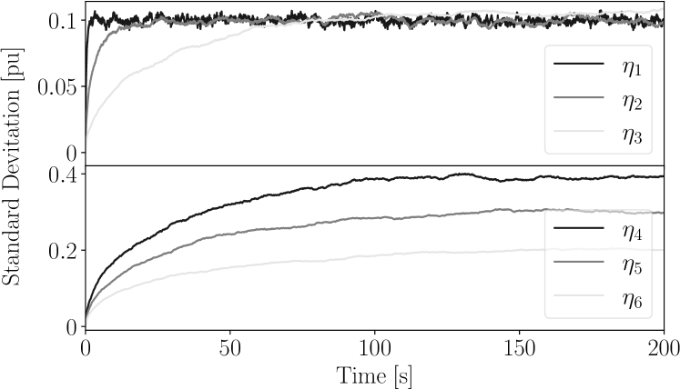
Figure 1: Standard deviation of $\eta$ as a function of time, where the parameters are defined such that $\sigma(\eta_{1})=\sigma(\eta_{2})=\sigma(\eta_{3})=0.1$ with $\alpha_{1}=1$ s^-1; $\alpha_{2}=0.1$ s^-1; and $\alpha_{3}=0.01$ s^-1, and $\sigma(\eta_{4})=0.4$; $\sigma(\eta_{5})=0.3$; $\sigma(\eta_{6})=0.2$ with $\alpha_{4}=\alpha_{5}=\alpha_{6}=0.01$ s^-1.

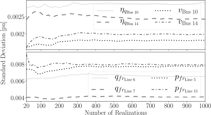
Figure 2: Standard deviation of variables as a function of the number of realizations of $\boldsymbol{\eta}$.

The second parameter to choose is the number of realizations $N$ for which the estimated value of $\sigma_{\eta}$ is reliable enough to be independent of the specific realizations of the stochastic processes. The best value of $N$ is determined by calculating the average $\sigma_{\eta}$ of each process at $t=200$ s as a function of $N$, as shown in Fig. 2. This figure shows that as $N$ increases, the standard deviation of $\boldsymbol{\eta}$ and of other system variables converges towards a constant value. Based on these results, $N=1000$ appears sufficient to obtain accurate stationary conditions with the MC approach.

Next, we compare the values of standard deviation of the power system variables for the IEEE 14-bus system obtained with MC with those obtained through LEM. With this aim, we define a measure of closeness, $\epsilon_{\sigma}$, as follows:

$$\rm{\epsilon_{\sigma}\;(\%)}=\frac{\sigma_{\rm MC}-\sigma_{\rm LEM}}{\sigma_{\rm MC}}100\,.$$ (14)

where $\sigma_{\rm MC}$, and $\sigma_{\rm LEM}$ are the standard deviations of the variables obtained through MC and LEM, respectively.

Figure 3 shows the box plot of the values of $\epsilon_{\sigma}$ obtained in the case of the IEEE 14-bus system through the MC and LEM for the following variables: $\delta$ and $\omega$ are the rotor angle and speed of the synchronous machines, respectively; $e^{\prime}_{d}$ and $e^{\prime}_{q}$ ($\psi_{d}$ and $\psi_{q}$) are the d- and q-axis internal emfs (fluxes) of the synchronous machines, respectively; $p_{g}$ and $q_{g}$ are the active and reactive power injections of the synchronous machines, respectively; $p_{e}$ is the active power output of the wind power plants; $I_{d}$ and $I_{q}$ are the d- and q-axis currents of the synchronous machines, respectively; $\theta$ and $v$ are the bus voltage magnitude and angle, respectively; $p_{fr}$ and $q_{fr}$ ($p_{to}$ and $q_{to}$) are the active and reactive power injections at the sending-end (receiving-end) bus, respectively. In the figure, the thick horizontal grey lines show the median of the data, the top and bottom notches contain $5\%$ to $95\%$ percentile of the data, and the black circles show the outliers. Results indicate that LEM yields $\sigma_{\rm LEM}$ that are very close to $\sigma_{\rm MC}$.

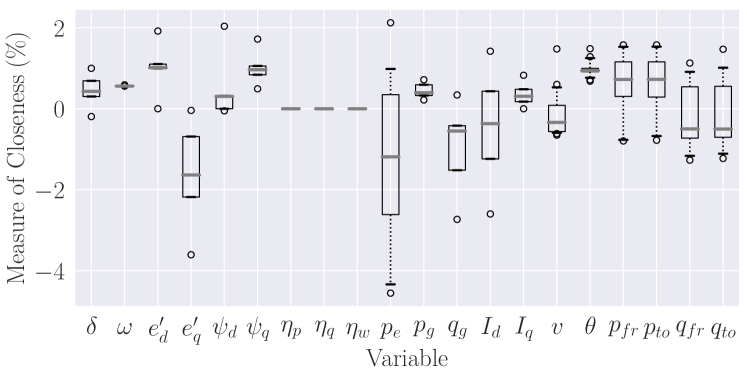
Figure 3: Box plot of the measure of closeness $\epsilon_{\sigma}$ for the IEEE 14-bus system.

Note that, for all the stochastic processes $\eta_{p}$, $\eta_{q}$ and $\eta_{w}$, LEM yields the exact values of $\sigma_{\eta}$. This happens regardless of the process being modeled through either a linear or a non-linear diffusion term. Note also that, to test the accuracy of LEM against the nonlinearity of the SDAEs, we have considered $\sigma(\eta_{p})=\sigma(\eta_{q})$ ranging from $1\%$ to $10\%$ of the initial load consumption. The variations in the values of $\epsilon_{\sigma}$ for all the variables were found to be in the same range as in Fig. 3. It is fair to conclude, thus, that LEM provides very accurate results for a wide range of standard deviation of the stochastic process.

IV-B All-Island Irish Transmission System

This section demonstrates the robustness and light computational burden of the LEM when applied to a real-world complex systems. The model of the AIITS considered in this section consists of 1479 buses, 1851 transmission lines or transformers, 245 loads, 22 conventional synchronous power plants with AVRs and turbine governors, 6 PSSs and 169 wind power plants. Note that the secondary frequency control of the AIITS is implemented manually and, thus, is slower than $200$ s, hence no AGC is considered in the model. Wind speeds are modeled as OU processes. The resulting set of DAEs for the AIITS includes 2278 state variables (666 of which are stochastic processes) and 14623 algebraic variables. The proposed approach was solved for all of the state and algebraic variables but, for space limitation, we can show below only a small selection of these variables.

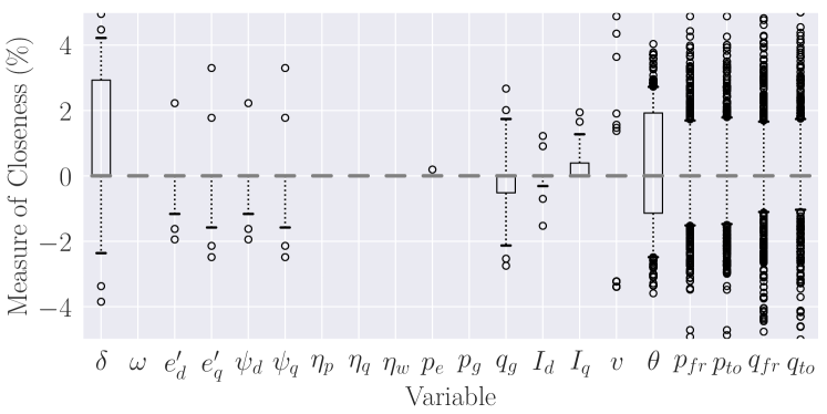
Figure 4: Box plot of the measure of closeness $\epsilon_{\sigma}$ for the AIITS.

The box plot of $\epsilon_{\sigma}$ for the AIITS is shown in Fig. 4. The deviations observed in $\epsilon_{\sigma}$ are of the same order as the $\epsilon_{\sigma}$ observed in IEEE 14-bus system. This result shows that the LEM works for larger systems with the same accuracy as it does for the smaller systems. It is important to note that the solution of (10), which is straightforward per se, depends on the solution of the Lyapunov equation in (9), which is numerically more challenging, especially for large systems. To properly solve (9), the matrix $\boldsymbol{\rm A}_{o}$ has to be well-conditioned to prevent numerical overflow but at the same time to retain the accuracy of the results.

It is also relevant to note that the increase in $\epsilon_{\sigma}$ values does not necessarily need to be interpreted as an error of the proposed approach. Indeed, non-zero values in $\epsilon_{\sigma}$ can be expected in general because $\epsilon_{\sigma}$ is a relative value and none of the two methods (i.e., MC and LEM) is perfect in terms of accuracy. On the one hand, the MC method is a brute-force numerical technique. Its accuracy depends on the number of realizations of the stochastic processes and the time step of the time domain integration, as well as the length of the simulated time. On the other hand, the LEM is analytical and exact, at least for linear or linearized systems. Hence, the deviation between the results obtained with these two techniques is due to (i) the numerical issues of the MC method and (ii) the nonlinearity of the DAEs that model the power system behavior.

LEM shows a clear advantage with respect to MC, at least for large power system models. That is, LEM is characterized by significantly smaller computational times than MC and yields variances of algebraic variables with higher accuracy. In the case of the AIITS, the total CPU time required by MC was $14763$ s, i.e., more than 4 hours, whereas LEM took $12$ s.

V Conclusions

This letter proposes a method to calculate the standard deviation of the algebraic variables of power system modeled as SDAEs. The proposed method is based on the solution of the Lyapunov equation and a linearized method. Simulation results show that the proposed technique has a high accuracy for a wide range of standard deviation of stochastic processes, and significantly reduces the computational time compared to conventional Monte Carlo time domain simulations. Moreover, the proposed method calculates the variance of all algebraic variables based on the knowledge of the variance of the noise sources and the system model, such as load active and reactive power and wind speeds. These are typically known by system operators. The proposed approach appears thus more practical than measuring directly all the algebraic variables in the system. Finally, since the proposed approach is analytical, it makes possible a deeper understanding of the phenomena under study. For example, one can easily and quickly run a sensitivity analysis by varying the elements of $\boldsymbol{\rm G}_{o}$ or design a robust control that minimizes the effect of the noise on certain algebraic variables. These analyses are not straightforward or even possible using the MC method.

The limitations of this method are similar to those of any linearization. We expect that the accuracy of the approach reduces as the time scale of the analysis and, hence, the deviation of the actual system from the linearized model increases. How the accuracy of this approach varies as a function of the time-scale is indeed an open question which we will tackle in future work. In particular, we will also focus on the evaluation of the impact of nonlinearities such as saturations and controller hard limits on the variance of the variables of stochastic power system models as well as on the design of robust controller.

References

- [1] F. Milano and R. Zárate-Miñano, “A systematic method to model power systems as stochastic differential algebraic equations,” IEEE Transactions on Power Systems, vol. 28, no. 4, pp. 4537–4544, 2013.
- [2] H. Xiaoying and P. Kloeden, Random Ordinary Differential Equations and Their Numerical Solution, ser. Probability Theory and Stochastic Modelling. Springer Singapore, 2017, no. 85.
- [3] P. Vorobev, D. M. Greenwood, J. H. Bell, J. W. Bialek, P. C. Taylor, and K. Turitsyn, “Deadbands, droop, and inertia impact on power system frequency distribution,” IEEE Transactions on Power Systems, vol. 34, no. 4, pp. 3098–3108, 2019.
- [4] G. M. Jónsdóttir, M. A. A. Murad, and F. Milano, “On the initialization of transient stability models of power systems with the inclusion of stochastic processes,” IEEE Transactions on Power Systems, vol. 35, no. 5, pp. 4112–4115, 2020.
- [5] G. M. Jónsdóttir and F. Milano, “Data-based continuous wind speed models with arbitrary probability distribution and autocorrelation,” Renewable Energy, vol. 143, pp. 368 – 376, 2019.
- [6] M. Adeen and F. Milano, “Modeling of correlated stochastic processes for the transient stability analysis of power systems,” IEEE Transactions on Power Systems, vol. 36, no. 5, pp. 4445–4456, 2021.
- [7] S. Provost and A. Mathai, Quadratic Forms in Random Variables: Theory and Applications/ A.M. Mathai, Serge B. Provost, ser. Statistics : textbooks and monographs. Marcel Dekker, 1992.
- [8] J. Jacod and P. Protter, Gaussian Random Variables (The Normal and the Multivariate Normal Distributions). Berlin, Heidelberg: Springer Berlin Heidelberg, 2000, pp. 121–135.
- [9] P. Benner, V. Mehrmann, V. Sima, S. Van Huffel, and A. Varga, “SLICOT – A subroutine library in systems and control theory,” in Applied and Computational Control, Signal and Circuits, B. N. Datta, Ed. Birkauser, 1999, vol. 1, ch. 10, pp. 499–539.
- [10] F. Milano, “A Python-based software tool for power system analysis,” in IEEE PES General Meeting, 2013, pp. 1–5.
- [11] R. Zárate-Miñano and F. Milano, “Construction of SDE-based wind speed models with exponentially decaying autocorrelation,” Renewable Energy, vol. 94, pp. 186–196, 2016.
- [12] F. Milano, Power system modelling and scripting. Springer Science & Business Media, 2010.
- [13] M. Adeen and F. Milano, “On the dynamic coupling of the autocorrelation of stochastic processes and the standard deviation of the trajectories of power system variables,” in IEEE PES General Meeting, 2021, pp. 1–5.