Inertia Estimation Through Covariance Matrix

Abstract

This work presents a technique to estimate on-line the inertia of a power system based on ambient measurements. The proposed technique utilizes the covariance matrix of these measurements and solves an optimization problem that fits such measurements to the synchronous machine classical model. We show that the proposed technique is adequate to accurately estimate the actual inertia of synchronous machines and also the virtual inertia provided by the controllers of converter-interfaced generators that emulate the behavior of synchronous machines. We also show that the proposed approach is able to estimate the equivalent damping of the classical synchronous machine model. This feature is exploited to estimate the droop of grid-following converters, which has a similar effect of the swing equation equivalent damping. The technique is comprehensively tested on a modified version of the IEEE 39-bus system as well as on a dynamic 1479-bus model of the all-island Irish transmission system.

I Introduction

I-A Motivation

The inertia constant has become a volatile parameter in power systems with high penetration of renewable and non-synchronous resources [1]. Therefore, the estimation of the available inertia is a valuable information that can help system operators to ensure the security of the grid [2]. This paper addresses this topic and aims at developing an on-line inertia estimation method based on ambient measurements, their stochastic behavior and a fair knowledge of the grid model.

I-B Literature Review

There are mainly two methods for the on-line estimation of the inertia available in a power system: (i) methods based on the measurement of frequency and power variations after a disturbance or by injecting a probing signal and (ii) methods that utilize ambient measurements [3, 4]. Both methods have advantages and shortcomings.

The methods that are based on disturbances can be very accurate [5] provided that the on-set of the disturbance is correctly detected [6, 7, 8, 9]. This can be challenging in low-inertia power systems, which show a “rich” dynamical behavior [10]. Moreover, the estimation cannot be performed continuously, but only following disturbances [11] [12]. Methods based on signal probing must inject active power of adequate magnitude and require the installation of specific equipment or the modification of pre-existing controllers [13].

The methods that utilize ambient measurements are conceptually more challenging than those based on disturbances. The main advantage of these methods is that they employ measurements obtained in normal operating conditions and hence the estimation can be performed in a continuous fashion. The starting point is to build the dynamical model of the system, which can be either complete or reduced to a small number of coherent areas [14, 15]. Then, the values of the parameters and of the observable state variables are fit to available measurements. It is worth mentioning that the number of areas and, consequently, the number of equivalent generators, whose inertia is to be estimated, is relevant. In [16], the authors raise the question whether the center of inertia (coi) of a single-machine-equivalent power system model could be identified through ambient measurements. The answer given is that the combined effects of a well-damped coi dominant mode and of a low-pass-filter action of the Ornstein-Uhlenbeck (ou) processes modelling load behavior make it practically impossible to perform this task. However, this conclusion does not hold when a multi-machine system is considered.

In the latter group of inertia estimation methods, we cite, for example, [17], where the authors obtain the fitting based on a robust Kalman filter. In [13] such a task is performed using a closed-loop identification method. In [18, 19, 20] inertia estimation is performed by observing the step response of the reduced-order model obtained from the full state-space model describing the grid, which is, in turn, obtained through parameter identification using ambient measurements. In [21] the power grid is reduced to a two-machine system and then the system inertia is estimated using inter-area oscillation modes. In [22], the swing equation of the area single-machine-equivalent generator is transformed in Fourier domain. Then, the electromechanical oscillation, obtained by applying a fast Fourier transform to the generator estimated electrical power and rotor speed, are used to estimate the equivalent inertia. This method requires capturing the whole electromechanical oscillation trajectory. The approach proposed in [23] estimates the inertia constants of each generator by applying the regression theorem to a set of ou processes. The method utilizes the covariance and correlation matrices of the state variables to estimate the state matrix of the system. Then, the inertia constants are obtained solving a least-square problem. The main limitation of [23] is the assumption that the relationship between the active power variations of synchronous machines and the voltage angle variations, as well as the active and reactive power variations of converter-interfaced generators are linear. In a similar way, in [24], the regression theorem of a multivariate ou process is applied to power systems including converter-interfaced generators, modeled in detail with their phase locked loops and supposed to work at unity power factor. The estimation is carried out separately for cigs and synchronous generators by identifying the relevant submatrices of the system state matrix.

I-C Contribution

The approach proposed in this work falls in the group of methods that use ambient measurements. We propose to exploit the colored noise due to random fluctuations of the power consumption of the loads and their impact on bus voltages, line currents, and power flows across different areas of a power system. Then we define analytically the statistical properties of the colored noise of these electrical quantities as functions of the system parameters and of the inertia present in the system. Finally, we utilize the variance of the electrical measurements to minimize a non-linear least-squares cost function with respect to the equivalent inertia constants as well as the equivalent damping coefficients of the generators, either synchronous (see, e.g., equation (3.203) in [25]) or power-electronic based, that are connected to the grid. The solution is the sought value of the inertia constant or of the damping coefficient that best fits the measurements and that satisfies the grid constraints.

The main benefit of the proposed approach is that it does not require a contingency or a large disturbance to occur to be able to estimate the inertia (or the damping). Only ambient measurements are needed, together with a fair knowledge of the model of the grid. The price for this is the need to take measurements in a given time period. Nevertheless, as shown in the case studies, the proposed approach is accurate and provides estimations of the inertia in the same time scale of short-term dispatch and adjustments markets. The proposed method is original, as it shows for the first time how to perform inertia estimation by resorting to the covariance matrix of the power system without needing to estimate the state of the network or to derive (or measure) the rotor speed or any other internal variable of both synchronous machines and other devices performing frequency control.

I-D Organization

The remainder of the paper is structured as follows. Section II gives the theoretical mathematical background of power systems’ modeling and in Section III the mathematical model is enriched with the introduction of noise injections to the power system, being this stage instrumental to model load variability and perform the estimation. Section IV presents the proposed estimation procedure. Then the proposed method is validated through numerical simulations, which are discussed in Section V. This section also discusses the challenges posed by the proposed approach and presents a solution based on a proper filtering of the measurements. Finally, conclusions are drawn in Section VI.

II Power System Model

The proposed estimation procedure assumes that the generators connected to the grid are synchronous machines and fits the measurements to this model. In this section, we formulate the equations of the system according to this assumption. It is important to note, however, that every simulation is carried out utilizing a full-fledged model representing in detail the dynamical behavior of all generators, either synchronous or non-synchronous, and their controllers.

To describe the dynamics of the power system model (psm), we consider the following set of differential algebraic equations

$${\boldsymbol{\dot{\delta}}} =\Omega\left(\boldsymbol{\omega}-\omega_{0}\right)\,,$$ (1)

$$\boldsymbol{M}\boldsymbol{\dot{\omega}} =\boldsymbol{P}_{m}(\boldsymbol{\omega},\boldsymbol{x},\boldsymbol{y})-\boldsymbol{P}_{e}(\boldsymbol{\delta},\boldsymbol{x},\boldsymbol{v},\boldsymbol{\theta},\boldsymbol{y})-\boldsymbol{D}(\boldsymbol{\omega}-\omega_{0})$$

$$\boldsymbol{T}\boldsymbol{\dot{x}} =\widehat{\boldsymbol{F}}\left(\boldsymbol{\delta},\boldsymbol{\omega},\boldsymbol{x},\boldsymbol{v},\boldsymbol{\theta},\boldsymbol{y}\right)\,,$$

$$\boldsymbol{0} ={\boldsymbol{G}}\left(\boldsymbol{\delta},\boldsymbol{\omega},\boldsymbol{x},\boldsymbol{v},\boldsymbol{\theta},\boldsymbol{y}\right)~{},$$

where, assuming that $M$ is the number of machines, the meaning of symbols in (1) is as follows:

• $\Omega$: the base synchronous frequency in $\rad/\mathrm{s}$;

• $\boldsymbol{\omega}(t)\in\mathds{R}^{M}$: the per-unit rotor speeds of the machines;

• $\omega_{0}\in\mathds{R}$: the per-unit reference synchronous frequency;

• $\boldsymbol{\delta}(t)\in\mathds{R}^{M}$: the rotor angles of the machines;

• ${\boldsymbol{M}\in\mathds{R}^{M\times M}}$: a diagonal matrix whose entries model the inertia constants ${H}$ of the machines. In particular, $M_{jj}=2H_{jj}$ (for ${j=1,\dots,M}$);

• $\boldsymbol{x}(t)\in\mathds{R}^{N}$: the $N$ state variables of the psm ($\boldsymbol{\omega}$ and $\boldsymbol{\delta}$ excluded) that can influence the dynamics of the machines, and $\boldsymbol{T}\in\mathds{R}^{N\times N}$ is a mass matrix;

• $\boldsymbol{y}(t)\in\mathds{R}^{S}$: all the algebraic variables of the psm but $\boldsymbol{v}$ and $\boldsymbol{\theta}$;

• ${\boldsymbol{D}\in\mathds{R}^{M\times M}}$: a diagonal matrix whose entries $d_{jj}$ (for ${j=1,\dots,M}$) model the damping factor of the machines;

• ${\boldsymbol{v}(t)\in\mathds{R}^{P}}$ and ${\boldsymbol{\theta}(t)\in\mathds{R}^{P}}$: bus voltages and phases, respectively, where $P$ is the number of buses;

• ${\boldsymbol{P}_{m}(\boldsymbol{\omega},\boldsymbol{x},\boldsymbol{y})\in\mathds{R}^{M}}$: the mechanical power regulated by controllers depending on $\boldsymbol{\omega}$, $\boldsymbol{x}$, and $\boldsymbol{y}$;

• $\boldsymbol{P}_{e}(\boldsymbol{\delta},\boldsymbol{x},\boldsymbol{v},\boldsymbol{\theta},\boldsymbol{y})\in\mathds{R}^{M}$: the electrical power exchanged by machines;

• $\widehat{\boldsymbol{F}}(\cdot)$ accounts for regulators and other dynamics included in the system; and

• ${\boldsymbol{G}}(\cdot)$ models algebraic constraints such as lumped models of transmission lines, transformers and static loads.

Equation (1) can be conveniently rewritten as

$$\boldsymbol{\Lambda}\dot{\boldsymbol{\xi}} =\widetilde{\boldsymbol{F}}(\boldsymbol{\xi},\boldsymbol{\zeta})\,,$$ (2)

$$\boldsymbol{0} =\boldsymbol{G}(\boldsymbol{\xi},\boldsymbol{\zeta})~{},$$

where $\displaystyle{\boldsymbol{\xi}(t)\equiv[\boldsymbol{\omega},\boldsymbol{\delta},\boldsymbol{x}]^{\mathrm{T}}}$, $\displaystyle{\boldsymbol{\zeta}(t)\equiv[\boldsymbol{v},\boldsymbol{\theta},\boldsymbol{y}]^{\mathrm{T}}}$, and $\boldsymbol{\Lambda}$ is a non-singular diagonal matrix including $\boldsymbol{M}$. $\boldsymbol{G}$ and $\widetilde{\boldsymbol{F}}$ are assumed to be continuously differentiable in their definition domain and matrices of their partial derivatives are referred to as $\widetilde{\boldsymbol{F}}_{\xi}$, $\widetilde{\boldsymbol{F}}_{\zeta}$, $\boldsymbol{G}_{\xi}$, and $\boldsymbol{G}_{\zeta}$. As an example, $\widetilde{\boldsymbol{F}}_{\xi_{jk}}={\partial\widetilde{\boldsymbol{F}}_{j}}/{\partial\xi_{k}}$, for $j,k=1,...,2M+N$.

The implicit function theorem guarantees that if $\boldsymbol{G}(\boldsymbol{\xi}^{*},\boldsymbol{\zeta}^{*})=\boldsymbol{0}$, provided that $\boldsymbol{G}_{\zeta}(\boldsymbol{\xi}^{*},\boldsymbol{\zeta}^{*})$ is not singular, a unique and smooth function $\boldsymbol{\Gamma}:\mathbb{R}^{2M+N}\rightarrow\mathbb{R}^{2P+S}$ exists so that $\boldsymbol{\zeta}^{*}=\boldsymbol{\Gamma}(\boldsymbol{\xi}^{*})$. If the conditions of the implicit function theorem are satisfied, (2) can be rewritten as

$$\boldsymbol{\Lambda}\dot{\boldsymbol{\xi}} =\widetilde{\boldsymbol{F}}(\boldsymbol{\xi},\boldsymbol{\Gamma}(\boldsymbol{\xi}))\equiv\boldsymbol{F}(\boldsymbol{\xi})~{},$$ (3)

the equilibrium points of which, say $\boldsymbol{\xi}_{o}$, satisfy the condition

$$\boldsymbol{F}(\boldsymbol{\xi}_{o})=\boldsymbol{0}~{},$$ (4)

with the Jacobian matrix

$$\!\boldsymbol{J}(\boldsymbol{\xi}_{o})\!=\!\boldsymbol{\Lambda}^{-1}\!\boldsymbol{F}_{\xi}\!=\!\boldsymbol{\Lambda}^{-1}(\widetilde{\boldsymbol{F}}_{\xi}\!-\!\left.\widetilde{\boldsymbol{F}}_{\zeta}\boldsymbol{G}_{\zeta}^{-1}\!\boldsymbol{G}_{\xi})\right|_{\boldsymbol{\xi}=\boldsymbol{\xi}_{o},\boldsymbol{\zeta}=\boldsymbol{\Gamma}(\boldsymbol{\xi}_{o})}~{}.$$ (5)

III Inclusion of Noise

We assume stochastic noise is injected into the psm as

$$\boldsymbol{\Lambda}\dot{\boldsymbol{\xi}} =\widetilde{\boldsymbol{F}}(\boldsymbol{\xi},\boldsymbol{\zeta})\,,$$ (6)

$$\boldsymbol{0} =\boldsymbol{G}(\boldsymbol{\xi},\boldsymbol{\zeta})+\boldsymbol{\Xi}\,\boldsymbol{\eta}~{},$$

where $\boldsymbol{\eta}$ is a vector of $Z$ independent Ornstein-Uhlenbeck (ou) processes [26], and $\boldsymbol{\Xi}\in\mathbb{R}^{(2P+S)\times Z}$ is a constant matrix.

The ou processes are defined through a set of stochastic differential equations, as follows

$$d\boldsymbol{\eta}=-\boldsymbol{\Upsilon}\boldsymbol{\eta}\,dt+\boldsymbol{\Sigma}\,d\boldsymbol{W}_{t}~{},$$ (7)

where the drift $\boldsymbol{\Upsilon}\in\mathbb{R}^{Z\times Z}$ and diffusion $\boldsymbol{\Sigma}\in\mathbb{R}^{Z\times Z}$ are diagonal matrices with positive entries, $\boldsymbol{W}_{t}\in\mathbb{R}^{Z}$ is a vector of $Z$ Wiener processes, and the differentials rather than time derivatives are utilized to account for the idiosyncrasies of the Wiener processes. The ou processes are characterized by a mean-reversion property and show bound standard deviation. Moreover, these processes show a spectrum that is an accurate model of the stochastic variability of power loads [27, 28, 29, 30, 31]. In (6), we assume that noise injection models the effect of the consumption randomness of $Z$ loads.

Note that, in (6), the vector of stochastic processes $\boldsymbol{\eta}$ appears only in the algebraic equations. This is assumed for simplicity but without lack of generality. The interested reader can find for instance in [29] a stochastic psm model where the noise perturbs both differential and algebraic equations.

We also assume that the action of $\boldsymbol{\eta}$ can be safely modeled as a small-signal perturbation around an equilibrium point. Hence, the solution of (6) can be written as $\boldsymbol{\xi}=\boldsymbol{\xi}_{o}+\boldsymbol{\xi}_{\eta}$ and $\boldsymbol{\zeta}=\boldsymbol{\zeta}_{o}+\boldsymbol{\zeta}_{\eta}$, that is, the effects of perturbations are assumed as additive. It is thus possible to linearise (6) around $\boldsymbol{\xi}_{o}$ and obtain the random ordinary differential equation [32]

$$\boldsymbol{\Lambda}\dot{\boldsymbol{\xi}}_{\eta} =\boldsymbol{F}_{\xi}\boldsymbol{\xi}_{\eta}-\widetilde{\boldsymbol{F}}_{\zeta}\boldsymbol{G}_{\zeta}^{-1}\boldsymbol{\Xi}\,\boldsymbol{\eta}~{},$$ (8)

where the ${\boldsymbol{F}}_{\xi}$, $\widetilde{\boldsymbol{F}}_{\zeta}$, and ${\boldsymbol{G}}_{\zeta}$ matrices are computed at $(\boldsymbol{\xi}_{o},\boldsymbol{\zeta}_{o})$. The small-signal variations of the algebraic variables are given by

$$\boldsymbol{\zeta}_{\eta}=\underbrace{-\boldsymbol{G}_{\zeta}^{-1}\left[\,\boldsymbol{G}_{\xi}|\,\boldsymbol{\Xi}\,\right]}_{\boldsymbol{E}}\left[\!\!\begin{array}[]{c}\boldsymbol{\boldsymbol{\xi}_{\eta}}\\ \boldsymbol{\boldsymbol{\eta}}\end{array}\!\!\right]~{}.$$ (9)

Augmenting (8) with (7) allows obtaining the linear sdes (in narrow sense [26]) governing the overall dynamics of the linearised noisy psm. Adopting the typical formalism of the sdes, the complete set of linearised sdes reads

$$\!d\!\!\underbrace{\left[\!\!\!\begin{array}[]{c}\boldsymbol{\boldsymbol{\xi}_{\eta}}\\ \boldsymbol{\boldsymbol{\eta}}\end{array}\!\!\!\right]}_{\boldsymbol{X}_{t}}\!\!=\!\!\underbrace{\left[\!\!\!\begin{array}[]{cc}\overbrace{\boldsymbol{\Lambda}^{-1}{\boldsymbol{F}}_{\xi}}^{\boldsymbol{J}}\!\!&\!\!-\boldsymbol{\Lambda}^{-1}\widetilde{\boldsymbol{F}}_{\zeta}{\boldsymbol{G}}_{\zeta}^{-1}\boldsymbol{\Xi}\\ \boldsymbol{0}\!\!&\!\!-\boldsymbol{\Upsilon}\end{array}\!\!\!\right]}_{\boldsymbol{A}}\!\!\left[\!\!\!\begin{array}[]{c}\boldsymbol{\boldsymbol{\xi}_{\eta}}\\ \boldsymbol{\boldsymbol{\eta}}\end{array}\!\!\!\right]\!\!dt+\underbrace{\left[\!\!\!\begin{array}[]{c}\boldsymbol{0}\\ \boldsymbol{\Sigma}\end{array}\!\!\!\right]}_{\boldsymbol{B}}\!\!d\boldsymbol{W}_{t}~{},$$ (10)

The solution of (10) with a normally distributed (or constant) initial condition is a $(2M+N+Z)-$dimensional Gaussian stochastic process.

IV Proposed Technique to Estimate the Inertia

The mean and the covariance matrix of process (10) can be derived by solving two sets of linear ordinary differential equations [26]. Since (10) is stable under the hypothesis that (3) is stable at $\boldsymbol{\xi}_{o}$, these odes reveal that, at steady state, the mean of $\boldsymbol{X}_{t}$ is zero, and its $\boldsymbol{K}_{X_{t}}$ covariance matrix derives from the solution of the following Lyapunov equation

$$\boldsymbol{A}\boldsymbol{K}_{X_{t}}+\boldsymbol{K}_{X_{t}}\boldsymbol{A}^{\mathrm{T}}+\boldsymbol{B}\boldsymbol{B}^{\mathrm{T}}=\boldsymbol{0}~{}.$$ (11)

The diagonal elements of $\boldsymbol{K}_{X_{t}}$ are the (steady-state) variances of the components of the $\boldsymbol{X}_{t}$ process. In particular, the last $Z$ diagonal elements, corresponding to the $\boldsymbol{\eta}$ sub-vector of $\boldsymbol{X}_{t}$, are the (steady-state) variances of the $Z$ independent ou processes introduced in (7). Hence, these terms can be written as $\sigma^{2}_{z}/(2\upsilon_{z})$, for $z=1,...,Z$, where $\sigma_{z}$ and $\upsilon_{z}$ are the diagonal elements of $\boldsymbol{\Sigma}$ and $\boldsymbol{\Upsilon}$, respectively [26]. The remaining $2M+N$ diagonal elements of $\boldsymbol{K}_{X_{t}}$ refer to the ${\boldsymbol{\xi}_{\eta}}$ sub-vector of $\boldsymbol{X}_{t}$ and are influenced by $\boldsymbol{\eta}$ through the sub-matrix $-\boldsymbol{\Lambda}^{-1}\widetilde{\boldsymbol{F}}_{\zeta}{\boldsymbol{G}}_{\zeta}^{-1}\boldsymbol{\Xi}$ in (10).

According to (9), $\boldsymbol{\zeta}_{\eta}$ can be written as a linear combination of the entries of $\boldsymbol{X}_{t}$ through $\boldsymbol{E}$, thus being a multidimensional Gaussian process, too. Hence, it is possible to write the $\boldsymbol{K}_{\zeta_{\eta}}$ covariance matrix of the small-signal algebraic variables as the quadratic form [33, 34]

$$\boldsymbol{K}_{\zeta_{\eta}}=\boldsymbol{E}\boldsymbol{K}_{X_{t}}\boldsymbol{E}^{\mathrm{T}}~{}.$$ (12)

The proposed approach exploits (12) and the fact that $\boldsymbol{K}_{\zeta_{\eta}}$ (and, thus, the variance of the algebraic variables) depends through $\boldsymbol{K}_{X_{t}}$ and $\boldsymbol{A}$ on the elements of $\boldsymbol{\Lambda}$, a subset of which are the inertia constants of the synchronous machines.

Let us assume one wants to estimate a subset $\mathcal{M}$ of these inertia constants and let $\mathcal{Z}$ be a set of pmu measurements of bus voltages and line currents flowing through a given number of transmission lines and/or transformers.

The above derivations show that, if the model and the parameters of the grid are known, one can compute the $\sigma^{2}_{\mathcal{Z}}$ variances of the measured quantities, which are the diagonal elements of the $\boldsymbol{K}_{\zeta_{\eta}}$ matrix. However, it is also possible to solve an inverse problem: knowing through measurements the variance of the elements of $\mathcal{Z}$, the values of the elements of $\mathcal{M}$ can be determined by minimizing the following non-linear least-squares cost function (see also Fig. 1)

$$\left.\mathcal{C}(\mathcal{M})\right|_{\widetilde{\boldsymbol{F}}_{\xi},\widetilde{\boldsymbol{F}}_{\zeta},{\boldsymbol{G}}_{\xi},{\boldsymbol{G}}_{\zeta}}=\sum_{\mathcal{Z}}{\frac{(\widehat{\sigma}^{2}_{\mathcal{Z}}-\sigma^{2}_{\mathcal{Z}}(\mathcal{M}))^{2}}{\sigma^{4}_{\mathcal{Z}}(\mathcal{M}^{*})}}~{},$$ (13)

where $\widehat{\sigma}^{2}_{\mathcal{Z}}$ are the variances of the measured variables, $\sigma^{2}_{\mathcal{Z}}(\mathcal{M})$ are the variances computed in run-time during the minimization procedure w.r.t. the elements of $\mathcal{M}$, while $\sigma^{2}_{\mathcal{Z}}(\mathcal{M}^{*})$ are the corresponding variances of the same variables obtained with the model for a reference set of $\mathcal{M}$ values, which are used to normalize the cost function.

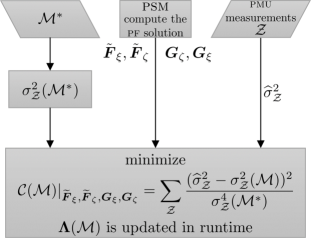
Figure 1: The flow-diagram of the proposed inertia estimation procedure.

During the optimization process the estimation of the elements of $\mathcal{M}$ makes necessary to update, iteratively, $\boldsymbol{\Lambda}$ and, consequently, $\boldsymbol{A}$.

We note that the procedure above is agnostic w.r.t. to the devices that are connected to the grid. That is, the estimation of the inertia is obtained by fitting the synchronous machine model to the measurements. If there exist non-synchronous devices, such as converter-interfaced generation, their “equivalent” inertia constants can be obtained using (13) regardless of the fact that the converter is set up to be grid forming or grid following. The procedure is also agnostic in terms of the parameters to be estimated, provided that such parameters do have an effect on the frequency variations of the system. In particular, we use this property to estimate also the equivalent damping coefficients of the devices, which can be attained by minimizing a cost function for a subset of damping coefficients $\mathcal{D}$, in a similar way as for $\mathcal{M}$ in (13),

$$\left.\mathcal{C}(\mathcal{D})\right|_{\widetilde{\boldsymbol{F}}_{\xi},\widetilde{\boldsymbol{F}}_{\zeta},{\boldsymbol{G}}_{\xi},{\boldsymbol{G}}_{\zeta}}=\sum_{\mathcal{Z}}{\frac{(\widehat{\sigma}^{2}_{\mathcal{Z}}-\sigma^{2}_{\mathcal{Z}}(\mathcal{D}))^{2}}{\sigma^{4}_{\mathcal{Z}}(\mathcal{D}^{*})}}~{}.$$ (14)

V Case Studies

In this Section, we consider two grids, the well known IEEE 39-bus system and a 1479-bus dynamic model of the all-island Irish transmission system aiits. The IEEE 39-bus system allows us illustrating the various features and challenges of the proposed method. With this aim we first consider the conventional system with synchronous machines and their regulators (Section V-A1). Then, we evaluate the behavior of the proposed method when the system includes grid-forming (Section V-A2) and grid-following converters (Section V-A3). The all-island Irish system, on the other hand, serves to demonstrate the robustness of the proposed method when applied to a real-world complex network.

V-A IEEE 39-bus System

We use as a benchmark the IEEE 39-bus power system shown in Fig. 2 [35]. This is a simplified model of the transmission system in the New England region in the Northeastern United States and is composed of $10$ generators, $34$ lines, $19$ loads, and $12$ transformers. The network models and parameters are those adopted and directly extracted from its DIgSILENT PowerFactory implementation [36] and derived from [37]. The $G_{1}$ generator, which represents the connection of the New England System to the rest of the US and Canadian grid, is modeled with a constant excitation [37], viz. there is no automatic voltage regulator (avr) connected to it. On the contrary, the other generators are equipped with avrs (specifically, rotating excitation systems of IEEE Type 1 according to [37]). Governors are considered as IEEE Type G1 (steam turbine) for $G_{2}$–$G_{9}$, and IEEE Type G3 (hydro turbine) for $G_{10}$. Finally, in Table I we report the value of inertia constants and power rating of the 10 generators.

Figure 2: The single-line diagram of the IEEE 39-bus power system.

TABLE I: Synchronous generators $H$ and $P_{\mathrm{RAT}}$

Gen.	$H\,[\mathrm{s}]$	$P_{\mathrm{RAT}}\,[\mathrm{M}\mathrm{W}]$	Gen.	$H\,[\mathrm{s}]$	$P_{\mathrm{RAT}}\,[\mathrm{M}\mathrm{W}]$
$G_{1}$	$5.00$	$10000$	$G_{6}$	$4.35$	$800$
$G_{2}$	$4.33$	$700$	$G_{7}$	$3.77$	$700$
$G_{3}$	$4.47$	$800$	$G_{8}$	$3.47$	$700$
$G_{4}$	$3.57$	$800$	$G_{9}$	$3.45$	$1000$
$G_{5}$	$4.33$	$600$	$G_{10}$	$4.20$	$1000$

The active power consumption of each of the $Z=19$ loads is altered by one of the $\eta_{z}(t)$ ou processes ($z=1,\dots,Z$) in (10), which has zero mean, and variance $\sigma_{z}^{2}/(2\upsilon_{z})$. All loads are assumed to incorporate stochastic power fluctuations [29]

$$\mathrm{L}_{z}(t)=\eta_{z}(t)\,P_{{\mathrm{L0}}_{z}}\left(\frac{\left|V_{z}(t)\right|}{V_{0_{z}}}\right)^{\gamma}~{},$$ (15)

where (for $z=1,\dots,Z$) $P_{{\mathrm{L0}}_{z}}$ is the nominal active power of the load, $V_{0_{z}}$ is the load voltage rating, $V_{z}(t)$ is the bus voltage at which the load is connected and $\gamma$ governs the dependence of the load on bus voltage. In the simulation below, we assume $\upsilon_{z}=0.5$ and $\sigma_{z}$ is defined in such a way that the standard deviation of $\eta_{z}(t)$ is $5\%$ of $P_{\mathrm{L0}}$. The zero mean implies that stochastic load power fluctuations do not perturb, on average, the operating point of the system. Furthermore, we assumed $\gamma=0$.

To carry out the simulations discussed below, the numerical integration of the multi-dimensional ou process in (6) was based on the numerical scheme proposed by Gillespie in [38]. Furthermore, the second-order trapezoidal implicit weak scheme for stochastic differential equations with colored noise, available in the simulator pan [39, 40, 41], was adopted [42].

V-A1 Conventional Power System

The objective of the first scenario considered in this case study is to estimate the inertia constants of the 10 generators of the IEEE 39-bus system across a time period spanning one day. The target is to obtain an estimation of the inertia constants every $15\,\mathrm{min}$ (estimation window) of the working day. To this end, we compute the variance of the currents flowing through the generators, using a $15\,\mathrm{min}$-long moving window. The values of variance are the elements of the $\mathcal{M}$ set introduced in Sec. IV. The sampling period is $25\,\mathrm{m}\mathrm{s}$, i.e., a sampling rate of $40\,\mathrm{Hz}$.

We also assume that the matrices $\tilde{\boldsymbol{F}}_{\boldsymbol{\xi}}$, $\tilde{\boldsymbol{F}}_{\boldsymbol{\zeta}}$, ${\boldsymbol{G}}_{\boldsymbol{\xi}}$, ${\boldsymbol{G}}_{\boldsymbol{\zeta}}$ are constant, i.e., that the parameters of the IEEE 39-bus system do not vary during the simulation. This assumption simplifies the analysis but is not a binding requirement of the proposed procedure. If the operating point and/or the topology of the grid change, one just needs to update those matrices.

The $\widehat{H}$ inertia constant estimates were obtained with the MATLAB Global Optimization Toolbox and the fgoalattain function. The search interval of the optimization procedure was lower-bounded to zero since inertia constants cannot be negative. We performed $20$ independent trials each one being a $24\,\mathrm{h}$ simulation of the grid and an optimization problem is solved every $15\,\mathrm{min}$ of simulated time, thus collecting $1920$ estimates per synchronous generator. The violin plots in Fig. 3 (one for each generator) summarize the obtained results. The median of the estimated value of the inertia constants (black solid dots in Fig. 3) are in good agreement with the corresponding nominal values (empty squared markers in Fig. 3) listed in Table I. Despite the amplitude of the interquartile range (iqr) intervals (magenta vertical bars in Fig. 3) are reasonably narrow, the upper and lower adjacent values (green solid dots in Fig. 3) are quite far from the median values, and the same holds for the tails of the distribution of the estimated values. The maximum value of the relative percentage error, computed as $\epsilon_{\%}^{H}=100\cdot\frac{|\text{Median}(\widehat{H})-H|}{H}$, is obtained for $G_{5}$ and amounts to $3.87\%$. The $0.44\%$ minimum value is achieved for $G_{3}$.

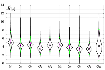
Figure 3: Violin plots of the inertia estimations of each generator of the IEEE 39-bus system. The black solid circle markers correspond to the median value of the optimization results, whereas the empty square markers represent the nominal values of the inertia constants. The magenta bars represent the iqr, viz. the spread difference between the $75^{\mathrm{th}}$ and $25^{\mathrm{th}}$ percentiles of the data. The green solid circle markers represent the upper adjacent value (i.e., the largest observation that is less than or equal to the third quartile plus $1.5\times\acs{iqr}$) and the lower adjacent value (i.e., the smallest observation that is greater than or equal to the first quartile minus $1.5\times\acs{iqr}$). Time window: $15$ min. Optimization performed on the unfiltered currents.

The quality of the results can be improved by filtering the considered currents before computing their moving variance. This is done by resorting to a steep bandpass filter acting from $0.1\,\mathrm{Hz}$ to $1.5\,\mathrm{Hz}$. This bandwidth was chosen to remove the low frequency contribution of the ou process. This is done since these components account for the very slow fluctuations of the currents that heavily affect the trend of their moving variance w.r.t. the steady-state values of the variance itself. The effect of this filter is shown in Fig. 4 for the $i_{8}$ current (i.e., the current flowing through $G_{8}$) in terms of the absolute value of the relative percentage error between the moving variance and its steady-state value over $24\,\mathrm{h}$ in one of the $20$ trials. In particular, the black and red curves refer to the unfiltered and the filtered case, respectively, and the improvement over the unfiltered case is evident.

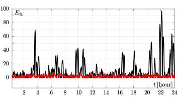
Figure 4: The $E_{\%}$ percentage relative error of the moving variance of the $i_{8}$ current, calculated over a sliding window of $15\,\mathrm{min}$, with respect to the steady-state variance of $i_{8}$. The black and the red curves refer to the unfiltered and filtered case, respectively.

The state equations governing the dynamics of the filters were added to the set of odes reported in (3) and this allowed to derive the steady-state variance of the filters output solving (11). The inertia constants of the IEEE 39-bus generators was estimated from the filtered currents and the results are reported in Fig. 5. The effect of this signal processing is a significant reduction of the amplitude of the interval spanned by the upper and lower adjacent values, thus guaranteeing a more reliable estimate of the inertia constants. The $\epsilon_{\%}^{H}$ relative percentage error spans from $0.14\%$ (for $G_{2}$) to $1.78\%$ (for $G_{9}$). These results illustrate well that the proposed approach accurately estimates the inertia constants of the ten synchronous generators of the system.

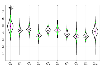
Figure 5: Violin plots of the inertia estimations of each generator of the IEEE 39-bus system. The optimization was performed on the filtered currents, on a time window of $15\,\mathrm{min}$. Note the different scale of the vertical axes w.r.t. Fig. 3.

V-A2 Inclusion of Grid-Forming Converters

This section illustrates the behavior of the proposed estimation technique for a scenario where the IEEE 39-bus system is modified to include a variable generation/load profile and grid-forming converters. These devices are assumed to mimic the behavior of synchronous machines and are thus expected to provide a virtual inertia to the system. The controllers of grid-forming converters are based on [43]. The objective of this section is twofold: (i) showing that the proposed inertia estimation approach works correctly under variable generation/load conditions and (ii) illustrating the ability of the proposed estimation technique to capture the effect of grid-forming converters.

For what regards point (i), we first modified the IEEE 39-bus system by mimicking a typical daily variation of the loads. To do so, we multiplied the power absorbed by the loads and the (active) power generated by the synchronous machines by a coefficient $\lambda$. To alter the nominal value of the power loads, $\lambda$ was varied continuously in time according to the profile shown in the upper panel of Fig. 6. This profile was sampled every $15\,\mathrm{min}$: this same time basis was used to update the set points of the generators. The effect of energy production by three (aggregated) solar plants connected to $\tt{bus_{8}}$, $\tt{bus_{24}}$, and $\tt{bus_{27}}$ was emulated by reducing the absorbed active power of the loads connected at those buses. Load power was decreased by the same active power supplied by those (aggregated) solar plants (each one supplying one third of the electrical power reported in the lower panel of Fig. 6). To balance generation, the power supplied by these plants was subtracted from the power of synchronous generators. In particular, the active power supplied by $G_{3}$, $G_{7}$, and $G_{8}$ was varied in proportion to their power ratings. Concerning point (ii), the power rating of each one of the virtual synchronous generators (i.e., the solar plants connected to $\tt{bus_{8}}$, $\tt{bus_{24}}$, and $\tt{bus_{27}}$) is $100\,\mathrm{M}\mathrm{W}$. We regulated these generators so that each of them provided, through the controllers of their inverters, a total virtual inertia equivalent to $H=10\,\mathrm{s}$ only from 8:15  to 5:30 .

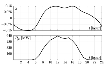
Figure 6: Upper panel: time evolution of the $\lambda$ coefficient used to overload the IEEE 39-bus system. Lower panel: the overall active power supplied by the solar plants that were added to the IEEE 39-bus system.

Results are shown in Fig. 7, using again violin plots. The left panel refers to the time interval in which the solar plants are not connected and thus the inertia constants of their grid-forming converters is zero. The right panel corresponds to the 8:15  – 5:30  time interval. In the high-inertia case, the $\epsilon_{\%}^{H}$ percentage error for $\rm GFM_{1}$, $\rm GFM_{2}$, and $\rm GFM_{3}$ is equal to $0.29\%$, $1.23\%$, and $0.60\%$, respectively. In the low-inertia case, $\epsilon_{\%}^{H}$ is almost the same for the three grid-forming converters and amounts to $0.02\%$.

The estimation is accurate even though we used only the measurements of the current flowing through the lines connecting $\tt{bus_{1}-bus_{39}}$, $\tt{bus_{9}-bus_{39}}$, $\tt{bus_{3}-bus_{4}}$, $\tt{bus_{16}-bus_{17}}$, and $\tt{bus_{14}-bus_{15}}$, (i.e., the branches indicated with dashed lines in Fig. 2), which are far away from the buses connecting the solar power plants. As reported in the literature, these lines split the IEEE 39-bus system in areas.

The measurements used in this case highlight that we do not necessarily need to put pmus in front of synchronous generators or grid-forming/following converters. However, we do not have a systematic method that clearly indicates the optimal locations where pmus should be connected to provide measurements used during the estimation process. This is an open issue that we will cope with in future work.

Moreover, we observe the birth of additional “swing equation” modes due to the presence of this kind of the virtual synchronous generators [44]. These, in fact, induce inter-area oscillations that are clearly identified by peaks in the frequency responses by frequency scan. Modifying the inertia constant of these elements changes significantly the variance of the measured electrical quantities and, thus, helps increasing the accuracy of the proposed technique.

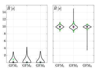
Figure 7: Violin plots of the inertia constants estimates of the grid-forming converters $\rm GFM_{1}$, $\rm GFM_{2}$, and $\rm GFM_{3}$ (all of which were set to $10\,\mathrm{s}$ from 8:15  to 5:30 ). Left and right panels refer to the low- and high-inertia cases, respectively. The time window is $15\,\mathrm{min}$.

Figure 8 shows the estimation of the inertia of the system across the full day of measurements. This illustrates the effectiveness of the proposed technique to continuously estimate the inertia by stochastic fluctuations. In Fig. 8, the black traces are single trials while the red one is the median value over $50$ trials. All realisations give accurate results with only a few time instants being affected by a relatively higher error.

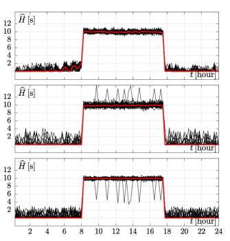
Figure 8: From top to bottom: inertia constant estimates over time of the grid-forming converters $\rm GFM_{1}$, $\rm GFM_{2}$, and $\rm GFM_{3}$ (all of which were set to $10\,\mathrm{s}$ from 8:15  to 5:30 ). The results of the $50$ estimation procedures are depicted in black. In red we report the median value computed every $15\,\mathrm{min}$ over the $50$ trials.

V-A3 Inclusion of Grid-Following (GFL) Converters

In the third and last scenario, we discuss the effect of the frequency droop control of grid-following converters on the estimation of the inertia with the proposed technique. As is well-known, the frequency droop control of the converter is equivalent to a second order model, and is thus similar to that of synchronous machines, except for the fact that it shows a large damping and approximately zero inertia [45]. In this scenario, thus, we repeat the simulations of the modified IEEE 39-bus system with inclusion of the same solar power plants considered in the previous section. However, we assume that these plants are now equipped with conventional frequency droop controllers.

Table II shows that the estimation of the damping/droop and of the inertia are strongly correlated. An increase in the droop coefficients of the frequency controllers leads to a lower inertia constant estimation. This result had to be expected as a lower droop makes the response of the controller slower and thus its time scale tends to overlap with that of the inertial response. The estimation of the inertia constant and of the damping coefficient are performed independently, since two separate least-squares problems are solved: one fits the inertia constant and a second one fits the damping coefficient.

The main conclusion that can be drawn from the results shown in Table II is that the value of the inertia constant alone is not sufficient to define the ability of a device to regulate the frequency. If only the inertia constant is estimated, in fact, one would conclude that the case with higher droop coefficient is the one with lower frequency containment, which is not. On the other hand, if both parameters, namely inertia and damping, are estimated, then one can conclude, correctly, that the system with higher droop provides “more” fast frequency control than inertial response. On the other hand, lower droop values increase the ability of the system to have an inertial response but lead, as expected, to a lower capability of providing a service as fast frequency controllers.

TABLE II: Estimation of the equivalent inertia and of the damping/droop for the grid-following converters in the modified IEEE 39-bus system.

Device	$\text{droop}=2$		$\text{droop}=10$
	$H_{eq}$ [$\mathrm{s}$]	$D_{eq}$ [$\mathrm{pu}$]	$H_{eq}$ [$\mathrm{s}$]	$D_{eq}$ [$\mathrm{pu}$]
$\rm GFL_{1}$	0.64	3.29	0.40	8.65
$\rm GFL_{2}$	0.60	3.13	0.37	7.97
$\rm GFL_{3}$	0.56	3.93	0.34	10.57

V-B All-Island Irish Transmission System (aiits)

In this section, the proposed method is applied to a real-world complex system. The model of the aiits considered here consists of 1479 buses, 1851 transmission lines or transformers, 245 loads, 22 conventional synchronous power plants with avrs and turbine governors, 6 power system stabilizers, and 169 wind power plants. Note that the secondary frequency control of the aiits is implemented manually and, thus, no agc is considered in the model. Both load fluctuations and wind speeds are modeled as ou processes. The resulting set of DAEs for the aiits includes 2118 state variables (663 of which are stochastic processes) and 6175 algebraic variables. Both the active and the reactive power of the $Z=245$ loads is altered by an ou process characterised by $v=0.1$, while $\sigma$ is defined in such a way that the standard deviation of those processes is $0.5\%$ of the nominal active or reactive power of each load. Finally, the standard deviation and drift term of the ou processes modeling the wind speeds are set to $0.002$ and $0.02$, respectively. The time domain simulations of the aiits are obtained with the software tool Dome [46].

To test the applicability of the proposed method, we estimated the $\widehat{H}$ inertia constants of $11$ conventional synchronous power plants chosen to be representative of non-homogeneous $H$ constants and power ratings (see Table III). An optimization problem was solved every $15\,\mathrm{min}$ of simulated time by collecting $100$ estimates per synchronous generator. Making reference to the diagram in Figure 1, the subset $\mathcal{Z}$ contains only the magnitude of the voltage at the buses where the generators are connected. Hence we did not resort to the phase of such voltages, to any current of the network, or to any rotor speed of the synchronous generators.

The $\epsilon_{\%}^{H}$ relative percentage error spans from $0.22\%$ (for $G_{7}$) to $5.42\%$ (for $G_{10}$). The quality of the results, measured through $\epsilon_{\%}^{H}$, is similar to that obtained for the IEEE 39-bus system. For the sake of readability, the violin plots in Fig. 9 report the statistics of the $\widehat{H}$ estimated inertia values normalized w.r.t. the $H$ nominal inertia of each generator. So doing, for each violin plot in Fig. 9 the reference value is $1$. The distance of the upper and lower adjacent values (green solid dots in Figure 9) from the expected normalized value of $\widehat{H}$ is lower than $0.22$ for all the $11$ synchronous generators, which confirms the robusteness of the proposed method when applied to a real-world complex system with several hundreds of buses and dynamic devices.

TABLE III: Synchronous generators $H$ and $P_{\mathrm{RAT}}$ of the aiits

Gen.	$H\,[\mathrm{s}]$	$P_{\mathrm{RAT}}\,[\mathrm{M}\mathrm{W}]$	Gen.	$H\,[\mathrm{s}]$	$P_{\mathrm{RAT}}\,[\mathrm{M}\mathrm{W}]$
$G_{1}$	$15.924$	$535.5$	$G_{7}$	$10.000$	$135$
$G_{2}$	$13.400$	$288$	$G_{8}$	$11.652$	$292$
$G_{3}$	$7.320$	$87.5$	$G_{9}$	$7.744$	$353$
$G_{4}$	$7.320$	$87.5$	$G_{10}$	$7.744$	$127.6$
$G_{5}$	$7.320$	$87.5$	$G_{11}$	$10.700$	$359$
$G_{6}$	$14.344$	$22.47$

Figure 9: Violin plots of the inertia constants estimates for some generators of the aiits, normalized w.r.t. their effective value.

VI Conclusions

This work proposes a technique to estimate the inertia based on the variance of measurements. Assuming a given model of the power system and the dynamics of the generators, the technique fits this model to the measurements by solving a least-squares problem. Simulation results show that the proposed technique, given an adequate filtering of the measurements, is accurate even in a real-world complex system and can take into account both conventional and virtual synchronous machines, as well as the effect of frequency droop controllers. However, the correct interpretation of the effect of droop controllers is consistent only if also the damping/droop coefficients are estimated, which the proposed technique duly allows to obtain.

In particular, we believe that the proposed technique can be useful to reward the frequency support provided by non-synchronous devices. In turn, we recommend that the reward should be evaluated based on the effect that the controllers of these devices have on the system, not on the actual implementation of the control itself.

Future work will focus on further investigating the theoretical and practical aspects of the proposed technique. For example, relevant questions are how to improve the accuracy of the estimated inertia constants through (i) an optimal number and location of the set of measurements and (ii) of the filtering of the measurements.

Federico Bizzarri (M’12–SM’14) was born in Genoa, Italy, in 1974. He received the Laurea (M.Sc.) five-year degree (summa cum laude) in electronic engineering and the Ph.D. degree in electrical engineering from the University of Genoa, Genoa, Italy, in 1998 and 2001, respectively. Since October 2018 he has been an associate professor at the Electronic and Information Department of the Politecnico di Milano, Milan, Italy. He is a research fellow of the Advanced Research Center on Electronic Systems for Information and Communication Technologies “E. De Castro” (ARCES), University of Bologna, Italy. He served as an Associate Editor of the IEEE Transactions on Circuits and Systems — Part I from 2012 to 2015 and he was awarded as one of the 2012-2013 Best Associate Editors of this journal.

Davide del Giudice was born in Milan, Italy, in 1993. He received the M.S. degree and the Ph.D. degree in electrical engineering from Polytechnic of Milan in 2017 and 2022, respectively. He is currently a researcher at the department of Electronics, Information and Bioengineering of Polytechnic of Milan. His main research activities are related to simulation techniques for electric power systems with a high penetration of converter-interfaced elements, such as high voltage direct current systems, electric vehicles and generation fuelled by renewables.

Samuele Grillo (S’05–M’09–SM’15) received the Laurea degree in electronic engineering, and the Ph.D. degree in power systems from the University of Genova, Italy, in 2004 and 2008, respectively. He is currently an Associate Professor with the Dipartimento di Elettronica, Informazione e Bioingegneria, Politecnico di Milano, Milan, Italy. Since 2018 he is a contributor to CIGRÉ Working Group B5.65 “Enhancing Protection System Performance by Optimising the Response of Inverter-Based Sources.” His research interests include smart grids, integration of distributed renewable sources, and energy storage devices in power networks, optimization, and control techniques applied to power systems.

Daniele Linaro Daniele Linaro received his MSc in Electronic Engineering from the University of Genoa (Italy) in 2007 and a PhD in Electrical Engineering from the same university in 2011. Since 2018, he is Assistant Professor in the Department of Electronics, Information Technology and Bioengineering at the Polytechnic of Milan. His main research interests are currently in the area of circuit theory and nonlinear dynamical systems, with applications to electronic oscillators and power systems and computational neuroscience, in particular biophysically-realistic single-cell models of neuronal cells.

Angelo Brambilla (M’16) received the Dr. Ing. degree in electronics engineering from the University of Pavia, Pavia, Italy, in 1986. He is full professor at the Dipartimento di Elettronica, Informazione e Bioingegneria, Politecnico di Milano, Milano, Italy, where he has been working in the areas of circuit analysis, simulation and modeling.

Federico Milano (F’16) received from the Univ. of Genoa, Italy, the ME and Ph.D. in Electrical Eng. in 1999 and 2003, respectively. From 2001 to 2002 he was with the Univ. of Waterloo, Canada, as a Visiting Scholar. From 2003 to 2013, he was with the Univ. of Castilla-La Mancha, Spain. In 2013, he joined the Univ. College Dublin, Ireland, where he is currently Prof. of Power Systems Control and Protections and Head of Elec. Eng. In 2022, he was appointed Co-Editor in Chief of the IET Generation Transmission & Distribution. His research interests include power system modeling, control and stability analysis.

References

- [1] A. Ulbig, T. S. Borsche, and G. Andersson, “Impact of low rotational inertia on power system stability and operation,” IFAC Proceedings Volumes, vol. 47, no. 3, pp. 7290–7297, 2014, 19th IFAC World Congress. [Online]. Available: https://www.sciencedirect.com/science/article/pii/S1474667016427618
- [2] F. Milano, F. Dörfler, G. Hug, D. J. Hill, and G. Verbič, “Foundations and challenges of low-inertia systems (invited paper),” in 2018 Power Systems Computation Conference (PSCC), 2018, pp. 1–25.
- [3] B. Tan, J. Zhao, M. Netto, V. Krishnan, V. Terzija, and Y. Zhang, “Power system inertia estimation: Review of methods and the impacts of converter-interfaced generations,” Int. J. Electr. Power Energy Syst., vol. 134, no. 107362, 2022.
- [4] S. C. Dimoulias, E. O. Kontis, and G. K. Papagiannis, “Inertia Estimation of Synchronous Devices: Review of Available Techniques and Comparative Assessment of Conventional Measurement-Based Approaches,” Energies, vol. 15, no. 20, pp. 1–30, 2022.
- [5] U. Tamrakar, N. Guruwacharya, N. Bhujel, F. Wilches-Bernal, T. M. Hansen, and R. Tonkoski, “Inertia estimation in power systems using energy storage and system identification techniques,” in 2020 International Symposium on Power Electronics, Electrical Drives, Automation and Motion (SPEEDAM), 2020, pp. 577–582.
- [6] P. Wall and V. Terzija, “Simultaneous Estimation of the Time of Disturbance and Inertia in Power Systems,” IEEE Trans. Power Del., vol. 29, no. 4, pp. 2018–2031, Aug. 2014.
- [7] D. Zografos, M. Ghandhari, and R. Eriksson, “Power system inertia estimation: Utilization of frequency and voltage response after a disturbance,” Electr. Pow. Syst. Res., vol. 161, pp. 52–60, 2018.
- [8] P. M. Ashton, C. S. Saunders, G. A. Taylor, A. M. Carter, and M. E. Bradley, “Inertia Estimation of the GB Power System Using Synchrophasor Measurements,” IEEE Trans. Power Syst., vol. 30, no. 2, pp. 701–709, Mar. 2015.
- [9] D. del Giudice and S. Grillo, “Analysis of the Sensitivity of Extended Kalman Filter-Based Inertia Estimation Method to the Assumed Time of Disturbance,” Energies, vol. 12, no. 483, 2019.
- [10] E. Heylen, F. Teng, and G. Strbac, “Challenges and opportunities of inertia estimation and forecasting in low-inertia power systems,” Renew. Sustain. Energy Rev., vol. 147, no. 111176, 2021.
- [11] R. K. Panda, A. Mohapatra, and S. C. Srivastava, “Online Estimation of System Inertia in a Power Network Utilizing Synchrophasor Measurements,” IEEE Trans. Power Syst., vol. 35, no. 4, pp. 3122–3132, Jul. 2020.
- [12] G. Cai, B. Wang, D. Yang, Z. Sun, and L. Wang, “Inertia Estimation Based on Observed Electromechanical Oscillation Response for Power Systems,” IEEE Trans. Power Syst., vol. 34, no. 6, pp. 4291–4299, Nov. 2019.
- [13] J. Zhang and H. Xu, “Online Identification of Power System Equivalent Inertia Constant,” IEEE Trans. Ind. Electron., vol. 64, no. 10, pp. 8098–8107, Oct. 2017.
- [14] G. R. Moraes, F. Pozzi, V. Ilea, A. Berizzi, E. M. Carlini, G. Giannuzzi, and R. Zaottini, “Measurement-based inertia estimation method considering system reduction strategies and dynamic equivalents,” in 2019 IEEE Milan PowerTech, 2019, pp. 1–6.
- [15] K. Tuttelberg, J. Kilter, D. Wilson, and K. Uhlen, “Estimation of Power System Inertia From Ambient Wide Area Measurements,” IEEE Trans. Power Syst., vol. 33, no. 6, pp. 7249–7257, Nov. 2018.
- [16] A. Gorbunov, J. C.-H. Peng, J. W. Bialek, and P. Vorobev, “Can Center-of-Inertia Model be Identified From Ambient Frequency Measurements?” IEEE Trans. Power Syst., vol. 37, no. 3, pp. 2459–2462, 2022.
- [17] J. Zhao, Y. Tang, and V. Terzija, “Robust Online Estimation of Power System Center of Inertia Frequency,” IEEE Trans. Power Syst., vol. 34, no. 1, pp. 821–825, Jan. 2019.
- [18] F. Zeng, J. Zhang, G. Chen, Z. Wu, S. Huang, and Y. Liang, “Online estimation of power system inertia constant under normal operating conditions,” IEEE Access, vol. 8, pp. 101 426–101 436, 2020.
- [19] V. Baruzzi, M. Lodi, A. Oliveri, and M. Storace, “Analysis and improvement of an algorithm for the online inertia estimation in power grids with RES,” in 2021 IEEE International Symposium on Circuits and Systems (ISCAS). IEEE, 2021, pp. 1–5.
- [20] ——, “Estimation of inertia in power grids with turbine governors,” in 2022 IEEE International Symposium on Circuits and Systems (ISCAS). IEEE, 2022, pp. 1–5.
- [21] D. Yang, B. Wang, J. Ma, Z. Chen, G. Cai, Z. Sun, and L. Wang, “Ambient-data-driven modal-identification-based approach to estimate the inertia of an interconnected power system,” IEEE Access, vol. 8, pp. 118 799–118 807, 2020.
- [22] B. Wang, D. Yang, G. Cai, Z. Chen, and J. Ma, “An Improved Electromechanical Oscillation-Based Inertia Estimation Method,” IEEE Trans. Power Syst., vol. 37, no. 3, pp. 2479–2482, May 2022.
- [23] J. Guo, X. Wang, and B.-T. Ooi, “Online purely data-driven estimation of inertia and center-of-inertia frequency for power systems with vsc-interfaced energy sources,” Int. J. Electr. Power Energy Syst., vol. 137, no. 107643, 2022.
- [24] ——, “Estimation of Inertia for Synchronous and Non-Synchronous Generators Based on Ambient Measurements,” IEEE Trans. Power Syst., vol. 37, no. 5, pp. 3747–3757, Sep. 2022.
- [25] P. Kundur, Power system stability and control. New York: McGraw-Hill, 1994.
- [26] L. Arnold, Stochastic differential equations, ser. A Wiley-Interscience publication. Wiley, 1974.
- [27] R. H. Hirpara and S. N. Sharma, “An Ornstein-Uhlenbeck process-driven power system dynamics,” IFAC-PapersOnLine, vol. 48, no. 30, pp. 409–414, 2015, 9th IFAC Symposium on Control of Power and Energy Systems CPES 2015.
- [28] C. Nwankpa and S. Shahidehpour, “Colored noise modelling in the reliability evaluation of electric power systems,” Appl. Math. Model., vol. 14, no. 7, pp. 338–351, 1990.
- [29] F. Milano and R. Zárate-Miñano, “A systematic method to model power systems as stochastic differential algebraic equations,” IEEE Trans. Power Syst., vol. 28, no. 4, pp. 4537–4544, Nov. 2013.
- [30] C. Roberts, E. M. Stewart, and F. Milano, “Validation of the ornstein-uhlenbeck process for load modeling based on µPMU measurements,” in 2016 Power Systems Computation Conference (PSCC), 2016, pp. 1–7.
- [31] H. Hua, Y. Qin, C. Hao, and J. Cao, “Stochastic Optimal Control for Energy Internet: A Bottom-Up Energy Management Approach,” IEEE Trans. Ind. Informat., vol. 15, no. 3, pp. 1788–1797, Mar. 2019.
- [32] H. Xiaoying and P. Kloeden, Random Ordinary Differential Equations and Their Numerical Solution, ser. Probability Theory and Stochastic Modelling. Springer Singapore, 2017, no. 85.
- [33] S. Provost and A. Mathai, Quadratic Forms in Random Variables: Theory and Applications, ser. Statistics: textbooks and monographs. Marcel Dekker, 1992.
- [34] M. Adeen, F. Bizzarri, D. del Giudice, S. Grillo, D. Linaro, A. Brambilla, and F. Milano, “On the calculation of the variance of algebraic variables in power system dynamic models with stochastic processes,” IEEE Transactions on Power Systems, pp. 1–4, 2022.
- [35] T. Athay, R. Podmore, and S. Virmani, “A Practical Method for the Direct Analysis of Transient Stability,” IEEE Trans. Power App. Syst., vol. PAS-98, no. 2, pp. 573–584, Mar./Apr. 1979.
- [36] DIgSILENT PowerFactory, “39 Bus New England System,” DIgSILENT GmbH, Tech. Rep., 2014, (downloaded in April 2022). [Online]. Available: https://qdoc.tips/39-bus-new-england-system-pdf-free.html
- [37] M. A. Pai, Energy Function Analysis for Power System Stability, ser. Kluwer International Series in Engineering and Computer Science, Power Electronics & Power Systems. Boston: Kluwer Academic Publishers, 1989.
- [38] D. T. Gillespie, “Exact numerical simulation of the ornstein-uhlenbeck process and its integral,” Phys. Rev. E, vol. 54, pp. 2084–2091, Aug 1996.
- [39] F. Bizzarri and A. Brambilla, “PAN and MPanSuite: Simulation vehicles towards the analysis and design of heterogeneous mixed electrical systems,” in NGCAS, Genova, Italy, Sept. 2017, pp. 1–4.
- [40] F. Bizzarri, A. Brambilla, G. Storti Gajani, and S. Banerjee, “Simulation of real world circuits: Extending conventional analysis methods to circuits described by heterogeneous languages,” IEEE Circuits Syst. Mag., vol. 14, no. 4, pp. 51–70, 2014.
- [41] D. Linaro, D. del Giudice, F. Bizzarri, and A. Brambilla, “Pansuite: A free simulation environment for the analysis of hybrid electrical power systems,” Electric Power Systems Research, vol. 212, 2022.
- [42] G. N. Milshtein and M. V. Tret’yakov, “Numerical solution of differential equations with colored noise,” Journal of Statistical Physics, vol. 77, no. 3, pp. 691–715, 1994.
- [43] B. Barać, M. Krpan, T. Capuder, and I. Kuzle, “Modeling and initialization of a virtual synchronous machine for power system fundamental frequency simulations,” IEEE Access, vol. 9, pp. 160 116–160 134, 2021.
- [44] S. Hadavi, S. P. Me, B. Bahrani, M. Fard, and A. Zadeh, “Virtual synchronous generator versus synchronous condensers: An electromagnetic transient simulation-based comparison,” CIGRE Science and Engineering, vol. 2022, no. 24, 2022.
- [45] S. D’Arco and J. A. Suul, “Equivalence of Virtual Synchronous Machines and Frequency-Droops for Converter-Based MicroGrids,” IEEE Trans. Smart Grid, vol. 5, no. 1, pp. 394–395, Jan. 2014.
- [46] F. Milano, “A python-based software tool for power system analysis,” in 2013 IEEE Power & Energy Society General Meeting, 2013, pp. 1–5.