A Poor Agent and Subsidy: An investigation through CCM Model

Abstract

In this work, the dynamics of agents below a threshold line in some modified CCM type kinetic wealth exchange models are studied. These agents are eligible for subsidy as can be seen in any real economy. An interaction is prohibited if both of the interacting agents’ wealth fall below the threshold line. A walk for such agents can be conceived in the abstract Gain-Loss Space(GLS) and is macroscopically compared to a lazy walk. The effect of giving subsidy once to such agents is checked over giving repeated subsidy from the point of view of the walk in GLS. It is seen that the walk has more positive drift if the subsidy is given once. The correlations and other interesting quantities are studied.

I Introduction

In any economy the distribution of wealth $P(m)$ among individuals follows a pattern for large values of wealth $m$, to be specific, it decays as $P(m)\sim m^{-(1+\nu)}$ for large $m$ where $\nu$ is called the Pareto exponent [1]. Pareto exponent usually varies between $1$ and $3$ [2, 3, 4, 5, 6, 7, 8, 9]. A number of models have been proposed to reproduce the observed features of an economy [10, 11, 12, 13, 14]. One important objective of several such econophysical models is to reproduce the Pareto tail in the wealth/income distribution. Some of the models were inspired by the kinetic theory of gases which derives the average macroscopic behaviour from the microscopic interactions among molecules. In these models traders/agents are treated as molecules of gas. A typical trading process between two such traders/agents maintaining local conservation of wealth can be compared to an interaction between two gas molecules maintaining local energy conservation in gas. These models follow a microcanonical description, i.e., the total wealth is a conserved quantity. Several such models are studied [3, 4, 15] where debt is allowed for a trader/agent. However, in our case we consider no agent can end up with a negative wealth, i.e., debt is not allowed in a trading.

Thus, if there are two agents $i$ and $j$ who before taking part in the trading had wealth $m_{i}(t)$ and $m_{j}(t)$ respectively at time $t$, will have wealths according to the following relations at the next time step $t+1$:

$$\begin{split}m_{i}(t+1)=m_{i}(t)+\Delta m;\\ m_{j}(t+1)=m_{j}(t)-\Delta m.\\ \end{split}$$ (1)

There are several other models of the wealth distribution which do not consider the kinetic theory concept. In [16], a very simple model of economy was discussed, where the time evolution was described by an equation involving exchange between individuals and random speculative trading in such a way that under an arbitrary change of monetary units the fundamental symmetry of the economy is obeyed. A mean-field limit of this equation was investigated there and the distribution of wealth came out to be of the Pareto type. Another model is the Lotka-Volterra model which is again a kind of mean field model where wealth of an agent at a particular time depends on her/his wealth in the previous step as well as the average wealth of all agents [17, 18]. Apart from these, there are other models which depend on stochastic processes [19, 20]. The main problem in the last two type models is that here wealth exchange between agents is not allowed and therefore cannot be realized as a real trading process. Although in [16], wealth exchange is considered, according to the authors, it is again not a fully realistic one, as mean field concept is used. In some models, instead of considering binary collision-like trading, just as in case of a rarefied classical gas, simultaneous multiple interactions are taken into account to model a socio-economic phenomena in a multi-agent system [21].

In the gas-like models, the wealth exchange between agents follow the same rule as energy exchange between two gas molecules in kinetic theory; that is why they are called kinetic wealth exchange models. Bachelier in his $1900$ PhD. thesis developed a ’theory of speculation’ [22], where he suggested a practical connection between stochastic theory and financial analysis. The idea that velocity distribution for gas molecules and income distribution for agents can be compared was first addressed in [23], although no specific reason behind this was addressed. The first simplest conservative model of this kind was proposed by Dragulescu and Yakovenko (DY model) [11]. In that model, $N$ agents randomly exchange wealth pairwise keeping the total wealth $M$ constant. It is shown that the steady-state ($t\rightarrow\infty$) wealth there follows a Boltzmann-Gibbs distribution: $P(m)=(1/T)\exp(-m/T)$; $T=M/N$  [13].

A modification to this model considering the fact that agents save a definite fraction of their wealth $\lambda$ before taking part in any trading, termed as saving propensity, was addressed first by Chakraborti and Chakrabarti [12] (CC model). This results in a wealth distribution close to Gamma distributions [24, 25] and is seen to fit well to empirical data for low and middle wealth regime of an economy [8]. Later, a model was proposed by Chatterjee et. al. [26] (CCM model) where distributed saving propensities were assumed for individuals. The importance of the model is that it led to a wealth distribution with a Pareto-tail. Apart from wealth distribution, people often study network like features in these models [27, 28, 29, 30], a few of which address preferential interaction between agents. In [30] it was considered that two agents will interact with more probability if their wealths are “close” or if they have interacted before.

In a real economy, however, this preferential interaction often depend on some other factors. Restriction in interaction may arise in some situations as we have recently seen in the Pandemic situation. This type of restricted interaction is studied in [31]. Also during the economic crisis in Argentina during $2000-2009$ another restricted interaction was studied in [32]. There may be restriction in interaction for other reasons too. It is known that a poverty line exists in any economy [33, 34]. In various cases, the poverty line is estimated near $40\%-60\%$ of the median of income[34]. People below the poverty line often get subsidy from the Government. Also, it is a general notion that a person feels insecure if her/his wealth falls below a specific level, may be termed as a threshold line. In this work, a threshold line is introduced in an otherwise CCM like model, which is below the defined poverty line in an economy. The wealths of $N$ agents are chosen from the uniform distribution and the total wealth is taken as $M$. The agents whose wealth are assigned below the threshold line are Below Threshold Line (BTL) agents. The subsidy is given to the BTL agents in such a way that it can just promote the agents above threshold line. Once an agent is marked a BTL one, he/she remains eligible for subsidy always. However, those who are above the threshold line at the beginning are not getting any subsidy even if their wealth fall below the threshold line after a certain number of interactions. Also an interaction will not occur at all if both the interacting agents are having wealth below the threshold line because of human psychology of insecurity.

In some earlier works to study the dynamics of the transactions, a walk was conceived for the agents in an abstract $1$-D Gain-Loss space (GLS) [35, 36]. The corresponding walk was compared to a biased random walk. In this work, we compare the walk of a tagged agent $k$ to a lazy random walk for different values of saving propensity $\lambda_{k}$. The difference from earlier work is that, here a tagged agent is a BTL one and except from moving Right/Left, the walker may stay put to its position in the GLS if the interaction does not occur at all. It is seen that average distance travelled in the GLS, i.e., $\langle x\rangle=0$ for some $\lambda_{k}=\lambda_{k}^{*}$. The value of $\lambda_{k}^{*}$ is slightly different from what we found in [36]. The wealth distribution and several other features of the lazy walker are studied in this context. The objective of this study is to check whether there is any difference in the agent’s upliftment in the wealth space if the subsidy is given repeatedly to a BTL agent or only once.

II Model Description

We consider CCM model with $N=256$ agents. The total money $M$ is distributed randomly among the agents. The key feature of CCM model is that here the saving propensities of agents are chosen from a uniform distribution. The wealth exchange between two traders $i$ and $j$ can be represented as:

$$\begin{split}m_{i}(t+1)=\lambda_{i}m_{i}(t)+\epsilon_{ij}\left[(1-\lambda_{i})m_{i}(t)+(1-\lambda_{j})m_{j}(t)\right],\\ m_{j}(t+1)=\lambda_{j}m_{j}(t)+(1-\epsilon_{ij})\left[(1-\lambda_{i})m_{i}(t)+(1-\lambda_{j})m_{j}(t)\right];\end{split}$$ (2)

Here $\lambda_{i},\lambda_{j}$ are the saving propensities of agents $i,j$ respectively and $\epsilon_{ij}$ is a random fraction related to stochastic nature of a trading process. In addition to this regular interaction, a threshold line $m_{L}$ is proposed here. We assumed the poverty line near $40\%$ of the average wealth of the economy as indicated in [34] and the threshold line is chosen below that. At the time of wealth assignment if an agent is found to be below the line she/he will be marked as BTL and a subsidy is assigned. As the wealths of agents are assigned from a uniform distribution the median is same as the average wealth. This means a certain fraction of the people will get subsidy. However, during course of interaction, an agent who is not a BTL one, falls below the threshold line she/he is not eligible for subsidy. Two types of models are studied here as follows:

• Model A : For this, the BTL agents are stamped as “BTL” at the time of wealth assignment and the subsidy equal to $m_{L}$ is given to the BTL agents at the beginning of each configuration.

• Model B : In this, again, some are stamped “BTL” at the beginning but the subsidy equal to $m_{L}$ is given to them at each Monte Carlo (MC) step, where one MC step consists of $\frac{N(N-1)}{2}$ interactions. This means if a BTL agent goes above the threshold line after one or few MC steps, she/he is still eligible for subsidy (exactly as in any caste based system).

In both the cases, the subsidy given promotes the BTL agent above the threshold line $m_{L}$, if the agent is below that. At every interaction, the wealths of the interacting agents are checked. An interaction is prohibited only if both of the interacting agents fall below the threshold line. In subsequent interactions, however, there is always a chance that such an agent is promoted above the line. The stationary state is obtained after a typical relaxation time and the distribution of wealth and the walk in the GLS are studied. It is to be noted that the subsidy here is given from the tax payed by the people above the threshold line. In this way, the economy is closed and total wealth remains conserved.

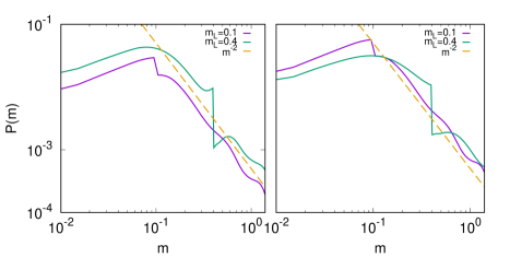
Figure 1: Overall wealth distribution $P(m)$ for model A (Left) and model B (right) for $m_{L}=0.1$ (violet), $0.4$ (green). The Pareto exponent $\nu$ is found to be close to $1$.

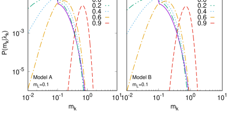
Figure 2: Left: Wealth distribution for model A for $m_{L}=0.1$ for $\lambda_{k}=0.0$(violet),$0.2$(green),$0.4$(blue),$0.6$(yellow), $0.9$(red), Right: Wealth distribution for model B for same $m_{L}=0.1$ and same $\lambda_{k}$ s. Both are for a tagged BTL agent. The plots indicate higher probability close to $m_{L}$.

III Agent Dynamics

Although the actual form of wealth distribution $P(m)$ depends on the form of saving propensity distribution, there is one thing common for all. The Pareto tail is present whatever be the form of the saving propensity distribution; the only difference is in the value of the exponent. Here, the saving propensities of all the agents are chosen from a uniform distribution which is the simplest one. Although in this work, we are actually interested in the dynamics of a tagged agent, the behaviour of overall distribution of wealth $P(m)$ is also of great importance. The overall wealth distribution shows the Pareto exponent to be roughly $1$ as in case of conventional CCM model [13] except from the fact that near $m_{L}$ there is a sharp change in the profile. This behaviour can be understood by studying individual agent’s wealth distribution which will be addressed in the next section. The wealth distribution $P(m)$ is shown in Fig. 1 for model A (Left) and model B (right) for two different $m_{L}$.

We perform numerical simulation for a system of $N$ agents and look for the dynamics of a tagged agent who is a BTL one with a predefined saving propensity. As we have stated earlier we use two models, namely A and B, for assigning subsidy.

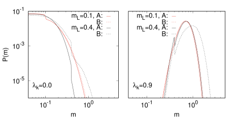
Figure 3: Left: Wealth Distribution of the BTL tagged agent for both models A and B for $\lambda_{k}=0.0$. Right: Same for $\lambda_{k}=0.9$. The data are shown for $m_{L}=0.1$(red), $0.4$ (black). The plots indicate that for model B the wealth distribution extends upto a larger $m$ as we are repeating the wealth assignment. The effect is more prominent for larger values of $m_{L}$.

III.1 Wealth Distribution

The distribution of wealth $P(m_{k}|\lambda_{k})$ for different $\lambda_{k}$ of the tagged BTL agent are shown in Fig. 2 for both the models A and B for $m_{L}=0.1$. For both the cases the nature of wealth distribution is similar to what observed in [35] and earlier [13, 26] with the exception that as the tagged agent is a BTL one and she/he is assigned a wealth equal to $m_{L}$, there is a higher probability near $m_{L}$ than what observed earlier. For small values of $\lambda_{k}$ the agent has a small amount of wealth compared to the average wealth of the economy and for higher $\lambda_{k}$ the wealth possessed by the agent is comparable to the average wealth. It is to be noted that as our agent is a BTL one, the average wealth she/he possessed is smaller compared to that predicted by the usual CCM model. As we increase $m_{L}$ to higher values, higher $m$ is more probable. The models A and B show similar distribution for all $\lambda_{k}$ if $m_{L}$ is low but their nature is different for higher $m_{L}$. It is seen that for higher threshold line the distribution for model B shifts to higher $m$ compared to model A. This can be understood easily. For model B, we are assigning the subsidy to BTL agents at every MC steps without checking whether they are below the threshold line or not. Therefore, higher value of wealth is more probable. This can also be realized from another aspect of the CCM model. When we set a higher $m_{L}$, that means a larger number of agents is below that line compared to the case of a smaller $m_{L}$. That means we are moving closer to the usual CCM picture where we choose an agent irrespective of the initial wealth possessed by her/him. These are shown in Fig. 3 for $m_{L}=0.1$ and $m_{L}=0.4$ for $\lambda_{k}=0.0,0.9$.

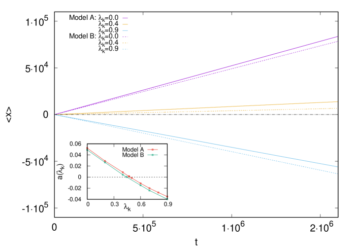
Figure 4: Variation of $\langle x\rangle$ against $t$ for $\lambda_{k}=0.0$ (violet),$0.4$ (yellow) and $0.9$ (blue) for the BTL tagged agent walker for both models A (solid lines) and B (dotted lines) for $N=256$ for $m_{L}=0.1$. Inset shows the plot of slope $a(\lambda_{k})$ as a function of $\lambda_{k}$ obtained from the slopes of $\langle x\rangle$ versus $t$ plot for the walker for both the models A and B.

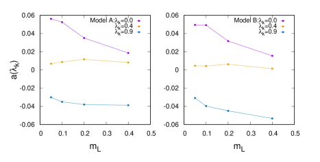
Figure 5: Variation of $a(\lambda_{k})$ against $m_{L}$ for $\lambda_{k}=0.0$ (violet),$0.4$ (yellow) and $0.9$ (blue) for the BTL tagged agent walker for both models A (Left) and B (Right) for $N=256$.

IV Walk in the GLS: Comparison to a Lazy Walker

To investigate the dynamics of this model in more detail at the microscopic level, one may conceive a walk for the agents in the GLS. It is well known that the usual CCM walk can be compared to a biased random walk (BRW) whose forward bias decreases as we increase $\lambda$ from zero. The walk has no bias at a particular $\lambda_{k}=0.469$ and then it decreases further and becomes negative on increasing $\lambda_{k}$ [35, 36]. The steps in those studies were taken as Right/Left according to whether it is Gain/Loss. In this study we are going to take a similar approach for this CCM walk with a modification. Except for Gain and Loss, there is a third possibility. When an agent gains she/he moves a step towards Right and if she/he incurs a loss moves a step towards Left. Apart from these two, the third possibility demands that the BTL tagged agent may not interact with another one if any one of them or both possesses a wealth less than $m_{L}$ and therefore the corresponding walker may stay put at its position in the GLS. The walks are correlated as when two agents interact, if any one takes a right step, the other has to move towards left. Also if one is stay put, the other should stay put too.

IV.1 Measurement of bias

For a lazy walker we know that it can have steps $1,0,-1$. It is obvious therefore that the CCM walk in this study can be compared to a lazy walk. If the agent gains then the corresponding walker moves one step to the right, if loses, the walker moves towards left. If the interaction is missed due to either one of them or both falling below the threshold line, the walker remains in its position in the GLS. Just like earlier works, here also the amount of gain/loss is not important.

Consider a biased lazy walker with probability of going towards right $p_{R}$, towards left $p_{L}$ and probability to stay put $p_{0}$. Obviously $p_{R}+p_{L}+p_{0}=1$. The average distance traveled by such a walker is linear in $t$. Precisely, the average distance traversed can be written as $\langle x\rangle=a(\lambda_{k})t$. Here $a(\lambda_{k})=[2p_{R}-(1-p_{0})]$ is the slope of the line, a measure for the amount of drift. As in any ballistic diffusion, here we have $(\langle x^{2}\rangle-\langle x\rangle^{2})\sim t^{2}$ for all $\lambda_{k}$ except when $\lambda_{k}\rightarrow\lambda_{k}^{*}$. For $\lambda_{k}\rightarrow\lambda_{k}^{*}$, we have observed that $(\langle x^{2}\rangle-\langle x\rangle^{2})\sim t$. In Fig. 4, the variation of $\langle x\rangle$ against $t$ is shown for $\lambda_{k}=0.0,0.4$ and $0.9$ for the BTL tagged agent walker for both models A and B. Here we have taken $N=256$ and $m_{L}=0.1$. Inset shows the plot of drift $a(\lambda_{k})$ as a function of $\lambda_{k}$. The drifts are obtained from the slopes of $\langle x\rangle$ versus $t$ plot. At $\lambda_{k}^{*}$, for both the models we have found that $p_{R}=p_{L}$ and therefore drift $a(\lambda_{k}^{*})=0$. The precise value of $\lambda_{k}^{*}$ is found to be $0.471$ for model A and $0.443$ for model B. For any $\lambda_{k}$ the slope is more positive for low $m_{L}$ and less positive for larger $m_{L}$. However, close to $\lambda_{k}^{*}$, the effect is almost negligible. This is shown in Fig. 5. This can be interpreted in the following way. The BTL agents’ subsidy come from other agents’ taxes, i.e., at the cost of others. As we increase $m_{L}$, number of BTL agents increase and the subsidy amount coming from the taxes of others increase. Therefore possibility of having an interaction decreases and the tendency to gain also decreases. As our definition for model B demands giving subsidy to the agent at every MC step, and that has to come from the others above the threshold line, therefore, the effect is more pronounced for model B compared to A. However, the amount of wealth possessed by a BTL agent increases as we increase $m_{L}$ for any specific $\lambda_{k}$.

We check the exact number of right, left and zero steps for the modified CCM walk and try to find out how the probabilities $p_{R},p_{L},p_{0}$ change with $\lambda_{k}$ for a specific $m_{L}$. As we know that $a(\lambda_{k})=2p_{R}-(1-p_{0})$, from Fig. 4 it is clear that, $p_{R},p_{L}$ and $p_{0}$ are functions of $\lambda_{k}$. The specific probabilities for two $m_{L}$ values will be found in the Table 1. For both the models the variation of $p_{0}(\lambda_{k})$ against $\lambda_{k}$ are shown in Fig. 6 for two different $m_{L}$. It is seen that the nature of variation matches well with the form $p_{0}(\lambda_{k})\sim a_{0}\exp(-b_{0}x^{2})$ for both the models A and B, where $a_{0}$ and $b_{0}$ are two parameters, for low values of $\lambda_{k}$. The plots show discrepancy for high $\lambda_{k}$ values from the predicted behaviour. Now if we simulate a lazy walker with those $p_{0},p_{R}$ and $p_{L}$ values that should show a similar $\langle x\rangle$ versus $t$ behaviour. In the inset of Fig. 6, the $\langle x\rangle$ versus $t$ graph is compared with the same of a lazy walker for a few specific $\lambda_{k}$ and therefore $p_{0},p_{R}$ and $p_{L}$ values values.

Table 1: $p_{0},p_{R},p_{L}$ values for specified $m_{L}$ and $\lambda_{k}$ values for Model A and B for the modified CCM walker of BTL agent.

$m_{L}$	$\lambda_{k}$	Model A			Model B
		$p_{0}$	$p_{R}$	$p_{L}$	$p_{0}$	$p_{R}$	$p_{L}$
0.1	0.0	0.285	0.384	0.331	0.282	0.386	0.332
	0.4	0.111	0.449	0.439	0.113	0.446	0.441
	0.9	0.0	0.482	0.518	0.0	0.480	0.520
0.05	0.0	0.078	0.492	0.430	0.110	0.474	0.416
	0.4	0.013	0.496	0.490	0.020	0.492	0.488
	0.9	0.0	0.481	0.519	0.0	0.480	0.520

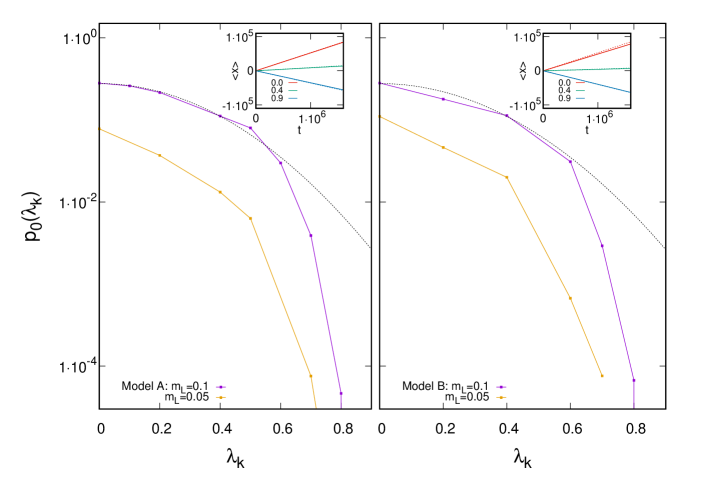
Figure 6: Variation of $p_{0}(\lambda_{k})$ against $\lambda_{k}$ for models A (Left) and B (Right) for $N=256$ for $m_{L}=0.05$ (yellow), $0.1$ (violet). Black dotted line shows the nature of $a_{0}\exp(-b_{0}x^{2})$. Inset shows the comparison of slope obtained from $\langle x\rangle$ versus $t$ data (solid line) and using the parameters in lazy walk (dotted line).

IV.2 Distribution of Path Lengths in the GLS

We have seen in the previous section, how the probabilities $p_{R},p_{L},p_{0}$ changes with $\lambda_{k}$. To have a detailed understanding about the probabilities we are now going to study how the quantities vary with walk length $X$. A path length $X$ here signifies the length traversed at a stretch without changing direction. For the Right/Left direction, this means the agent will gain/lose for $X$ steps continuously and after that it will either make a loss/gain or stay put. Here we study three such quantities $W_{R}(X),W_{L}(X)$ and $W_{0}(X)$ where the suffix indicates whether it is a gain or loss or no interaction. The distribution of path lengths in the GLS is an interesting quantity to study and was studied earlier in [36] where there were only Right/Left movements. Here, it is clear that:

$$W_{i}(X)\propto p_{i}^{X}(1-p_{i})^{2};~{}~{}~{}~{}~{}~{}i=0,R,L.\\$$ (3)

We now wish to extract the values of $p_{R}$ for a specific $\lambda_{k}$ and $m_{L}$ from the distribution of path lengths at a stretch. For high $\lambda_{k}$ values, e.g., $\lambda_{k}=0.8,0.9$, the probability $p_{0}$ is extremely small, and therefore the walk is very similar to a biased random walk. In that case, it is easy to extract some $p_{R}^{eff}(X,\lambda_{k},m_{L})$ as then we can approximately write

$$\frac{W_{R}(X)}{W_{L}(X)}=(\frac{p_{R}}{1-p_{R}})^{X-2}.$$ (4)

$\frac{W_{R}(X)}{W_{L}(X)}$ is calculated numerically for a $\lambda_{k}$ and $m_{L}$. The $p_{R}^{eff}$ is shown as a function of $X$ in Fig. 7 for a few $m_{L}$ values for both model A and B. The $p_{R}$ value has some variation over $X$ and not constant as predicted in Table 1.

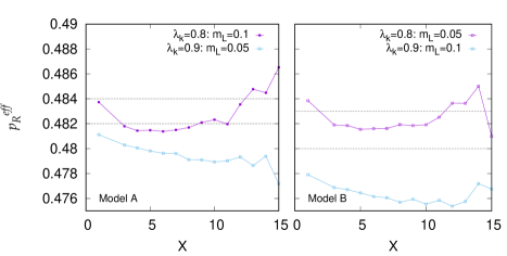
Figure 7: Variation of $p_{R}^{eff}$ as a function of $X$ for models A ($\lambda_{k}=0.8,m_{L}=0.1$ (violet) and $\lambda_{k}=0.9,m_{L}=0.05$ (blue) shown) and B ($\lambda_{k}=0.8,m_{L}=0.05$ and $\lambda_{k}=0.9,m_{L}=0.1$ shown) for $N=256$ obtained by distribution of walk lengths at a stretch. Black dotted lines show the corresponding $p_{R}$ values obtained from slopes.

For smaller $\lambda_{k}$ however we cannot use Eq. 4. As for a lazy walker there are three parameters involved, we can use the obtained value of $p_{0}$ to check whether we are getting the same $p_{R}$ value as in Table 1 from this path length distribution data or not. For this we use the following:

$$\frac{W_{R}(X)}{W_{0}(X)}=\frac{p_{R}^{X}(1-p_{R})^{2}}{p_{0}^{X}(1-p_{0})^{2}}.$$ (5)

For the BTL tagged agent’s walk in GLS, we calculate $\frac{W_{R}(X)}{W_{0}(X)}$ numerically for specific values of $\lambda_{k}$ and $m_{L}$. The obtained $p_{R}^{eff}(X,\lambda_{k},m_{L})$ values do not match well except for the low values of $X$.

From the above two aspects, therefore, we can say that the walker is not behaving like an usual biased lazy walker. The variation of $W_{0},W_{R}$ and $W_{L}$ as a function of $X$ are shown in Fig. 8 a, b for A and B. As it can be seen the individual path distributions vary approximately as an exponential. It is to be noted here that all the variations are shown such that $\sum_{X}W_{i}(X)=1$ where $i=0,R,L$. Also the relative variation of path distributions $W_{0},W_{R}$ and $W_{L}$ as a function of $X$ are shown in Fig. 8 c, d, considering $W_{0}(X)+W_{R}(X)+W_{L}(X)=1$ for all $X$. It is clear from Fig. 8 c, d that for large $X$, $W_{R}$ and $W_{L}$ decreases and finally comes to zero. That means long paths at a stretch for Gain/Loss are less probable. However, long $W_{0}$ paths are possible.

Figure 8: Top Left : Variation of $W_{0}(X)$ against $X$ for models A and B for $\lambda_{k}=0.0,0.4$ and $m_{L}=0.1$ (violet and blue for model A and green and yellow for model B). Top Right : Variation of $W_{R}(X)$ (violet and blue) and $W_{L}(X)$ (green and yellow) against $X$ for model A for $\lambda_{k}=0.0,0.4$ and $m_{L}=0.1$. (Behaviour of the quantities for model B is similar as those of A and therefore it is not shown.) Bottom Left : Relative variation of $W_{0}(X)$ (violet), $W_{R}(X)$ (red), $W_{L}(X)$ (green) against $X$ for model A for $\lambda_{k}=0.0,0.4$ and $m_{L}=0.1$. Bottom Right : Relative variation of $W_{0}(X)$ (violet), $W_{R}(X)$ (red), $W_{L}(X)$ (green) against $X$ for model B for $\lambda_{k}=0.0,0.4$ and $m_{L}=0.1$.

Figure 9: Left : Direction Reversal Probability $f_{d}$ against $\lambda_{k}$ for model A for $m_{L}=0.1$ (violet) , $m_{L}=0.05$ (yellow). Solid lines indicate $f_{d}$ from distribution of free path and dashed lines indicate those from the simulated lazywalk. Right : Same for Model B

Another interesting quantity to check here is the direction reversal probability. For lazy walker, the direction reversal probability is $2(p_{0}+p_{R}-p_{0}^{2}-p_{R}^{2}-p_{0}p_{R})$. For our walk we consider the following quantity:

$$\langle X\rangle=\sum_{X}(XW_{R}(X)+XW_{L}(X)+XW_{0}(X)).$$ (6)

Here $\langle X\rangle$ is the average distance traveled in any particular direction (Gain, Loss or no movement) at a stretch. Obviously, the direction reversal probability is given by $f_{d}=\frac{1}{\langle X\rangle}$.

The results are shown for some specific $\lambda_{k}$ and $m_{L}$ for A and B. It is seen that for our walker, probability is very high for all $\lambda_{k}$ values which saturates to a value close to $0.5$ for high $\lambda_{k}$. This is expected as when $\lambda_{k}$ is high, number of missed interactions become negligible. Therefore, the dynamics is controlled only through $p_{R}$ and the situation becomes similar as in case of Right/Left movement. These are shown in Fig. 9. We also simulated a lazy walk using the parameters $p_{0},p_{R},p_{L}$ and calculated $f_{d}$ for that. For the lazy walker although the nature of variation is similar and tends to $0.5$ for high $\lambda_{k}$ as in case of our walker, the exact probabilities do not match.

V Correlation

We have seen that the steps of the walker have three possible values. Therefore, we need to analyze the time series for such a walk. Let the step taken at a time $t$ be written as $s(t)=0,\pm 1$. The corresponding time correlation function can be written as: $C(t)=\langle s(t_{0})s(t_{0}+t)\rangle-s_{0}^{2}$ where $s_{0}^{2}=\langle s(t_{0})\rangle\langle s(t_{0}+t)\rangle$. This can be written as we know that here $\langle s(t_{0})\rangle$ is independent of $t$ and therefore $\langle s(t_{0})\rangle=\langle s(t_{0}+t)\rangle=s_{0}$. Just as in CCM walk, here $\langle s_{0}\rangle\neq 0$ unless near $\lambda_{k}^{*}$ for both the model A and B. The correlations for model A and B are shown in Fig. 10. It is seen that there is a strong correlation near $t=1$ which gradually decreases with increasing $\lambda_{k}$.The short time correlations in both models A and B are negative. This is consistent with the fact that direction reversal probability is greater than $1/2$. However, for one particular $\lambda_{k}$ the correlation ultimately saturates to a value $C_{sat}$ when $t\rightarrow\infty$.

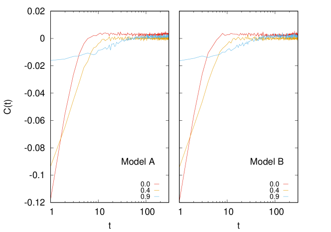
Figure 10: Left : The correlation of steps $C(t)$ averaging over all possible initial times $t_{0}$ for the walker for model A for $m_{L}=0.1$ and $\lambda_{k}=0.0$ (red), $0.4$ (yellow), $0.9$ (blue). Right : Same for Model B.

Figure 11: Left : The saturation value of correlation of steps $C_{sat}$ against $\lambda_{k}$ for $m_{L}=0.1$ for A (violet) and B (yellow). Middle : The strongest correlation $C(1)$ as a function of $\lambda_{k}$ for $m_{L}=0.1$ for the models A (red) and B (black). Right : $C(1)$ against $m_{L}$ for A (green) and B (yellow) for $\lambda_{k}=0.0$ (solid line) and $\lambda_{k}=0.4$ (dashed line).

This kind of feature was earlier noticed in [36]. The saturation value $C_{sat}$ is estimated by averaging near the end over a few hundred values of $t$. $C_{sat}$ as a function of $\lambda_{k}$ is shown for $m_{L}=0.1$ for both models A and B in Fig. 11 a. It is seen that $C_{sat}$ reaches a minimum close to $\lambda_{k}^{*}$ which is $0.471$ for model A and $0.443$ for model B. The minimum value of $C_{sat}$ as observed for a $\lambda_{k}\approx\lambda_{k}^{*}$ is $\sim O(10^{-5})$. Also as we observe the strongest correlation $C(1)$ is changing with $\lambda_{k}$, we plot the same in Fig. 11 b. It is observed that as we increase threshold line $m_{L}$, the correlation over one step $C(1)$ becomes weaker and weaker for lower $\lambda_{k}$ values. However for high $\lambda_{k}$ for all $m_{L}$ values, $C(1)$ is almost a constant. This feature is similar in model A and B but for higher values of $m_{L}$ the strength of maximum correlation, i.e., $C(1)$ is weaker for a particular $m_{L}$ in model $B$. This is shown in Fig. 11 c.

VI Reason Behind High Direction Reversal

It is already seen that the probability of direction reversal in the GLS is very high. This signature is also clear from the strong correlation for small $t$. In this part, we are going to analyze why this direction reversal is preferred by an agent in this walk.

For our convenience, we choose the DY model which is the simplest among all and the form of wealth distribution is well known. For this we mimic a situation when the agent ends up with gain and then again interacts. The probability that the agent will incur a loss in the next step requires that she/he has to interact with another with low value of wealth. We consider our agent ends up with wealth $m^{\prime}$ in the first step. However, there are two possibilities in this case. If the second agent’s wealth is between $0$ and $m_{L}$ then there will be no interaction at all and if that is higher than $m_{L}$ and less than $m^{\prime}$, our agent may lose some. The conditional probability that the agent will have a loss after a gain is

$$W^{\prime}(LG)=\frac{\int_{m_{1}}^{\infty}P(m_{1})dm_{1}\int_{m_{L}}^{m_{1}}P(m_{2})dm_{2}}{\int_{m_{1}}^{\infty}P(m_{1})dm_{1}}$$ (7)

and the probability that the interaction will not occur is

$$W^{\prime}(0G)=\frac{\int_{m_{1}}^{\infty}P(m_{1})dm_{1}\int_{0}^{m_{L}}P(m_{2})dm_{2}}{\int_{m_{1}}^{\infty}P(m_{1})dm_{1}}$$ (8)

But the probability that the previous step was a gain is $p_{R}$. Considering the wealth distribution of the form $P(m)\sim\exp(-m)$, the probability that it will either lose or stay put is $W(iG)=p_{R}(\lambda_{k})\times(1-\frac{1}{2}\exp(-m_{1}))$ where $i=L/0$.

Similarly the conditional probability of having a Loss in the first step and then either a Gain or a no interaction is

$$W^{\prime}(jL)=\frac{1}{2}[1+\exp(-m_{1})]+1-\exp(-m_{L})$$ (9)

where $j=G/0$. Therefore $W(jL)=p_{L}(\lambda_{k})W^{\prime}(jL)=p_{L}(\lambda_{k})[\frac{1}{2}[1+\exp(-m_{1})]+1-\exp(-m_{L})]$.

Proceeding in a similar manner we can show that

$$W(i0)=p_{0}(\lambda_{k})$$ (10)

where $i=G/L$.

Thus, the probability of direction reversal is

$$f_{d}(\lambda_{k})=p_{0}(\lambda_{k})+p_{R}(\lambda_{k})(1-\frac{1}{2}\exp(-m_{1}))+p_{L}(\lambda_{k})[\frac{1}{2}[1+\exp(-m_{1})]+1-\exp(-m_{L})].$$ (11)

In any case we can show that

$$f_{d}(\lambda_{k})>p_{0}(\lambda_{k})+\frac{1}{2}p_{R}(\lambda_{k})+p_{L}(\lambda_{k})[\frac{3}{2}-\exp(-m_{L})]$$ (12)

Using the obtained values of $p_{0},p_{R}$ and $p_{L}$ for different $\lambda_{k}$ and $m_{L}$ we check the lower bound of the direction reversal probabilities from the Eq. 12. $f_{d}$ for a few $\lambda_{k}$ and $m_{L}$ values obtained using Eq. 12 and from the model are compared in Table 2.

Table 2: Comparison of direction reversal probabilities $f_{d}$ obtained from Eq. 12 and from the model A

$m_{L}$	$\lambda_{k}$	$f_{d}$
		From Eq. 12	From Lazywalk	From model
0.1	0.0	0.672	0.661	0.580
	0.4	0.598	0.593	0.593
	0.9	0.548	0.499	0.508
0.05	0.0	0.560	0.567	0.600
	0.4	0.530	0.513	0.552
	0.9	0.525	0.499	0.508

As we can see from Table 2, there is good agreement of the lower bound of the inequality with the lazy walker except when $\lambda_{k}$ is very high. Also the agreement is not that good for the data obtained from our model. This indicates that the walk of our agent is not exactly a lazy walk. As $\lambda_{k}$ becomes very high the DY model approximation is no longer valid and therefore there is discrepancy from the direction reversal probability obtained from Eq. 12.

VII Summary and Conclusion

In this work, the nature of transactions made in CCM model with some modification is studied. We used the idea of threshold line below which an agent is identified as a BTL one at the time of assigning wealth. These agents are always eligible for subsidy. This is similar to giving opportunity to some backward class people in any caste-based system. The threshold line is important in another way. It dictates whether an interaction will occur or not. Any agent, either BTL or not, having wealth below that line at any point of interaction is considered insecure as in any real situation. If either one or both the interacting agents’ wealth is below the threshold line, the interaction will not occur. We also considered an equivalent picture of a $1$D walk in an abstract space for Gains and Losses. Here amount of Gain/Loss is not important; we have just used the information whether it is a Gain or Loss. As a tagged agent may have Gain, Loss or no interaction, the corresponding walker is a lazy walker which in addition to Left/Right movement, may stay put at a position. The high direction reversal probability indicates that there is a high tendency of individuals to make a gain or to stay put immediately after a loss and vice versa. This kind of effect was studied for usual CCM model before. Here also we found this to be compatible with human psychology. From the high direction reversal probability it is clear that after a ’no’ interaction the agent will try to interact immediately at the next step. Also a person may take part in an interaction which may lead either to a loss or to no interaction, when she/he had a gain in the previous step. After suffering a loss, in a same manner, a person will either try to have a gain or may stay put due to insecurity. This effect is maximum for zero saving propensity and decreases with increased saving. The data obtained from correlation for one step also indicates that there will be high tendency of gain after loss and vice versa. (of course, there may be stay puts in between).

The subsidy is given here in two ways, firstly at the time of assigning the wealth to the agents initially (Model A), and secondly, at each MC step (Model B). It is seen that if subsidy is given repeatedly (i.e., at each MC step), the agent moves with a less positive drift in the GLS for Model B compared to Model A for any particular $\lambda_{k}$ (Fig. 4). This can be understood, as, giving repeated subsidy to a BTL agent will affect the wealth of others and as the walks are actually correlated, it affects the tagged BTL walk in turn. The amount of wealth possessed by such an agent is greater in Model B compared to Model A. The parameters $p_{0},p_{R}$ and $p_{L}$ are obtained from the walk of the tagged BTL agent and with those a lazy walk is simulated. It is seen that the BTL agent’s CCM-like walk is not exactly similar to a biased lazy walk. The walk has no bias for some saving propensity $\lambda_{k}^{*}$ which is different for models A and B.

The distribution of path traveled at a stretch $X$ is studied for Right/Left movements and staying put. The quantities are $W_{R}(X),W_{L}(X)$ and $W_{0}(X)$ where the suffix indicates whether it is a gain or loss or no interaction. Using that we calculated the direction reversal probability $f_{d}$ and the same is calculated analytically for a DY model. Using the lazy walker parameters we compared the analytical direction reversal probability with those obtained from the walk. The analytical approach indicates that $f_{d}(\lambda_{k})$ must be greater than $p_{0}(\lambda_{k})+\frac{1}{2}p_{R}(\lambda_{k})+p_{L}(\lambda_{k})[\frac{3}{2}-\exp(-m_{L})]$. However, the analytical treatment was done using the DY model wealth distribution and therefore is not in good agreement to our case, when saving propensity is high. From different calculations shown here it is clear that for Model A, $\lambda_{k}=\lambda_{k}^{*}\simeq 0.471$ and for model B it is close to $0.443$. Although for Model A it is close to the $\lambda_{k}^{*}$ obtained for usual CCM model, i.e., $0.469$, for Model B the result is different.

Finally, our study shows a modified CCM model with the concept of a Threshold line. The threshold line in addition to identification of BTL agents, puts restriction to interactions. We have seen that putting restriction changes the distribution which is dependent on the threshold line $m_{L}$ as shown in Fig. 3. The dynamics of a tagged BTL agent is compared to a Lazy walker in GLS. The high direction reversal probability for such a walker indicates that one can afford to have a loss or may stay put he/she has gained begore. Also after suffering a loss, it may stay put or may try to make a gain. This is completely compatible with human psychology. Also, it is seen that the value of $\lambda_{k}^{*}$ is independent of $m_{L}$ for both the models A and B as shown in Fig. 5. The effect of giving subsidy once over giving repeated subsidy to such agents is checked from the point of view of the walk in GLS. The walk is seen to have more positive drift when the subsidy is given once.

References

- [1] Pareto V. 1897 Cours d’economie Politique. Paris, Lausanne : Rouge F.
- [2] Madelbrot BB. 1960 The Pareto-Levy Law And The Distribution Of Income. Int. Econ. Rev. 1, 79-106.
- [3] Chakrabarti BK, Chakraborti A, Chakravarty SR, Chatterjee A. 2013 Econophysics of Income and Wealth Distributions. Cambridge, Cambridge University Press.
- [4] Chatterjee A, Yarlagadda S, Chakrabarti BK, eds. 2005 Econophysics of Wealth Distributions. Milan, Springer Verlag.
- [5] Chakrabarti BK, Chakraborti A, Chatterjee A, eds. 2006 Econophysics and Sociophysics. Berlin, Wiley-VCH.
- [6] Sinha S, Chatterjee A, Chakraborti A, Chakrabarti BK. 2010. Econophysics: An Introduction. Berlin, Wiley-VCH.
- [7] Yakovenko VM, Barkley Rosser J Jr. 2009 Colloquium: Statistical mechanics of money, wealth, and income. Rev. Mod. Phys. 81, 1703-1725.
- [8] Silva AC, Yakovenko VM. 2005 Temporal evolution of the ”thermal” and ”superthermal” income classes in the USA during 1983-2001. Europhys. Letts. 69(2), 304-310.
- [9] Drăgulescu AA, Yakovenko VM. 2001 Evidence for the exponential distribution of income in the USA. Eur. Phys. J. B 20, 585-589; Drăgulescu AA, Yakovenko VM. 2001 Exponential and power-law probabilitydistributions of wealth and income in the UnitedKingdom and the United States. Physica A 299, 213-221); Levy M, Solomon S. 1997 New evidence for the power-law distribution of wealth. Physica A 242(1), 90-94; Sinha S. 2006 Evidence for Power-law tail of the Wealth Distribution in India. Physica A 359, 555-562; Aoyama H, Souma W, Fujiwara Y. 2003 Growth and fluctuations of personal and company’s income Physica A 324 (1-2), 352-358; Matteo TD, Aste T, Hyde ST. 2004 Exchanges in complex networks: income and wealth distributions IN The Physics of Complex Systems (New Advances and Perspectives), (eds Mallamace F, Stanley HE), pp. 435-442. Amsterdam, IOS Press; Clementi F, Gallegati M. 2005 Power Law Tails in the Italian Personal Income Distribution. Physica A 350 (2-4), 427-438; Ding N, Wang Y. 2007 Power-Law Tail in the Chinese Wealth Distribution. Chinese Phys. Letts. 24, 2434-2436.
- [10] Chakrabarti BK, Marjit S. 1995 Self-organisation in Game of Life and economics. Ind. J. Phys. B 69, 681-698; Ispolatov S, Krapivsky PL, Redner S. 1998 Wealth Distributions in Asset Exchange Models. Eur. Phys. J. B 2, 267-276.
- [11] Drăgulescu AA, Yakovenko VM. 2000 Statistical mechanics of money. Eur. Phys. J. B 17, 723-729.
- [12] Chakraborti A, Chakrabarti BK. 2000 Statistical mechanics of money: how saving propensity affects its distribution. Eur. Phys. J. B 17, 167-170.
- [13] Chatterjee A, Chakrabarti BK, 2007 Kinetic exchange models for income and wealth distributions. Eur. Phys. J. B 60, 135-149; Chatterjee A, Sinha S, Chakrabarti BK. 2007 Economic inequality: Is it natural?. Current Science 92(10), 1383-1389.
- [14] Chatterjee A. 2010 On kinetic asset exchange models and beyond:microeconomic formulation, trade network, and all that IN Mathematical Modeling of Collective Behavior in Socio-Economic and Life Sciences(eds Naldi G. et. al.) pp. 31-50. Boston, Birkhaüser.
- [15] Torregrossa M., Toscani G. 2018 Wealth distribution in presence of debts: A Fokker-Planck description. CMS 16(2), 537-560.
- [16] Bouchaud J. P., Mézard M. 2000 Wealth condensation in a simple model of economy. Physica A 282(3-4), 536-545.
- [17] Solomon S, Richmond P. 2001 A simple model of bank bankruptcies. Physica A 299 (1-2), 188-197.
- [18] Malcai O, Biham O, Richmond P, Solomon S. 2002 Theoretical analysis and simulations of the generalized Lotka-Volterra model. Phys. Rev. E 66, 031102.
- [19] Garlaschelli D, Loffredo MI. 2008 Effects of network topology on wealth distributions. J. Phys. A : Math Theor. 41, 224018.
- [20] Sornette D, Cont R. 1997 Convergent Multiplicative Processes repelled fom zero : power laws and truncated power laws. J. Phys. I 7, 431-444.
- [21] Toscani G., Tosin A., Zanella M. 2020 Kinetic modelling of multiple interactions in socio-economic systems. Netw. Heterog. Media, 15(3), 519-542.
- [22] Bachelier L. 1900 Théorie de la spéculation. Ann. Sci. Ecole Norm. Sup. 3, 21-86.
- [23] Saha MN, Srivastava BN. 1931 A Treatise on Heat. Allahabad, Indian Press.
- [24] Patriarca M, Chakraborti A, Kaski K. 2004 Statistical model with a standard distribution. Phys. Rev. E 70, 016104.
- [25] Repetowicz P, Hutzler S, Richmond P. 2005 Dynamics of money and income distributions. Physica A 356, 641-654.
- [26] Chatterjee A, Chakrabarti BK, Manna SS. 2004 Pareto Law in a Kinetic Model of Market with Random Saving Propensity. Physica A 335, 155-163; 2003 Money in Gas-Like Markets: Gibbs and Pareto Laws. Phys. Scr. T 106, 36-38.
- [27] Tumminello M, Lillo F, Piilo J, Mantegna RN. 2012 Identification of clusters of investors from their real trading activity in a financial market. New Journal of Physics 14 013041.
- [28] Gabaix X, Gopikrishnan P, Plerou V, Stanley HE. 2003 A Theory of Large Fluctuations in Stock Market Activity. MIT Working Paper Series 3-30, 1-46.
- [29] Chakraborty A, Manna SS. 2010 Weighted trade network in a model of preferential bipartite transactions. Phys. Rev. E 81, 016111.
- [30] Goswami S, Sen P. 2014 Agent based models for wealth distribution with preference in interaction. Physica A 415, 514-524.
- [31] Dimarco G., Pareschi L., Toscani G., Zanella M. 2020 Wealth distribution under the spread of infectious diseases. Phys. Rev. E 102, 02230.
- [32] Ferrero J. C. 2010 The individual income distribution in Argentina in the period 2000-2009. A unique source of non stationary data. arXiv:1006.2057.
- [33] Govt. of India Planning Commission. 2014 Report of The Expert Group to Review The Methodology for Measurement of Poverty.
- [34] Brady D, Fullerton AS, Cross JM. 2009 Putting Poverty in Political Context: A Multi-Level Analysis of Adult Poverty across 18 Affluent Democracies. Social Forces 88(1), 271-299.
- [35] Chatterjee A, Sen P. 2010 Agent dynamics in kinetic models of wealth exchange. Phys. Rev. E 82, 056117.
- [36] Goswami S, Chatterjee A, Sen P. 2011 Antipersistent dynamics in kinetic models of wealth exchange. Phys. Rev. E 84, 051118.