A global QCD analysis of diffractive parton distribution function considering higher twist corrections within the xFitter framework

Abstract

We present SKMHS22, a new set of diffractive parton distribution functions (PDFs) and their uncertainties at next-to-leading-order accuracy in perturbative QCD within the xFitter framework. We describe all available diffractive DIS data sets from HERA and the most recent high-precision H1/ZEUS combined measurements considering three different scenarios. First, we extract the diffractive PDFs considering the standard twist-2 contribution. Then, we include the twist-4 correction from the longitudinal virtual photons. Finally, the contribution of subleading Reggeon exchange to the structure-function $F_{2}^{D}$ is also examined. For the contribution of heavy flavors, we utilize the Thorne-Roberts general mass variable number scheme. We show that for those corrections, in particular, the twist-4 contribution allows to include the high-$\beta$ region and leads to a better description of the diffractive DIS data sets. We find that the inclusion of the subleading Reggeon exchange significantly improves the description of the diffractive DIS cross-section measurements. The resulting sets are in good agreement with all diffractive DIS data analyzed, which cover a wider kinematical range than in previous fits. The SKMHS22 diffractive PDFs sets presented in this work are available via the LHAPDF interface. We also make suggestions for future research in this area.

I Introduction

One of the most important experimental findimgs reported by the H1 and ZEUS collaborations at the HERA collider, working at the center of the mass-energy of about $\sqrt{s}=318$ GeV, is the observation of a significant fraction of about 8-10% of large rapidity gap events in a diffractive deep inelastic scattering (DIS) processes ZEUS:2008xhs ; H1:2006zyl ; ZEUS:2009uxs ; H1:2006zxb ; H1:2007oqt .

Such diffractive DIS processes allow us to define a non-perturbative diffractive parton distribution functions (diffractive PDFs) that can be extracted from a QCD analysis of relevant data H1:2006zyl ; ZEUS:2009uxs . According to the factorization theorem, the diffractive cross-section can be expressed as a convolution of the diffractive PDFs and partonic hard scattering cross-sections of the subprocess which is calculable within perturbative QCD.

The diffractive PDFs have properties very similar to the standard PDFs, especially they obey the same standard DGLAP evolution equation Dokshitzer:1977sg ; Gribov:1972ri ; Lipatov:1974qm ; Altarelli:1977zs . However, they have an additional constraint due to the presence of a leading proton (LP) in the final state of diffractive processes, $\ell(k)+p(P)\rightarrow\ell(k^{\prime})+p(P^{\prime})+X(p_{X})$.

Considering the diffractive factorization theorem, the diffractive PDFs can be extracted from the reduced cross-sections of inclusive diffractive DIS data by a QCD fit. It should be noted here that if the factorization theorem would be violated in hadron-hadron scattering, then there is no universality for example for the diffractive jet production in hadron-hadron collisions Collins:1992cv ; Wusthoff:1999cr . Starting from perturbative QCD, in the first approximation, diffractive DIS is described in the dipole framework and formed by the quark-antiquark (${q}\bar{{q}}$) and quark-antiquark-gluon (${q}\bar{q}$) system.

So far all, several groups extracted the diffractive PDFs from QCD analyses of the diffractive DIS data at the next-to-leading order (NLO) and next-to-next-to-leading order (NNLO) accuracy in perturbative QCD Goharipour:2018yov ; Khanpour:2019pzq ; ZEUS:2009uxs ; Ceccopieri:2016rga ; H1:2006zyl ; Maktoubian:2019ppi . In Ref. Goharipour:2018yov , the authors presented the first NLO determination of the diffractive PDFs and their uncertainties within the xFitter framework Alekhin:2014irh ; xFitterDevelopersTeam:2022koz . Ref. Khanpour:2019pzq presented the first NNLO determination of the diffractive PDFs, and the framework of fracture functions is used in the QCD analysis Trentadue:1993ka ; deFlorian:1998rj ; Ceccopieri:2016rga . Some of these studies, such as ZEUS-2010-dPDFs ZEUS:2009uxs , also include the dijet cross-section measurement to determine the well-constrained gluon PDFs.

In this paper, we report a new QCD fit of diffractive PDFs to the HERA inclusive data in diffractive DIS at the NLO in perturbative QCD within the xFitter framework Alekhin:2014irh . The present fit also includes the high-precision H1/ZEUS combined measurements of the diffractive DIS cross-section H1:2012xlc . The inclusion of the most recent HERA combined data, together with the twist-4 corrections from the longitudinal virtual photons and the contribution of subleading Reggeon exchanges to the structure-function, provide well-established diffractive PDFs sets. We show that these corrections, in particular, the twist-4 contribution allows us to explore the high-$\beta$ region, and the inclusion of the subleading Reggeons gives the best description of the diffractive DIS data. In addition, by considering such corrections, one could relax the kinematical cuts that one needs to apply to the data.

This paper is organized in the following way: In Sec. II we discuss the theoretical framework of the SKMHS22 diffractive PDFs determination, including the computation of the diffractive DIS cross-section, the evolution of diffractive PDFs, and the corresponding factorization theorem. This section also includes our choice of physical parameters and the heavy quark contributions to the diffractive DIS processes. The higher twist contribution considered in SKMHS22 QCD analysis also discussed in detail in this section. In Sec. III we present the details of the SKMHS22 diffractive PDFs global QCD analysis and fitting methodology. Specifically, we focus on the SKMHS22 parametrization, the minimization strategy, and the method of uncertainty estimation. We also present the diffractive data set used in SKMHS22 analysis, along with the corresponding observables and kinematic cuts applied to the data samples. In Sec. IV we present in detail the SKMHS22 sets. The perturbative convergence upon inclusion of the higher twist corrections is also discussed in this section. The fit quality and the theory/data comparison are presented and discussed in this section as well. Finally, in Sec. V we summarize our findings and outline possible future developments.

II Theoretical Framework

In the following section, we describe the standard theoretical framework which is perturbative QCD (pQCD) for the typical event with a large rapidity gap (LRG) for diffractive DIS processes. We discuss in detail the calculation of diffractive DIS reduced cross-section, the relevant factorization theorem, and our approaches to consider the heavy flavors contributions. We also provide the details of the diffractive structure-function (diffractive SF) taking the twist-4 and Reggeon corrections into account.

II.1 Diffractive DIS cross section

In Fig. 1, we display the Feynman diagram for diffractive DIS in the single-photon approximation. In the neutral current (NC) diffractive DIS process $ep\rightarrow ep{X}$, we have the incoming positron or electron in the initial state in which scatters off an an incoming proton with the four-momentum ${k}$ and ${P}$, respectively. As one can see from the Feynman diagram, in the final state, the proton with the four-momentum of $P^{\prime}$ remains intact and there is a rapidity gap between the proton in the final state and the diffractive system $X$ and outgoing electron with four-momentum $k^{\prime}$.

In order to calculate the reduced diffractive cross-section for such a process, one needs to introduce the standard set of kinematical variables

$$Q^{2}=-q^{2}=({k}-{k}^{\prime})\,,\quad{y}=\frac{{P.q}}{{P.k}}\,,\quad{x}=\frac{{-q^{2}}}{{2P.q}}\,,$$ (1)

which are the photon virtuality $Q^{2}$, the inelasticity ${y}$, and the Bjorken variable $x$, respectively.

In the case of diffractive DIS, one needs to introduce an additional kinematical variable ${\beta}$ which is defined to be the momentum fraction carried by the struck parton with respect to the diffractive exchange. The kinematical variable ${\beta}$ is given by,

$${\beta}=\frac{Q^{2}}{{2}(P-P^{\prime})}=\frac{Q^{2}}{M_{X}^{2}+Q^{2}-t}\,,$$ (2)

where $M_{X}$ is the invariant mass of the diffractive final state, produced by the diffractive dissociation of the exchanged virtual photon, and the variable $t=({P}-{P}^{\prime})$ is the squared four-momentum transferred at the proton vertex.

The experimental diffractive DIS data sets are provided by the H1 and ZEUS collaborations at HERA in the form of the so-called reduced cross section $\sigma_{r}^{D3}(\beta,Q^{2};{x}_{I\!\!P},t)$, where $x_{I\!\!P}$ is defined to be the longitudinal momentum fraction lost by the incoming proton. The longitudinal momentum fraction $x_{I\!\!P}$ satisfies the relation $x={\beta}x_{I\!\!P}$. The $t$-integrated differential cross-section for the diffractive DIS processes can be written in terms of the reduced cross-section as,

$$\frac{d\sigma^{ep\rightarrow ep{X}}}{d{\beta}dQ^{2}dx_{I\!\!P}}=\frac{{2}{\pi}\alpha^{2}}{{\beta}Q^{4}}\left[1+(1-{y})^{2}\right]\sigma_{r}^{D3}({\beta},Q^{2};{x_{I\!\!P}})\,.$$ (3)

In the one-photon approximation, the reduced diffractive cross-section can be written in terms of two diffractive structure functions H1:2006zyl ; ZEUS:2009uxs ; Goharipour:2018yov . This reads,

$$\sigma_{r}^{D(3)}({\beta},Q^{2};x_{I\!\!P})= F_{2}^{D(3)}({\beta},{Q}^{2};{x_{I\!\!P}})$$ (4)

$$-\frac{y^{2}}{1+(1-{y})^{2}}F_{L}^{D(3)}({\beta},{Q}^{2};{x_{I\!\!P}}).$$

It should be noted here that for the ${y}$ not close to the unity, the contribution of the longitudinal structure function $F_{L}^{D(3)}$ to the reduced cross-sections can be neglected. Since we use the diffractive DIS data sets at HERA for the reduced cross-section, we follow the recent study by GKG18 Goharipour:2018yov and consider this contribution in our QCD analysis.

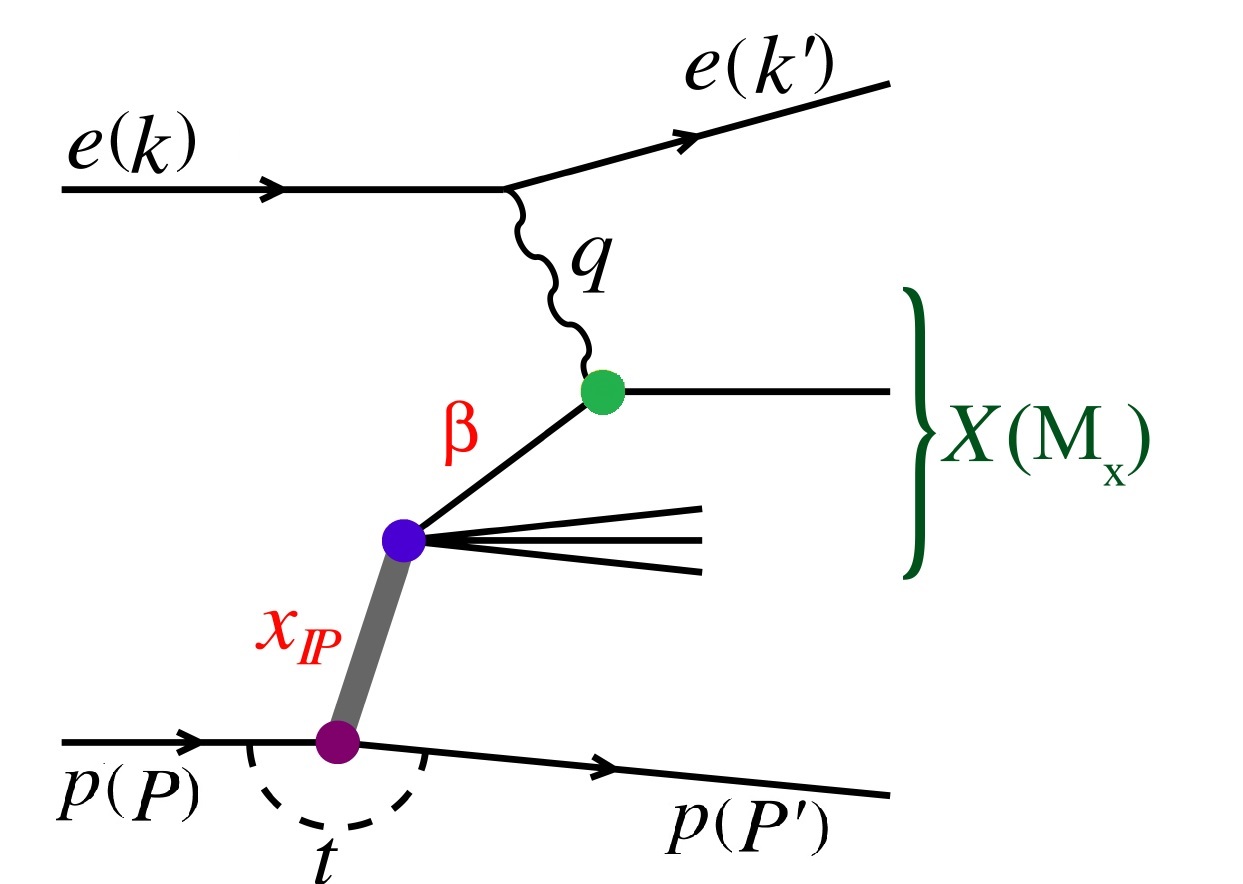
Figure 1: Diagram for diffractive DIS $ep\rightarrow ep{X}$. The four-momenta are indicated as well (in teh round brackets). The diffractive scattered proton is distinguished from the diffractive mass ${X}$.

II.2 Factorization theorem for the diffractive DIS

The main idea of diffractive DIS was proposed for the first time by Ingelman and Schlein Ingelman:1984ns . According to the Ingelman-Schlein (IS) model, the diffractive processes in DIS are interpreted in terms of the exchange of the leading Regge trajectory. The diffractive process includes two steps which are the emission of the pomeron from a proton and subsequent hard scattering of a virtual photon on partons in the pomeron. Therefore the pomeron is considered to have a partonic structure as do hadrons. Hence, the diffractive structure functions factorizes into a pomeron flux and a pomeron structure function Collins:1996fb ; Collins:2001ga ; Collins:1997sr . In analogy to the inclusive DIS, the diffractive structure functions can be written as a convolution of the non-perturbative diffractive PDFs which satisfy the standard DGLAP evolution equations Dokshitzer:1977sg ; Gribov:1972ri ; Lipatov:1974qm ; Altarelli:1977zs , and the hard scattering coefficient functions. It is given by,

$$F {}_{2/L}^{D(4)}({\beta},Q^{2};x_{I\!\!P},{t})=$$

$$\sum_{i}\int_{\beta}^{1}\frac{dz}{z}{C}_{{2}/{L},i}\left(\frac{{\beta}}{z}\right){f}_{i}^{D}(z,Q^{2};{x}_{I\!\!P},{t}),$$ (5)

where the sum runs over all parton flavors (gluon, $d$-quark, $u$-quark, etc.).

Here the long-distance quantity $f_{i}^{D}(z,Q^{2};x_{I\!\!P},{t})$ denotes the non-perturbative part which can be determined by a global QCD analysis of the available diffractive experimental data sets. The Wilson coefficient functions $C_{{2}/{L},{i}}$ in the above equation describe the hard scattering of the virtual photon on a parton ${i}$ and are the same as the coefficient functions known from the inclusive DIS and calculable in perturbative QCD Vermaseren:2005qc . It has been shown that the description of the experimental data is very good when factorization is assumed H1:2006zyl ; ZEUS:2009uxs ; Goharipour:2018yov . The vertex factorization states that the diffractive PDFs should be factorized into the product of two terms, one of them depends on the $x_{I\!\!P}$ and $t$, and the another one is a function of ${\beta}$ and $Q^{2}$. Hence, the diffractive PDFs $f_{i/p}^{D}({\beta},Q^{2};x_{I\!\!P},{t})$ is given by,

$$f_{i/p}^{D}({\beta},Q^{2};x_{I\!\!P},{t})= f_{I\!\!P/p}(x_{I\!\!P},{t})f_{i/I\!\!P}({\beta},Q^{2})$$

$$+ f_{I\!\!R/p}(x_{I\!\!P},{t})f_{i/I\!\!R}^{I\!\!R}({\beta},Q^{2}),$$ (6)

where $f_{I\!\!P/p}(x_{I\!\!P},{t})$ and $f_{I\!\!R/p}(x_{I\!\!P},{t})$ are the Pomeron and Reggeon flux-factors, respectively. These describe the emission of the Pomeron and Reggeon from the proton target. The Pomeron and Reggeon partonic structures given by the parton distributions $f_{{i}/I\!\!P}({\beta},{Q}^{2})$ and $f_{i/I\!\!R}^{I\!\!R}({\beta},Q^{2})$. The parametrization and determination of these functions will be discussed in detail in section III.

II.3 Heavy flavour contributions

The study of the heavy quark flavor contributions to the DIS processes enables us to precisely test QCD and the strong interactions. In this respect, their contributions have an important impact on the PDFs Ball:2021leu ; Boroun:2021ckh ; Harland-Lang:2014zoa ; Ball:2022hsh , FFs Salajegheh:2019nea ; Salajegheh:2019ach ; Soleymaninia:2022qjf , and diffractive PDFs Maktoubian:2019ppi ; Khanpour:2019pzq ; Goharipour:2018yov extracted from the global QCD analysis.

Generally speaking, there are two regimes for the treatment of heavy quark production. The first region is $Q^{2}\sim m_{h}^{2}$ where $m_{h}$ is the heavy quark mass. The massive quarks are produced in the final state and they are not treated as an active parton within the nucleon. This regime is interpreted using the “Fixed Flavour Number Scheme” (FFNS). In this scheme, the light quarks are considered to be the active partons inside the nucleon, and the number of flavors needs to be fixed to $n_{f}=3$. The FFNS is not accurate and reliable for scales much greater than the heavy quark mass threshold $m_{h}^{2}$. At higher energy scales, ${Q}^{2}\gg m_{h}^{2}$, the heavy quarks behave as massless partons within the hadron. It that case, logarithmic terms $\sim Q^{2}/m_{h}^{2}$ are automatically summed through the solutions of the DGLAP evolution equations for the heavy quark distributions. The simplest approach which describes the ${Q}^{2}/m_{h}^{2}\rightarrow\infty$ limit is the “Zero Mass Variable Flavor Number Scheme” (ZM-VNS), which ignores all the $\mathcal{O}(m_{h}^{2}/{Q}^{2})$ corrections. In summary, at very large scales, where the resummation of large logarithms are pertinent, the ZM-VFNS would be more precise, and in the limits close to the heavy quark mass threshold ${m}_{h}$, the FFNS works well enough. In order to present the correct scheme and to obtain the best description of these two limits of $Q^{2}\leq m_{h}^{2}$ and $Q^{2}\gg m_{h}^{2}$, one needs to take into account the “General Mass Variable Flavor Number Scheme” (GM-VFNS) Thorne:2012az . In this scheme, the DIS structure function can be written as follows,

$$F(x,Q^{2})=C_{j}^{{\text{GMVFN}},n_{f}+m}(Q^{2}/m_{h}^{2})\otimes f_{j}^{n_{f}+{m}}(Q^{2}),$$ (7)

where ${n}_{f}$ is the number of active light quark flavors and ${m}$ is the number of heavy quarks. Unlike the ZM-VFNS, the hard scattering coefficient functions ${C}_{k}^{{\text{FF}},n_{f}}$ depend on the $(Q^{2}/m_{h}^{2})$ but reduce to the zero mass approach as $Q^{2}/m_{h}^{2}\rightarrow\infty$. Considering the transition from ${n}_{f}$ active quarks to ${n}_{f}+1$ ones, one could write,

$$F(x,{Q}^{2})= {C}_{j}^{{\text{GMVFN}},n_{f}+1}(Q^{2}/m_{h}^{2})\otimes f_{j}^{n_{f}+1}(Q^{2})$$

$$= C_{j}^{{\text{GMVFN}},n_{f}+{1}}(Q^{2}/m_{h}^{2})\otimes A_{jk}(Q^{2}/m_{h}^{2})$$

$$\qquad\qquad\qquad\qquad\quad\quad\otimes{f}_{k}^{n_{f}}(Q^{2})$$

$$\equiv C_{k}^{FF,{n}_{f}}(Q^{2}/{m}_{h}^{2})\otimes f_{k}^{n_{f}}(Q^{2}),$$ (8)

where the matrix elements $A_{jk}(Q^{2}/m_{h}^{2})$ are calculated and presented in Ref. Buza:1996wv . The $C_{k}^{{\text{FF}},{n}_{f}}(Q^{2}/m_{h}^{2})$ coefficient in the above equation is given by,

$$C_{k}^{{\text{FF}},n_{f}}(Q^{2}/m_{h}^{2})\equiv A_{jk}(Q^{2}/m_{h}^{2})\otimes f_{k}^{n_{f}}(Q^{2}).$$ (9)

As we mentioned before, the coefficient functions must behave towards the massless limit as ${Q}^{2}/m_{h}^{2}\rightarrow{\infty}$, as given by Eq. (9). The analysis presented in this work is based on the Thorne and Roberts (TR) GM-VFNS which covers smoothly from FFNS scheme at low ${Q}^{2}$ to the ZM-VFNS descritption at high energy scale ${Q}^{2}$, and in this regard, our choice gives the best description of the heavy flavor effects on the diffractive structure functions. In this study, following the MMHT14 collaboration, we adopt the values for heavy quarks as ${m}_{c}=1.40\,$GeV and ${m}_{b}=4.75\,$GeV Harland-Lang:2015qea . The strong coupling constant is fixed to ${\alpha}_{s}(M_{Z}^{2})=0.1185$ ParticleDataGroup:2018ovx .

II.4 Twist-4 correction

In this section, we describe in detail the twist-4 correction considered in the SKMHS22 QCD analysis. Generally speaking, the higher twist contribution is proportional to the terms depending on ${1}/Q^{2}$, and hence, would be highly suppressed at a high-energy scale ${Q}^{2}$ in the DIS process. Nonetheless, in the color dipole framework this term for ${M}\rightarrow 0$ or ${\beta}\rightarrow{1}$ dominates over the twist-2 contribution. Hence, the dipole picture provides a powerful framework in which the QCD-based saturation models can be used to investigate the diffractive DIS data.

For interaction of the color dipole with a proton, one could consider two different models which are the quark dipole (${q}\bar{q}$ system) and gluon dipole (${q}\bar{q}g$) system. We refer the reader to the Ref. Golec-Biernat:2008mko for a clear review.

As we mentioned earlier, for the diffractive cross-section, the virtual photon could be transversely or longitudinally polarized. Therefore, according to the different polarization, one can decompose it into a transverse and a longitudinal part. It turns out for the leading order in ${Q}^{2}$ for ${\beta}\rightarrow{1}$, the ${q}\bar{q}$ and ${q}\bar{q}g$ from transverse virtual photons vanish proportional to the $({1}-{\beta})$, whereas the longitudinal part which is of higher twist and gives a finite contribution. In diffractive DIS, for ${M}\ll{Q}^{2}$, the ${q}\bar{q}$ contribution to the final state dominates over ${q}\bar{q}{g}$ of the photon wave function. Thus, the ${L}{q}\bar{q}$ component is not negligible at higher value of ${\beta}$ and has an important contribution in the longitudinal diffractive structure function. The ${F}_{Lq\bar{q}}^{D}$ can be written in term of the Bessel functions ${J}_{0}$ and ${K}_{0}$ and dipole cross section $\hat{\sigma}({x}_{I\!\!P},{r})$ Golec-Biernat:2007mao ; Golec-Biernat:2008mko ,

$$F_{Lq\bar{q}}^{D}= \frac{3}{16{\pi}^{4}x_{I\!\!P}}e^{-B_{D}|t|}\sum_{f}e_{f}^{2}\frac{{\beta}^{3}}{({1}-{\beta})^{4}}$$

$$\times\int_{0}^{[Q^{2}(1-{\beta})]/{4}{{\beta}}}dk^{2}\frac{k^{2}/Q^{2}}{\sqrt{{1}-\frac{{4}{\beta}}{{1}-{\beta}}\frac{k^{2}}{Q^{2}}}}$$

$$\times\left(k^{2}\int_{0}^{\infty}drr{K}_{0}\left(\sqrt{\frac{{\beta}}{{1}-{\beta}}}kr\right){J}_{0}(kr)\hat{\sigma}({x}_{I\!\!P},{r})\right)^{2}\,.$$ (10)

The main idea for the dipole approach is that the photon splits up into a quark-antiquark pair (dipole), which then scatters on the proton target. Following the studies presented in Refs. Golec-Biernat:1998zce , the dipole cross-section is considered to have the following simple form in our QCD analysis,

$$\hat{\sigma}({x}_{I\!\!P},{r})=\sigma_{0}\{{1}-\exp(-r^{2}{Q}_{s}^{2}/{4})\},$$ (11)

where ${r}$ indicates the separation between the quark and the antiquark. The saturation momentum $Q_{s}^{2}=(x_{I\!\!P}/x_{0})^{-\lambda}$ GeV² is responsible for the transition to the saturation regime. The parameters $\sigma_{0}=29$ mb, $x_{0}=4\times 10^{-5}$, and $\lambda=0.28$ are taken from Ref. Golec-Biernat:1998zce . This definition of the dipole-proton cross-section presents a good description of the inclusive HERA diffractive DIS data sets. Our QCD analysis which includes the twist-4 correction is called SKMHS22-tw2-tw4. The effect of such corrections on the extracted diffractive PDFs is discussed in section. IV.

II.5 Reggeon contribution

For the higher value of ${x}_{I\!\!P}$, these diffractive DIS data sets include the contributions which decrease with energy. In order to truly describe this effect one can include the contributions of the subleading Reggeon which breaks the factorization of the diffractive structure function. In order to take into account such contributions, we add the following Reggeon contribution to the diffractive structure function $F^{2}_{D}$ Golec-Biernat:1996bax ; Golec-Biernat:1997vbr

$$\frac{dF_{2}^{R}}{d{x}_{I\!\!P}dt}({x},Q^{2},x_{I\!\!P},{t})=f^{R}(x_{I\!\!P},{t})\,F_{2}^{R}({\beta},{Q}^{2})\,,$$ (12)

where the ${f}^{R}(x_{I\!\!P},{t})$ is the Reggeon flux, and the ${F}_{2}^{R}({\beta},Q^{2})$ is the Reggeon structure function. In principle, we should consider different Regge pole contributions and sum over them and include interference terms. Approximately, one can neglect the interference terms between Reggeons and the Pomeron and also between different Reggeons. Therefore for the Reggeon flux, we consider the following formulas:

$$f^{R}({x}_{I\!\!P},{t})=\sum_{R_{i}}f^{R_{i}}(x_{I\!\!P},{t})\,,$$ (13)

and

$$f^{R_{i}}(x_{I\!\!P},{t})=\frac{F^{2}_{i}(0)}{{8}\pi}e^{-|t|/{\lambda}_{i}^{2}}{C}_{i}(t){x}_{I\!\!P}^{{1}-{2}\alpha_{i}(t)}\,.$$ (14)

Here, $C_{i}(t)={4}\cos^{2}[\pi{\alpha}_{i}(t)/2]$ and $C_{i}(t)={4}\sin^{2}[\pi{\alpha}_{i}(t)/2]$ are the signature factors for the even Reggeon ($f_{2}$) and the odd Reggeon (${\omega}$), respectively. The Reggeon trajectory is given by ${\alpha}_{i}(t)=0.5475+(1.0$ GeV${}^{-2})t$. From Ref. Golec-Biernat:1997vbr , $F^{2}_{f_{2}}(0)=194$ GeV^-2 and $F^{2}_{\omega}(0)=52$ GeV^-2 which denote the Reggeon couplings to the proton. $\lambda_{i}^{2}=0.65$ GeV is known from Reggeon phenomenology in hadronic reactions. The analysis for the isoscalar Reggeons $f_{2},{\omega}$ shows that the Reggeon contribution to the diffractive structure-function becomes important for ${x}_{I\!\!P}>0.01$ H1:2006uea . Our assumption for the Reggeon structure functions is that they are the same for all Reggeons and ${F}_{2}^{R}({\beta},{Q}^{2})$ is related to the parton distributions in the Reggeons in a conventional way and can be determined by the fit to diffractive DIS data from HERA H1:2012xlc ; H1:2012pbl ; H1:2011jpo . For the Reggeon structure-function, we consider the following parametrization form,

$${F}_{2}^{R}({\beta})=w_{1}{\beta}^{w_{2}}(1-{\beta})^{w_{3}}(1+w_{4}\sqrt{{\beta}}+w_{5}{\beta}^{2})\leavevmode\nobreak\ ,$$ (15)

where $w_{1}$, $w_{2}$, $w_{3}$ and $w_{4}$ are free fit parameters and they need to be determined from a global QCD analysis. The parameter $w_{2}$ controls the shape of $F_{2}^{R}({\beta})$ in the low-$\beta$ region, while $w_{3}$ controls the high-$\beta$ region. The parameters $w_{4}$ and $w_{5}$ are considered to be fixed to zero, as the current diffractive DIS data sets do not have enough power to constrain all the shape parameters. Our QCD analysis which includes the Reggeon contribution is called SKMHS22-tw2-tw4-RC, and the effect arising from the inclusion of such correction is discussed in section. IV.

III Diffractive PDFs global QCD analysis details

The analysis of diffractive PDFs is a QCD optimization problem and can be seen as having four elements to it. The first and most important element is of course the experimental data and their uncertainty. The second element is a theoretical model used to describe these phenomenon. For the analysis of non-perturbative objects such as diffractive PDFs this theoretical framework can have some adjustable parameters as well as a number of constraints (say for ensuring of factorization). Another part of the problem is the objective function which we wish to minimize/maximize. Here, this function is a $\chi^{2}$ function that is defined by the theoretical framework and includes the data uncertainty. The last part of the problem is the optimization method which is the essential step to finding the solution.

In this section, we present the methodology of our global QCD analysis to obtain the diffractive PDFs and their uncertainties at NLO accuracy in perturbative QCD. We describe the details of the data sets used for the following fit in section III.1 , the parametrization of diffractive PDFs is discussed in section III.2, and the methodology of minimization and uncertainties of our diffractive PDFs are described in section III.3.

III.1 Experimental data sets

Table 1: List of all diffractive DIS data points with their properties used in the SKMHS22 global QCD analysis. For each data set we provide the kinematical coverage of ${\beta}$, ${{x}_{I\!\!P}}$, and ${Q}^{2}$. The number of data points is displayed as well. The details of the kinematical cuts applied on these data sets are explained in the text.

Experiment	Observable	[$\beta^{{\text{min}}},{\beta}^{{\text{max}}}$]	[${x_{I\!\!P}}^{\rm{min}},{x_{I\!\!P}}^{\rm{max}}$]	${Q}^{2}\,[{\text{GeV}}^{2}]$	# of points	Reference
H1-LRG-11 $\sqrt{s}={225}$ GeV	${\sigma}_{r}^{D(3)}$	[$0.033$–$0.88$]	[$5{\times}10^{-4}$ – $3{\times}10^{-3}$]	4–44	22	H1:2011jpo
H1-LRG-11 $\sqrt{s}={252}$ GeV	${\sigma}_{r}^{D(3)}$	[$0.033$–$0.88$]	[$5{\times}10^{-4}$ – $3{\times}10^{-3}$]	4–44	21	H1:2011jpo
H1-LRG-11 $\sqrt{s}={319}$ GeV	${\sigma}_{r}^{D(3)}$	[$0.089$–$0.88$]	[$5{\times}10^{-4}$ – $3{\times}10^{-3}$]	11.5–44	14	H1:2011jpo
H1-LRG-12	${\sigma}_{r}^{D(3)}$	[$0.0017$–$0.80$]	[$3{\times}10^{-4}$ – $3{\times}10^{-2}$]	3.5–1600	277	H1:2012pbl
H1/ZEUS combined	${\sigma}_{r}^{D(3)}$	[$0.0018$–$0.816$]	[$3{\times}10^{-4}$ – $9{\times}10^{-2}$]	2.5–200	192	H1:2012xlc
Total data					526

In this section, we describe all available inclusive diffractive DIS data sets in detail. However, one needs to apply some kinematical cuts in order to avoid nonperturbative effects and ensure that only the data sets for which the available perturbative QCD treatment is adequate are included in the QCD analysis. We attempt to include more data sets, and hopefully by including the twist-4 and Reggeon contributions, one could relax some kinematical cuts that need to be applied to the data.

The kinematic coverage in the (${\beta}$, ${x_{I\!\!P}}$, Q²) plane of the complete SKMHS22 data set is displayed in Fig. 2. The data points are classified by different experiments at HERA. As customary, some kinematic cuts need to be applied to the diffractive DIS cross-section measurements.

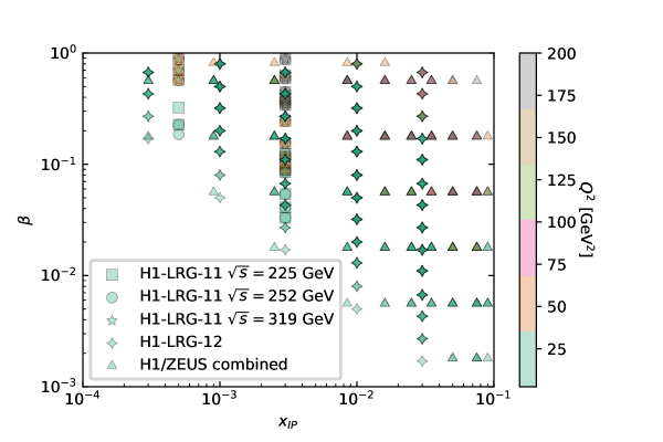
Figure 2: The kinematic coverage in the ($\beta$, ${x_{I\!\!P}}$, Q²) plane of the SKMHS22 data set. The data points are classified by different experiments at HERA.

The list of diffractive DIS data sets and their properties used in the SKMHS22 global analysis are shown in Table 1. All the measurements are presented in terms of the $t$-integrated reduced diffractive DIS cross-section measurements ${D}_{r}^{D(3)}(ep\rightarrow ep{X})$. In the SKMHS22 QCD analysis, we also analyze the combined measurement of the inclusive diffractive cross-section presented by the H1 and ZEUS Collaborations at HERA (H1/ZEUS combined) H1:2012xlc . They used samples of diffractive DIS $ep$ data at the center-of-mass energy of $\sqrt{s}={318}$ GeV at the HERA collider where the leading protons are detected by appropriative spectrometers. This high-precision measurement combined all the previous H1 FPS HERA I H1:2006uea , H1 FPS HERA II Aaron:2010aa , ZEUS LPS 1 ZEUS:2004luu , and ZEUS LPS 2 ZEUS:2008xhs data sets. These measurements cover the photon virtuality interval $2.5<{Q}^{2}<200$ GeV², $3.5{\times}10^{-4}<{x_{I\!\!P}}<0.09$ in proton fractional momentum loss, $0.09<|t|<0.55$ Gev² in squared four-momentum transfer at the proton vertex and $1.8{\times}10^{-3}<{\beta}<0.816$. We should highlight here that all H1-LRG data are published for the range of $|t|<1$ GeV², while the recent combined H1/ZEUS data sets are restricted to the range of $0.09<|t|<0.55$ GeV², and hence, one needs to use a global normalization factor to extrapolate from $0.09<|t|<0.55$ GeV² to $|t|<1$ GeV² Goharipour:2018yov . Therefore, the combined H1/ZEUS data are corrected for the region of $|t|<1$ GeV².

Another data set that we have used in our QCD analysis is the Large Rapidity Gap (LRG) data from H1-LRG-11, which was measured by the H1 detector in 2006 and 2007. These data are derived for three different center of mass energies of $\sqrt{s}={225}$, ${252}$ and ${319}$ GeV H1:2011jpo . The H1 collaboration measured the reduced cross-section in the photon virtualities range $4\,$GeV${}^{2}{\leq}Q^{2}{\leq}44\,$GeV² for the center of mass $\sqrt{s}={225}$, ${252}$ GeV, and $11.5$ GeV${}^{2}{\leq}Q^{2}{\leq}44$ GeV² for the center-of-mass energy of $\sqrt{s}={319}$ GeV. The diffractive final state masses and the proton vertex are in the range of $1.25<{M}_{X}<10.84$ GeV and $|t|<1$ GeV², respectively. The diffractive variables are considered in the range of $5{\times}10^{-4}<{x_{I\!\!P}}<3{\times}10^{-3}$, $0.033<{\beta}<0.88$ for $\sqrt{s}=225$, $252$ GeV, and $0.089<{\beta}<0.88$ for $\sqrt{s}=319$ GeV.

Finally the last data set that we have employed is the H1-LRG-12 H1:2012pbl . These data for the process $ep\rightarrow e{X}{Y}$ have been derived by the H1 experiment at HERA. H1-LRG-12 data covers the range of $3.5<{Q}^{2}<1600\,$GeV², $0.0003\leq{x_{I\!\!P}}\leq 0.03$, and $0.0017{\leq}{\beta}{\leq}0.8$.

We applied some kinematical cuts on ${\beta}$, $M_{X}$, and $Q^{2}$. The kinematical cuts we applied are similar to those used in Refs. Goharipour:2018yov ; ZEUS:2009uxs , except for the case of ${\beta}$. By considering the twist-4 and Reggeon corrections, we can relax the cuts to include more data sets than those have been used in Ref. Goharipour:2018yov . For the extraction of diffractive PDFs we apply $\beta\leq 0.90$ and ${M}_{X}<2$ GeV over all data sets used in this analysis. The sensitivity of data sets to the ${Q}^{2}$ has been tested in Refs. Goharipour:2018yov ; ZEUS:2009uxs . The authors finalized the cut on $Q^{2}$ by making a $\chi^{2}$ scan. In Ref. Maktoubian:2019ppi the authors used standard higher twist for structure functions and they obtained the best $\chi^{2}$ by considering the $Q^{2}_{\text{min}}=6.5$ GeV², and in Ref. Goharipour:2018yov to extract the diffractive PDFs they found the best cut is $Q^{2}_{min}=9$ GeV². In this work and after testing the results for the $\chi^{2}$ we found the best agreement of theory and data will be achieved by taking $Q^{2}_{min}=9$ GeV². After applying these kinematical cuts the total number of data points is reduced to the 302.

III.2 SKMHS22 Diffractive PDFs parametrization form

Diffractive PDFs are nonperturbative quantities and cannot be calculated in perturbative QCD. Therefore, for their functional dependence a parametric form with some unknown parameters should be considered at the input scale. Due the lack of diffractive DIS experimental data, for the quark distributions we consider all light quarks and anti-quarks densities to be equal, ${f}_{u}={f}_{d}={f}_{s}=f_{\bar{u}}=f_{\bar{d}}=f_{\bar{s}}$. The scale dependence of the quarks and gluon distributions ${f}_{q,g}({\beta},{Q}^{2})$ needs to be determined by the standard DGLAP evolution equations. We fit the diffractive quark and gluon distributions at the starting scale ${Q}_{0}^{2}={1.8}$ GeV² which is below the charm threshold ($m_{c}^{2}=1.96$ GeV²). Since the diffractive DIS data sets can only constrain the sum of the diffractive PDFs and due to the small amount of the inclusive diffractive DIS data sets, one needs to consider the less flexible parametrization form for diffractive PDFs.

We fit the diffractive parton distribution function at the initial scale $Q_{0}^{2}=1.8$ GeV² with the following pomeron parton distributions which have been used in several analysis Goharipour:2018yov ; Maktoubian:2019ppi ; H1:2006zyl :

$$zf_{q}(z,{Q}_{0}^{2})= {\alpha}_{q}z^{{\beta}_{q}}({1}-{z})^{{\gamma}_{q}}({1}+{\eta}_{q}\sqrt{z}+{\xi}_{q}z^{2}),$$ (16)

$$zf_{g}(z,{Q}_{0}^{2})= \alpha_{g}z^{{\beta}_{g}}(1-{z})^{{\gamma}_{g}}({1}+{\eta}_{g}\sqrt{z}+{\xi}_{g}z^{2}),$$ (17)

where ${z}$ in above equation is the longitudinal momentum fraction of struck parton with respect to the diffractive exchange. At the lowest order, $z={\beta}$ but by including the higher orders this parameter differs from ${\beta}$ and this leads to the ${0}<{\beta}<{z}$. In order to let the parameters ${\gamma}_{q}$ and ${\gamma}_{g}$ have enough freedom to achieve negative or positive values in the QCD fit we follow the QCD analyses avalible in the litrature and add an additional term ${e}^{-\frac{0.001}{{1}-{z}}}$ to ensure that the distributions vanish for ${z}\rightarrow{1}$. It turned out that four parameters ${\eta}_{q}$, ${\eta}_{g}$, ${\xi}_{q}$ and ${\xi}_{g}$ are not well constrained by the experimental data, and hence, one needs to set them to zero. The heavy flavors are generated through the DGLAP evolution equations at the scale ${Q}^{2}>m_{c,b}$. As we mentioned, to consider the contributions of heavy flavors, we apply the Thorne-Roberts scheme GM-VFN scheme.

The $x_{I\!\!P}$ dependence of the diffractive PDFs $f_{i}^{D}({\beta},Q^{2};x_{I\!\!P},{t})$ in Eq. II.2 is determined by the Pomeron and Reggeon flux with linear trajectories, $\alpha_{{I\!\!P},{I\!\!R}}(0)+\alpha^{\prime}_{{I\!\!P},{I\!\!R}}t$ Goharipour:2018yov ; Maktoubian:2019ppi ; H1:2006zyl

$${f}_{{I\!\!P},{I\!\!R}}({x}_{I\!\!P},t)={A}_{{I\!\!P},{I\!\!R}}\frac{e^{B_{{I\!\!P},{I\!\!R}}}t}{{x}_{I\!\!P}^{{2}\alpha_{{I\!\!P},{I\!\!R}}(t)-{1}}},$$ (18)

where the normalization factor of Reggeon ${A}_{I\!\!R}$ and the Pomeron and Reggeon intercepts, ${\alpha}_{I\!\!P}(0)$ and ${\alpha}_{I\!\!R}(0)$ are free parameters and will be determined from fit to the diffractive DIS data. We should note here that, according to Eq (II.2) the parameter ${A}_{I\!\!P}$ is absorbed into the ${\alpha}_{q}$ and ${\alpha}_{g}$. The remaining parameter appearing in Eq. (18) are taken from Goharipour:2018yov . In general we have twelve free fit parameters: six from Eq. (16) and (17), three form Eq. (18), and three from the Reggeon structure function in Eq. (15).

III.3 Minimization and diffractive PDF uncertainty method

In this section, we present two important parts of the SKMHS22 QCD analysis. First, we discuss the optimization method, and then we show how to take into account the data uncertainty in the final results. In order to estimate the free parameters of the diffractive PDFs given the experimental data of section III.1 we apply the maximum log-likelihood method. If we assume that the data arise from a Gaussian distribution as is usually done, this method coincides with minimizing the $\chi^{2}$ estimator. Here we adopt the following form for the $\chi^{2}$ function H1:2012qti ; Goharipour:2018yov ,

$$\chi^{2}(\{\zeta_{k}\})$$

$$=\displaystyle\sum_{i}\frac{\left[\mathcal{E}_{i}-\mathcal{T}_{i}\left(\{\zeta\}\right)\left(1-\sum_{j}\gamma_{j}^{i}{b}_{j}\right)\right]^{2}}{\delta^{2}_{{i},\mathrm{unc}}\mathcal{T}_{i}^{2}(\{\zeta\})+{\delta}^{2}_{i,\mathrm{stat}}\mathcal{E}_{i}\mathcal{T}_{i}(\{\zeta\})\left(1-\sum_{j}\gamma^{i}_{j}{b}_{k}\right)}$$

$$+\sum_{i}\ln\frac{\delta^{2}_{{i},\mathrm{unc}}\mathcal{T}_{i}^{2}(\{\zeta\})+\delta^{2}_{{i},\mathrm{stat}}\mathcal{E}_{i}\mathcal{T}_{i}(\{\zeta\})}{\delta^{2}_{{i},\mathrm{unc}}\mathcal{E}_{i}^{2}+\delta^{2}_{{i},\mathrm{stat}}\mathcal{E}^{2}_{i}}+\sum_{j}b_{j}^{2}\,,$$ (19)

with $\mathcal{E}$ is the measured experimental value, and $\mathcal{T}$ is the theoretical prediction based on the fit parameters $\{\mathbf{\zeta}_{k}\}$. The parameters ${\delta}_{i,\mathrm{stat}}$ , $\delta_{i,\mathrm{unc}}$, and $\gamma^{i}_{j}$ denote the relative statistical, uncorrelated systematic, and correlated systematic uncertainties, respectively. The nuisance parameters ${b}_{{k}}$ are related to correlated systematic uncertainty and are determined with the $\{\zeta_{k}\}$ parameters simultaneously in the QCD fit.

The above ${\chi}^{2}$ function is incorporated in the xFitter framework, in conjunction with other tools required for a perturbative QCD analysis of diffractive PDFs. One then can use this package to perform all the essential operations such as DGLAP evolution up to NNLO accuracy, theoretical calculation of the relevant observables and finding out optimal parameter values and deducing their uncertainty collectively. As we specified above in order to find the optimal fit parameter values one needs to minimize the ${\chi}^{2}$ function, this is achieved by utilizing the MINUIT CERN package James:1975dr . This package finds the parameter uncertainties by considering the $\chi^{2}$ function around its minimum. MINUIT has five minimization algorithms, here we choose to work with MIGRAD which is the most commonly used method of minimization.

In practice, we need to propagate these parameter uncertainties to the observables or other quantities like the diffractive PDFs themselves. For this aim, a set of eigenvector PDF sets along with the the central values of the diffractive PDFs is formed, for our fit that has 9 free parameters, the total number of PDF sets will be 19. Each member of the error set is derived by either increasing or decreasing one of the parameters by its uncertainty. Then, the uncertainty of a quantity ${\cal O}$ due to its dependence on PDFs is given as in Ref. Nadolsky:2008zw ,

$$\Delta{\cal O}=\frac{1}{2}\sqrt{\sum_{{i}={1}}^{N}\left({\cal O}_{i}^{(+)}-{\cal O}_{i}^{(-)}\right)^{2}}\,,$$ (20)

where ${\cal O}_{i}^{(\pm)}$ refer to the values of ${\cal O}$ which are calculated from PDF sets of the $i$-th parameter along with the $\pm$ directions. In the derivation of this relation, it is assumed that the variation of ${\cal O}$ can be approximated by linear terms of its Taylor series and then the gradient is approximated, which produces the above result. In the next section, we present our main results and findings of the SKMHS22 diffractive PDFs and some observables in order to show the quality of the analysis.

IV Fit results

This section includes the main results of the SKMHS22 diffractive PDFs analysis. As we discussed in detail earlier, in this QCD analysis we present three different QCD fits to determine the diffractive PDFs which are SKMHS22-tw2, SKMHS22-tw2-tw4 and SKMHS22-tw2-tw4-RC. In this section we will present and discuss these results in turn. The similarity and difference of these results over different kinematical ranges will be highlighted, and the stability of the results upon the inclusion of higher-twist corrections will be discussed in detail. This section also includes a detailed comparison with the diffractive DIS data analyzed in this work.

The best fit parameters for three sets of SKMHS22 diffractive PDFs are shown in Table 2 along with their experimental errors. Considering the numbers presented in this table, some comments are in order. The parameters $\eta_{g}$ and $\eta_{q}$ are considered to be fixed at zero as the present diffractive DIS data sets do not have enough power to constrain all shape parameters of the distributions.

The parameter {$w_{i}$} for the Reggeon structure function for the SKMHS22-tw2-tw4-RC analysis presented in Eq. 15 are determined along the fit parameters and then keep fixed to their best fitted values. The parameters $w_{4}$ and $w_{5}$ are keep fixed at zero. The values for the strong coupling constant $\alpha_{s}(M_{Z}^{2})$ and the charm and bottom quark masses also are shown in the table as well.

Table 2: Best fit parameters obtained with the SKMHS22-tw2, SKMHS22-tw2-tw4 and SKMHS22-tw2-tw4-RC fits at the initial scale of $Q_{0}^{2}=1.8\,{\text{GeV}}^{2}$ along with their experimental uncertainties. The values marked with the (*) are fixed in the fit.

Parameters	SKMHS22-tw2	SKMHS22-tw2-tw4	SKMHS22-tw2-tw4-RC
$\alpha_{g}$	$1.00\pm 0.16$	$1.07\pm 0.17$	$1.43\pm 0.23$
$\beta_{g}$	$0.226\pm 0.066$	$0.332\pm 0.070$	$0.447\pm 0.070$
$\gamma_{g}$	$0.27\pm 0.15$	$0.19\pm 0.14$	$0.37\pm 0.14$
$\eta_{g}$	$0.0^{*}$	$0.0^{*}$	$0.0^{*}$
$\alpha_{q}$	$0.305\pm 0.022$	$0.517\pm 0.041$	$0.727\pm 0.059$
$\beta_{q}$	$1.474\pm 0.069$	$1.887\pm 0.081$	$2.149\pm 0.0584$
$\gamma_{q}$	$0.509\pm 0.034$	$0.980\pm 0.0948$	$1.137\pm 0.050$
$\eta_{q}$	$0.0^{*}$	$0.0^{*}$	$0.0^{*}$
$\alpha_{I\!\!P}(0)$	$1.0934\pm 0.0032$	$1.1021\pm 0.0037$	$1.0965\pm 0.0037$
$\alpha_{I\!\!R}(0)$	$0.316\pm 0.053$	$0.400\pm 0.053$	$0.418\pm 0.054$
$A_{I\!\!R}$	$21.7\pm 5.7$	$15.0\pm 3.9$	$13.2\pm 3.5$
$w_{1}$	$0.0^{*}$	$0.0^{*}$	$0.23^{*}$
$w_{2}$	$0.0^{*}$	$0.0^{*}$	$3.79^{*}$
$w_{3}$	$0.0^{*}$	$0.0^{*}$	$14.9^{*}$
$w_{4}$	$0.0^{*}$	$0.0^{*}$	$0.0^{*}$
$w_{5}$	$0.0^{*}$	$0.0^{*}$	$0.0^{*}$
$\alpha_{s}(M_{Z}^{2})$	$0.1185^{*}$	$0.1185^{*}$	$0.1185^{*}$
$m_{c}$	$1.40^{*}$	$1.40^{*}$	$1.40^{*}$
$m_{b}$	$4.75^{*}$	$4.75^{*}$	$4.75^{*}$

In the following, we turn our attention to the detailed comparison of the three SKMHS22 diffractive PDFs sets. We display the SKMHS22-tw2, SKMHS22-tw2-tw4 and SKMHS22-tw2-tw4-RC diffractive PDFs parameterized in our QCD fits, Eqs. (16) and (17), along with their uncertainty bands in Fig. 3 at the input scale $Q_{0}^{2}=1.8$ GeV². The higher Q² value results at 6 and 20 GeV² are shown in Figs. 4 and Fig. 5, respectively. The lower panels show the ratio of SKMHS22-tw2-tw4 and SKMHS22-tw2-tw4-RC to the SKMHS22-tw2.

In Fig. 6, we display the perturbatively generated SKMHS22 diffractive PDFs for the charm and bottom quark densities along with their error bands at the scale of $Q^{2}=60$ GeV² and 200 GeV². All three diffractive PDFs sets are shown for comparison.

A remarkable feature of the SKMHS22 diffractive gluon and quark PDFs shown in these figures is the difference both in the shape and error bands, which reflects the effect arising from the inclusion of higher twist corrections. As can be seen, for all cases the inclusion of the twist-4 and Reggeon corrections lead to slightly small error bands. This is consistent with the ${\chi^{2}}$ value presented in Table 3. The inclusion of the twist-4 corrections and Reggeon contributions leads to an enhancement of the gluon diffractive PDFs at high $\beta$, and a reduction of the singlet PDFs as well. Considering such corrections also affects the small regions of $\beta$ and leads to the reduction of the central values of all distributions. These findings indicate that for the given kinematical range of the diffractive DIS data from the ZEUS and H1 Collaborations, considering the higher twist corrections is of crucial importance.

For the gluon PDFs, we see a very large error band for a small region of $\beta$, namely $\beta<0.01$, which indicates that the available diffractive DIS data do not have enough power to constrain the low-$\beta$ gluon density. To better constrain the gluon PDFs, the diffractive dijet productions data need to be taken into account H1:2014pjf ; H1:2015okx . In terms of future work, it would be very interesting to repeat the QCD analysis described here to study the impact of diffractive dijet production data on the diffractive gluon PDF and its uncertainty.

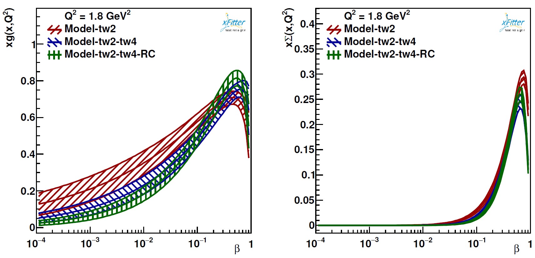
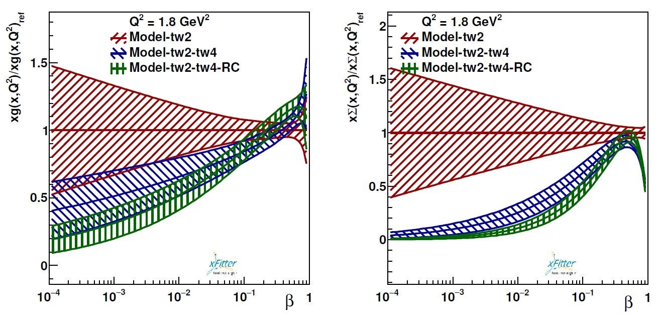
Figure 3: The SKMHS22 diffractive PDFs at the input scale of $Q_{0}^{2}=1.8$ GeV². All three diffractive PDFs sets are shown for comparison. The lower panels represent the ratio of SKMHS22-tw2-tw4 and SKMHS22-tw2-tw4-RC to the SKMHS22-tw2.

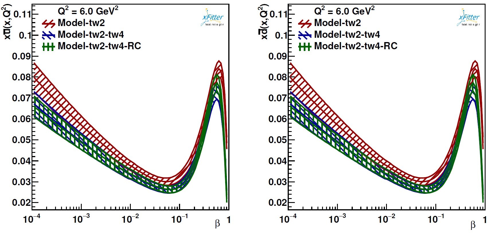
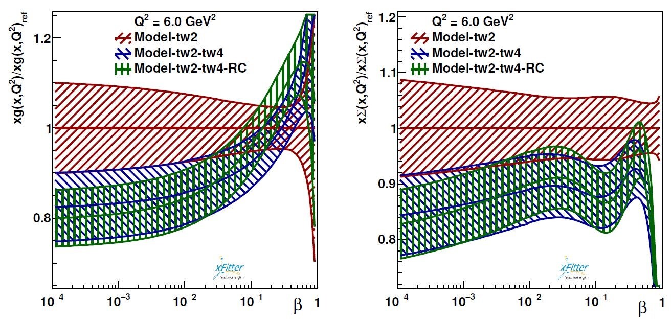
Figure 4: Same as in Fig. 3 but this time for the the higher energy scale of 6 GeV².

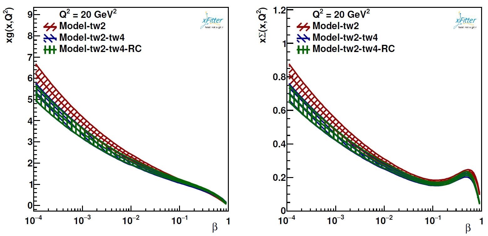
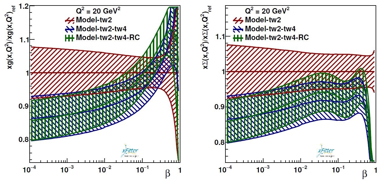
Figure 5: Same as in Fig. 3 but this time for the the higher energy scale of 20 GeV².

The same discussion also holds for the case of heavy quark diffractive PDFs. As one can see from Fig. 6, the SKMHS22-tw2-tw4-RC charm and bottom quark densities lie below other results for all regions of $\beta$.

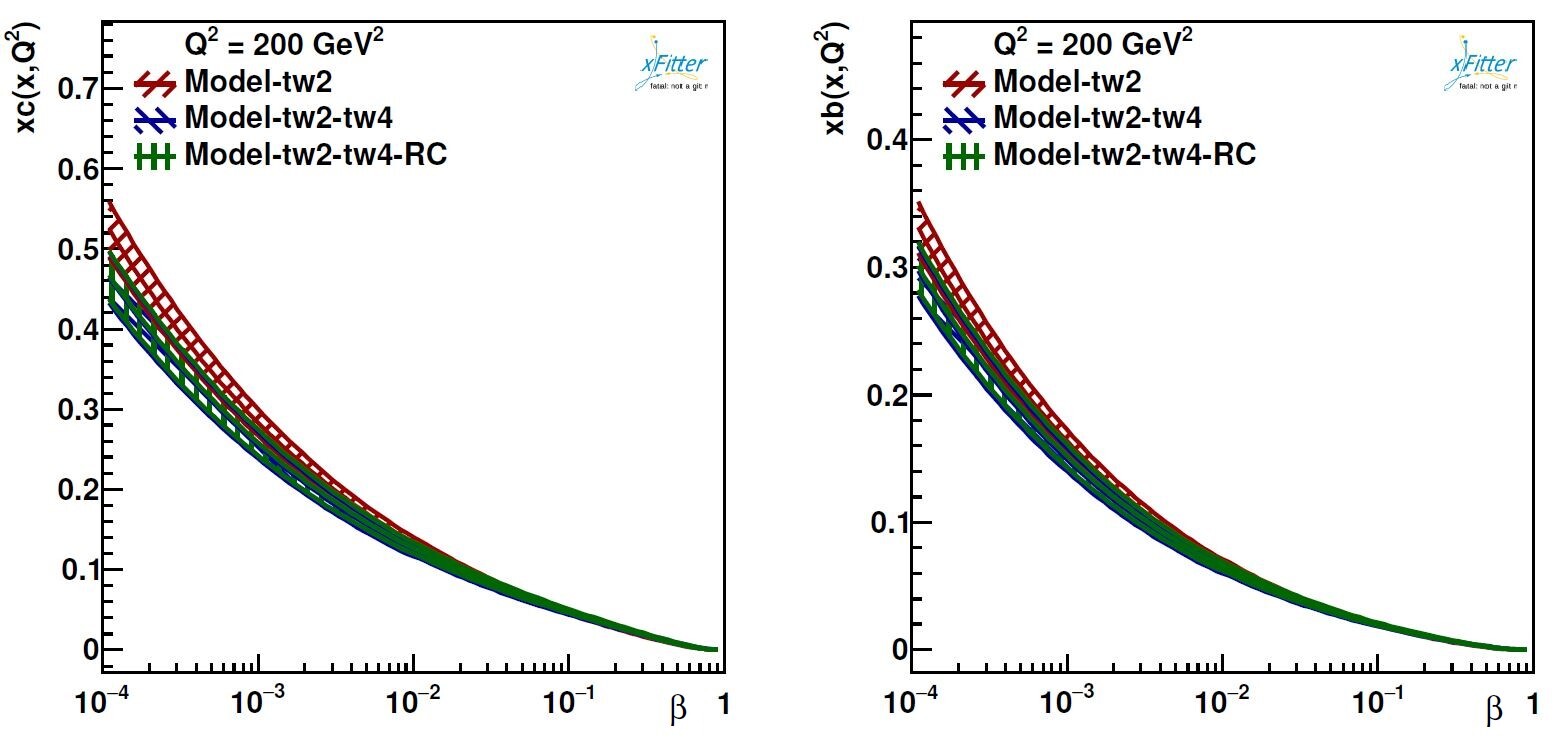
Figure 6: The perturbatively generated SKMHS22 diffractive PDFs for the charm and bottom quark densities along with their error bands at the scale of $Q^{2}=60$ and 200 GeV². All three diffractive PDFs sets are shown for comparison.

In Table. 3, we present the values for the $\chi^{2}$ per data point for both the individual and the total diffractive DIS data sets included in the SKMHS22 analysis. The values are shown for all three sets of SKMHS22-tw2, SKMHS22-tw2-tw4 and SKMHS22-tw2-tw4-RC. Concerning the fit quality of the total diffractive DIS data sets, the most noticeable feature is an improvement in the inclusion of the Reggeon contribution. The improvement of the individual $\chi^{2}$ per data point is particularly pronounced for the H1-LRG 2012 when the Reggeon contribution in considered in the analysis. This finding demonstrates the fact that the inclusion of the higher-twist corrections improves the description of the diffractive DIS data sets.

Table 3: The values of $\chi^{2}/N_{\text{pts}}$ for the data sets included in the SKMHS22 global fits.

	SKMHS22-tw2	SKMHS22-tw2-tw4	SKMHS22-tw2-tw4-RC
Experiment	${\chi}^{2}/{N}_{\text{pts}}$	${\chi}^{2}/{N}_{\text{pts}}$	${\chi}^{2}/{N}_{\text{pts}}$
H1-LRG-11 $\sqrt{s}={225}$ GeV H1:2011jpo	11/13	11/13	12/13
H1-LRG-11 $\sqrt{s}={252}$ GeV H1:2011jpo	20/12	21/12	19/12
H1-LRG-11 $\sqrt{s}={319}$ GeV H1:2011jpo	6.6/12	3.7/12	4.6/12
H1-LRG-12 H1:2012pbl	136/165	143/165	124/165
H1/ZEUS combined H1:2012xlc	129/100	124/100	125/100
Correlated ${\chi}^{2}$	11	16	19
Log penalty ${\chi}^{2}$	+11	+22	+15
${\chi}^{2}/{\text{dof}}$	$\leavevmode\nobreak\ 324/293=1.10\leavevmode\nobreak\$	$\leavevmode\nobreak\ 319/293=1.16\leavevmode\nobreak\$	$\leavevmode\nobreak\ 319/293=1.08\leavevmode\nobreak\$

In order further high-light the SKMHS22 analysis, in the following, we present a detailed comparison of the diffractive DIS data set analyzed in this work to the corresponding NLO theoretical predictions obtained using the NLO diffractive PDFs from all three sets. As we will show, in general, overall good agreements between the diffractive data and the theoretical predictions are achieved for all H1 and ZEUS data.

We start with the comparison to the H1-LRG-11 $\sqrt{s}=225$, 252 and 319 GeV data. In Fig. 7, the SKMHS22 theory predictions are compared with some selected data points. The comparisons are shown as a function of $\beta$ and for selected bins of $x_{I\!\!P}$=0.0005 and 0.003. As one can see, very nice agreement is achieved for all regions of $\beta$

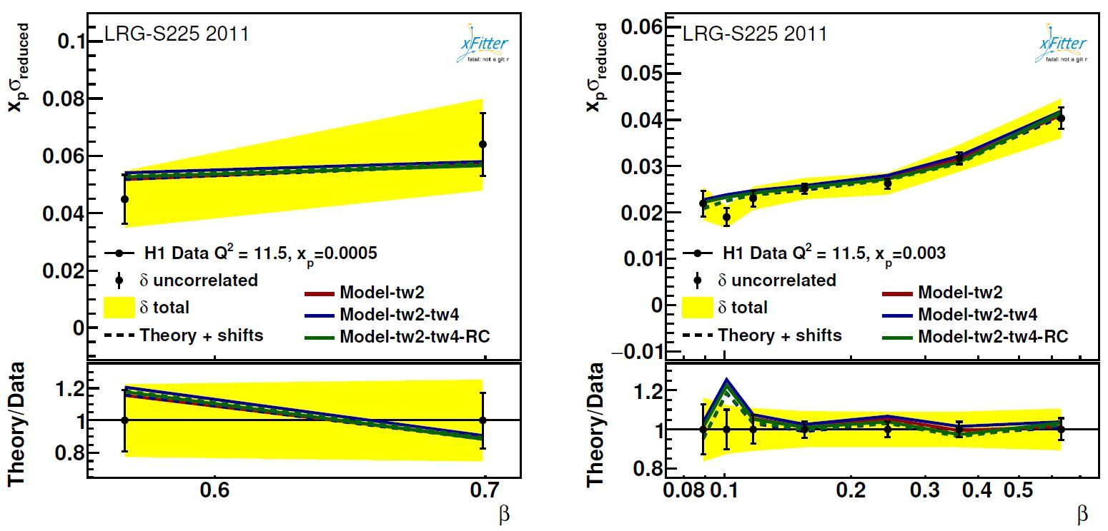
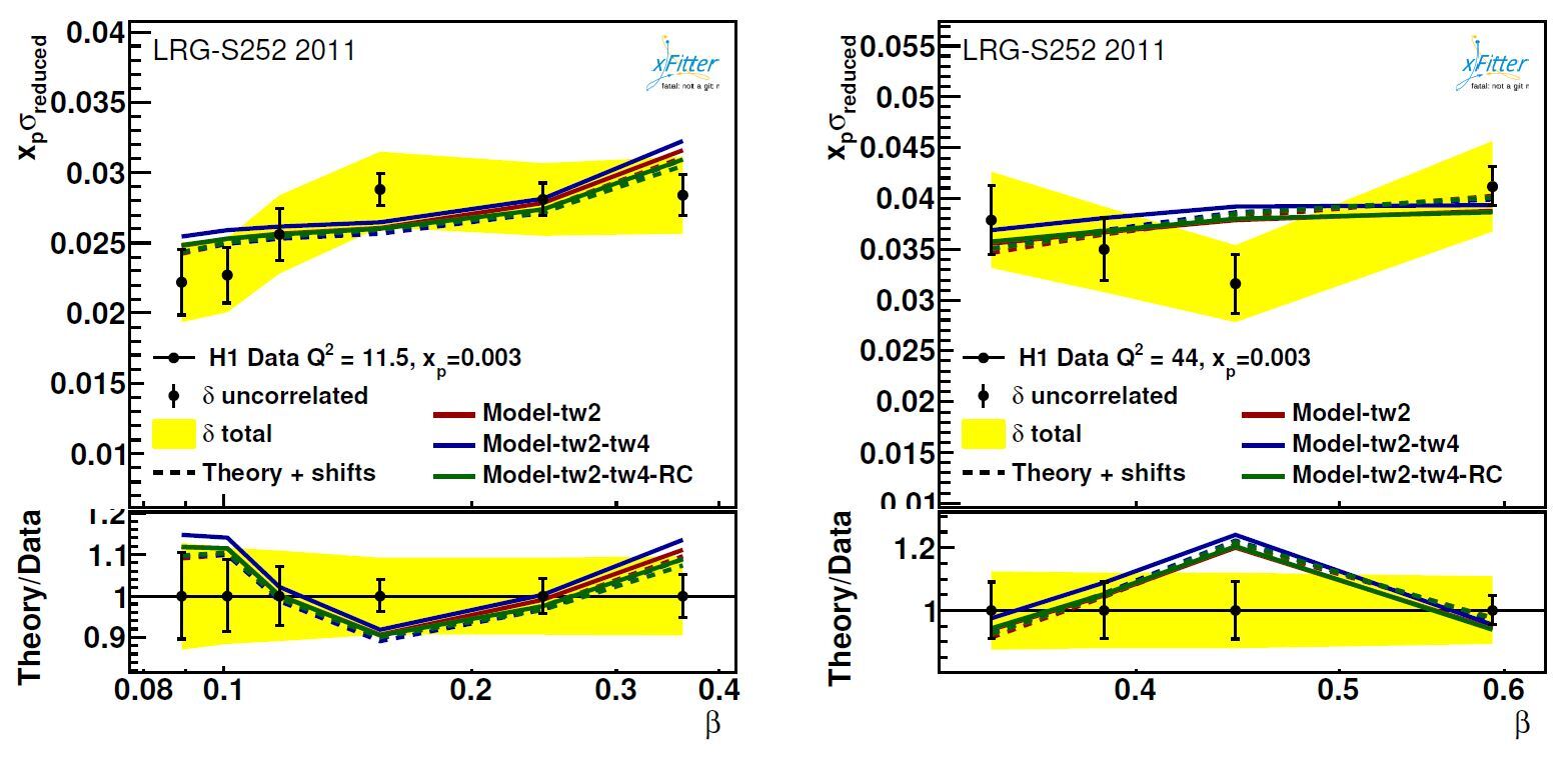
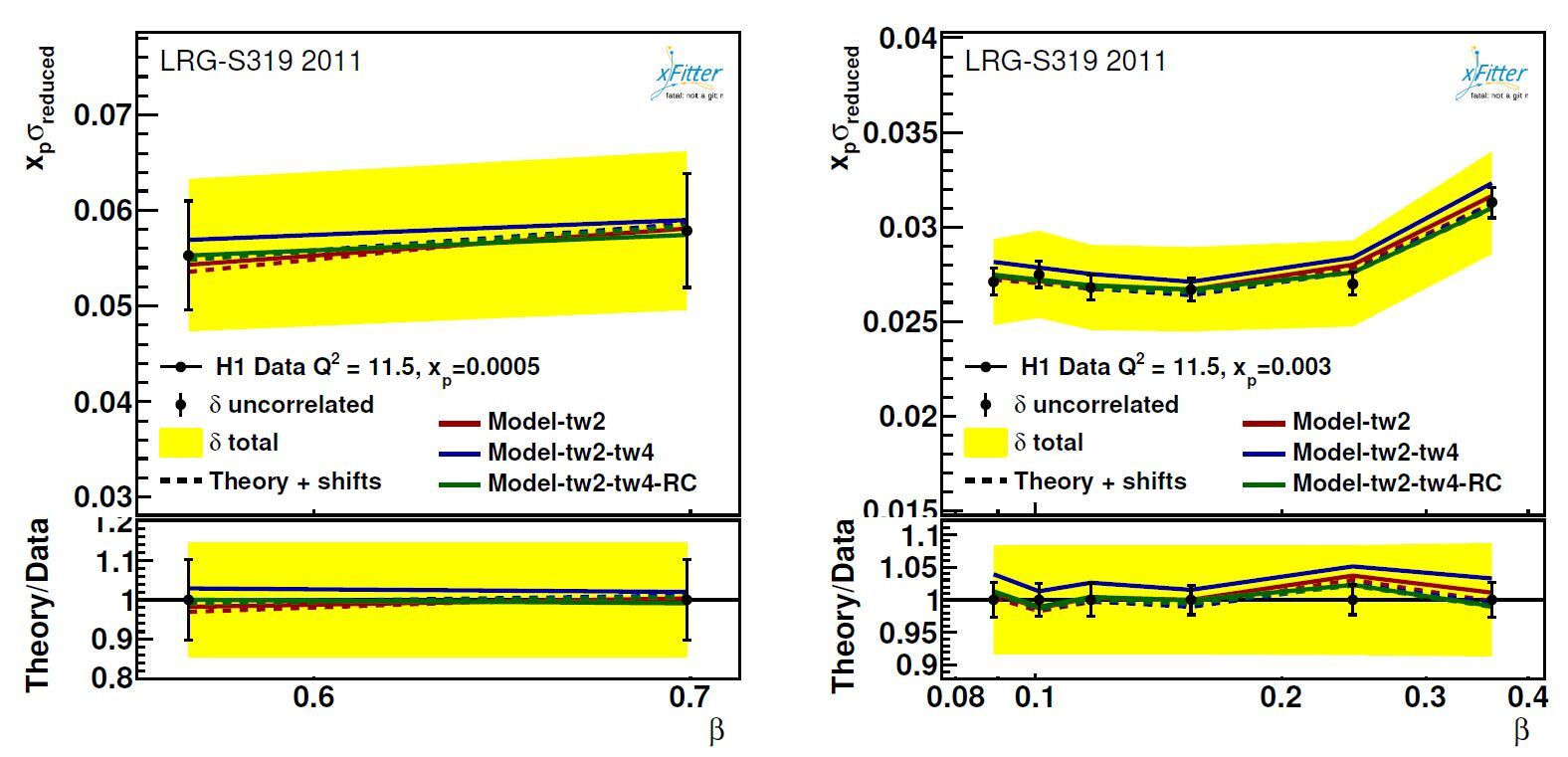
Figure 7: Comparison between the diffractive DIS data set from the H1-LRG-11 $\sqrt{s}=225$, 252 and 329 GeV and the corresponding NLO theoretical predictions using all three diffractive PDFs sets. We show both the absolute distributions and the data/theory ratios.

The same comparisons are also shown in Fig. 8 for the H1-LRG-12 for some selected bins of $x_{I\!\!P}$ namely 0.01, 0.03, and 0.003. In these plots, the SKMHS22 theory precision for all three different sets are compared with the H1-LRG-12 diffractive DIS data. The comparisons are shown as a function of $\beta$ and for different values of Q². As one can see, very good agreements between the data and theory predictions are achieved, consistent with the total and individual $\chi^{2}$ presented in Table 3.

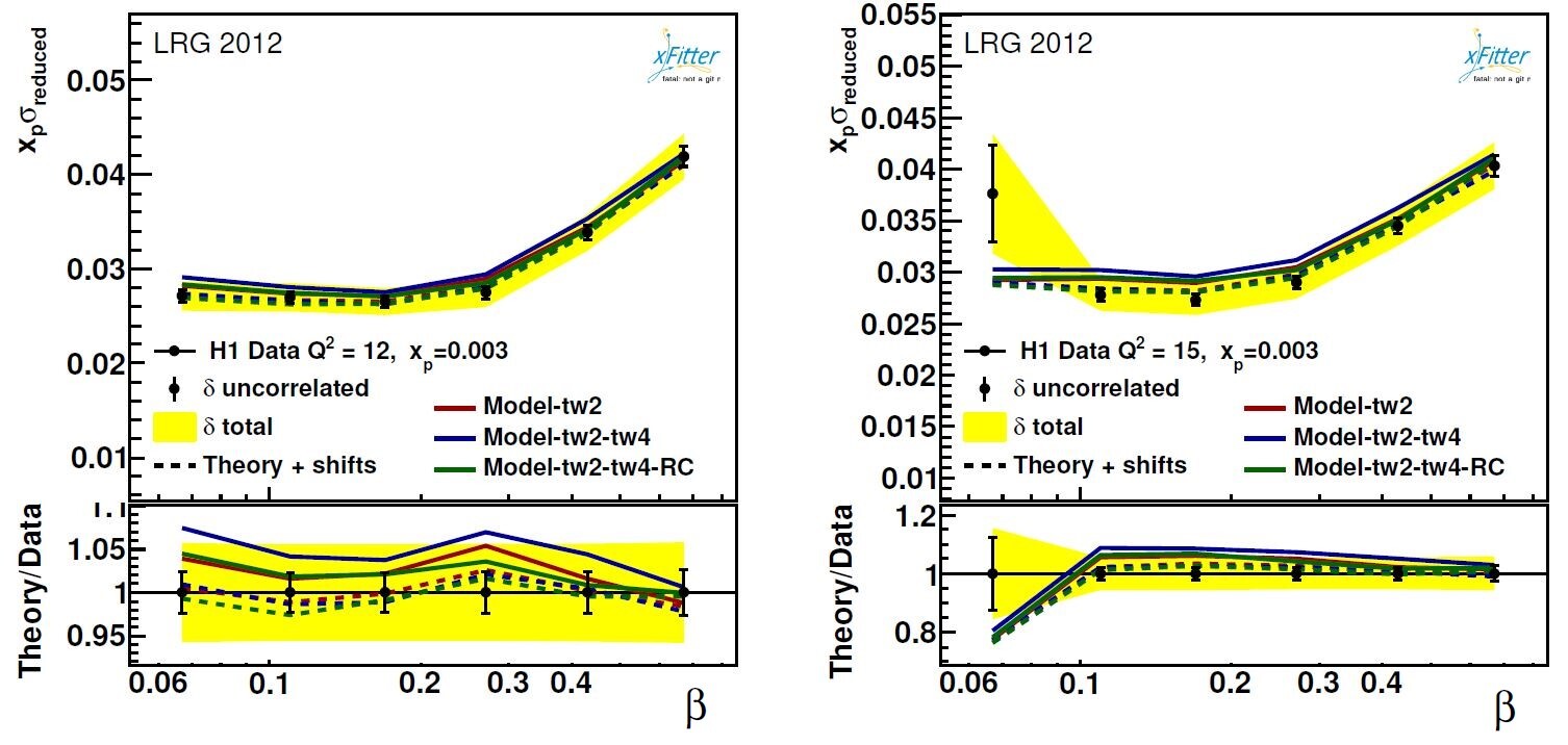
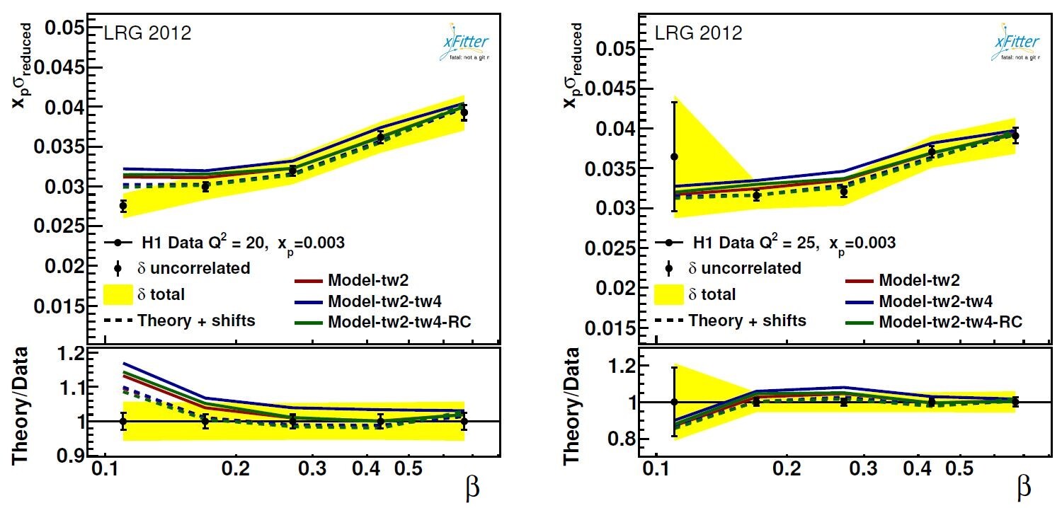
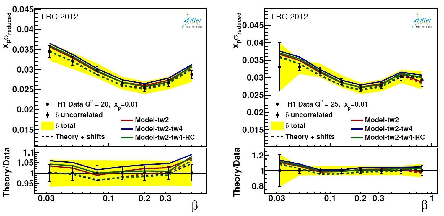
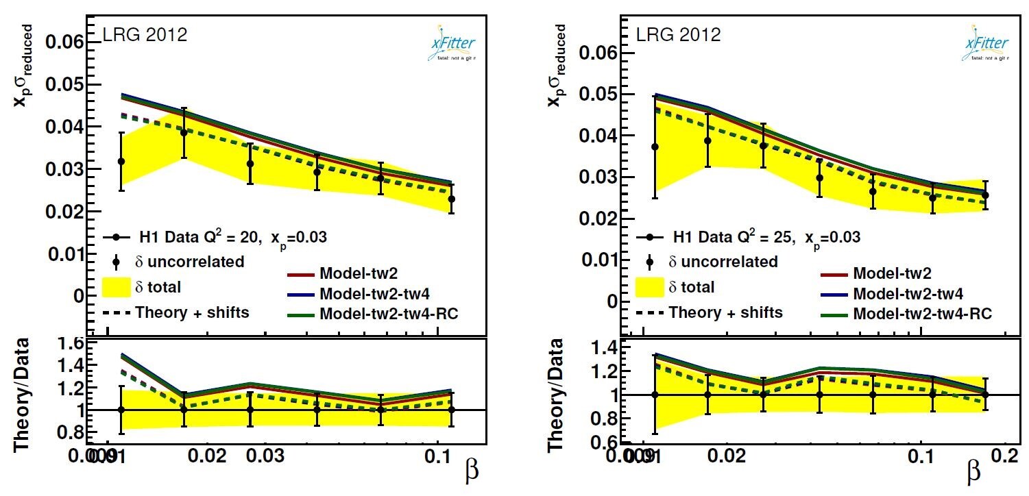
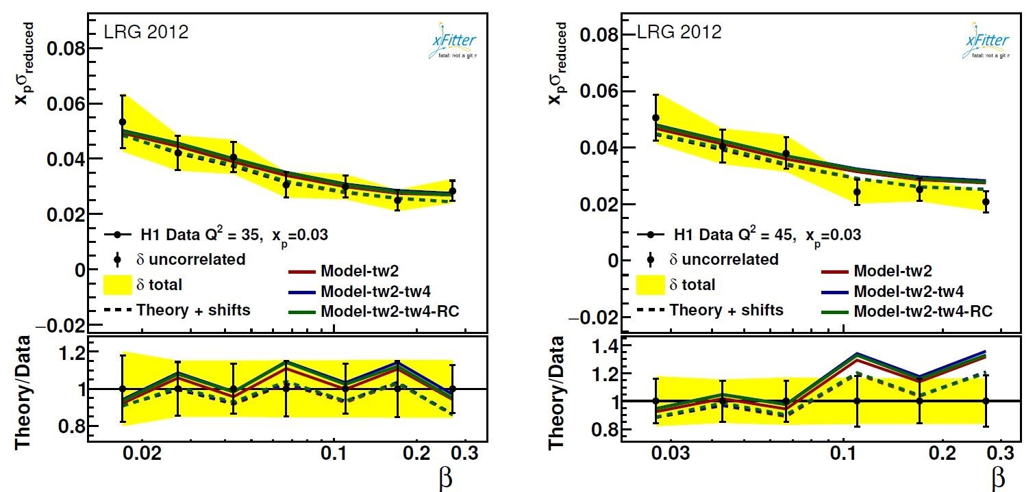
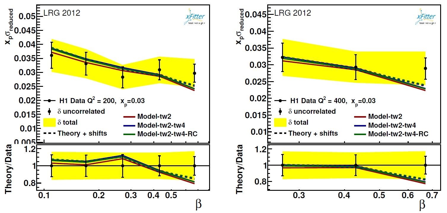
Figure 8: Same as Fig. 7 but this time for the H1-LRG-12 data.

Finally, in Fig. 9, we display a detailed comparison of the theory predictions using the three different sets of SKMHS22 and the H1/ZEUS combined data. The plots are presented as a function of $x_{I\!\!P}$ and for different values of $\beta$ and Q². As one can see, very good agreement is achieved.

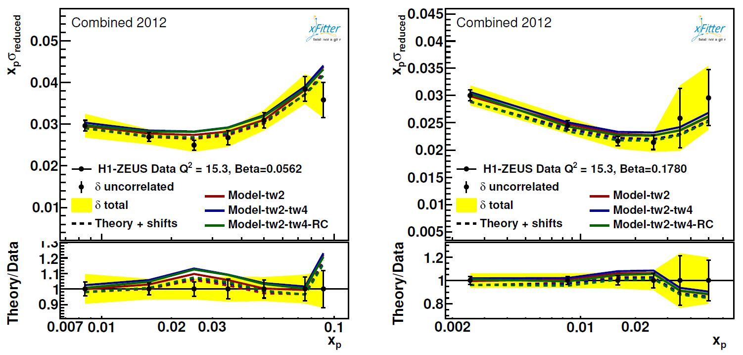
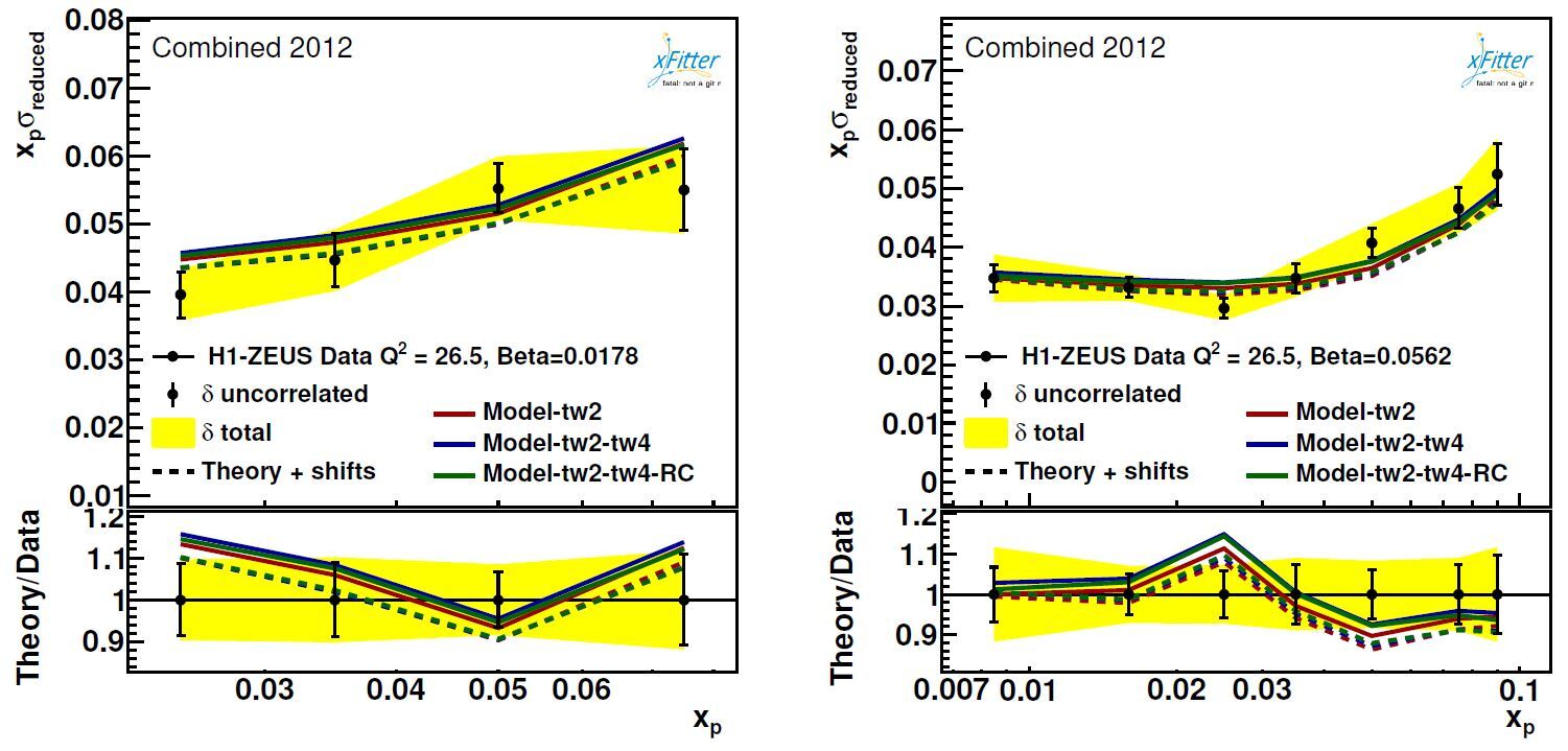
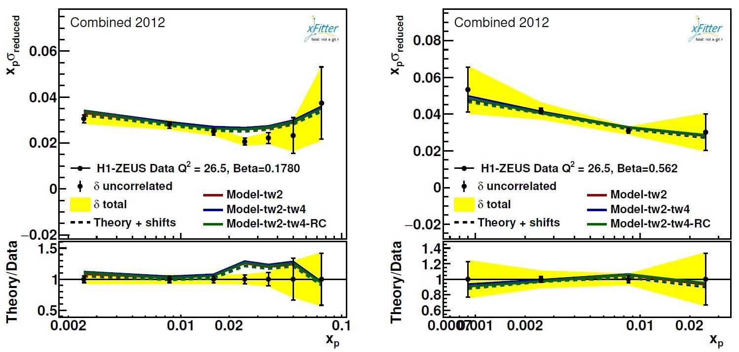
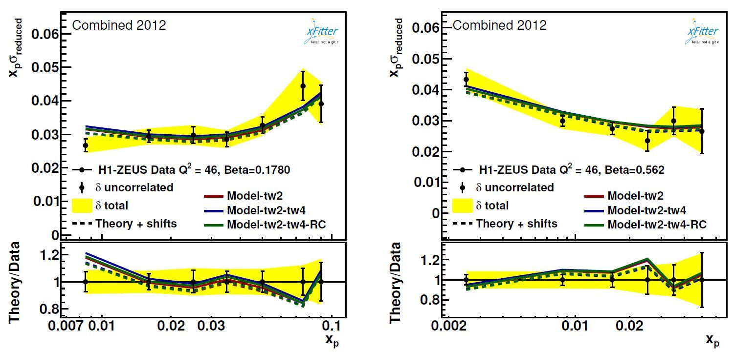
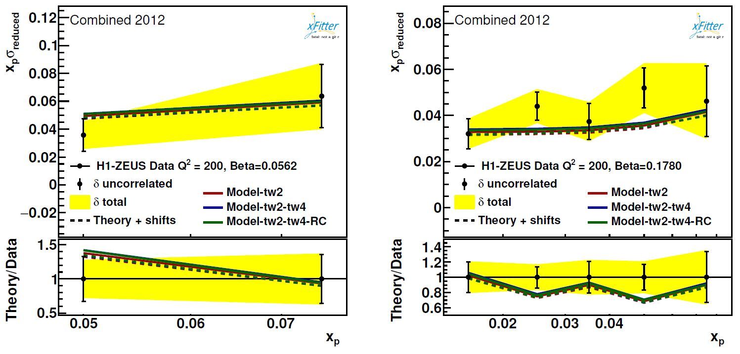
Figure 9: Same as Fig. 7 but this time for the H1/ZEUS combined data.

As one can see from Figs. 7, 8 and 9, in general, overall good agreement between the diffractive DIS data and the NLO theoretical predictions are achieved for all experiments, which is consistent with the individual and total $\chi^{2}$ values reported in Table. 3. Remarkably, the NLO theoretical predictions and the data are in reasonable agreement in the small- and large-$\beta$ regions, and the whole range of $x_{I\!\!P}$.

V Discussion and Conclusion

In this work, we performed fits of the diffractive PDFs at NLO accuracy in perturbative QCD called SKMHS22 using all available and up-to-date diffractive DIS data sets from the H1 and ZEUS Collaborations at HERA. We present a mutually consistent set of diffractive PDFs by adding the high-precision diffractive DIS data from the H1/ZEUS combined inclusive diffractive cross-sections measurements to the data sample.

In addition to the standard twist-2 contributions, we also considered the twist-4 correction and Reggeon contribution to the diffractive structure function, which dominate in the region of large $\beta$. The effect of such contributions on the diffractive PDFs and cross-sections were carefully examined and discussed. The twist-4 correction and Reggeon contribution lead to the gluon distribution which is peaked stronger at high-$\beta$ than in the case of the standard twist-2 QCD fit.

The well-established xFitter fitting methodology, widely used to determine the unpolarised PDFs, are modified to incorporate the higher-twist contributions. This fitting methodology is specifically designed to provide faithful representations of the experimental uncertainties on the PDFs.

The QCD analysis presented in this work represents the first step of a broader program. A number of updates and improvements are foreseen for the future study.

The important limitation of the SKMHS22 QCD analysis is the fact that it is based on the inclusive diffractive DIS cross-section measurements. Despite the fact that the diffractive DIS is the cleanest process for the extraction of diffractive PDF, it is scarcely sensitive to the gluon density. For the near future, our main aim is to include very recent diffractive dijet production data H1:2014pjf ; H1:2015okx , which we expect to provide a good constraint on the determination of the gluon diffractive PDFs. This will require the numerical implementation of the corresponding observables at NLO and NNLO accuracy in perturbative QCD in the xFitter package. A further improvement for the future SKMHS22 analyses, as a long-term project, is the inclusion of other observables from hadron colliders which could carry some information on flavor separation.

A FORTRAN subroutine, which evaluates the three sets of SKMHS22 NLO diffractive PDFs presented in this work for given values of $\beta$, $x_{I\!\!P}$ and Q² can be obtained from the authors upon request. These diffractive PDFs sets are available in the standard LHAPDF format.

- (1) S. Chekanov et al. [ZEUS], Deep inelastic scattering with leading protons or large rapidity gaps at HERA, Nucl. Phys. B 816, 1-61 (2009).
- (2) A. Aktas et al. [H1], Measurement and QCD analysis of the diffractive deep-inelastic scattering cross-section at HERA, Eur. Phys. J. C 48, 715-748 (2006).
- (3) S. Chekanov et al. [ZEUS], A QCD analysis of ZEUS diffractive data, Nucl. Phys. B 831, 1-25 (2010).
- (4) A. Aktas et al. [H1], Diffractive open charm production in deep-inelastic scattering and photoproduction at HERA, Eur. Phys. J. C 50, 1-20 (2007).
- (5) A. Aktas et al. [H1], Dijet Cross Sections and Parton Densities in Diffractive DIS at HERA, JHEP 10, 042 (2007).
- (6) Y. L. Dokshitzer, Calculation of the Structure Functions for Deep Inelastic Scattering and e+ e- Annihilation by Perturbation Theory in Quantum Chromodynamics, Sov. Phys. JETP 46, 641-653 (1977).
- (7) V. N. Gribov and L. N. Lipatov, Deep inelastic e p scattering in perturbation theory, Sov. J. Nucl. Phys. 15, 438-450 (1972)
- (8) L. N. Lipatov, The parton model and perturbation theory, Yad. Fiz. 20, 181-198 (1974)
- (9) G. Altarelli and G. Parisi, Asymptotic Freedom in Parton Language, Nucl. Phys. B 126, 298-318 (1977).
- (10) J. C. Collins, L. Frankfurt and M. Strikman, Diffractive hard scattering with a coherent pomeron, Phys. Lett. B 307, 161-168 (1993).
- (11) M. Wusthoff and A. D. Martin, The QCD description of diffractive processes, J. Phys. G 25, R309-R344 (1999).
- (12) A. Maktoubian, H. Mehraban, H. Khanpour and M. Goharipour, Role of higher twist effects in diffractive DIS and determination of diffractive parton distribution functions, Phys. Rev. D 100, no.5, 054020 (2019).
- (13) H. Khanpour, Phenomenology of diffractive DIS in the framework of fracture functions and determination of diffractive parton distribution functions, Phys. Rev. D 99, no.5, 054007 (2019).
- (14) M. Goharipour, H. Khanpour and V. Guzey, First global next-to-leading order determination of diffractive parton distribution functions and their uncertainties within the xFitter framework, Eur. Phys. J. C 78, no.4, 309 (2018).
- (15) F. A. Ceccopieri, Single-diffractive Drell–Yan pair production at the LHC, Eur. Phys. J. C 77, no.1, 56 (2017).
- (16) S. Alekhin, O. Behnke, P. Belov, S. Borroni, M. Botje, D. Britzger, S. Camarda, A. M. Cooper-Sarkar, K. Daum and C. Diaconu, et al. HERAFitter, Eur. Phys. J. C 75, no.7, 304 (2015).
- (17) H. Abdolmaleki et al. [xFitter Developers’ Team], “xFitter: An Open Source QCD Analysis Framework. A resource and reference document for the Snowmass study,” [arXiv:2206.12465 [hep-ph]].
- (18) L. Trentadue and G. Veneziano, Fracture functions: An Improved description of inclusive hard processes in QCD, Phys. Lett. B 323, 201-211 (1994).
- (19) D. de Florian and R. Sassot, QCD analysis of diffractive and leading proton DIS structure functions in the framework of fracture functions, Phys. Rev. D 58, 054003 (1998).
- (20) F. D. Aaron et al. [H1 and ZEUS], Combined inclusive diffractive cross sections measured with forward proton spectrometers in deep inelastic scattering at HERA, Eur. Phys. J. C 72, 2175 (2012).
- (21) G. Ingelman and P. E. Schlein, Jet Structure in High Mass Diffractive Scattering, Phys. Lett. B 152, 256-260 (1985).
- (22) J. C. Collins, L. Frankfurt and M. Strikman, Factorization for hard exclusive electroproduction of mesons in QCD, Phys. Rev. D 56, 2982-3006 (1997).
- (23) J. C. Collins, Factorization in hard diffraction, J. Phys. G 28, 1069-1078 (2002).
- (24) J. C. Collins, Proof of factorization for diffractive hard scattering, Phys. Rev. D 57, 3051-3056 (1998) [erratum: Phys. Rev. D 61, 019902 (2000)].
- (25) J. A. M. Vermaseren, A. Vogt and S. Moch, The Third-order QCD corrections to deep-inelastic scattering by photon exchange, Nucl. Phys. B 724, 3-182 (2005).
- (26) R. D. Ball, S. Carrazza, J. Cruz-Martinez, L. Del Debbio, S. Forte, T. Giani, S. Iranipour, Z. Kassabov, J. I. Latorre and E. R. Nocera, et al. The path to proton structure at 1% accuracy: NNPDF Collaboration, Eur. Phys. J. C 82, no.5, 428 (2022).
- (27) G. R. Boroun, Effect of the Parameterization of the Distribution Functions on the Longitudinal Structure Function at Small x, Pisma Zh. Eksp. Teor. Fiz. 114, no.1, 3 (2021).
- (28) L. A. Harland-Lang, A. D. Martin, P. Motylinski and R. S. Thorne, Parton distributions in the LHC era: MMHT 2014 PDFs, Eur. Phys. J. C 75, no.5, 204 (2015).
- (29) R. D. Ball, J. Butterworth, A. M. Cooper-Sarkar, A. Courtoy, T. Cridge, A. De Roeck, J. Feltesse, S. Forte, F. Giuli and C. Gwenlan, et al. The PDF4LHC21 combination of global PDF fits for the LHC Run III, [arXiv:2203.05506 [hep-ph]].
- (30) M. Salajegheh, S. M. Moosavi Nejad, M. Soleymaninia, H. Khanpour and S. Atashbar Tehrani, NNLO charmed-meson fragmentation functions and their uncertainties in the presence of meson mass corrections, Eur. Phys. J. C 79, no.12, 999 (2019).
- (31) M. Salajegheh, S. M. Moosavi Nejad, H. Khanpour, B. A. Kniehl and M. Soleymaninia, -hadron fragmentation functions at next-to-next-to-leading order from a global analysis of annihilation data, Phys. Rev. D 99, no.11, 114001 (2019).
- (32) M. Soleymaninia, H. Hashamipour, H. Khanpour and H. Spiesberger, Fragmentation Functions for Using Neural Networks, [arXiv:2202.05586 [hep-ph]].
- (33) R. S. Thorne, Effect of changes of variable flavor number scheme on parton distribution functions and predicted cross sections, Phys. Rev. D 86, 074017 (2012).
- (34) M. Buza, Y. Matiounine, J. Smith and W. L. van Neerven, Charm electroproduction viewed in the variable flavor number scheme versus fixed order perturbation theory, Eur. Phys. J. C 1, 301-320 (1998).
- (35) L. A. Harland-Lang, A. D. Martin, P. Motylinski and R. S. Thorne, Charm and beauty quark masses in the MMHT2014 global PDF analysis, Eur. Phys. J. C 76, no.1, 10 (2016).
- (36) M. Tanabashi et al. [Particle Data Group], Review of Particle Physics, Phys. Rev. D 98, no.3, 030001 (2018).
- (37) K. Golec-Biernat and A. Luszczak, Dipole model analysis of the newest diffractive deep inelastic scattering data, Phys. Rev. D 79, 114010 (2009).
- (38) K. J. Golec-Biernat and A. Luszczak, Diffractive parton distributions from the analysis with higher twist, Phys. Rev. D 76, 114014 (2007).
- (39) K. J. Golec-Biernat and M. Wusthoff, Saturation effects in deep inelastic scattering at low Q**2 and its implications on diffraction, Phys. Rev. D 59, 014017 (1998).
- (40) K. J. Golec-Biernat and J. Kwiecinski, Subleading Reggeons in deep inelastic diffractive scattering at HERA, Phys. Rev. D 55, 3209-3211 (1997).
- (41) K. J. Golec-Biernat, J. Kwiecinski and A. Szczurek, Reggeon and pion contributions in semiexclusive diffractive processes at HERA, Phys. Rev. D 56, 3955-3960 (1997).
- (42) A. Aktas et al. [H1], Diffractive deep-inelastic scattering with a leading proton at HERA, Eur. Phys. J. C 48, 749-766 (2006).
- (43) F. D. Aaron et al. [H1], Measurement of the Diffractive Longitudinal Structure Function at HERA, Eur. Phys. J. C 71, 1836 (2011).
- (44) F. D. Aaron et al. [H1], Inclusive Measurement of Diffractive Deep-Inelastic Scattering at HERA, Eur. Phys. J. C 72, 2074 (2012).
- (45) F. D. Aaron, C. Alexa, V. Andreev, S. Backovic, A. Baghdasaryan, E. Barrelet, W. Bartel, K. Begzsuren, A. Belousov and J. C. Bizot, et al. Measurement of the cross section for diffractive deep-inelastic scattering with a leading proton at HERA, Eur. Phys. J. C 71, 1578 (2011).
- (46) S. Chekanov et al. [ZEUS], Dissociation of virtual photons in events with a leading proton at HERA, Eur. Phys. J. C 38, 43-67 (2004).
- (47) F. D. Aaron et al. [H1], Inclusive Deep Inelastic Scattering at High with Longitudinally Polarised Lepton Beams at HERA, JHEP 09, 061 (2012).
- (48) F. James and M. Roos, Minuit: A System for Function Minimization and Analysis of the Parameter Errors and Correlations, Comput. Phys. Commun. 10, 343-367 (1975).
- (49) P. M. Nadolsky, H. L. Lai, Q. H. Cao, J. Huston, J. Pumplin, D. Stump, W. K. Tung and C. P. Yuan, Implications of CTEQ global analysis for collider observables, Phys. Rev. D 78, 013004 (2008).
- (50) V. Andreev et al. [H1], Diffractive Dijet Production with a Leading Proton in Collisions at HERA, JHEP 05, 056 (2015).
- (51) V. Andreev et al. [H1], Measurement of Dijet Production in Diffractive Deep-Inelastic ep Scattering at HERA, JHEP 03, 092 (2015).