DistSPECTRL: Distributing Specifications in Multi-Agent Reinforcement Learning Systems

Abstract

While notable progress has been made in specifying and learning objectives for general cyber-physical systems, applying these methods to distributed multi-agent systems still pose significant challenges. Among these are the need to (a) craft specification primitives that allow expression and interplay of both local and global objectives, (b) tame explosion in the state and action spaces to enable effective learning, and (c) minimize coordination frequency and the set of engaged participants for global objectives. To address these challenges, we propose a novel specification framework that allows natural composition of local and global objectives used to guide training of a multi-agent system. Our technique enables learning expressive policies that allow agents to operate in a coordination-free manner for local objectives, while using a decentralized communication protocol for enforcing global ones. Experimental results support our claim that sophisticated multi-agent distributed planning problems can be effectively realized using specification-guided learning. Code is provided at https://github.com/yokian/distspectrl.

1 Introduction

Reinforcement Learning (RL) can be used to learn complex behaviors in many different problem settings. A main component of RL is providing feedback to an agent via a reward signal. This signal should encourage desired behaviors, and penalize undesirable ones, enabling the agent to eventually proceed through a sequence of tasks and is designed by the programmer beforehand. A commonly used technique to encode tasks in a reward signal is the sparse method of providing zero reward until a task is completed upon which a non-zero reward is given to the agent. Because this procedure has the significant shortcoming of delaying generating a useful feedback signal for a large portion of the agent-environment interaction process, a number of alternative techniques have been proposed [14, 1].

Formulating a reward signal that reduces the sparsity of this feedback is known as reward shaping. Often, this is done manually but a more general, robust method would be to automatically shape a reward given a specification of desired behavior. Spectrl [5] proposes a reward shaping mechanism for a set of temporal logic specifications on a single-agent task that uses a compiled a finite-state automaton called a task monitor. Reward machines [19, 2, 18] are another objective-specifying method for RL problems that also define a finite automaton akin to the ones used in Spectrl, with some subtle differences such as the lack of registers (used by the task monitor for memory).

Distributed multi-agent applications however, introduce new challenges in automating this reward shaping process. Agents have their own respective goals to fulfill as well as coordinated goals that must be performed in cooperation with other agents. While the expressiveness of the language in Spectrl lends itself, with minor extensions, to specifying these kinds of goals, we require new compilation and execution algorithms to tackle inherent difficulties in multi-agent reinforcement learning (MARL); these include credit assignment of global objectives and the presence of large state and action spaces that grow as the number of agents increases. Learning algorithms for multi-agent problems have often encouraged distribution as a means of scaling in the presence of state and action space explosion. This is because purely centralized approaches have the disadvantages of not only requiring global knowledge of the system at all times but also induce frequent and costly synchronized agent control.

To address these issues, we develop a new specification-guided distributed multi-agent reinforcement learning framework. Our approach has four main features. First, we introduce two classes of predicates (viz. local and global) to capture tasks in a multi-agent world (Sec. 4). Second, we develop a new procedure for generating composite task monitors using these predicates and devise new techniques to distribute these monitors over all agents to address scalability and decentralization concerns (Sec. 5). Third, we efficiently solve the introduced problem of subtask synchronization (Sec. 6) among agents via synchronization states in the task monitors. Lastly, we describe a wide class of specification structures (Sec. 7) amenable to scaling in the number of agents and provide a means to perform such a scaling (Sec. 8).

By using these components in tandem, we provide the first solution to composing specifications and distributing them among agents in a scalable fashion within a multi-agent learning scenario supporting continuous state and action spaces. Before presenting details of our approach, we first provide necessary background information (Sec. 2) and formalize the problem (Sec. 3).

2 Background

Markov Decision Processes

Reinforcement learning is a tool to solve Markov Decision Processes (MDPs). MDPs are tuples of the form $\langle\mathcal{S},D,A,P,R,T\rangle$ where $\mathcal{S}\in\mathbb{R}^{n}$ is the state space, $D$ is the initial state distribution, $A\in\mathbb{R}^{m}$ is the action space, $P:\mathcal{S}\times A\times\mathcal{S}\rightarrow[0,1]$ is the transition function, and $T$ is the time horizon. A rollout $\zeta\in Z$ of length $T$ is a sequence of states and actions $\zeta=(s_{0},a_{0},...,a_{T-1},s_{T})$ where $s_{i}\in\mathcal{S}$ and $a_{i}\in A$ are such that $s_{i+1}\sim P(s_{i},a_{i})$. $R:Z\rightarrow\mathbb{R}$ is a reward function used to score a rollout $\zeta$.

Multi-Agent Reinforcement Learning

A Markov game with $\mathcal{N}=\{1,\cdots,N\}$ denoting the set of $N$ agents is a tuple $\mathcal{M}_{g}=\langle\mathcal{N},\{\mathcal{S}^{i}\}_{i\in\mathcal{N}},D,\{A^{i}\}_{i\in\mathcal{N}},P,\{R^{i}\}_{i\in\mathcal{N}},T\rangle$ where ${A^{i}}$, ${R^{i}}$ define their agent-specific action spaces and reward functions. They are a direct generalization of MDPs to the multi-agent scenario. Let $\mathcal{S}_{m}=\{\mathcal{S}^{i}\}_{i\in\mathcal{N}}$ and $A_{m}=\{A^{i}\}_{i\in\mathcal{N}}$, then $P:\mathcal{S}_{m}\times A_{m}\times\mathcal{S}_{m}\rightarrow[0,1]$ is the transition function. A rollout $\zeta_{m}\in Z_{m}$ here corresponds to $\zeta_{m}=(\bar{s}_{0},\bar{a}_{0},...,\bar{a}_{T-1},\bar{s}_{T})$ where $\bar{s}\in\mathcal{S}_{m}$ and $\bar{a}\in A_{m}$. We also define an agent specific rollout $\zeta^{i}_{m}\in Z^{i}_{m},~{}\zeta^{i}_{m}=(s^{i}_{0},a^{i}_{0},...,a^{i}_{T-1},s^{i}_{T})$ where $s^{i}\in\mathcal{S}^{i}$ and $a^{i}\in A^{i}$. $D$ is the initial state distribution over $\mathcal{S}_{m}$.

Agents attempt to learn a policy $\pi^{i}:\mathcal{S}^{i}\rightarrow\Delta(A^{i})$ such that $\mathbb{E}\left[\sum_{t}R^{i}_{t}|\pi^{i},\pi^{-i}\right]$ is maximized, where $\Delta(A^{i})$ is a probability distribution over $A^{i}$ and $\pi^{-i}$ is the set of all policies apart from $\pi^{i}$. We use $\Pi=\{\pi^{i}\}_{i\in\mathcal{N}}$ to denote the set of all agent policies. For simplicity, we restrict our formulation to a homogeneous set of agents which operate over the same state ($\mathcal{S}^{i}=\mathcal{S}_{A}$) and action space ($A^{i}=A_{A}$).

SPECTRL

Jothimurugan et. al [5] introduce a specification language for reinforcement learning problems built using temporal logic constraints and predicates. It is shown to be adept at handling complex compositions of task specifications through the use of a task monitor and well-defined monitor transition rules. Notably, one can encode Non-Markovian tasks into the MDP using the additional states of the automaton (task monitor) compiled from the given specification.

The atomic elements of this language are Boolean predicates $b$ defined as functions of a state $\mathcal{S}$ with output $\llbracket b\rrbracket:\mathcal{S}\rightarrow\mathbb{B}$. These elements have quantitative semantics $\llbracket b\rrbracket_{q}$ with the relation being $\llbracket b\rrbracket(s)=\mathtt{True}\iff\llbracket b\rrbracket_{q}(s)>0$. Specifications $\phi$ are Boolean functions of the state trajectory $\zeta=(s_{1},s_{2},...,s_{T})$. The specification language also includes composition functions for a specification $\phi$ and Boolean predicate $b$, with the language defined as

$$\phi::=\mathtt{achieve}~{}b~{}|~{}\phi~{}\mathtt{ensuring}~{}b~{}|~{}\phi_{1};~{}\phi_{2}~{}|~{}\phi_{1}~{}\mathtt{or}~{}\phi_{2}$$

The description of these functions is as follows. $\mathtt{achieve}~{}b$ is true when the trajectory satisfies $b$ at least once. $\phi~{}\mathtt{ensuring}~{}b$ is true when $b$ is satisfied at all timesteps in the trajectory. $\phi_{1};~{}\phi_{2}$ is a sequential operator that is true when, in a given trajectory $\zeta=(s_{1},s_{2},...,s_{T})$, $\exists~{}k>1$ such that $\phi_{1}(s_{1},...,s_{k})$ is true and $\phi_{2}(s_{k+1},...,s_{T})$ is true. In other words, $\phi_{1};~{}\phi_{2}$ represents an ordered sequential completion of specification $\phi_{1}$ followed by $\phi_{2}$. Lastly, $\phi_{1}~{}\mathtt{or}~{}\phi_{2}$ is true when a trajectory satisfies either $\phi_{1}$ or $\phi_{2}$.

Given a specification $\phi$ on a Markov Decision Process $\langle S,D,A,P,T\rangle$ (MDP) defined using Spectrl, a task monitor $\langle Q,X,\Sigma,U,\Delta,q_{0},v_{0},F,\rho\rangle$ (a finite state automaton [20]) is compiled to record the completion status of tasks with monitor states $Q$; final monitor states $F$ denote a satisfied trajectory. This is used to create an augmented version of the MDP $\langle\tilde{S},\tilde{s_{0}},\tilde{A},\tilde{P},\tilde{R},\tilde{T}\rangle$ with an expanded state, action space and modified reward function . The task monitor provides a scoring function for trajectories in the augmented MDP to guide policy behavior.

While Spectrl has been shown to work with trajectory-based algorithms for reinforcement learning [12], it is not immediately evident how to translate it to common RL algorithms such as DDPG [10] and PPO [16]. A simple solution would be to keep the episodic format with a trajectory $\zeta=(s_{0},\cdots,s_{T})$ and assign the trajectory value of Spectrl (a function of $\zeta$) to the final state transition in the trajectory $s_{T-1}\rightarrow s_{T}$ and zero for all other states. Importantly, this maintains the trajectory ordering properties of Spectrl in the episodic return $(\sum_{t=0}^{T}r_{t})$.

3 Problem Statement

Directly appropriating Spectrl for our use case of imposing specifications on multi-agent problems poses significant scalability issues. Consider the case

$$\phi_{a}=\mathtt{achieve}(\mathtt{reach}(P));\mathtt{achieve}(\mathtt{reach}(Q))$$

where $\llbracket\mathtt{reach}(P)\rrbracket=\mathtt{True}$ when an agent reaches state $P$. To ease the illustration of our framework, we assume that all agents are homogeneous, i.e. $\mathcal{S}^{i}=\mathcal{S}_{A},\forall i\in\mathcal{N}$. Now, the state space of the entire multi-agent system is $\mathcal{S}=(\mathcal{S}_{A})^{N}$ for $N$ agents (we omit $m$ for perspicuity).

If the predicate $\mathtt{reach}$ was defined on the entire state $\mathcal{S}$, it would yield a specification forcing synchronization between agents. On the other hand, if $\mathtt{reach}$ was defined on the agent state $\mathcal{S}_{A}$, then it would create a localized specification where synchronization is not required. This would be akin to allowing individual agents to act independently of other agent behaviors.

However, using a centralized task monitor for the localized predicate would cause the number of monitor states to exponentially increase with the number of agents $N$ and subtasks $K$ since the possible stages of task completion would be $\mathcal{O}(K^{N})$.

To address this scalability issue, the benefits of task monitor distribution are apparent. In the case of $\phi_{a}$ above, assume $\mathtt{reach}$ is defined on the local state space $\mathcal{S}_{A}$. If each agent had a separate task monitor stored locally to keep track of the task completion stages, the new number of monitor states is now reduced to $\mathcal{O}(NK)$.

Consider an example of robots in a warehouse. A few times a day, all robots must gather at a common point for damage inspection at the same time (akin to a global reach) to minimize the frequency of inspection (an associated cost). To ensure satisfaction of the entire specification, the reward given to an RL agent learning this objective should capture both the global and local tasks. For example, if the global reach task for the routine inspection is made local instead, the cost incurred may be larger than if it was a synchronized global objective.

Main Objective

Given a specification $\phi$ on a system of $N$ agents, we wish to find policies $\Pi=\{\pi^{1},\cdots,\pi^{N}\}$ to maximize the probability of satisfying $\phi$ for all agents. Formally, we seek

$$\Pi^{*}\in\underset{\pi^{1},\cdots,\pi^{N}}{\arg\max}~{}~{}\underset{\zeta_{m}\sim D_{\Pi}}{\text{Pr}}\left[\llbracket\phi(\zeta_{m})\rrbracket=\mathtt{True}\right]$$

where $D_{\Pi}$ is the distribution of all system rollouts when all agents collectively follow policy set $\Pi$. We emphasize that $\phi$ acts on the entire rollout, $\phi:Z_{m}\rightarrow\{0,1\}$ and not in an agent-specific manner, $\phi^{\prime}:Z^{i}_{m}\rightarrow\{0,1\}$. This discourages agents from attempting to simply satisfy their local objectives while preventing the system from achieving necessary global ones.

Figure 1: Example Composite Task Monitor for specification $\phi_{ex}$ (Sec. 4) with 4 task goals denoted by Q,P,P’ and R where the agent starts at $q_{0}$. Double circles represent final states while green circles represent global states. The diagram removes a state between $q_{1}$ and $(q_{3},q_{4})$ as well as self-loops for ease of explanation.

4 SPECTRL in a Multi-Agent World

Unlike the single agent case, multi-agent problems have two major classes of objectives. Agents have individual goals to fulfill as well as collective goals that require coordination and/or global system knowledge. These individual goals are often only dependent on the agent-specific state $s^{i}$ while collective goals require full system knowledge $\bar{s}$.

Consequently, for a multi-agent problem, we see the need for two types of predicates viz. local and global. Local predicates are of the form $p_{lo}:\mathcal{S}_{A}\rightarrow\mathbb{B}$ whereas global predicates have the form $p_{gl}:\mathcal{S}\rightarrow\mathbb{B}$ where $\mathbb{B}$ is the Boolean space. We introduce two simple extensions of $\mathtt{reach}$ [5] to demonstrate the capabilities of this distinction.

Local predicates are defined with respect to each agent and represent our individual goals. As an example, closely related to the problems observed in Spectrl, we introduce the following local predicates for a state $s_{a}\in\mathcal{S}_{A}$,

$$\llbracket\mathtt{reach}_{lo}x\rrbracket(s_{a})=(||s_{a}-x||_{\infty}<1)$$

which represents reaching near location $x$ in terms of the $L_{\infty}$ norm. Now to enforce global restrictions, we introduce counterparts to these predicates that act on a global state $\bar{s}\in\mathcal{S}$.

$$\llbracket\mathtt{reach}_{gl}\bar{x}\rrbracket(\bar{s})=(||\bar{s}-\bar{x}||_{\infty}<1)$$

where we now have a set of locations $\bar{x}\in\mathcal{S}$.

As in Spectrl, each of these predicates $b$ require quantitative semantics $\llbracket b\rrbracket_{q}$ to facilitate our reward shaping procedure. We define these semantics as follows:

• $\mathtt{reach}_{lo}$ has the same semantics as $\mathtt{reach}$ in [5] yet is defined on space $\mathcal{S}_{A}$.

  $$\llbracket\mathtt{reach}_{lo}x\rrbracket_{q}(s_{a})=1-d_{\infty}(s_{a},x)$$

  where $d_{\infty}(a,b)$ represents the $L_{\infty}$ distance between $a$ and $b$ with the usual extension to the case where $b$ is a set.

• $\mathtt{reach}_{gl}$ is defined on the state space $\mathcal{S}$ as

  $$\llbracket\mathtt{reach}_{gl}\bar{x}\rrbracket_{q}(\bar{s})=1-d_{\infty}(\bar{s},\bar{x})$$

We observe that the same composition rules can apply to these predicates and we thus attempt to solve RL systems described with these compositions. As shown in Sec. 3, using a centralized Spectrl compilation algorithm on the entire state space, even for simple sequences of tasks, leads to an explosion in monitor states. We, therefore, distribute task monitors over agents to handle scalability. Furthermore, we also need to change Spectrl’s compilation rules to handle mixed objective compositions such as

$$\phi=\mathtt{reach}_{lo}(P);\mathtt{reach}_{gl}(Q);\mathtt{reach}_{gl}(R)$$

To compile these specifications into a usable format, we utilize a composite task monitor as described in Sec. 5 and develop a new algorithm to achieve our goal. As an example, see Fig. 1 depicting a task monitor whose specification is:

$$\phi_{ex}= \mathtt{reach}_{gl}(P^{\prime})\ \mathtt{or}\ \mathtt{reach}_{lo}(Q);\left[\mathtt{reach}_{lo}(P)\ \mathtt{or}\ \mathtt{reach}_{gl}(R)\right]$$

Here, we have 4 task goals denoted by $P,Q,R$ and $P^{\prime}$. The agents all start at the root node $q_{0}$. States $q_{2}$, $q_{3}$ and $q_{4}$ are all final states in the task monitor while $q_{2}$ and $q_{4}$ are global monitor states. As shown in Sec. 6, $q_{0}$ and $q_{1}$ are a synchronization states. While it may seem that agents only require coordination at global states, it is also necessary for the agents to have the same task transition at these synchronization states as well.

5 Compilation Steps

Given a specification $\phi$ and the Markov game $\mathcal{M}_{g}$, we create a task monitor $M$ that is distributed among agents by making agent-specific copies. This is used to create an augmented Markov game $\mathcal{M}^{\prime}_{g}=\langle\mathcal{N},\{\tilde{\mathcal{S}}_{A}\}_{i\in\mathcal{N}},\tilde{D},\{\tilde{A}_{A}\}_{i\in\mathcal{N}},\tilde{P},\{\tilde{R}^{i}\}_{i\in\mathcal{N}},T\rangle$ on which the individual agent policies are trained.

Create Composite Task Monitor

When the types of specifications are divided into two based on the domain, the solution can be modeled with a composite task monitor $M_{\phi}=\langle Q,\tilde{X},\tilde{\Sigma},\tilde{U},\tilde{\Delta},q_{0},v_{0},F,\rho\rangle$. As in Spectrl, $Q$ is a finite set of monitor states. $\tilde{X}=X_{l}\cup X_{g}$ is a finite set of registers that are partitioned into $X_{l}$ for local predicates and $X_{g}$ for global predicates. These registers are used to keep track of the degree of completion of the task at the current monitor state for local and global tasks respectively.

We describe below how to use the compiled composite task monitor to create an augmented Markov game $\mathcal{M}_{g}^{\prime}$. Each $\tilde{\mathcal{S}}_{A}$ in $\mathcal{M}_{g}^{\prime}$ is an augmented state space with an augmented state being a tuple $(s_{A},q,v)\in\mathcal{S}_{A}\times Q\times V$ where $V\in\mathbb{R}^{X}$ and $v\in V$ is a vector describing the register values.

$\tilde{\Delta}=\Delta_{l}\cup\Delta_{g}$ houses the transitions of our task monitor. We require that: i) different transitions are allowed only under certain conditions defined by our states and register values; and, ii) furthermore, they must also provide rules on how to update the register values during each transition. To define these conditions for transition availability, we use $\tilde{\Sigma}=\Sigma_{l}\cup\Sigma_{g}$ where $\Sigma_{l}$ is a set of predicates over $\mathcal{S}_{A}\times V$ and $\Sigma_{g}$ is a set of predicates over $\mathcal{S}\times V$. Similarly, $\tilde{U}=U_{l}\cup U_{g}$ where $U_{l}$ is a set of functions $u_{l}:\mathcal{S}_{A}\times V\rightarrow V$ and $U_{g}$ is a set of functions $u_{g}:\mathcal{S}\times V\rightarrow V$. Now, we can define $\tilde{\Delta}\subseteq Q\times\tilde{\Sigma}\times\tilde{U}\times Q$ to be a finite set of transitions that are non-deterministic. Transition $(q,\sigma,u,q^{\prime})\in\tilde{\Delta}$ is an augmented transition either representing $(s^{i},q,v)\xrightarrow{a^{i}|\Pi_{-i}}((s^{i})^{\prime},q^{\prime},u_{l}(s^{i},v))$ or the form $(\bar{s},q,v)\xrightarrow{a^{i}|\Pi_{-i}}(\bar{s}^{\prime},q^{\prime},u_{g}(s,v))$ depending on whether $\sigma\in\Sigma_{l}$ or $\sigma\in\Sigma_{g}$ respectively. Let $\delta_{l}\in\Delta_{l}$ represent the former (localized) and $\delta_{g}\in\Delta_{g}$ the latter (global) transition types. Here $\Pi_{-i}$ denotes the policy set of all agents except agent $i$. Lastly, $q_{0}$ is the initial monitor state and $v_{0}$ is the initial register value (for all agents), $F\subseteq Q$ is the set of final monitor states, and $\rho:\mathcal{S}\times F\times V\rightarrow\mathbb{R}$ is the reward function.

Copies of these composite task monitors $M$ are distributed over agents $\mathcal{N}$ to form the set $\{M^{i}\}_{i\in\mathcal{N}}$. These individually stored task monitors are used to let each agent $i\in\mathcal{N}$ keep track of its subtasks and the degree of completion of those subtasks by means of monitor state $q^{i}$ and register value $v^{i}$.

Create Augmented Markov Game

From our specification $\phi$ we create the augmented Markov game $\mathcal{M}_{g}^{\prime}=\langle\mathcal{N},\{\tilde{\mathcal{S}}_{A}\}_{i\in\mathcal{N}},\tilde{D},\{\tilde{A}_{A}\}_{i\in\mathcal{N}},\tilde{P},\{\tilde{R}^{i}\}_{i\in\mathcal{N}},T\rangle$ using the compiled composite task monitor $M$ . A set of policies $\tilde{\Pi}^{*}$ that maximizes rewards in $\mathcal{M}_{g}^{\prime}$ should maximize the chance of the specification $\phi$ being satisfied.

Each $\tilde{\mathcal{S}}_{A}=\mathcal{S}_{A}\times Q\times V$ and $\tilde{D}=(\{s_{0}\}_{i\in\mathcal{N}},q_{0},v_{0})$. We use $\Delta$ to augment the transitions of $P$ with monitor transition information. Since $\Delta$ may contain non-deterministic transitions, we require the policies $\tilde{\Pi}$ to decide which transition to choose. Thus $\tilde{A}_{A}=A_{A}\times A_{\phi}$ where $A_{\phi}=\Delta$ chooses among the set of available transitions at a monitor state $q$. Since monitors are distributed among all agents in $\mathcal{N}$, we denote the set of current monitor states as $\bar{q}=\{q^{i}\}_{i\in\mathcal{N}}$ and the set of register values as $\bar{v}=\{v^{i}\}_{i\in\mathcal{N}}$. Now, each agent policy must output an augmented action $(a,\delta)\in\tilde{A}_{A}$ with the condition that $\delta_{l}=(q,\sigma_{l},u_{l},q^{\prime})$ is possible in local augmented state $\tilde{s}_{a}=(s_{a},q,v)$ if $\sigma_{l}(s_{a},v)$ is $\mathtt{True}$ and $\delta_{g}=(q,\sigma_{g},u_{g},q^{\prime})$ is possible in global augmented state $\tilde{s}=(\bar{s},\bar{q},\bar{v})$ if $\sigma_{g}(\bar{s},v)$ is $\mathtt{True}$. We can write the augmented transition probability $\tilde{P}$ as,

$$\tilde{P}((\bar{s},q,v),(a,(q,\sigma,u,q^{\prime})),(\bar{s}^{\prime},q^{\prime},u(\bar{s},v))))=P(\bar{s},a,\bar{s}^{\prime})$$

for transitions $\delta_{g}\in\Delta_{g}$ with $(\sigma,u)=(\sigma_{g},u_{g})$ and transitions $\delta_{l}\in\Delta_{l}$ with $(\sigma,u)=(\sigma_{l},u_{l})$. Here, we let $u_{l}(\bar{s},v)=u_{l}(s^{i},v)$ for agent $i$ since $s^{i}$ is included in $\bar{s}$. An augmented rollout $\tilde{\zeta}_{m}$ where

$$\tilde{\zeta}_{m}=((\bar{s}_{0},\bar{q}_{0},\bar{v}_{0}),\bar{a}_{0},...,\bar{a}_{T-1},(\bar{s}_{T},\bar{q}_{T},\bar{v}_{T}))$$

is formed by these augmented transitions. To translate this trajectory back into the Markov game $\mathcal{M}_{g}$ we can perform projection $\mathtt{proj}(\tilde{\zeta}_{m})=(\bar{s}_{0},\bar{a}_{0},...,\bar{a}_{T-1},\bar{s}_{T},)$.

Determine Shaped Rewards

Now that we have the augmented Markov game $\mathcal{M}_{g}^{\prime}$ and compiled our composite task monitor, we proceed to form our reward function that encourages the set of policies $\Pi$ to satisfy our specification $\phi$. We can perform shaping in a manner similar to Spectrl’s single-agent case on our distributed task monitor. Crucially, since reward shaping is done during the centralized training phase, we can assume we have access to the entire augmented rollout namely $\tilde{s}_{t}=(\bar{s}_{t},\bar{q}_{t},\bar{v}_{t})$ at any given $t\in[0,T]$. From the monitor reward function $\rho$, we can determine the weighting for a complete augmented rollout as

$$\tilde{R}^{i}(\tilde{\zeta}_{m})=\begin{cases}\rho(\bar{s}_{T},q^{i}_{T},v^{i}_{T}),&\text{if}\ q^{i}_{T}\in F\\ -\infty&\text{otherwise}\end{cases}$$

Theorem 5.1

(Proof in Appendix Sec. 0.F.) For any Markov game $\mathcal{M}_{g}$, specification $\phi$ and rollout $\zeta_{m}$ of $\mathcal{M}_{g}$, $\zeta_{m}$ satisfies $\phi$ if and only if there exists an augmented rollout $\tilde{\zeta}_{m}$ such that i) $\tilde{R}^{i}(\tilde{\zeta}_{m})>0~{}\forall~{}i\in\mathcal{N}$ and ii) $\mathtt{proj}(\tilde{\zeta}_{m})=\zeta_{m}$.

The $\tilde{R}^{i}$ specified is $-\infty$ unless a trajectory reached a final state of the composite task monitor. To reduce the sparsity of this reward signal, we transform this into a shaped reward $\tilde{R}_{s}^{i}$ that gives partial credit to completing subtasks in the composite task monitor.

Define for a non-final monitor state $q\in Q\setminus F$, function $\alpha:\mathcal{S}\times Q\times V\rightarrow\mathbb{R}$.

$$\alpha(\bar{s},q,v)=\underset{(q,\sigma,u,q^{\prime})\in\Delta,q\neq q^{\prime}}{\max}\llbracket\sigma\rrbracket_{q}(\bar{s},v)$$

This represents how close an augmented state $\tilde{s}=(\bar{s},q,v)$ is to transition to another state $\tilde{s}^{\prime}$ with a different monitor state. Intuitively, the larger $\alpha$ is, the higher the chance of moving deeper into the task monitor. In order to use this definition on all $\sigma$, we overload $\sigma_{l}$ to also act on elements $\bar{s}=\{s^{i}\}_{i\in\mathcal{N}}\in\mathcal{S}$ by yielding for agent $i$, the value $\sigma_{l}(\bar{s})=\sigma_{l}(s^{i})$.

Let $C_{l}$ be a lower bound on the final reward at a final monitor state, and $C_{u}$ being an upper bound on the absolute value of $\alpha$ over non-final monitor states. Also for $q\in Q$, let $d_{q}$ be length of the longest path from $q_{0}$ to $q$ in the graph $M_{\phi}$ (ignoring the self-loops in $\Delta$) and $D=\max_{q\in Q}d_{q}$. For an augmented rollout $\tilde{\zeta}_{m}$ let $\tilde{s}_{k}=(\bar{s}_{k},q^{i}_{k},\bar{v})$ be the first augmented state in $\tilde{\zeta_{m}}$ such that $q^{i}_{k}=q^{i}_{k+1}=\cdots=q^{i}_{T}$. Then we have the shaped reward,

$$\tilde{R}_{s}^{i}(\tilde{\zeta}_{m})=\begin{cases}\max_{k\leq j<T}\alpha(\bar{s}_{j},q^{i}_{T},v_{j})+2C_{u}\cdot(d_{q^{i}_{T}}-D)+C_{l}&\text{if}\ q^{i}_{T}\notin F\\ \tilde{R}^{i}(\tilde{\zeta}_{m})&\text{otherwise}\end{cases}$$ (1)

Theorem 5.2

(Proof in Appendix Sec. 0.F.) For two augmented rollouts $\tilde{\zeta}_{m},\tilde{\zeta}_{m}^{\prime}$,
(i) if $\tilde{R}^{i}(\tilde{\zeta}_{m})>\tilde{R}^{i}(\tilde{\zeta}_{m}^{\prime})$, then $\tilde{R}^{i}_{s}(\tilde{\zeta}_{m})>\tilde{R}^{i}_{s}(\tilde{\zeta}_{m}^{\prime})$, and (ii) if $\tilde{\zeta}_{m}$ and $\tilde{\zeta}_{m}^{\prime}$ end in distinct non-final monitor states $q^{i}_{T}$ and $(q^{i}_{T})^{\prime}$ such that $d_{q^{i}_{T}}>d_{(q^{i}_{T})^{\prime}}$, then $\tilde{R}^{i}_{s}(\tilde{\zeta}_{m})\geq\tilde{R}^{i}_{s}(\tilde{\zeta}_{m}^{\prime})$.

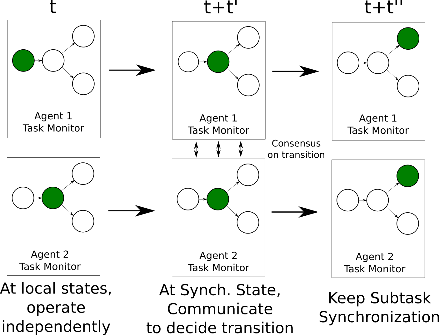
Figure 2: Overview of the DistSpectrl process for task synchronization. Branching in the task monitor diagram denotes potential non-deterministic choices between future tasks (such as in $\mathbf{\phi_{ex}}$). Left to right represents the order of policy actions over a trajectory. Green states represent the current monitor state of that agent.

6 Sub-task Synchronization

Importance of Task Synchronization

Consider the following example specification:

$$\phi_{1a}^{\prime}=\mathtt{reach}_{lo}(P)\ \mathtt{or}\ \mathtt{reach}_{gl}(Q)$$

where $P,Q$ are some goals. To ensure flexibility with respect to the possible acceptable rollouts within $\phi_{1a}^{\prime}$, the individual agent policies $\pi^{i}$ are learnable and the task transition chosen is dependent on the agent-specific observations. This flexibility between agents however, adds an additional possible failure method in achieving a global specification - if even a single agent attempts to fulfill the global objective while the others decide to follow their local objectives, the specification would never be satisfied.

Identifying Synchronization States

As emphasized above, task synchronization is an important aspect of deploying these composite task monitors in the Markov game $\mathcal{M}_{g}$ with specification $\phi$. We show the existence of a subset of monitor states $\mathtt{Sync}\in Q$ where in order to maintain task synchronization, agents simply require a consensus on which monitor transition $\delta=(q,\sigma,u,q^{\prime})$ to take. If we use $Q_{g}$ to symbolize the set of global monitor states, viz. all $q\in Q$ such that $\exists(q,\sigma_{g},u_{g},q^{\prime})\in\Delta_{g}$, then we see that $Q_{g}\subseteq\mathtt{Sync}$. A valid choice for $q\in\mathtt{Sync}$ with $q\notin Q_{g}$ is all branching states in the graph of $M_{\phi}$ with a set refinement presented in the Appendix (Sec. 0.D).

During training, we enforce the condition that when an agent $i$ has monitor state $q_{t}^{i}\in\mathtt{Sync}$, it must wait for time $t_{1}>t$ such that $q_{t_{1}}^{j}=q_{t}^{i}~{}\forall j\in\mathcal{N}$ and then choose a common transition as the other agents. This is done during the centralized training phase by sharing the same transition between agents based on a majority vote.

7 Multi-Agent Specification Properties

Consider a specification $\phi$ and let $\mathcal{N}=\{1,\ldots,N\}$ be the set of all agents with $\zeta_{m}$ being a trajectory sampled from the environment. $\phi(\zeta_{m},n)$ is used to denote that the specification is satisfied on $\zeta_{m}$ for the set of agents $n\subseteq\mathcal{N}$ (i.e. $\llbracket\phi(\zeta_{m},n)\rrbracket==\mathtt{True}$).

MA-Distributive

Many specifications pertaining to MA problems can be satisfied independent of the number of agents. At its core, we have the condition that a specification being satisfied with respect to a union of two disjoint sets of agents implies that it can be satisfied on both sets independently. Namely if $n_{1},n_{2}\subset\mathcal{N}$ with $n_{1}\cap n_{2}=\emptyset$ then an MA-Distributive specification satisifies the following condition:

$$\phi(\zeta_{m},n_{1}\cup n_{2})\implies\phi(\zeta_{m},n_{1})\land\phi(\zeta_{m},n_{2})$$

MA-Decomposable

Certain specifications satisfy a decomposibility property particular to multi-agent problems that can help in scaling with respect to the number of agents.

Say $\exists\ k\in\{1,\ldots,N-1\}$ such that

$$\phi(\zeta_{m},\mathcal{N})\implies\phi_{k}(\zeta_{m},\mathcal{N})=\bigwedge\limits_{j\in\{1,\ldots,J\}}\phi(\zeta_{m},n_{j})$$

where

$$n_{j}\subset\mathcal{N}\ ,\ k\leq|n_{j}|<N\ ,\ J=\lfloor\frac{N}{k}\rfloor\ ,\ \bigcap\limits_{j}n_{j}=\emptyset\ ,\ \bigcup\limits_{j}n_{j}=\mathcal{N}$$

with $\lfloor\rfloor$ representing the floor function. Each $n_{j}$ is a set of at least $k$ unique agents and $\{n_{j}\}_{j}$ forms a partition over $\mathcal{N}$.

We then call the specification $\phi$ MA-Decomposable with decomposibility factor $k$. Here $\phi_{k}$ can be thought of as a means to approximate the specification $\phi$ to smaller groups of agents within the set of agents $\mathcal{N}$. Provided we find a value of $k$, we can then use this as the basis of our MA-Dec scaling method to significantly improve training times for larger numbers of agents.

Theorem 7.1

(Proof in Appendix Sec. 0.F.) All MA-Distributive specifications are also MA-Decomposable with decomposability factors $k\in\mathbb{Z}^{+},1\leq k<N$.

Notably all compositions of $\mathtt{reach}_{gl}$ and $\mathtt{reach}_{lo}$ within our language are MA-Distributive and are thus MA-Decomposable with factor $k=2$. This is far from a general property however, as one can define specifications on $N$ robots such as $\mathtt{achieve}$("collect $x$ fruits") where each robot can carry at most $x/N$ fruits . In this case, no single subset of agents can satisfy the specification as the total capacity of fruits would be less than $x$ and the specification is neither MA-Distributive nor MA-Decomposable.

8 Algorithm

Training

Agents learn $\pi^{i}(s^{i},v^{i},q^{i})=(a^{i},\delta^{i})$ on the augmented Markov game $\mathcal{M}_{g}^{\prime}$ where $s^{i},v^{i},q^{i}$ are agent-specific state, register value and task monitor state respectively. Since training is centralized, all agent task monitors receive the same global state. Based on our discussion in Sec. 6, if an agent is in any given global monitor state, we wait for other agents to enter the same state, then do the $\arg\max$ task transition for all agents in the same state. In addition, at the synchronization states (Sec. 6), we perform a similar process to select the task transition. These trained augmented policies are then projected into policies that can act in the original $\mathcal{M}_{g}$.

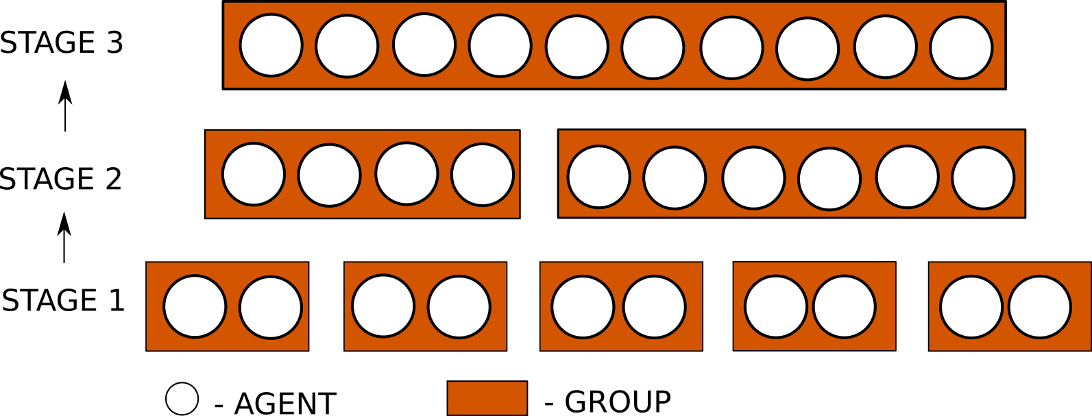
Figure 3: Example MA-Dec Scaling Process with $N=10,k=2,f=2$ on an MA-Decomposable spec $\phi$ with decomposability factor $2$. At Stage 1, $g_{1}=2$ to start with 5 groups. Next $g_{2}=fg_{1}=4$ which forms 2 groups. Finally at Stage 3, $g_{3}=fg_{2}=8$ which forms one group ($\mathcal{N}$).

Scaling MA-Decomposable Specifications

Our algorithm for scaling based off the MA-Decomposable property is shown in Alg. 1 (refer Appendix) and we name it MA-Dec scaling. Essentially, we approximate the spec. $\phi$ by first independently considering smaller groups within the larger set of agents $\mathcal{N}$ and try to obtain a policy satisfying $\phi$ on these smaller groups. By progressively making the group sizes larger over stages and repeating the policy training process while continuing from the previous training stage’s policy parameters , we form a curriculum that eases solving the original problem $\phi$ on all agents $\mathcal{N}$.

In Fig. 3 we demonstrate MA-Dec scaling for $N=10$ agents on a spec. $\phi$ which is MA-Decomposable with decomposability factor $2$. For this example we set the scaling parameters $k=2$ and $f=2$. Initially we have a min. group size $g_{1}=2$ and this is changed to $g_{2}=4$ and $g_{3}=8$ from setting the scaling factor. We increment the stage number every time all the groups of a stage have satisfied the entire specification $\phi$ w.r.t. their group. While separating training into stages, agents must be encouraged to move from stage $i$ to stage $i+1$. To ensure this, we need to scale rewards based on the stage. We chose a simple linear scaling where for stage number $i$ and time step $t$, each agent receives reward $r_{i,t}=ic_{k}+CTM_{i,t}$ where $CTM_{i,t}$ is the original composite task monitor reward at stage $i$ and $c_{k}\in\mathbb{R}$ is a constant. By bounding the reward terms such that rewards across stages are monotonically increasing $(r_{i,t}<r_{i+1,t^{\prime}})$ we can find a suitable $c_{k}$ to be $(2D+1)C_{u}$ (refer Appendix Sec. 0.B) where the terms are the same as in Eq. 1.

From setting the initial min. group size $g_{1}$ and scaling factor $f$, we get the total number of learning stages ($T_{s}$) as $T_{s}=\lfloor\log_{f}(N)-\log_{f}(k)\rfloor=\mathcal{O}(\log_{f}(N))$. We build the intuition behind why MA-Dec scaling is effective in the Appendix (Sec. 0.B), by describing it as a form of curriculum learning.

Deployment

Policies are constructed to proceed with only local information ($s^{i},v^{i},q^{i}$). Since we cannot share the whole system state with the agent policies during deployment yet our composite task monitor requires access to this state at all times, we allow the following relaxations: 1) Global predicates $\sigma_{g}(\bar{s},v)$ enabling task monitor transitions need global state and access it during deployment. 2) Global register updates $u_{g}(\bar{s},v)$ are also a function of global state and access it during deployment.

In order to maintain task synchronization, agents use a consensus based communication method to decide task monitor transitions at global and synchronization states. If agents choose different task transitions at these monitor states, the majority vote is used as done during training.

9 Experiment Setup

Our experiments aim to validate that the use of a distributed task monitor can achieve synchronization during the deployment of multiple agents on a range of specifications.

In addition, to emphasize the need for distribution of task monitors to alleviate the state space explosion caused by mixing local and global specifications, we include experiments with Spectrl applied to a centralized controller.

Lastly, we provide results showing the efficacy of the MA-Dec scaling approach for larger numbers of agents when presented with a specification that satisfies the MA-Decomposability property (Sec. 7).

As a baseline comparison, we also choose to run our algorithm without giving policies access to the monitor state (no_mon). These are trained with the same shaped reward as DistSpectrl. We also provide a Reward Machine baseline (RM) for $\phi_{1}$ with continuous rewards since $\phi_{1}$ is similar to the ’Rendezvous’ specification in [13].

Environment

Our first set of experiments are done on a 2D Navigation problem with $N=3$ agents. The observations ($\mathcal{S}\in\mathbb{R}^{2}$) used are coordinates within the space with the action space ($\mathcal{A}\in\mathbb{R}^{2}$) providing the velocity of the agent.

The second set of experiments towards higher dimension 3D benchmarks, represent particle motion in a 3D space. We train multiple agents ($N=3$) in the 3D space ($\mathcal{S}\in\mathbb{R}^{3}$) with a 3D action space ($\mathcal{A}\in\mathbb{R}^{3}$) to show the scaling potential of our framework.

The final set of experiments were on a modern discrete-action MARL benchmark built in Starcraft 2 [15] with $N=8$ agents (the "8m" map). Each agent has 14 discrete actions with a state space $\mathcal{S}\in\mathbb{R}^{80}$ representing a partial view of allies and enemies.

Algorithm Choices

For the scaling experiments (Fig. 6) we used the 2D Navigation problem with horizon $T=500$ and the scaling parameters $k=2$ and $f=2$. We also choose a version of PPO with a centralized Critic to train the augmented Markov Game noting that our framework is agnostic to the choice of training algorithm. The current stage is passed to the agents as an extra integer dimension. For other experiments we chose PPO with independent critics as our learning algorithm. Experiments were implemented using the RLLib toolkit [9].

Specifications

(2D Navigation) The evaluated specifications are a mix of local and global objectives. The reach predicates have an error tolerance of 1 (the $L_{\infty}$ distance from the goal).

(i) $\phi_{1}=\mathtt{reach_{gl}}(5,0);\mathtt{reach_{gl}}(0,0)$ , (ii) $\phi_{2}=\phi_{1};\mathtt{reach_{gl}}(3,0)$

(iii) $\phi_{3}=\mathtt{reach_{lo}}(5,0);\mathtt{reach_{gl}}(0,0);\mathtt{reach_{gl}}(3,0)$

(iv) $\phi_{4}=\left[\mathtt{reach_{lo}}(3,0)\ \mathtt{or}\ \mathtt{reach_{lo}}(5,10)\right];\phi_{3}$

(SC2) $\phi_{sc}$ represents ’kiting’ behaviour and is explained further in the Appendix (Sec. 0.E). $\phi_{sc}=\phi_{sc_{a}};\phi_{sc_{a}};\phi_{sc_{a}}$ where $\phi_{sc_{a}}=\mathtt{away\_from\_enemy}_{gl};\mathtt{shooting\_range}_{lo};$

(3D Environment ) $\phi_{a}=\mathtt{reach_{lo}}(5,0,0);\mathtt{reach_{gl}}(0,0,0);\mathtt{reach_{gl}}(3,0,0)$ is the specification considered within X-Y-Z coordinates.

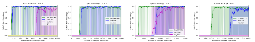
Figure 4: Satisfaction percentages on specifications $\phi_{1}$,$\phi_{2}$,$\phi_{3}$ and $\phi_{4}$ with $N=3$ agents. The shaded regions show the maximum and minimum achieved over 5 separate evaluation runs

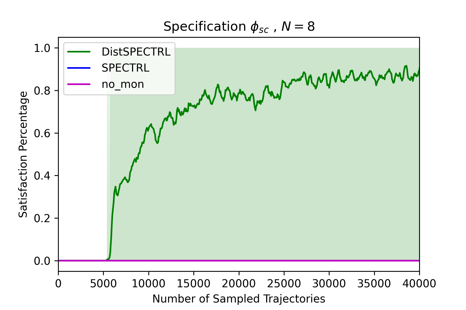
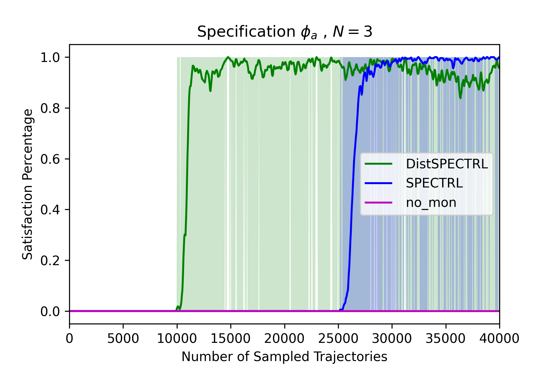
Figure 5: Specification satisfaction percentages (left) for the StarCraft 2 specification $\phi_{sc}$ with $N=8$ agents and (right) for the 3D Navigation experiments on specification $\phi_{a}$.

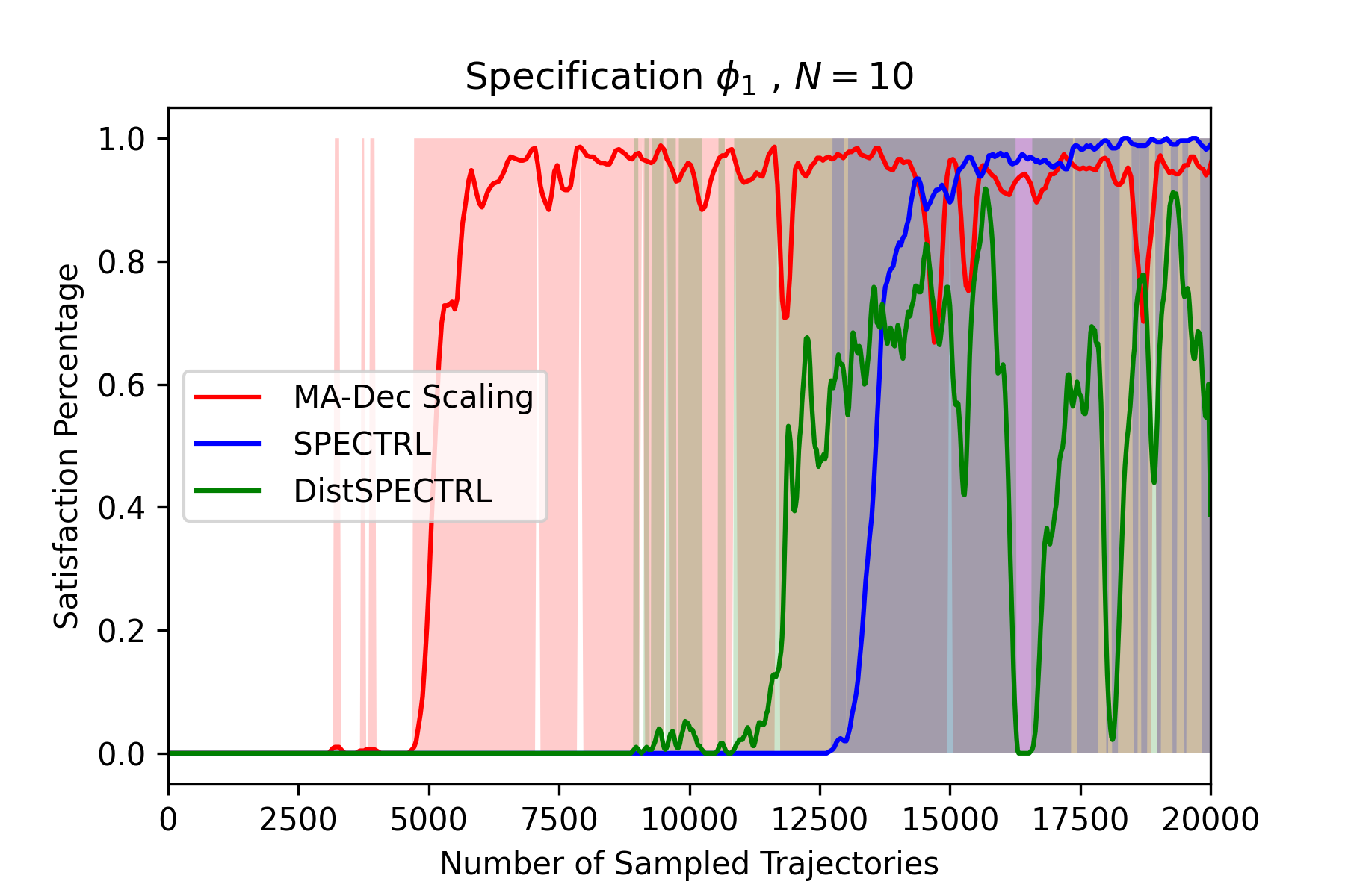
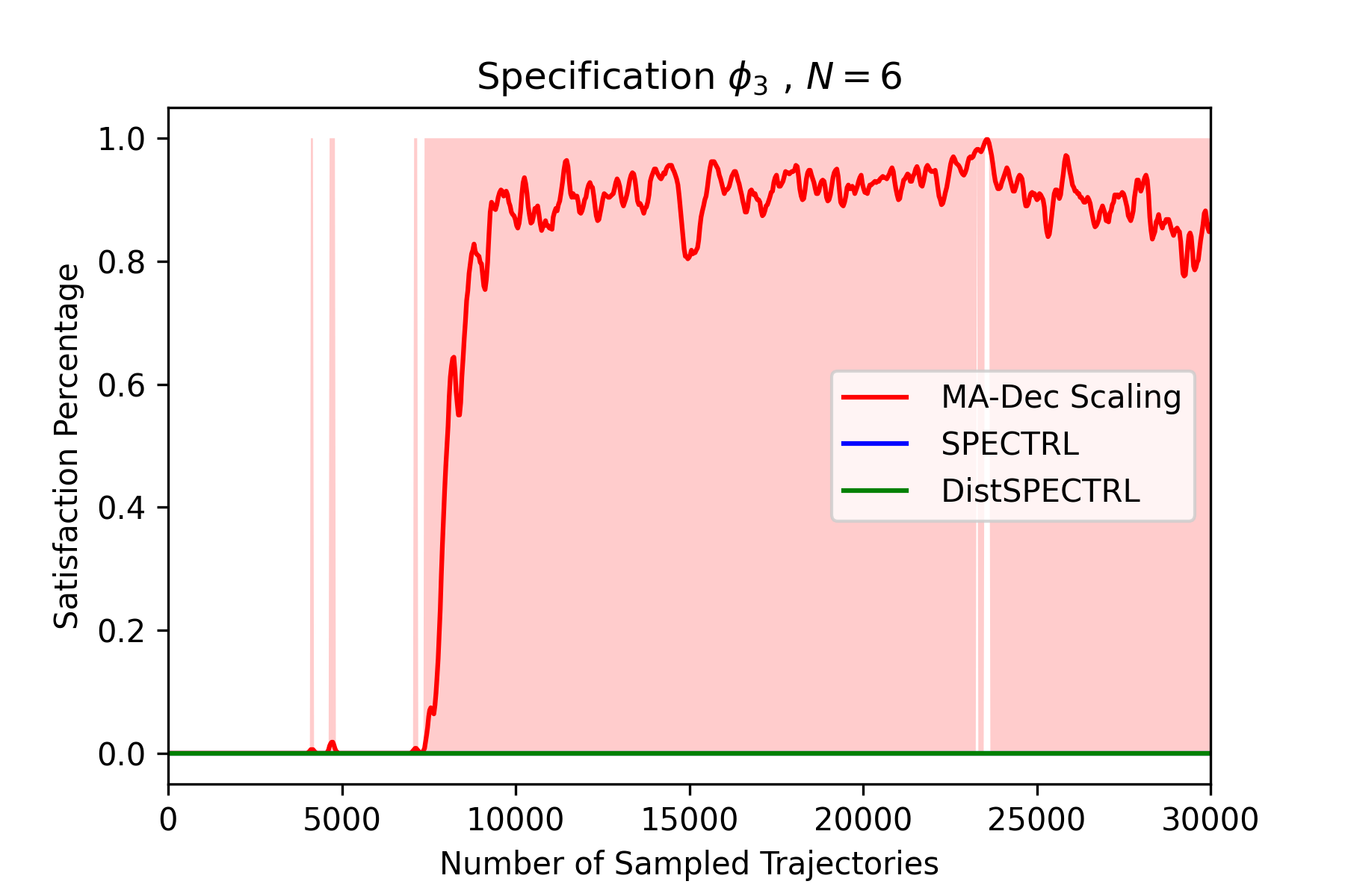
Figure 6: Specification satisfaction percentages for $N=10$ agents on $\phi_{1}$ (left) and $N=6$ agents on $\phi_{3}$ (right) comparing the MA-Dec scaling (red) to centralized Spectrl (blue) and vanilla DistSpectrl (green) i.e. without scaling enhancements.

Table 1: Specification satisfaction percentages on convergence for Fig.4,5

Spec.	DistSpectrl	no_mon	Spectrl
$\phi_{1}$	99.62	91.17	100.00
$\phi_{2}$	99.05	00.00	97.38
$\phi_{3}$	97.59	94.77	96.81
$\phi_{4}$	97.31	00.00	90.78
$\phi_{a}$	98.49	00.00	99.60
$\phi_{sc}$	86.79	00.00	00.00

Table 2: Specification satisfaction percentages on convergence for Fig.6, (Scaling to more Agents)

Spec. $/$ # Agents	MA-Dec	DistSpectrl	Spectrl
$\phi_{3}/N$ =6	94.09	0.00	0.00
$\phi_{1}/N$ =6	97.83	80.67	98.96
$\phi_{1}/N$ =10	97.03	72.30	99.28

10 Results

Handling Expressive Specifications

The experiments in Fig. 4 demonstrate execution when the task monitor predicates have access to the the entire system state. This provides agents with information sufficient to calculate global predicates for task monitor transitions. The overall satisfaction percentage is reported with the value $0$ being an incomplete task to $1.0$ being the entire specification satisfied.

While Spectrl has often been shown to be more effective [5, 6] than many existing methods (e.g. RM case) for task specification, the further utility of the monitor state in enhancing coordination between agents is clearly evident in a distributed setting. The task monitor state is essential for coordination as our baseline no_mon is often unable to complete the entire task (even by exhaustively going through possible transitions) and global task completion requires enhanced levels of synchronization between agents.

From Table 9 we see that upon convergence of the learning algorithm, the agent is able to maintain a nearly 100% task completion rate for our tested specifications, a significant improvement in comparison to the no_mon case, showing the importance of the task monitor as part of a multi-agent policy.

Benefits of Distribution Over Centralization

The centralized Spectrl graphs (blue curves in Figs. 4, 5, 6) show that while distribution may not be necessary for certain specifications with few local portions (e.g. $\phi_{2}$), concatenating them will quickly lead to learning difficulties with larger number of agents (Fig. 5, $\phi_{sc}$ and Fig. 6, $\phi_{3}$). This difficulty is due in large part to state space explosion of the task monitor in these cases as is apparent by the significantly better performance of our distributed algorithm. We also remind the reader that a centralized algorithm is further disadvantageous in MARL settings due to the added synchronization cost between agents during deployment.

Scaling to Larger State Spaces

The results in Fig. 5 show promise that the DistSpectrl framework can be scaled up to larger dimension tasks as well. The 3D environment results exhibits similar behavior to the 2D case with the no_mon showing difficulty in progressing beyond the local tasks in the larger state space with sparser predicates. The $\phi_{sc}$ results also show promise in defining relevant predicates and achieving general specifications for modern MARL benchmarks.

Scaling to More Agents

Table 9 and Fig. 6 demonstrate the benefits of MA-Dec scaling for larger $N$ when presented with an MA-Decomposable specification. At smaller ranges of $N$ as well as less complex combinations of mixed and global objectives, the effect of MA-Dec scaling is less pronounced. We observe that the stage based learning is crucial for a even simple mixed specification like $\phi_{3}$ with as little as $N=6$ agents.

11 Related Work

Multi-agent imitation learning [17, 7, 23] uses demonstrations of a task to specify desired behavior. However in many cases, directly being able to encode a specification by means of our framework is more straightforward and removes the need to have demonstrations beforehand. Given demonstrations, one may be able to infer the specification [21] and make refinements or compositions for use in our framework.

TLTL[8] is another scheme to incorporate temporal logic constraints into learning enabled controllers, although its insufficiency in handling non-Markovian specifications led us to choose Spectrl as the basis for our methodology. Reward Machines (RMs) [19, 2, 18] are an automaton-based framework to encode different tasks into an MDP. While RMs can handle many non-Markovian reward structures, a major difference is that Spectrl starts with a logical temporal logic specification and includes with the automaton the presence of memory (in the form of registers capable of storing real-valued information). Recent work [6] shows the relative advantages Spectrl-based solutions may have over a range of continuous benchmarks.

Concurrent work has introduced the benefits of a temporal logic based approach to reward specification [4]. While experimental results are not yet displayed, the convergence guarantees of the given algorithm are promising. Since we use complex non-linear function approximators (neural networks) in our work, such guarantees are harder to provide. Reward Machines have also been explored as a means of specifying behavior in multi-agent systems [13] albeit in discrete state-action systems that lend themselves to applying tabular RL methods such as Q-learning. One may extend this framework to continuous systems by means of function approximation but to the best of our knowledge, this has not been attempted yet. Similar to our synchronization state, the authors use a defined local event set to sync tasks between multiple agents and requires being aware of shared events visible to the other agents.

In the same spirit as our stage-based approach, transferring learning from smaller groups of agents to larger ones has also been explored [22]. Lastly, while we chose PPO to train the individual agents for its simplicity, our framework is agnostic to the RL algorithm used and can be made to work with other modern multi-agent RL setups [11, 3] for greater coordination capabilities.

12 Conclusion

We have introduced a new specification language to help detail MARL tasks and describe how it can be used to compile a desired description of a distributed execution in order to achieve specified objectives. Our framework makes task synchronization realizable among agents through the use of: 1) Global predicates providing checks for task completion that are easily computed, well-defined and tractable; 2) A monitor state to keep track of task completion; and 3) Synchronization states to prevent objectives from diverging among agents.

Acknowledgements

This work was supported in part by C-BRIC, one of six centers in JUMP, a Semiconductor Research Corporation (SRC) program sponsored by DARPA.

Appendix 0.A Global Task Monitor Construction

We refer readers to the local specification compilation rules of Spectrl (defined in their Appendix). We highlight the main differences with mixed objectives here.

For a specification $\phi$ let $Q_{g}$ the set of states with global predicates in $\phi$. Note that $Q_{g}\subseteq\mathtt{Sync}$ as mentioned in Sec 6. Here we consider a $\phi$ to be global if it contains any global predicates.

$\mathtt{achieve}~{}b$ when $b$ is a global predicate

Add both states to global states $Q_{g}$.

$\phi_{1};~{}\phi_{2}$ when $\phi_{2}$ is global

If $\phi_{2}$ has an initial global state or $(q_{0})_{\phi_{2}}\in(\mathtt{Sync})_{\phi_{2}}$ then the transition from the final state of $\phi_{1}$ to $\phi_{2}$ is also global. If $q_{a}\in F_{\phi_{1}}$ then $q_{a}\in Q_{g}$.

$\phi_{1};~{}\phi_{2}$ when $\phi_{1}$ is global

It is the same as the local case with $Q_{g}=(Q_{g})_{\phi_{1}}$

$\phi_{1};~{}\phi_{2}$ when both $\phi_{1},\phi_{2}$ are global

It is the same as the local case with $Q_{g}=(Q_{g})_{\phi_{1}}\cup(Q_{g})_{\phi_{2}}$

$\phi_{1}\mathtt{or}~{}\phi_{2}$ when $\phi_{2}$ is global

Without loss of generality, if $\phi_{2}$ contains global states then the common start state (as part of the compilation rules of $\mathtt{or}$) is a synchronization state. $Q_{g}=(Q_{g})_{\phi_{1}}\cup(Q_{g})_{\phi_{2}}$.

Appendix 0.B Scaling MA Specifications

MA-Dec Scaling can be thought of as a form of curriculum learning for MA-Distributive specifications. We progressively narrow down the valid space of parameters that satisfy the specification $\phi_{k}$ by increasing the value of $k$ by a positive integer factor $f>1$. Consider a set of $N=10$ agents and an MA-Distributive specification $\phi$. $\phi$ is also MA-Decomposable with factor $8$ by Thm. 7.1. Since the spec. is MA-Distributive as well $\phi_{8}(\eta,\mathcal{N})\implies\phi_{4}(\eta,\mathcal{N})\implies\phi_{2}(\eta,\mathcal{N})$.

Intuitively, as shown in Fig. 7, the policy parameter $\Pi_{\theta}$ satisfying $\phi_{8}$ will also satisfy $\phi_{4}$ and $\phi_{2}$ as groups of 8 agents can either be considered two groups of 4 agents or four groups of 2 agents.

Thus we position the parameter spaces as shown, and in the first stage attempt to find a parameter within the largest region satisfying $\phi_{2}(\mathcal{N})$. As the learning progresses, the curriculum narrows down the desired search space until we obtain the parameters satisfying the specification $\phi(\mathcal{N})$.

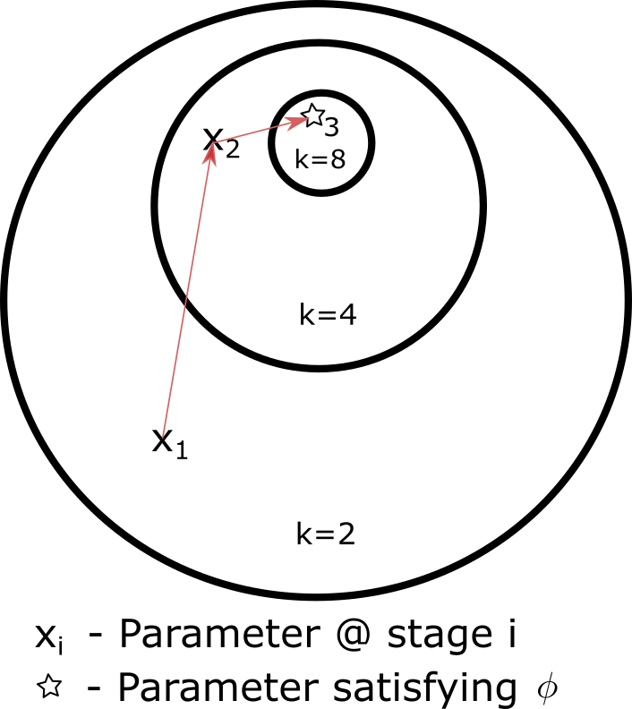
Figure 7: Scaling intuition for $N=10,k=2,f=2$. We represent the policy parameter space and the respective placement of parameters that satisfy $\phi_{k}$ for various values of $k$. The arrows show the direction we proceed searching for parameters in our scaling process.

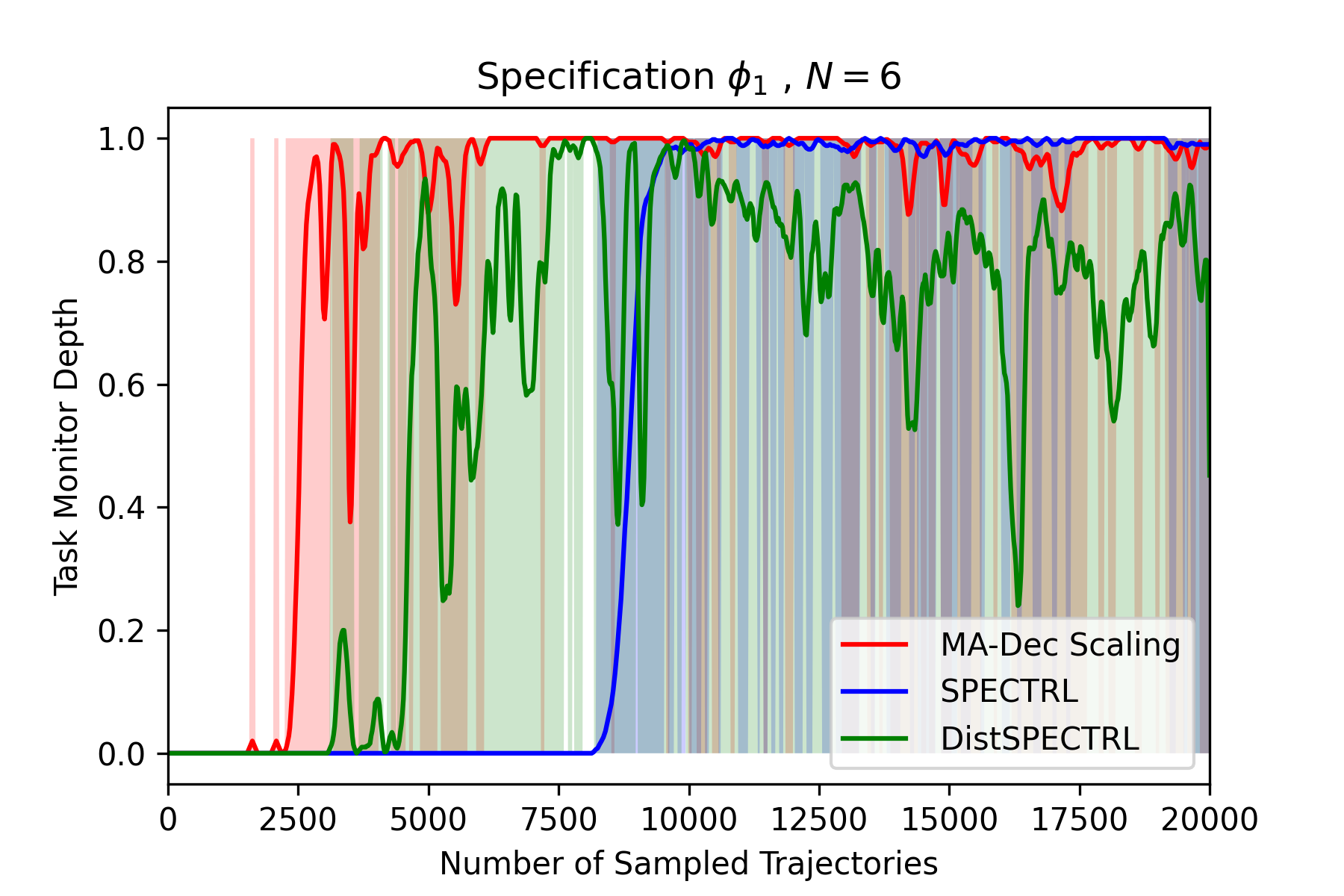
Figure 8: Specification satisfaction percentages for $N=6$ agents on $\phi_{1}$ comparing the MA-Dec scaling method (red) to centralized Spectrl (blue) and vanilla DistSpectrl (green).

Given Specification $\phi$ that is MA-Decomposable with factor $k$ and agent set $\mathcal{N}$ of $N$ agents.

Given a function $\texttt{train}(\phi,n_{j})$ that trains a policy satisfying $\phi$ (up to a performance metric) from a previous set of policy parameters for the group of agents $n_{j}$.

Function set_groups($g$, $\mathcal{N}$):

       // $g\in\mathbb{Z}^{+}$ i.e. an integer $g\geq 1$

      // Makes partition of $\mathcal{N}$ with minimum group size $g$

      if $g>|\mathcal{N}|$ then

            return $\{\mathcal{N}\}$

       else

             Initialize $j=1,J=\lfloor\frac{N}{g}\rfloor$

            foreach $a\in\mathcal{N}$ do

                   if $|n_{j}|<g\ \mathtt{or}\ j==J$  then

                        $n_{j}\leftarrow n_{j}\cup{a}$

                   else

                         $j\leftarrow j+1$

                        $n_{j}=\{\}$

                  

             end foreach

            

            return $\{n_{j}\}_{j}$

      

Initialize Agent Policies $\Pi$, $i=1$, $g_{1}=k$

Initialize $\{n_{j}\}_{j}=$set_groups($g_{1}$, $\mathcal{N}$)

while $|n_{1}|\leq|\mathcal{N}|$ do

       foreach $n_{j}\in\{n_{j}\}_{j}$ do

             Run ${\Pi}\leftarrow\texttt{train}(\phi,n_{j})$ independently of agents $\mathcal{N}\setminus n_{j}$ updating the policies of $n_{j}$.

       end foreach

      

      $g_{i+1}=fg_{i}$.

      if $g_{i+1}>|\mathcal{N}|$ then

             // Already reached Final Stage with $n_{1}==\mathcal{N}$

            return

      

      $\{n_{j}\}_{j}\leftarrow$ set_groups($g_{i+1}$, $\mathcal{N}$)

      $i\leftarrow i+1$

end while

Algorithm 1 MA-Dec Scaling

Calculating Scaling constant $\mathbf{c_{k}}$

We want all rewards at stage $i$ to be less than the rewards at stage $i+1$ to prevent local optima from arising where an agent is not incentivized to progress to the next stage. Assuming that the final reward at all stages is also upper bounded by $C_{u}$ (as is $\alpha$).

$$r_{i,t}\leq r_{i+1,t^{\prime}} ~{}\forall t,t^{\prime}$$

$$\implies ic_{k}+CTM_{i,t}\leq (i+1)c_{k}+CTM_{i+1,t^{\prime}}$$

$$\implies\max(ic_{k}+CTM_{i,t})\leq \min((i+1)c_{k}+CTM_{i+1,t^{\prime}})$$

Since $c_{k}\in\mathbb{R}$ is a constant we get

$$\max(CTM_{i,t})-\min(CTM_{i+1,t^{\prime}})\leq c_{k}$$

$$\implies C_{u}-(-2DC_{u})\leq c_{k}$$

Thus a suitable $c_{k}$ is $(2D+1)C_{u}$.

Appendix 0.C Implementation

Computational resources

All experiments were run on a Intel Xeon Gold 2.10 Ghz 64-core machine with 252 GB of RAM. Individual experiments used no more than 16 cores at a time with experiments involving a hyperparameter search taking 2 cores each.

Hyperparameters

A single 2 layer neural network with 256 nodes each and a $\tanh$ activation function was used. The learning rate was varied from $1\times 10^{-3}$ to $1\times 10^{-5}$ over $2\times 10^{7}$ iterations.

We used a grid search on hyperparameters for all experiments.

Table 3: Hyperparameters used for grid search

Hyperparameter	Ranges
Batch Size	$[10000,20000]$
Initial Learning Rate	$[10^{-3},10^{-4},10^{-5}]$
Entropy Coefficient	$[0,0.00176]$

Metrics

The specification satisfaction is reported with value from $0$ being no sub-task completed to $1.0$ being the entire specification satisfied. For more details on the compilation rules we refer readers to Sec. 0.A.

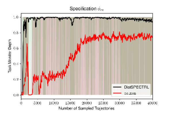
Figure 9: Specification satisfaction percentages for the task monitor shown in Fig. 1 with $\phi_{ex}=\mathtt{reach}_{gl}(10,10);\mathtt{or}\ \left[\mathtt{reach}_{lo}(3,0);\left[\mathtt{reach}_{lo}(10,10)\ \mathtt{or}\ \mathtt{reach}_{gl}(5,0)\right]\right]$.

Appendix 0.D Subtask Synchronization

Another example to further strengthen this notion of task synchronization is

$$\phi_{2a}^{\prime}=\left[\mathtt{reach}_{lo}(P);\mathtt{reach}_{gl}(Q)\ \right]\mathtt{or}\ \left[\mathtt{reach}_{lo}(P^{\prime});\mathtt{reach}_{gl}(Q^{\prime})\ \right]$$

Here, if an agent assumed that it only needed to choose between the two local objectives $\mathtt{reach}_{lo}(P)$ and $\mathtt{reach}_{lo}(P^{\prime})$ and not look further into the future for the presence of global objectives, a task mismatch would occur between agents who are in different branches of the task monitor i.e. the sub-specification $\left[\mathtt{reach}_{lo}(P);\mathtt{reach}_{gl}(Q)\ \right]$ vs. $\left[\mathtt{reach}_{lo}(P^{\prime});\mathtt{reach}_{gl}(Q^{\prime})\ \right]$. We see that global objectives deeper in the sequence of specifications require prior synchronization to reaching the stage just before task completion. Thus, we see there is a marked need for task synchronization among agents as specifications become increasingly complex.

The identification of local synchronization states $q\in\mathtt{Sync}$ , where $q\notin Q_{g}$ is as follows:

1. Select all branching states in the graph of $M_{\phi}$.

2. Remove those with all branches local and disconnected.

   That is, all monitor states in these branches that only have local transitions $\delta_{l}$.

3. Remove all those whose branches rejoin at some state (the rejoin point) and have all paths from branching state to the rejoin point not include any global monitor states.

   That is, if we consider only the subgraph of $M_{\phi}$ starting from the branching state, the rejoin point should have no ancestors which are global monitor states.

Appendix 0.E Environments

2D Environment

The environment follows first order dynamics in a 2D space ($\mathcal{S}\in\mathbb{R}^{2}$). The action space ($\mathcal{A}\in\mathbb{R}^{2}$) provides the velocity of the agent in the space. Agents are initialized in a line below their reference goals at a Y-coordinate uniformly sampled between $(2,3)$.

3D Environment

The environment follows first order dynamics in a 3D space ($\mathcal{S}\in\mathbb{R}^{3}$). The action space ($\mathcal{A}\in\mathbb{R}^{3}$) provides the velocity of the agent in the space. Agents are initialized below the goal in the X-Y plane and with a random Y,Z coordinate uniformly sampled between $(2,3)$.

StarCraft 2

Starcraft 2 [15] experiments used the "8m" map with 8 controllable marines and 8 enemy AI-controlled marines. Each agent had state space $\mathcal{S}\in\mathbb{R}^{80}$ and 14 discrete actions. $\mathtt{away\_from\_enemy}$ defines a predicate that is true when the agent cannot be shot by the enemy. $\mathtt{shooting\_range}$ defines a predicate that is true when the agent can shoot the enemy (but can also be shot as well). $\mathtt{away\_from\_enemy}_{gl}$ being true implies that all the agents are together away from the enemy at once (in a synchronized manner).

To define these predicates we make use of two indicators provided by the Starcraft 2 environment. The first being $\mathtt{shooting\_range\_ind}\in\{0,1\}$ which is 1 when the enemy within shooting range and 0 otherwise. The other is $\mathtt{dist\_to\_enemy}\in[0,1]$ being the normalized distance to an enemy which is 0 when the enemy is not visible (the observation radius is larger than the shooting range) .

The quantitative semantics of these new predicates are then

$$\llbracket\mathtt{away\_from\_enemy}\rrbracket_{q}= (1-\mathtt{shooting\_range\_ind})*(\epsilon)+$$

$$\mathtt{shooting\_range\_ind}*(\mathtt{dist\_to\_enemy}-\epsilon)$$

$$\llbracket\mathtt{shooting\_range}\rrbracket_{q}= (1-\mathtt{shooting\_range\_ind})*(-\epsilon)+$$

$$\mathtt{shooting\_range\_ind}*(\mathtt{dist\_to\_enemy}-\epsilon/10)$$

where $\epsilon\in[0,1]$ is a real-value representing the error tolerance set to 0.5 in the Starcraft experiments.

To augment our discrete action space Markov Game for the centralized SPECTRL comparison, we included an additional agent with access to the full system state. This centralized controller was used to choose between the available task monitor transitions.

Appendix 0.F Proofs

Proof of Theorem 5.1

The proof follows the exact outline as in Spectrl since the language composition and compilation rules are equivalent in the necessary steps. We repeat their arguments here for clarity. First, the following lemma follows by structural induction:

Lemma 1

For $\sigma\in\Sigma$, $\llbracket\sigma\rrbracket(s,v)=\mathtt{True}\iff\llbracket\sigma\rrbracket_{q}(s,v)>0$.

Next, let $G_{M}$ denote the underlying state transition graph of a task monitor $M$. Then,

Lemma 2

The task monitors constructed by our algorithm satisfy the following properties:

1. The only cycles in $G_{M}$ are self loops.

2. The finals states are precisely those states from which there are no outgoing edges except for self loops in $G_{M}$.

3. In $G_{M}$, every state is reachable from the initial state and for every state there is a final state that is reachable from it.

4. For any pair of states $q$ and $q^{\prime}$, there is at most one transition from $q$ to $q^{\prime}$.

5. There is a self loop on every state $q$ given by a transition $(q,\top,u,q)$ for some update function $u$ where $\top$ denotes the true predicate.

The first three properties ensure progress when switching from one monitor state to another. The last two properties enable simpler composition of task monitors. The proof follows by structural induction. Theorem 5.1 now follows by structural induction on $\phi$ and Lemmas 1 and 2.

Proof of Theorem 5.2

i) Let $\tilde{\zeta}_{m},\tilde{\zeta}_{m}^{\prime}$ be two augmented rollouts such that $\tilde{R}^{i}(\tilde{\zeta}_{m})>\tilde{R}^{i}(\tilde{\zeta}_{m}^{\prime})$.

• Case A. Both $\tilde{\zeta}_{m},\tilde{\zeta}_{m}^{\prime}$ end in final monitor states. Here $\tilde{R}^{i}_{s}(\tilde{\zeta}_{m})=\tilde{R}^{i}(\tilde{\zeta}_{m})>\tilde{R}^{i}(\tilde{\zeta}_{m}^{\prime})=\tilde{R}_{s}^{i}(\tilde{\zeta}_{m}^{\prime})$.

• Case B. $\tilde{\zeta}_{m}$ ends in a final monitor state but $\tilde{\zeta}_{m}^{\prime}$ does not. Here

  $$\tilde{R}_{s}^{i}(\tilde{\zeta}_{m})= \max_{k\leq j<T}\alpha(\bar{s}_{j},q^{i}_{T},v_{j})$$

  $$+2C_{u}(d_{q^{i}_{T}}-D)+C_{l}$$

  $$\leq \max_{k\leq j<T}\alpha(\bar{s}_{j},q^{i}_{T},v_{j})-2C_{u}+C_{l} (d_{q^{i}_{T}}-D\leq-1)$$

  $$\leq C_{l} (C_{u}\geq\alpha,C_{u}\geq 0)$$

  $$\leq \tilde{R}^{i}(\tilde{\zeta}_{m}) (C_{l}\leq\tilde{R}^{i}~{}\forall~{}i\in\mathcal{N})$$

  $$= \tilde{R}_{s}^{i}(\tilde{\zeta}_{m}) (q^{i}_{T}\in F)$$

• Case C. $\tilde{\zeta}_{m}$ ends in a non-final monitor state. Here $\tilde{R}^{i}(\tilde{\zeta}_{m})=-\infty$ and $\tilde{R}^{i}(\tilde{\zeta}_{m}^{\prime})=-\infty$ as well.

(ii) if $\tilde{\zeta}_{m}$ and $\tilde{\zeta}_{m}^{\prime}$ end in distinct non-final monitor states $q^{i}_{T}$ and $(q^{i}_{T})^{\prime}$ such that $d_{q^{i}_{T}}>d_{(q^{i}_{T})^{\prime}}$, then $\tilde{R}^{i}_{s}(\tilde{\zeta}_{m})\geq\tilde{R}^{i}_{s}(\tilde{\zeta}_{m}^{\prime})$.

Here the trajectories vary in only one agent’s monitor state.

$$\tilde{R}_{s}^{i}(\tilde{\zeta}_{m})= \max_{k\leq j<T}\alpha(\bar{s}_{j},q^{i}_{T},v_{j})+C_{l}$$

$$+2C_{u}(d_{q^{i}_{T}}-D)$$

$$\geq \max_{k\leq j<T}\alpha(\bar{s}_{j},q^{i}_{T},v_{j})+C_{l} (d_{q^{i}_{T}}\geq d_{q^{i}_{T}}^{\prime}+1)$$

$$+2C_{u}(d_{q^{i}_{T}}^{\prime}-D)+2C_{u}$$

$$\geq C_{u}+C_{l} (C_{u}>|\alpha|\implies C_{u}>-\alpha)$$

$$+2C_{u}(d_{q^{i}_{T}}^{\prime}-D)$$

$$\geq \max_{k\leq j<T}\alpha(\bar{s}_{j}^{\prime},(q^{i}_{T})^{\prime},v_{j}^{\prime})+C_{l} (C_{u}>\alpha)$$

$$+2C_{u}(d_{q^{i}_{T}}^{\prime}-D)$$

$$= \tilde{R}_{s}^{i}(\tilde{\zeta}_{m}^{\prime})$$

Proof of Theorem 7.1

Given $\phi$ being MA-Distributive, then for two disjoint sets of agents $n_{1},n_{2}\subset\mathcal{N}$

$$\phi(\zeta_{m},n_{1}\cup n_{2})\implies\phi(\zeta_{m},n_{1})\land\phi(\zeta_{m},n_{2})$$

Given a value $k\in\mathbb{Z}^{+},1\leq k<N$ we can create a group of agent sets $\{n_{j}\}_{j\in{1,\ldots,J}}$ forming a partition of $\mathcal{N}$ with minimum group size $k$ using the $\mathtt{set\_groups}(k,\mathcal{N})$ function in Alg.1. Now

$$\phi(\zeta_{m},\bigcup_{j\in{1,\ldots,J}}n_{j})\implies \phi(\zeta_{m},n_{1})\land\phi(\zeta_{m},\bigcup_{j\in{2,\ldots,J}}n_{j})$$

$$\implies \phi(\zeta_{m},n_{1})\land\phi(\zeta_{m},n_{2})\land\phi(\zeta_{m},\bigcup_{j\in{3,\ldots,J}}n_{j})$$

$$\implies \bigwedge\limits_{j\in\{1,\ldots,J\}}\phi(\zeta_{m},n_{j})$$

Thus $\phi$ is also MA-Decomposable with factors $k\in\mathbb{Z}^{+},1\leq k<N$.

References

- [1] Andrychowicz, M., Wolski, F., Ray, A., Schneider, J., Fong, R., Welinder, P., McGrew, B., Tobin, J., Pieter Abbeel, O., Zaremba, W.: Hindsight experience replay. In: NIPS (2017)
- [2] Camacho, A., Toro Icarte, R., Klassen, T.Q., Valenzano, R., McIlraith, S.A.: LTL and beyond: Formal languages for reward function specification in RL. In: IJCAI (2019)
- [3] Foerster, J., Farquhar, G., Afouras, T., Nardelli, N., Whiteson, S.: Counterfactual multi-agent policy gradients. In: AAAI (2018)
- [4] Hammond, L., Abate, A., Gutierrez, J., Wooldridge, M.: Multi-agent reinforcement learning with temporal logic specifications. In: AAMAS (2021)
- [5] Jothimurugan, K., Alur, R., Bastani, O.: A composable specification language for reinforcement learning tasks. In: NeurIPS (2019)
- [6] Jothimurugan, K., Bansal, S., Bastani, O., Alur, R.: Compositional reinforcement learning from logical specifications. In: NeurIPS (2021)
- [7] Le, H.M., Yue, Y., Carr, P., Lucey, P.: Coordinated MA imitation learning. In: ICML (2017)
- [8] Li, X., Vasile, C., Belta, C.: RL with temporal logic rewards. In: IROS (2017)
- [9] Liang, E., Liaw, R., Nishihara, R., Moritz, P., Fox, R., Goldberg, K., Gonzalez, J., Jordan, M., Stoica, I.: RLlib: Abstractions for distributed reinforcement learning. In: ICML (2018)
- [10] Lillicrap, T.P., Hunt, J.J., Pritzel, A., Heess, N., Erez, T., Tassa, Y., Silver, D., Wierstra, D.: Continuous control with deep reinforcement learning. In: ICLR (2016)
- [11] Lowe, R., Wu, Y., Tamar, A., Harb, J., Abbeel, P., Mordatch, I.: Multi-agent actor-critic for mixed cooperative-competitive environments. In: NIPS (2017)
- [12] Mania, H., Guy, A., Recht, B.: Simple random search of static linear policies is competitive for reinforcement learning. In: NeurIPS (2018)
- [13] Neary, C., Xu, Z., Wu, B., Topcu, U.: Reward machines for cooperative multi-agent reinforcement learning. In: AAMAS (2021)
- [14] Ng, A.Y., Harada, D., Russell, S.: Policy invariance under reward transformations: Theory and application to reward shaping. In: ICML (1999)
- [15] Samvelyan, M., Rashid, T., Schroeder de Witt, C., Farquhar, G., Nardelli, N., Rudner, T.G.J., Hung, C.M., Torr, P.H.S., Foerster, J., Whiteson, S.: Starcraft challenge. In: AAMAS (2019)
- [16] Schulman, J., Wolski, F., Dhariwal, P., Radford, A., Klimov, O.: Proximal policy optimization algorithms. CoRR (2017)
- [17] Song, J., Ren, H., Sadigh, D., Ermon, S.: Multi-agent generative adversarial imitation learning. In: NeurIPS (2018)
- [18] Toro Icarte, R., Klassen, T.Q., Valenzano, R., McIlraith, S.A.: Using reward machines for high-level task specification and decomposition in reinforcement learning. In: ICML (2018)
- [19] Toro Icarte, R., Klassen, T.Q., Valenzano, R., McIlraith, S.A.: Reward machines: Exploiting reward function structure in reinforcement learning. arXiv preprint arXiv:2010.03950 (2020)
- [20] Vardi, M., Wolper, P.: Reasoning about infinite computations. Information and Comp. (1994)
- [21] Vazquez-Chanlatte, M., Jha, S., Tiwari, A., Ho, M.K., Seshia, S.: Learning task specifications from demonstrations. In: NeurIPS (2018)
- [22] Wang, W., Yang, T., Liu, Y., Hao, J., Hao, X., Hu, Y., Chen, Y., Fan, C., Gao, Y.: From few to more: Large-scale dynamic multiagent curriculum learning. In: AAAI. No. 05 (2020)
- [23] Yu, L., Song, J., Ermon, S.: Multi-agent adversarial inverse RL. In: ICML (2019)