vKompth: A variable Comptonisation model for low-frequency quasi-periodic oscillations in black-hole X-ray binaries

Abstract

Low mass X-ray binaries (LMXBs) show strong variability over a broad range of time scales. The analysis of this variability, in particular of the quasi-periodic oscillations (QPO), is key to understanding the properties of the innermost regions of the accretion flow in these systems. We present a time-dependent Comptonisation model that fits the energy-dependent rms-amplitude and phase-lag spectra of low-frequency QPOs in black-hole (BH) LMXBs. We model the accretion disc as a multi-temperature blackbody source emitting soft photons which are then Compton up-scattered in a spherical corona, including feedback of Comptonised photons that return to the disc. We compare our results with those obtained with a model in which the seed-photons source is a spherical blackbody: at low energies the time-averaged, rms and phase-lag spectra are smoother for the disk-blackbody than for a blackbody, while at high energies both models give similar spectra. In general, we find that the rms increases with energy, the slope of the phase-lag spectrum depends strongly on the feedback, while the minimum-lag energy is correlated with the disc temperature. We fit the model to a 4.45-Hz type-B QPO in the BH LMXB MAXI J1438–630 and find statistically-better fits and more compatible parameters with the steady-state spectrum than those obtained with a blackbody seed-photons source. Furthermore, we successfully apply the model to the type-C QPO in the BH LMXB GRS 1915+105, and thus conclude that this variable-Comptonisation model reproduces the rms and phase-lags of both type B and C low-frequency QPOs in BH LMXBs.

1 Introduction

Low mass X-ray binaries (LMXB) are binary systems consisting of a compact object, a neutron star (NS) or a black hole (BH), accreting matter from a low-mass star. These sources present very high variability in their X-ray light curves over a broad range of time scales, from tens of milliseconds to years (Belloni & Motta, 2016; Méndez & Belloni, 2021). The analysis of the variability is important because it gives us information about the accretion process in these objects (van der Klis, 1994; Stella & Vietri, 1998; Ingram et al., 2009; Kara et al., 2019; Mastroserio et al., 2019; Reig & Kylafis, 2021; Wang et al., 2021).

Some BH-LMXBs are transient sources that during outburst describe a $q$ shape in the hardness-intensity diagram (HID) (Méndez & van der Klis, 1997; Homan et al., 2001; Belloni et al., 2005). We can identify different states in the HID during an outburst of a BH-LMXB: at the start of the outburst the source is in the low hard state (LHS), with a hard energy spectrum. As the outburst progresses, the source follows an almost vertical path in the HID, increasing its intensity and barely decreasing its hardness. Eventually, the source transitions to the hard-intermediate and soft-intermediate states (HIMS and SIMS respectively) where, at an essentially constant intensity, the spectrum softens until the source reaches the high soft state (HSS). In this state the energy spectrum is soft and the intensity decreases while the hardness remains more or less constant. Finally, the source returns to the LHS completing the $q$ shape in the HID.

The power density spectra (PDS) of LMXBs present narrow features at characteristic frequencies, called quasi-periodic oscillations (QPOs), which correspond to variability in the X-ray light curve on well-defined timescales, providing information about the innermost regions of the accretion flow (Ingram & Motta, 2020). A QPO is characterized by a centroid frequency, $\nu_{0}$, a full-width half maximum, $\mathrm{FWHM}$, an amplitude, and the energy-dependent phase lag. Low-frequency QPOs (LF QPOs) observed in BH-LMXBs can be classified into three types, A, B, and C, according to their strength, quality factor, $Q=(\nu_{0}/\mathrm{FWHM})$, fractional root mean square (rms) amplitude, the properties of the underlying broadband noise in the PDS, and the spectral state of the source (Belloni et al., 2005; Casella et al., 2005). Type-A LF QPOs are broad peaks with centroid frequencies around 8 Hz and weak variability; they have a quality factor $Q<3$ and appear in the HSS. Type-B QPOs are narrower than type-A QPOs and have centroid frequencies around 6 Hz and a $Q>6$; they display a relatively weak variability, $\approx 4\%$ rms, and are found in the soft-intermediate state in the HID, where the spectrum is dominated by the soft component. Type C QPOs are narrow and strong features that peak around a variable centroid frequency between 0.1-15 Hz; they have a $Q>10$ and are very frequent in the hard and hard-intermediate states, where the spectrum is dominated by a hard component.

In this paper we propose a model that explains the rms and lag spectra of the LF-QPOs in BH-LMXB. While in principle the model that we describe here would be applicable to the three types of QPOs, type-A QPOs are very weak and up to date there is no report of an rms or lag spectrum of this type of QPOs. Hence, we will focus on type-B and C QPOs.

The X-ray spectrum of a BH-LMXBs is usually fitted with three additive components: a soft component emitted by an optically thick, geometrically thin accretion disk (Shakura & Sunyaev, 1973), which dominates in the HSS, a hard component, produced in a plasma of highly energetic electrons (Sunyaev & Titarchuk, 1980), called the corona, that dominates in the LHS, and a reflection component (Fabian et al., 1989). The hard component is likely due to Comptonisation, which is the predominant interaction process between photons and hot electrons since it reproduces correctly the shape of the spectrum of X-ray sources at high energies (Sunyaev & Truemper, 1979; Kazanas et al., 1997). The corona may well be a component of the accretion flow (Ingram et al., 2009) or the base of an out-flowing jet (Giannios et al., 2004; Markoff et al., 2005; Reig & Kylafis, 2021)

For most QPOs in LMXBs, the variability increases with energy, reaching 20$-$30% around 30 keV (eg.: for kHz QPOs Berger et al. 1996; Méndez et al. 2001; Gilfanov et al. 2003, for HFQPOs in BHC Morgan et al. 1997; Belloni & Altamirano 2013, for type-C QPO Rodriguez et al. 2002; Yadav et al. 2016; Zhang et al. 2017; Zhang et al. 2020). At these energies, the contribution of the soft component to the X-ray spectrum is negligible; hence, the accretion disk alone cannot explain the rms amplitude behaviour. The recent measurements of a QPO up to $\sim$200 keV in MAXI J1820+070 (Ma et al., 2020) shows that reflection cannot explain the rms spectrum of this QPO because, even though reflection peaks around 20 keV, it decays at higher energies and it is unable to produce the variability observed up to 150-300 keV. Thus, the only possible explanation of the high rms amplitude of QPOs at (very) high energies is that the corona is leading the variability, either producing it directly or amplifying the oscillations produced in the accretion disk at different energy bands (Sobolewska & Życki, 2006).

Inverse Compton scattering naturally leads to a hard lag (the hard photons lag behind the soft ones) because the travel path inside the corona and the energy of a photon increase each time the photon is inverse-Compton scattered; because of this high-energy photons that suffered many scatterings escape the corona after low-energy photons that suffered less or no scatterings (Miyamoto et al., 1988). Some up-scattered photons may return to the disk and be re-emitted later. This mechanism, called feedback, produces a soft lag, where the less energetic photons are those that arrive later (Lee & Miller, 1998).

Several papers proposed that the radiative properties of the variability in NS-LMXBs are due to the oscillation of thermodynamic properties of the corona or of the soft photon source (Lee & Miller, 1998; Lee et al., 2001; Kumar & Misra, 2014). Recently, Karpouzas et al. (2020) presented a numerical time-dependent Comptonisation model that explains the energy-dependent rms and phase-lag spectrum of kiloHertz (kHz) QPOs in NS-LMXBs. Although this model was originally built to explain the kilohertz QPOs in NS LMXB, Karpouzas et al. (2021), Méndez et al. (2022) and García et al. (2022) successfully applied the same model to the type-C LF-QPOs in the BH candidate GRS 1915+105. Furthermore, García et al. (2021) used the same model to explain the type-B QPO of the BH MAXI J1348–630. In order to get a good fit of the phase lag and rms spectra, García et al. (2021) considered two independent, but physically coupled, Comptonisation regions.

The results of Lee et al. (2001), Kumar & Misra (2014) and Karpouzas et al. (2020), in the case of kilohertz QPOs in NS-LMXBs show that the rms and lag spectra are produced in a rather small, less than 10 km, corona illuminated by the spherical NS surface; it is therefore reasonable to model the emitting source as a spherical single-temperature blackbody as done by Karpouzas et al. (2020). In a BH-LMXB, this assumption is no longer appropriate. In this case the source of seed photons is the accretion disk, and the corona is generally more extended than in NS-LMXBs (García et al., 2021; Karpouzas et al., 2021; Méndez et al., 2022; García et al., 2022). Because of this, and based on Karpouzas et al. (2020), we construct a model in which the soft photon spectrum is a multi-temperature blackbody (diskbb, Mitsuda et al., 1984), to take into account that the emitting source is now the accretion disk. As in Karpouzas et al. (2020), we continue assuming that the corona is spherically symmetric.

The remainder of this paper is organized as follows: In section 2 we briefly describe the model of Karpouzas et al. (2020), initially proposed to explain kHz QPOs in NS-LMXBs, and the changes that we introduced to explain the low frequencies QPOs in BH-LMXBs. In section 3 we compare the predictions of our model with a disk as the seed spectrum to those of Karpouzas et al. (2020) black-body seed spectrum. In this section we also explore the behaviour of the rms and phase lag spectra for different values of the physical parameters involved. Subsequently, we use our model to fit the rms-amplitude and phase-lag spectra of the type-B QPO in MAXI J1348–630 and the type-C QPO in GRS 1915+105 and compare our results with the ones obtained in García et al. (2021) and García et al. (2022), respectively. Finally, we discuss our results in Section 4.

2 The model

The model presented in Karpouzas et al. (2020) assumes that the surface of the NS, characterized by a radius $a$ and a temperature $T_{\rm s}$, injects photons into a spherical corona at a rate $\dot{n}_{\rm s\gamma}$ per unit volume. Since in this work we are interested in BH-LMXBs, we consider that the soft photon source is a geometrically thin and optically thick accretion disk, which is determined by the temperature, $T_{\rm s}$, at the innermost radius of the disk, $a$.

We model the corona as a spherically symmetric homogeneous plasma of size $L$, and temperature $T_{\rm e}$, filled with highly energetic electrons uniformly distributed with a number density $n_{\rm e}$. We assume that the seed photons are emitted as in Sunyaev & Titarchuk (1980) and then inverse-Compton (IC) scattered in the corona, escaping at a rate $\dot{n}_{\rm esc}$ per unit volume. As Karpouzas et al. (2020), we also consider feedback, by which a fraction $\eta$ of the photons scattered in the corona return to the soft photon source. Under these hypotheses, we are able to describe the evolution of the time-dependent photon spectrum, $n_{\gamma}(E,t)$, via the Kompaneets equation (Kompaneets, 1957), which takes into account the multiple IC scatterings:

$$\begin{split}t_{\rm c}\frac{\partial{n_{\gamma}}}{\partial{t}}=\frac{1}{m_{\rm e}c^{2}}\frac{\partial{}}{\partial{E}}\Big{(}-4kT_{\rm e}En_{\gamma}+E^{2}n_{\gamma}+kT_{\rm e}\frac{\partial{}}{\partial{E}}(E^{2}n_{\gamma})\Big{)}\\ +t_{\rm c}\dot{n}_{\rm s\gamma}-t_{\rm c}\dot{n}_{\rm esc}\ \ ,\end{split}$$ (1)

where $m_{\rm e}$ is the electron rest mass, $c$ is the speed of light in vacuum, $k$ is the Boltzmann constant, and $t_{\rm c}=L/c\tau_{\rm T}$ is the Thomson collision time scale with $\tau_{\rm T}$ the Thompson optical depth that, under our assumptions, it is given by $\tau_{\rm T}=\sigma_{\rm T}n_{\rm e}L$, where $\sigma_{\rm T}$ is the Thompson cross section and $n_{\rm e}$ the electron number density of the plasma.

Karpouzas et al. (2020) assumed that the NS surface emits as a blackbody (bbody), so that the injection rate is

$$\begin{split}\dot{n}_{\rm s\gamma}=\Big{[}\frac{3a^{2}}{[(a+L)^{3}-a^{3}]}\Big{]}\Big{(}\frac{2\pi}{h^{3}c^{2}}{\rm BB}(E,kT_{\rm s})\Big{)}\ \ ,\\ \end{split}$$ (2)

where ${\rm BB}(E,kT_{\rm s})=E^{2}(e^{\frac{E}{kT_{\rm s}}}-1)^{-1}$. On the other hand, since we consider that in the case of a BH LMXB the soft photon source is the accretion disk, we model the emission with a multi-temperature disk blackbody (diskbb, Mitsuda et al., 1984), with inner radius $a$ and temperature at the inner radius $kT_{s}$. The integrated flux of this model is equal to the one produced by a spherical bbody with radius $a$ and temperature $kT_{s}$. Thus, we can still use the $\dot{n}_{\rm s\gamma}$ in Eq. (LABEL:eq2:seed) replacing ${\rm BB}(E,kT_{s})$ by ${\rm DiskBB}(E,kT_{s})$.

The photon escape rate per unit volume is:

$$\dot{n}_{\rm esc}=\frac{c\tau_{\rm T}n_{\gamma}(t,E)}{LN_{\rm esc}}=\frac{n_{\gamma}(t,E)}{t_{\rm c}N_{\rm esc}},$$ (3)

where $N_{\rm esc}$ is the number of scatterings that a photon undergoes before escaping from the corona and calculated as in Lightman & Zdziarski (1987), assuming that each scattering is an independent event.

As in Karpouzas et al. (2020), we model the QPO as a small oscillation of the spectrum around the time-averaged one, $n_{\gamma 0}$, obtained by solving the steady-state solution (SSS), i.e., imposing $\frac{\partial n_{\gamma 0}}{\partial t}=0$ in Eq. 1. This perturbation can be produced by the variation of any physical quantity involved in the Kompaneets equation and it can be written as $n_{\gamma}=n_{\gamma 0}(1+\delta n_{\gamma}e^{-\omega t})$, where $\omega$ and $\delta n_{\gamma}$ are the QPO frequency and energy-dependent complex fractional amplitude, respectively. The modulus of $\delta n_{\gamma}$, $|\delta n_{\gamma}|$, is the rms amplitude of the QPO, while the argument of $\delta n_{\gamma}$, $\tan^{-1}\left(\frac{Im(\delta n_{\gamma})}{Re(\delta n_{\gamma})}\right)$, is the QPO phase lag.

We assume that fluctuations of the spectrum are caused by perturbations in the coronal temperature, $T_{\rm e}=T_{\rm e0}(1+\delta T_{\rm e}e^{-\omega t})$, as a result of an oscillating external heating rate, $\dot{H}_{\rm ext}=\dot{H}_{\rm ext0}(1+\delta\dot{H}_{\rm ext}e^{-\omega t})$. The variation of the external heating rate, $\dot{H}_{\rm ext}$, allows us to explain the fact that, after repeated scatterings, the temperature of the plasma does not drop significantly. Since we are also considering feedback, we assume that the temperature of the soft photon source oscillates due to the up-scattered photons that return to the disk, $T_{\rm s}=T_{\rm s0}(1+\delta T_{\rm s}e^{-\omega t})$. All three quantities, $\delta T_{\rm e}$, $\delta\dot{H}_{\rm ext}$, and $\delta T_{\rm s}$ are dimensionless complex quantities that can be calculated as explained in Karpouzas et al. (2020).

2.1 Solving scheme

In this section, we summarize the main steps implemented to solve Eq. (1). First we calculate the SSS and use it to obtain $\delta n_{\gamma}$. We also define the new variables $x=E/kT_{\rm e}$ and $N=n_{\gamma}/n_{\rm c}$, where $n_{\rm c}=\frac{2\pi m_{\rm e}t_{\rm c}kT_{\rm e0}3a^{2}}{h^{3}[(a+L)^{3}-a^{3}]}$, and introduce them into Eq. (1) in order to work with a dimensionless equation.

In Karpouzas et al. (2020), the numerical solution, $\delta{n_{\gamma}}$, was calculated using a linearly spaced energy grid. However, since the photon energy range of interest covers several orders of magnitude, for numerical purposes we use a logarithmically spaced energy grid instead. This change introduced to the solving scheme leads to a significant reduction of the computational time of the code, which is proportional to $M^{2}$, with $M$ the number of points in the mesh. We obtain a reasonable sample of the energy grid –even better than in the linear case at low energies, at which we are mostly interested– using 10 times less points than with the linear grid; this reduce the computational time by a factor of 100. To this aim, we introduce the change of variable $u=\log(x)$ in the linearised form of Eq. (1).

The equation describing the SSS, after applying the change of variables mentioned above, and using finite differences in the linearized form of Eq 1, results in

$$\begin{split}N^{j-1}\underbrace{\left(\frac{1}{\delta u^{2}}-\frac{1}{2\delta u}\left(e^{u}-1\right)\right)}_{L(u_{j})}+N^{j}\underbrace{\left(-\frac{2}{\delta u^{2}}-2+2e^{u_{j}}-c_{2}\right)}_{D(u_{j})}\\ +N^{j+1}\underbrace{\left(\frac{1}{\delta u^{2}}+\frac{1}{2\delta u}\left(e^{u}-1\right)\right)}_{U(u_{j})}=\underbrace{-{\rm DiskBB}(e^{u_{j}},kT_{s})~{}e^{2u_{j}}}_{C(u_{j})}~{},\end{split}$$ (4)

where $j=1,2,...,M-1$ and $c_{2}=\frac{m_{\rm e}c^{2}}{kT_{\rm e0}N_{\rm esc}(e^{u})}$. We solve this equation as a boundary value problem with the boundary conditions $N^{0}=N^{M}=0$.

Once we find the array $N$ (one value at each energy in the grid), which is equivalent to $n_{\gamma 0}$, we obtain the following perturbed equation and calculate $\delta n_{\gamma}$ by proceeding similarly as in the case of the SSS:

$${\scriptsize\begin{split}\delta n_{\gamma}^{j-1}\underbrace{\Big{(}-\frac{1}{\delta u^{2}}+\frac{1}{2\delta u}(e^{u}-1)+\frac{dN}{du}\Bigg{|}_{u_{j}}\frac{1}{N\delta u}\Big{)}}_{L(u_{j})}\\ +\delta n_{\gamma}^{j}\underbrace{\Big{(}\frac{2}{\delta u^{2}}+\frac{1}{N}\frac{{\rm DiskBB}(e^{u_{j}},kT_{\rm s0})}{(kT_{\rm e0})^{2}}-ic_{5}\Big{)}}_{D(u_{j})}\\ +\delta n_{\gamma}^{j+1}\underbrace{\Big{(}-\frac{1}{\delta u_{j}^{2}}-\frac{1}{2\delta u}(e^{u}-1)-\frac{dN}{du}\Bigg{|}_{u_{j}}\frac{1}{N\delta u}\Big{)}}_{U(u_{j})}=\\ \underbrace{\delta T_{\rm e}\Big{(}-2+\frac{1}{N}\frac{d^{2}N}{du^{2}}\Bigg{|}_{u_{j}}+\frac{1}{N}\frac{dN}{du}\Bigg{|}_{u_{j}}\Big{)}+\delta T_{\rm s}\frac{1}{N}\frac{kT_{\rm s0}}{(kT_{\rm e0})^{2}}\frac{\partial{\rm DiskBB}(e^{u_{j}},kT_{\rm s})}{\partial T_{\rm s}}\Bigg{|}_{T_{\rm s0}}}_{C(u_{j})},\end{split}}$$ (5)

where the time derivative of ${\rm DiskBB}(e^{u},kT_{\rm s})$ must be calculated numerically because, unlike the case of the bbody, the analytical expression is rather complicated given that the model involves an integration.

3 Results

In Fig. 1, we plot the SSS, the fractional rms amplitude, and the phase lags considering both soft photon sources, the bbody (in olive dashed line) and the diskbb (in blue solid line), using the same parameter values. We notice that both SSSs present a maximum around $1-3$ keV, behave in the same way at higher energies, but the diskbb is smoother than the bbody at lower energies. Due to the pronounced peak in the SSS, the rms spectrum of the bbody  shows a pivot point at the same energy of the maximum in the SSS, which is correlated with the abrupt drop of the lags. At lower energies, the diskbb rms spectrum shows less variability than that of the bbody. Consistently with the smoother behaviour of the SSS, the rms spectrum for the diskbb does not have a sharp minimum as in the case of the bbody. In the same way, we see that the drop of the lags for the diskbb is less pronounced than in the case of the bbody. At high energies, where all photons have already been Comptonised, both spectra become very similar.

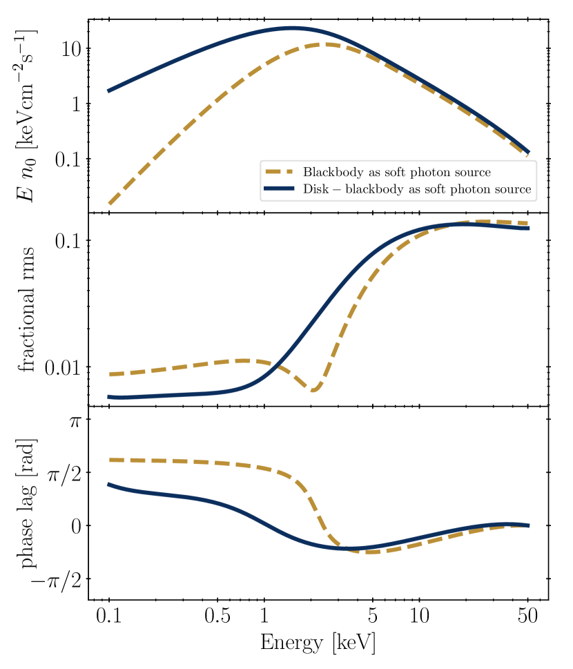
Figure 1: Top panel: The steady-state (i.e. time-averaged) spectra obtained from the solution using either a bbody (olive) or a diskbb (blue) source of seed-soft photons. In the middle and lower panels we plot the energy dependent fractional rms amplitude and phase lag for each seed photon model (the colour convention is the same as in the top panel). In both cases we considered the following parameter values: $\eta=0.5$, $kT_{s}=0.5$ keV, $kT_{e}=20$ keV, $\Gamma=3.5$

In the following figures we present the fractional rms and phase lags obtained with our model, using a diskbb spectrum as the source of soft photons. We do so by independently varying each of the input parameters of the model. In all these figures, we use the same spectrum of Fig. 1 as a guideline, which we plot with a solid black line.

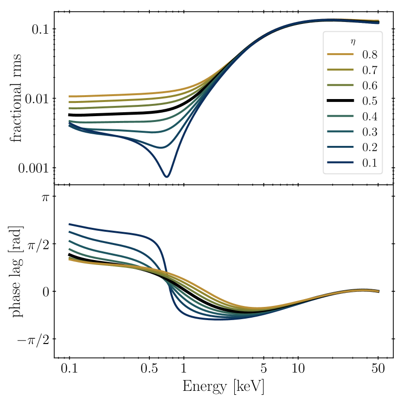
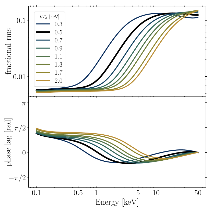
Figure 2: Plot of the energy dependent fractional rms and lags considering a disk-blackbody as soft photon source for different parameter values. On the left panel we show the behaviour of both spectra for different feedback values, from 0.1 (blue) to 0.8 (olive), leaving the other parameters fixed on $kT_{s}=0.5$ keV, $kT_{e}=20$ keV, $\Gamma=3.5$. On the right panel we fix the feedback to $\eta=0.5$ and we varied $kT_{s}$ to explore the spectra for different values of the soft photon source temperature, from 0.3 keV (blue) to 2.0 keV (olive). In both panels we display in black the same fractional rms and lag spectra as in Fig. 1, using $\eta=0.5$, $kT_{s}=0.5$ keV, $kT_{e}=20$ keV, $\Gamma=3.5$ for a disk-blackbody case.

3.1 The feedback fraction and the soft-photon source

On the left panel of Fig. 2 we present the rms and lag spectra for different values of the feedback fraction parameter, $\eta$, ranging from very-low feedback, 0.1 in blue, to very-high feedback, 0.8 in olive. For this configuration, at high energies ($E\gtrsim 5$ keV) the model predicts that both the rms and lags are independent of the feedback fraction, showing essentially identical curves for both the rms and lags. This independence arises as feedback photons are re-emitted following the spectrum of the soft photon source, which dominates below 2 keV but is negligible above 5 keV. At low energies ($E\la 5$ keV) the curves start to separate according to the feedback fraction. For $\eta\gtrsim 0.4$, the rms amplitudes flatten to values of $\sim$1% below 1 keV, while for $\eta<0.4$ the rms decreases further around 0.8 keV, revealing a pivot point for the lowest values of the feedback fraction, and increases again to $\sim$0.5–0.8% at 0.1 keV. At the same time, the lags have a minimum in the 1–5 keV energy range, with the energy of the minimum decreasing as the feedback fraction decreases. For energies below the pivot point ($E<1$ keV), the lags increase again being sharper for the lowest feedback, as in the bbody case (García et al., in prep.).

On the right panel of Fig. 2 we display the behaviour of the variability spectra for different values of the soft photon source temperature, $kT_{s}$, ranging from 0.4 keV in blue to 2 keV in olive. This figure shows that the model predicts essentially the same rms curves for all values of $kT_{s}$ but shifted to higher energies as the soft-photon temperature increases. For $kT_{\rm s}=0.3$ keV the rise of the rms amplitude takes place at 0.4 keV and it moves to the right as $kT_{\rm s}$ increases, reaching $\sim$3 keV for a temperature of 2.0 keV. Similarly, the energy of the minimum in the lags is higher for higher values of $kT_{s}$, going from $\sim$2 keV for $kT_{\rm s}=0.3$ keV to $\sim$14 keV for $kT_{\rm s}=2.0$ keV, suggesting a correlation between both quantities. We fitted the relation between $kT_{\rm s}$ and the energy of the minimum in the lag spectrum, $E_{\rm min}$, with a linear function and found a very significant correlation (correlation coefficient $r=0.999$, with a probability of $10^{-32}$ for the hypothesis that the data are not correlated), $E_{min}\approx 6.87kT_{s}$ in keV.

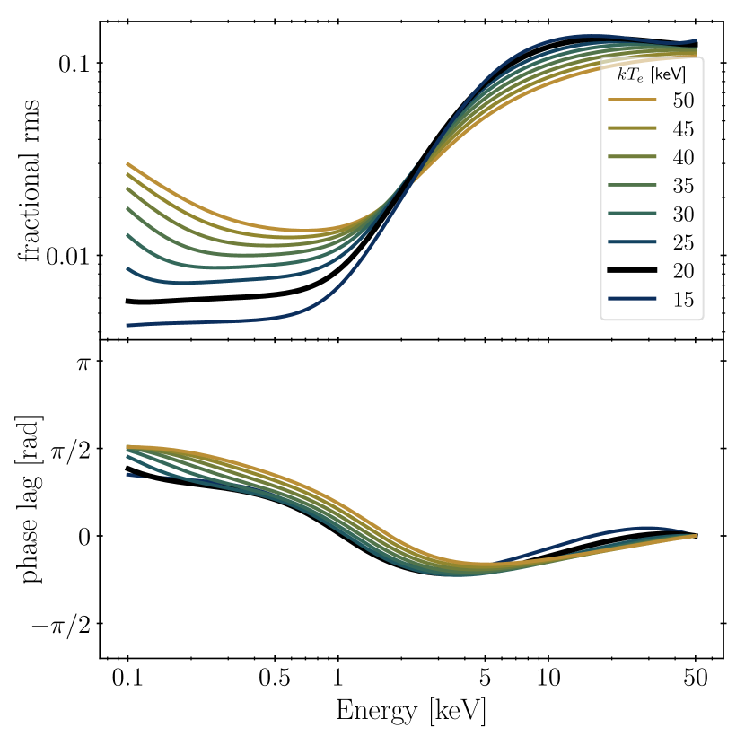
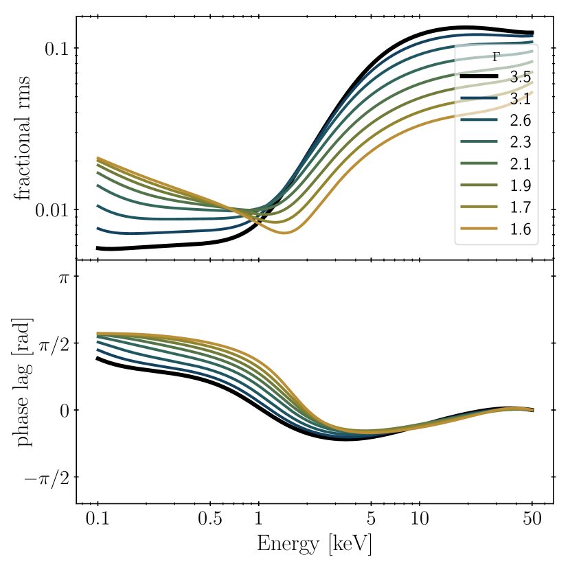
Figure 3: Same plot as Fig. 2 but here we explore the behaviour of the spectra varying independently the corona temperature and the photon index. On the left panel we consider $\eta=0.5$, $kT_{s}=0.5$ keV, $\Gamma=3.5$ and $kT_{e}$ assuming values from 15 keV (blue) to 50 keV (olive). On the right panel we fix $kT_{e}=20$ keV and we vary the photon index from 1.6 (olive) to 3.5 (blue). The black lines are the same as in Fig. 2

3.2 The effect of the corona parameters

On the left panel of Fig. 3 we show the rms and lag spectra as a function of the corona temperature, $kT_{e}$, for values from 15 keV (in blue) to 50 keV (in olive). Overall, the rms amplitude increases with energy from $\sim$1% to $\sim$10% becoming roughly flat above $\sim$10 keV. We see that at energies higher than $\gtrsim$2 keV, though very similar, the model predicts larger rms amplitudes for lower $kT_{\rm e}$ values. Around 2 keV all curves come together and as the energy decreases below $E\la 2$ keV, the trend of the rms amplitude with $kT_{\rm e}$ changes such that that the rms amplitude increases as $kT_{\rm e}$ increases. The lag spectra are smoother at high than at low values of $kT_{e}$. For energies below $\sim$3–5 keV the lags are soft, as they decrease with energy mainly due to feedback. For energies above $\sim$3–5 keV the lags become hard due to Comptonisation. For energies $E>kT_{e}$, the lags reach a local maximum and become soft again, due to Compton down-scattering.

The right panel of Fig. 3 corresponds to different values of the photon index, $\Gamma$. As the electron temperature is fixed for every curve at $kT_{e}=20$ keV, changes in the photon index reflect changes in the optical depth, $\tau$, following this relation: $\Gamma=\sqrt{\frac{9}{4}+\frac{1}{\frac{kT_{e}}{511~{}\mathrm{keV}}\tau(1+\tau/3)}}~{}-~{}\frac{1}{2}$. We considered values of $\Gamma$ ranging from 1.6 in olive (which correspond to $\tau=4.64$) to 3.5 in blue ($\tau=1.3$). At energies below 1 keV, the model predicts higher rms amplitudes for lower $\Gamma$ values. In the 1–2 keV energy range a pivot point shows up for $\Gamma\lesssim 2.6$, and it becomes deeper as $\Gamma$ decreases. Meanwhile, above $\sim$2 keV the rms amplitudes are larger for higher values of $\Gamma$. For photons with energies below 4 keV the model yields softer lags for smaller photon indices. Concomitantly with the appearance of the pivot point in the rms, the fall in the lags becomes steeper for lower $\Gamma$, as the pivot point becomes deeper in the rms spectrum. Around 4 keV the curves start to overlap until it becomes difficult to separate one from the other for energies $\gtrsim$5 keV.

3.3 Model application to MAXI J1348–630

MAXI J1348–630 is a BH LMXB discovered in outburst on 2019 January 26 with the MAXI instrument on board the ISS (Yatabe et al., 2019; Tominaga et al., 2020). The source showed a transition from the low-hard to the high-soft state, first detected with MAXI and later confirmed with INTEGRAL (Cangemi et al., 2019), followed by a strong radio flare (Carotenuto et al., 2019, 2022). Across the outburst, a thorough follow-up was performed with the NICER instrument in the 0.2–12 keV energy range (Gendreau et al., 2012), and the spectral-timing analysis of a prominent type-B QPO observed during this transitions was presented in detail by Belloni et al. (2020). In their Figure 4, Belloni et al. (2020) show the energy-dependent fractional-rms amplitude and phase lags of the type-B QPO in MAXI J1348–630. The strong QPO was detected in the full energy range, from 0.75 to 10 keV, at a stable QPO frequency $\nu_{0}\approx 4.45$ Hz, with fractional rms amplitudes increasing from $\la$1% at the lowest energies to $\sim$10% at the highest ones. In addition, the lag-energy spectrum shows that photons with energies both below and above those in the 2–2.5 keV, the reference band, lag behind the photons in the reference band with an average delay of $\sim$32 ms for photons with energies below the reference band, and $\sim$21 ms for photons above that.

García et al. (2021) applied the model originally developed by Karpouzas et al. (2020), including a black-body source of soft photons, and found a relatively good fit to the lag spectrum, but failed to explain the high fractional rms values observed at high energies. They then introduced two independent, but physically coupled, Comptonisation regions, with which they achieved good fits to both the rms and lag spectra of the QPO. These two regions, which they called small and large. have sizes of $\sim$30 and $\sim$700 $R_{g}$, where $R_{g}$ is the gravitational radius assuming a 10 M_⊙ BH, with feedback fractions of $\sim$20 and $\sim$0.8%, respectively. They also found a soft-photon source temperature of $kT_{\rm bb}\sim 0.35$ keV, lower than the temperature of the diskbb component from the best-fit to the time-averaged spectrum ($\sim$0.6 keV, Belloni et al., 2020); as explained by García et al. (2021), this is a consequence of the spectral differences between a diskbb and a bbody.

Given the use of a diskbb component in the model described here, we tried and fitted the diskbb variant of our variable-Comptonisation spectral-timing model, that we so-called vkompthdk, to the same dataset.

3.3.1 Single-component Comptonisation model vkompthdk

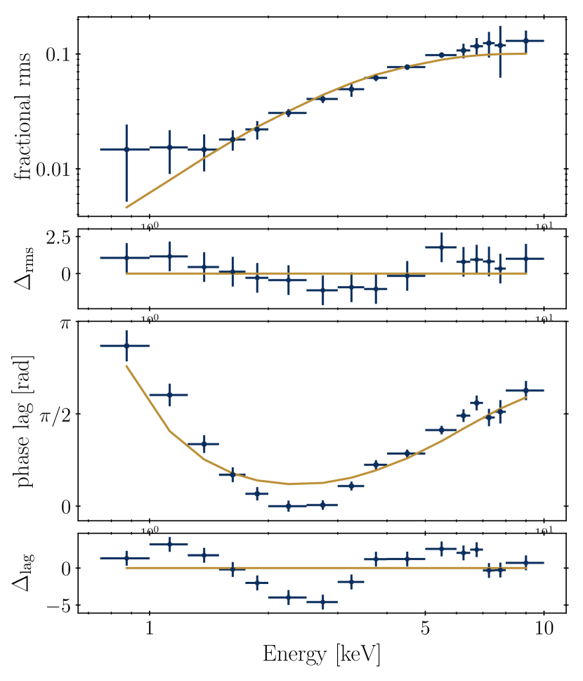
Figure 4: Fractional rms (upper panels) and phase-lag spectra (lower panels) of the 4.45 Hz type-B QPO of MAXI J1348–630. The solid lines represent the best-fitting vkompthdk model obtained for a corona size of $\sim$11 000 km and a $\sim$35% feedback fraction for a diskbb soft-photon source with a temperature of $\sim$0.45 keV. Residuals, $\Delta$ = (data–model)/error, are also shown. The error bars of the rms amplitude were multiplied by a factor of five and rms dilution has been included (see text for details).

Table 1: Best-fitting values of the physical parameters of MAXI J1348–630 and their corresponding 1-$\sigma$ (68%) uncertainties obtained with a single-component vkompthdk model.

$kT_{e}$	$\Gamma$	$\tau$	$kT_{s}$	$L$	$\eta$	${\delta H}_{\rm ext}$	$\chi_{\nu}^{2}$ (dof)
(keV)			(keV)	($10^{3}$ km)		(%)
20†	3.5†	1.3†	0.44$\pm$0.02	11$\pm$1	0.37$\pm$0.06	13$\pm$1	3.45 (27 dof)

In order to fit the fractional rms and phase lags of the type-B QPO of MAXI J1348–630 using the vkompth model introduced in this work, we used XSPEC v12.12.0g (Arnaud, 1996). For this, we compiled the vkompth model written in Fortran against the XSPEC libraries and loaded it as an external model; we also wrote the rms and phase lag spectra in PHA format and created the corresponding response (RMF) files. The best-fitting model was obtained using the Levenberg-Marquardt algorithm and uncertainties in the parameters were calculated by running Markov Chain Monte Carlo (MCMC) simulations of $10^{5}$ samples from 60 walkers, using the Goodman-Weare algorithm provided by XSPEC.

Along this process we kept the corona temperature, $kT_{e}$ fixed to 20 keV and the power-law index, $\Gamma$ to 3.5 (Belloni et al., 2020), which yields an optical depth of $\sim$1.3. The rest of the physical parameters were left free to vary. As in García et al. (2021), while fitting the one-component vkompthdk model, we increased the errors in the fractional rms amplitudes by a factor of five to match the uncertainties in the lags.

As our model only considers variations in the Comptonisation component, nthcomp, whereas the best-fitting model to the time-average spectrum found by Belloni et al. (2020) was diskbb+nthcomp+gaussian, we introduced a correction to the fractional rms amplitude computed in the model to take into account the fraction of photons that are emitted by the accretion disk component diskbb and the Fe-line gaussian, and reach the observer without being Comptonised. This correction takes into account that, compared to the prediction of vkompthdk, the observed fractional rms amplitudes are diluted by a factor ${\tt nthcomp}/{({\tt nthcomp+diskbb+gaussian})}$.

In Figure 4 we present the best-fitting model and residuals obtained with a single-Comptonisation region. The corresponding best-fitting parameters and their 1-$\sigma$ (68%) uncertainties are summarized in Table LABEL:tab:vkompthdk. Corner plots associated to the MCMC chains can be found in Appendix A. Similar to what was found by García et al. (2021) using vkompthbb, with a bbody as the source of soft-photons, the vkompthdk model reproduces the trends of both the fractional rms amplitude and phase lags, but the fit is far from being statistically acceptable, with $\chi_{\nu}^{2}=3.45$ for 27 d.o.f. Using the vkompthdk model, the fit improves, yielding a higher fractional rms variability amplitudes than the vkompthbb model above $\sim$5 keV, as shown by the data, but fails to reproduce the lag spectrum at mid-energies ($2-3$ keV). The best-fitting model requires a relatively large corona of 11 000 km ($\sim$600 $R_{g}$, for a 10 M_⊙ BH), with a relatively low feedback fraction of $\sim$35%. The diskbb temperature is $\sim$0.45 keV, higher than the value found by García et al. (2021) for a bbody spectrum ($\sim$0.2 keV), but much more compatible with the best-fitting $kT_{\rm dbb}$ obtained by Belloni et al. (2020) and Zhang et al. (2021) for the time-averaged spectra of the source, $kT_{s}\sim$0.6 keV. This result makes the model clearly more self-consistent in terms of the observed time-average and variable energy-dependent spectra. Finally, the amplitude of the oscillation of the external heating source is $\sim$13%, higher than the value found by García et al. (2021) for the fit with vkompthbb ($\sim$4%).

3.3.2 Two-component Comptonisation model vkdualdk

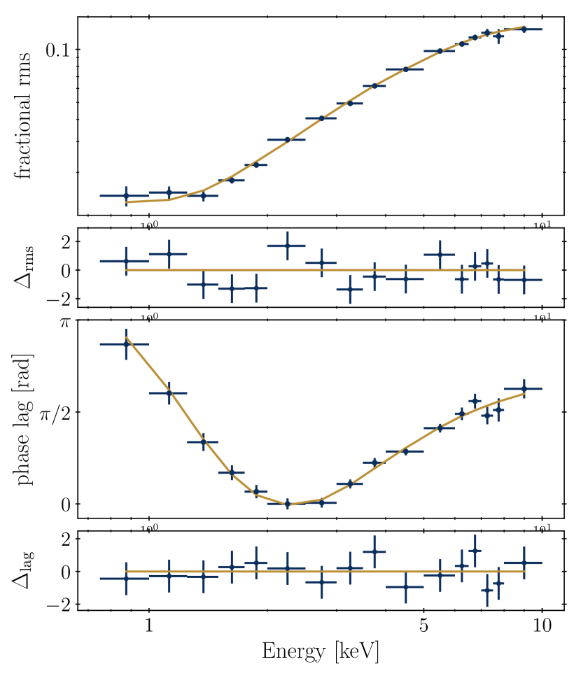
Figure 5: Energy-dependent fractional rms amplitude (upper panels) and phase lags (lower panels) of the 4.45 Hz type-B QPO of MAXI J1348–630. The best-fitting models (solid lines) are obtained using a combination of two Comptonisation components (vkdualdk model). Residuals, $\Delta$ = (data–model)/error, are also shown. Dilution of the rms by the disk component has been included (see text for details).

Table 2: Same as Table LABEL:tab:vkompthdk for the two-component vkdualdk model.

$kT_{e}$	$\Gamma$	$\tau$	$kT_{s,1}$	$kT_{s,2}$	$L_{1}$	$L_{2}$	$\eta_{1}$	$\eta_{2}$	${\delta H}_{{\rm ext},1}$	${\delta H}_{{\rm ext},2}$	$\phi$	$\chi_{\nu}^{2}$ (dof)
(keV)			(keV)	(keV)	($10^{3}$ km)	($10^{3}$ km)			(%)	(%)	(rad)
20†	3.5†	1.3†	0.93$\pm$0.11	0.42$\pm$0.02	0.16$\pm$0.06	13.4${}^{+3.6}_{-2.3}$	>0.88	0.27$\pm$0.10	25$\pm$6	20$\pm$3	3.0$\pm$0.1	0.96 (22 dof)

Following García et al. (2021), and given the large $\chi^{2}$ obtained using the single-component Comptonisation model vkompthdk, we also explored the possibility that the variability spectra arises from two Comptonisation regions that we also call small (1) and large (2); we call this dual model vkdualdk . For this, in order to match the properties of the time-averaged spectrum, we consider that both regions have $kT_{e,1-2}=20$ keV and $\Gamma_{1-2}=3.5$ (see Belloni et al., 2020; Zhang et al., 2021). While fitting the QPO data with this vkdualdk model, we consider the actual 1-$\sigma$ errors of both rms and phase lags and take into account the rms dilution introduced in the previous sub-section.

In Figure 5 we show the best-fits and residuals found using the vkdualdk model. The corresponding best-fitting parameters and their 1-$\sigma$ (68%) uncertainties are presented in Table LABEL:tab:vkdualdk, where subindices 1 and 2 correspond to the small and large corona components, respectively. In Appendix A we present the corner plot obtained from the MCMC chain for the most relevant physical parameters of this model.

The best-fitting vkdualdk model matches the data statistically very well, with $\chi_{\nu}^{2}=0.96$ for 22 d.o.f, significantly better than the fit with single-component model. The dual model is able to explain simultaneously both the rms amplitudes leveling below $\sim$1.5 keV and the steady increase up to $\gtrsim$10% at $\sim$5-10 keV, while showing the same overall trend of the $U$-shaped lag spectrum which also levels off in that same energy range. The residuals, on the other hand, show no systematic trends. The best-fitting model yields a small Comptonisation region of $\sim$150 km ($\sim$8 $R_{g}$ for a 10 M_⊙ BH) with very high feedback (>90%) and a rather high seed temperature of $\sim$0.9 keV, pointing to the innermost parts of the diskbb component as the source of soft-photons, plus a large Comptonisation region of $\sim$12 200 km ($\sim$650 $R_{g}$) with relatively low feedback fraction of $\sim$25%, and a diskbb temperature of $\sim$0.4 keV, similar to the Comptonisation region found with the vkompthdk model presented in the previous sub-section. The oscillations of the two components have a lag, $\phi\sim$3.0$\pm$0.1 rad. The amplitude of the oscillation of the external-heating source are roughly $\sim$23% and $\sim$20%, respectively.

3.4 Application to type-C QPOs in GRS 1915+105

To verify whether this version of the model is also applicable to type-C QPOs in BH X-ray binaries, we fitted the vkompthdk model to the rms and lag spectra of the type-C QPO in the BH candidate GRS 1915+105 (Zhang et al., 2020; Méndez et al., 2022). This type-C QPO was originally fitted using the vkompthbb model in 398 RXTE observations (García et al., 2022). In their Figures 4, 5 and 6 García et al. (2022) presented the best-fitting values of, respectively, the feedback fraction, $\eta$, the corona size, $L$, and the blackbody temperature, $kT_{s}$, as a function of the QPO frequency, $\nu_{0}$. Both $\eta$ and $kT_{s}$ show increasing trends with $\nu_{0}$, and two families of points are apparent in the plots: for $\nu_{0}\lesssim 1.8$ Hz, the source shows low feedback fraction ($\eta\lesssim 0.3$) and low temperature ($kT_{s}\lesssim 0.2$ keV), whereas when $\nu_{0}\gtrsim 2.5$ Hz the feedback becomes rather large ($\eta\gtrsim 0.8$) and the black-body temperature increases to $0.7-2$ keV. Meanwhile, in the intermediate $1.8-2.5$ Hz range, both families coexist. On the other hand, the corona size rapidly decreases from $\gtrsim$10⁴ km to $\sim$10² km as $\nu_{0}$ increases from 0.5 to 2 Hz, and slowly increases again reaching intermediate sizes of $\sim$10³ km when $\nu_{0}\approx 4-6$ Hz . They also showed that, at the same QPO frequency, higher corona temperatures correspond to larger corona sizes.

When using the vkompthdk model presented in this work to fit this same QPO dataset, despite small differences in the individual values in each particular fit, for every relevant parameter we found consistent trends with those found in the earlier work from García et al. (2022) using vkompthbb that were described above. This was somehow expected since, as we showed at the beginning of this Section, the differences between the vkompthbb and vkompthdk models become significant below $\sim$2 keV, while RXTE is only sensitive above 3 keV.

4 Discussion

We developed a new version of the time-dependent Comptonization model of Karpouzas et al. (2020) in which we use an accretion disc instead of a blackbody as the source of seed photons that are subsequently inverse-Compton scattered in a corona. The new model can be used to fit the rms amplitude and phase lag spectra of low-frequency QPOs in BH-LMXBs. We also implemented a logarithmic grid to solve the time-dependent Kompaneets equation that describes the variability of the disk/corona system, which accelerates the code by two orders of magnitude compared to the version in Karpouzas et al. (2020).

The fractional rms variability of the LFQPOs in BH LMXBs increases with energy, from $\mathbin{\lower 3.0pt\hbox{$\hbox to0.0pt{\raise 5.0pt\hbox{$\char 60\relax$}\hss}\mathchar 29208\relax$}}$1% at energies below 1-2 keV (Belloni et al., 2020) to 10-20% at $\sim$30-50 keV (Zhang et al., 2017; Zhang et al., 2020), and in some cases even up-to 100-200 keV (e.g., Huang et al., 2018; Ma et al., 2021). At those energies, Comptonisation dominates the time-averaged spectrum and hence this process must be the mechanism responsible for the radiative properties of these QPOs. In our model, the QPO is a small oscillation of the source spectrum around the time-averaged spectrum, caused by fluctuations of the thermodynamic properties of either the Comptonising medium or the accretion disk.

The model was originally developed for the high-frequency QPOs in NS-LMXBs considering a bbody spectrum, representing the surface of the NS itself or the boundary layer, as the source of soft-photons for Comptonisation (Lee & Miller, 1998; Lee et al., 2001; Kumar & Misra, 2014; Karpouzas et al., 2020). The same model was later applied to model low-frequency QPOs in BH candidates (García et al., 2021; Karpouzas et al., 2021), who considered the same kind of soft-photon source. In this work we modified the model to have a disk-blackbody (diskbb) as the source of soft-photons; the disc photons are injected into a spherical corona of homogeneously distributed hot electrons. The soft photons are inverse-Compton scattered by these electrons, and escape the corona with, on average, a higher energy than the one they had when they entered the corona. Because the photons that suffer more scatterings escape the corona at a later time, and with higher energies than those photons that escape directly or suffer less scatterings, the hard photons lag the soft ones (introducing hard lags). If a fraction of the up-scattered photons returns to the disc and is reprocessed and thermalised, a process that we call feedback, low-energy photons will escape the corona after the hard photons leading to soft lags.

We note that our model is based upon two assumptions: (i) The soft-photon source (a disk blackbody in this paper or a blackbody in Karpouzas et al., 2020) is spherically symmetric and the seed photons are emitted isotropically in the corona (Sunyaev & Titarchuk, 1980; Zdziarski et al., 1996; Życki et al., 1999) (ii) The corona is spherically symmetric and homogeneous, and its optical depth, and therefore its density, remain constant during the oscillation. In the future we hope to generalize some of these hypotheses however, at this stage, these are necessary assumptions to be able to solve the mathematics involved in the problem in a semi-analytic way.

We found that when the soft-photon source is modelled as a diskbb the fractional rms amplitude and phase lag spectra of the QPO have a smoother behaviour than when one uses a blackbody soft-photon source. In general, at high energies there is no significant difference in the rms and lag spectra between the diskbb and blackbody cases, consistent with the fact that both time-averaged spectra, nthcomp and bbody, are almost identical at high energies. We also analyzed the dependence of both the rms amplitude and phase lags of the QPO upon the different physical parameters of the model. At energies above 1 keV, the rms amplitude depends upon the temperature of both the corona and the soft photon source, but primarily on the optical depth of the corona (Fig. 3), whereas the feedback fraction $\eta$ does not modify the rms spectrum. Instead, at energies below 1 keV, the rms amplitudes are affected by all parameters except for the soft-photon source temperature. The slope of the phase-lag spectrum, on the other hand, depends strongly on $\eta$. For a very low value of $\eta$ the lags are hard, while as $\eta$ increases the lags soften (see left panel of Fig. 2). While at energies above $\sim$5 keV the lag spectra are essentially independent of the parameter values, at energies below $\sim$5 keV the shape of the lag spectra changes significantly when the parameters change. For instance, the lags become softer with increasing corona temperature, $kT_{e}$, or with decreasing photon index, $\Gamma$, or feedback fraction, $\eta$. Finally, we found a strong correlation between the minimum in the phase lag spectrum, the increasing energy in the rms, and the soft-photon source temperature, $kT_{s}$, which is apparent on the right panel of Fig. 2.

Our optimization of the numerical code, which now uses a logarithmic energy grid, makes it fast enough such that it is computationally possible to use our vkompth model as a local model of XSPEC to fit the time-dependent as well as the time-averaged spectra in the standard way. As an example of the application of the model to a low-frequency QPO in a BH LMXB, we have chosen to fit the available data from the type-B in MAXI J1348–630 obtained while the source was transitioning from the high to the soft states (Belloni et al., 2020). This dataset was early fitted using our model with a bbody soft-photon source by García et al. (2021). The available data comprises the energy-dependent fractional rms and phase lags associated to this QPO with a $\nu_{0}=4.55$ Hz. When comparing those fits obtained using a diskbb model to those from García et al. (2021) based on a bbody source of soft-photons, we found that the former are statistically better, and that the physical parameters retrieved are more appropriate when compared both to those derived from the steady-state or time-averaged spectra, and to the overall scenario.

Following García et al. (2021), we initially fitted simultaneously the rms and lag spectra of this QPO with the single-Comptonisation region model, vkompthdk in XSPEC. The best-fitting model reproduces the trends in the data quite well, but the fit is statistically unacceptable, with a high reduced $\chi_{\nu}^{2}=3.45$. The fit requires a large corona, $L\sim 600~{}R_{g}$, with relatively low feedback, $\eta\sim 35$%. While this may appear to be too large a corona, we note that such a large corona ($L\sim 100-500~{}R_{g}$) was also found in MAXI J1820+70 during the transition from the high to the soft state, from fits to the broadband lags using a lamp-post reverberation model (Wang et al., 2021), and a large corona, $L\sim$100 $R_{g}$, was also inferred in the case of Cyg X-1 using polarimetric measurements from PoGO+ (Chauvin et al., 2018). We also fitted a model with two-Comptonisation regions, which we call vkdualdk, to the same data. We found that the best-fitting model requires a large corona with similar characteristics to those found using the vkompthdk model, and a small corona of $L\sim$150 km ($\sim$8 $R_{g}$ for a 10 M_⊙ BH) with a very high feedback fraction, $\eta>$90%. We interpret this solution as a dual corona formed by a compact and hot region situated very close to the BH and fed by the innermost parts of the accretion disk with a relatively high effective temperature, $kT_{s}\sim 0.9$ keV, and a large and extended region fed by a more external part of the accretion disk, and thus having a lower effective temperature, $kT_{s}\sim$0.4 keV); this large region may be associated to the base of the extended jet which starts to develop during the state transition in MAXI J1348–630 (Carotenuto et al., 2022).

We also fitted the vkompthdk model presented here to 398 RXTE observations of GRS 1915+105 containing a type-C QPO. For every relevant physical parameter of the model, we found consistent trends with QPO frequency to those obtained using a black body, vkompthbb, as the soft-photon source (see Figures 4, 5 and 6 in García et al., 2022). This was expected given the energy coverage from RXTE, which was not sensitive below $\sim$3 keV. In addition, recently Zhang et al. (2022) successfully applied the vkompthdk model to fit the type-C QPOs in MAXI J1535–571, using HXMT data ranging from 1 to 100 keV. Therefore, we conclude that this variable-Comptonisation model is able to explain both type-B and type-C low-frequency QPOs in BH LMXB binaries.

Data Availability

The model developed in this paper is available through https://github.com/candebellavita/vkompth. We encourage people interested in applying the model to data to contact the authors for further support.

Appendix A MCMC corner plots

As explained in Sec. 3, we fitted the vkompth model using XSPEC (Arnaud, 1996) using the Levenberg-Marquardt algorithm. After finding the appropriate minimum, in order to estimate the uncertainties in the physical parameters provided by the models, we ran MCMC chains of $10^{5}$ steps using 60 walkers under the Goodman-Weare scheme in XSPEC. We then used the tkXspecCorner program to interactively create corner plots of the main physical parameters that we present on Figures 6 and 7 for the vkompthdk and the vkdualdk models, respectively. As usual, in the lower-left panels of the corner plots we show the joint-probabilities of each pair of relevant physical parameters of the models, while in the diagonal we show the individual probability of each parameter, including both the median and 68% confidence intervals in the top labels.

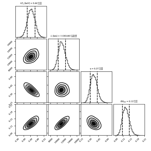
Figure 6: Corner plot of the physical parameters of MAXI J1348–630  obtained with the single Comptonisation model vkompthdk introduced in this paper, which includes a diskbb soft-photon source characterised by its temperature, $kT_{s}$. The parameters of the corona include its physical size, $L$, the feedback fraction, $\eta$, and the amplitude of the external heating rate oscillation, $\delta H_{\rm ext}$. Median and 68% credible-interval for each parameter are indicated at the top of each diagonal panel.

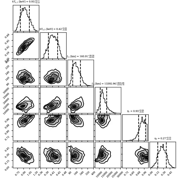
Figure 7: Same as Figure 6 but for the main best-fitting parameters obtained using a two-component dual model, named vkdualdk.

References

- Arnaud (1996) Arnaud K. A., 1996, in Jacoby G. H., Barnes J., eds, Astronomical Society of the Pacific Conference Series Vol. 101, Astronomical Data Analysis Software and Systems V. p. 17
- Belloni & Altamirano (2013) Belloni T. M., Altamirano D., 2013, MNRAS, 432, 10
- Belloni & Motta (2016) Belloni T. M., Motta S. E., 2016, in Bambi C., ed., Astrophysics and Space Science Library Vol. 440, Astrophysics of Black Holes: From Fundamental Aspects to Latest Developments. p. 61 (arXiv:1603.07872), doi:10.1007/978-3-662-52859-4_2
- Belloni et al. (2005) Belloni T., Homan J., Casella P., van der Klis M., Nespoli E., Lewin W. H. G., Miller J. M., Méndez M., 2005, A&A, 440, 207
- Belloni et al. (2020) Belloni T. M., Zhang L., Kylafis N. D., Reig P., Altamirano D., 2020, MNRAS, 496, 4366
- Berger et al. (1996) Berger M., et al., 1996, ApJ, 469, L13
- Cangemi et al. (2019) Cangemi F., Belloni T., Rodriguez J., 2019, The Astronomer’s Telegram, 12471, 1
- Carotenuto et al. (2019) Carotenuto F., Tremou E., Corbel S., Fender R., Woudt P., Miller-Jones J., 2019, The Astronomer’s Telegram, 12497, 1
- Carotenuto et al. (2022) Carotenuto F., Tetarenko A. J., Corbel S., 2022, arXiv e-prints, p. arXiv:2202.01514
- Casella et al. (2005) Casella P., Belloni T., Stella L., 2005, ApJ, 629, 403
- Chauvin et al. (2018) Chauvin M., et al., 2018, Nature Astronomy, 2, 652
- Fabian et al. (1989) Fabian A. C., Rees M. J., Stella L., White N. E., 1989, MNRAS, 238, 729
- García et al. (2021) García F., Méndez M., Karpouzas K., Belloni T., Zhang L., Altamirano D., 2021, MNRAS, 501, 3173
- García et al. (2022) García F., Karpouzas K., Méndez M., Zhang L., Zhang Y., Belloni T., Altamirano D., 2022, MNRAS, in press.
- Gendreau et al. (2012) Gendreau K. C., Arzoumanian Z., Okajima T., 2012, in Space Telescopes and Instrumentation 2012: Ultraviolet to Gamma Ray. p. 844313, doi:10.1117/12.926396
- Giannios et al. (2004) Giannios D., Kylafis N. D., Psaltis D., 2004, A&A, 425, 163
- Gilfanov et al. (2003) Gilfanov M., Revnivtsev M., Molkov S., 2003, A&A, 410, 217
- Homan et al. (2001) Homan J., Wijnands R., van der Klis M., Belloni T., van Paradijs J., Klein-Wolt M., Fender R., Méndez M., 2001, ApJS, 132, 377
- Huang et al. (2018) Huang Y., et al., 2018, ApJ, 866, 122
- Ingram & Motta (2020) Ingram A., Motta S., 2020, arXiv e-prints, p. arXiv:2001.08758
- Ingram et al. (2009) Ingram A., Done C., Fragile P. C., 2009, MNRAS, 397, L101
- Kara et al. (2019) Kara E., et al., 2019, Nature, 565, 198
- Karpouzas et al. (2020) Karpouzas K., Méndez M., Ribeiro E. M., Altamirano D., Blaes O., García F., 2020, MNRAS, 492, 1399
- Karpouzas et al. (2021) Karpouzas K., Méndez M., García F., Zhang L., Altamirano D., Belloni T., Zhang Y., 2021, MNRAS, 503, 5522
- Kazanas et al. (1997) Kazanas D., Hua X.-M., Titarchuk L., 1997, ApJ, 480, 735
- Kompaneets (1957) Kompaneets A. S., 1957, Soviet Journal of Experimental and Theoretical Physics, 4, 730
- Kumar & Misra (2014) Kumar N., Misra R., 2014, MNRAS, 445, 2818
- Lee & Miller (1998) Lee H. C., Miller G. S., 1998, MNRAS, 299, 479
- Lee et al. (2001) Lee H. C., Misra R., Taam R. E., 2001, ApJ, 549, L229
- Lightman & Zdziarski (1987) Lightman A. P., Zdziarski A. A., 1987, ApJ, 319, 643
- Ma et al. (2020) Ma X., et al., 2020, Nature Astronomy,
- Ma et al. (2021) Ma X., et al., 2021, Nature Astronomy, 5, 94
- Markoff et al. (2005) Markoff S., Nowak M. A., Wilms J., 2005, ApJ, 635, 1203
- Mastroserio et al. (2019) Mastroserio G., Ingram A., van der Klis M., 2019, MNRAS, 488, 348
- Méndez & Belloni (2021) Méndez M., Belloni T. M., 2021, in Belloni T. M., Méndez M., Zhang C., eds, Astrophysics and Space Science Library Vol. 461, Astrophysics and Space Science Library. pp 263–331 (arXiv:2010.08291), doi:10.1007/978-3-662-62110-3_6
- Méndez & van der Klis (1997) Méndez M., van der Klis M., 1997, ApJ, 479, 926
- Méndez et al. (2001) Méndez M., van der Klis M., Ford E. C., 2001, ApJ, 561, 1016
- Méndez et al. (2022) Méndez M., Karpouzas K., García F., Zhang L., Zhang Y., Belloni T., Altamirano D., 2022, Nature Astronomy, in press
- Mitsuda et al. (1984) Mitsuda K., et al., 1984, PASJ, 36, 741
- Miyamoto et al. (1988) Miyamoto S., Kitamoto S., Mitsuda K., Dotani T., 1988, Nature, 336, 450
- Morgan et al. (1997) Morgan E. H., Remillard R. A., Greiner J., 1997, ApJ, 482, 993
- Reig & Kylafis (2021) Reig P., Kylafis N. D., 2021, A&A, 646, A112
- Rodriguez et al. (2002) Rodriguez J., Durouchoux P., Mirabel I. F., Ueda Y., Tagger M., Yamaoka K., 2002, A&A, 386, 271
- Shakura & Sunyaev (1973) Shakura N. I., Sunyaev R. A., 1973, A&A, 500, 33
- Sobolewska & Życki (2006) Sobolewska M. A., Życki P. T., 2006, MNRAS, 370, 405
- Stella & Vietri (1998) Stella L., Vietri M., 1998, ApJ, 492, L59
- Sunyaev & Titarchuk (1980) Sunyaev R. A., Titarchuk L. G., 1980, A&A, 500, 167
- Sunyaev & Truemper (1979) Sunyaev R. A., Truemper J., 1979, Nature, 279, 506
- Tominaga et al. (2020) Tominaga M., et al., 2020, ApJ, 899, L20
- Wang et al. (2021) Wang J., et al., 2021, ApJ, 910, L3
- Yadav et al. (2016) Yadav J. S., et al., 2016, ApJ, 833, 27
- Yatabe et al. (2019) Yatabe F., et al., 2019, The Astronomer’s Telegram, 12425, 1
- Zdziarski et al. (1996) Zdziarski A. A., Johnson W. N., Magdziarz P., 1996, MNRAS, 283, 193
- Zhang et al. (2017) Zhang L., Wang Y., Méndez M., Chen L., Qu J., Altamirano D., Belloni T., 2017, ApJ, 845, 143
- Zhang et al. (2020) Zhang L., et al., 2020, MNRAS, 494, 1375
- Zhang et al. (2021) Zhang L., et al., 2021, MNRAS, 505, 3823
- Zhang et al. (2022) Zhang Y., et al., 2022, MNRAS, 512, 2686
- Życki et al. (1999) Życki P. T., Done C., Smith D. A., 1999, MNRAS, 309, 561
- van der Klis (1994) van der Klis M., 1994, ApJS, 92, 511