Reducing Annotation Need in Self-Explanatory Models for Lung Nodule Diagnosis

Abstract

Feature-based self-explanatory methods explain their classification in terms of human-understandable features. In the medical imaging community, this semantic matching of clinical knowledge adds significantly to the trustworthiness of the AI. However, the cost of additional annotation of features remains a pressing issue. We address this problem by proposing cRedAnno, a data-/annotation-efficient self-explanatory approach for lung nodule diagnosis. cRedAnno considerably reduces the annotation need by introducing self-supervised contrastive learning to alleviate the burden of learning most parameters from annotation, replacing end-to-end training with two-stage training. When training with hundreds of nodule samples and only $1\%$ of their annotations, cRedAnno achieves competitive accuracy in predicting malignancy, meanwhile significantly surpassing most previous works in predicting nodule attributes. Visualisation of the learned space further indicates that the correlation between the clustering of malignancy and nodule attributes coincides with clinical knowledge. Our complete code is open-source available: https://github.com/diku-dk/credanno.

1 Introduction

(a) Previous methods

(b) cRedAnno

Figure 1: Concept illustration. (a) Previous works are trained end-to-end, where all parameters are learned from the annotations. (b) Our proposed cRedAnno uses two-stage training, where most of the parameters are learned during the first stage in a self-supervised manner. Therefore, in the second stage, only few annotations are needed to train the predictors.

Lung cancer is one of the leading causes of cancer deaths worldwide due to its high morbidity and low survival rate [9]. In clinical practice, accurate characterisation of pulmonary nodules in CT images is an essential step for effective lung cancer screening [28]. Modern deep-learning-based “black box” algorithms, although achieving accurate classification performance [1], are hardly acceptable in high-stakes medical diagnosis[26].

Amongst recent efforts to develop explainable AI [4] to bridge this gap [24, 26], post-hoc approaches that attempt to explain such “black boxes” are not deemed trustworthy enough [18]. In contrast, feature-based self-explanatory methods are trained to first predict a set of well-known human-interpretable features, and then use these features for the final classification (Fig. 1a)[23, 22, 15]. This is believed to be especially valuable in medical applications because such semantic matching towards clinical knowledge tremendously increases the AI’s trustworthiness [20]. Unfortunately, the required additional annotation on features still limits the applicability of this approach in the medical domain.

This paper aims to minimise additional annotation need for predicting malignancy and nodule attributes in lung CT images. We achieve this by separating the training of model’s parameters into two stages, as shown in Fig. 1b. In Stage 1, the majority of parameters are trained using self-supervised contrastive learning [12, 11, 6] as an encoder to map the input images to a latent space that complies with radiologists’ reasoning for nodule malignancy. In Stage 2, a small random portion of labelled samples is used to train a simple predictor for each nodule attribute. Then the predicted human-interpretable nodule attributes are used jointly with the extracted features to make the final classification.

Our experiments on the publicly available LIDC dataset [2] show that with fewer nodule samples and only $1\%$ of their annotations, the proposed approach achieves comparable or better performance compared with state-of-the-art methods using full annotation [22, 15, 7, 16, 13], and reaches approximately $90\%$ accuracy in predicting all nodule attributes simultaneously. By visualising the learned space, the extracted features are shown to be highly separable and correlated well with clinical knowledge.

2 Method

As the illustrated concept in Fig. 1b, the proposed approach consists of two parts: unsupervised training of the feature encoder and supervised training to predict malignancy with human-interpretable nodule attributes as explanations.

2.0.1 Unsupervised feature extraction

Due to the outstanding results exhibited by DINO [6], we adopt their framework for unsupervised feature extraction, which trains (i) a primary branch $\{E,H\}_{\_}{\theta_{\_}\text{pri}}$, composed by a feature encoder $E$ and a multi-layer perceptron (MLP) prediction head $H$, parameterised by $\theta_{\_}\text{pri}$; (ii) an auxiliary branch $\{E,H\}_{\_}{\theta_{\_}\text{aux}}$, which is of the same architecture as the primary branch, while parameterised by $\theta_{\_}\text{aux}$. After training only the primary encoder $E_{\_}{\theta^{\text{E}}_{\_}\text{pri}}$ is used for feature extraction.

The branches are trained using augmented image patches of different scales to grasp the core feature of a sample. For a given input image $x$, different augmented global views $V^{g}$ and local views $V^{l}$ are generated [5]: $x\rightarrow v\in V^{g}\cup V^{l}$. The primary branch is only applied to the global views $v_{\_}\text{pri}\in V^{g}$, producing $K$ dimensional outputs $z_{\_}\text{pri}=E_{\_}{\theta^{\text{E}}_{\_}\text{pri}}\circ H_{\_}{\theta^{\text{H}}_{\_}\text{pri}}(v_{\_}\text{pri})$; while the auxiliary branch is applied to all views $v_{\_}\text{aux}\in V^{g}\cup V^{l}$, producing outputs $z_{\_}\text{aux}=E_{\_}{\theta^{\text{E}}_{\_}\text{aux}}\circ H_{\_}{\theta^{\text{H}}_{\_}\text{aux}}(v_{\_}\text{aux})$ to predict $z_{\_}\text{pri}$. To compute the loss, the output in each branch is passed through a Softmax function scaled by temperature $\tau_{\_}\text{pri}$ and $\tau_{\_}\text{aux}$: $p_{\_}\text{aux}=\texttt{softmax}(z_{\_}\text{aux}/\tau_{\_}\text{aux})$, $p_{\_}\text{pri}=\texttt{softmax}((z_{\_}\text{pri}-\mu)/\tau_{\_}\text{pri})$, where a bias term $\mu$ is applied to $z_{\_}\text{pri}$ to avoid collapse[6], and updated at the end of each iteration using the exponential moving average (EMA) of the mean value of a batch with batch size $N$ using momentum factor $\lambda\in[0,1)$: $\mu\leftarrow\lambda\mu+(1-\lambda)\frac{1}{N}\sum_{\_}{s=1}^{N}z_{\_}\text{pri}^{(s)}$.

The parameters $\theta_{\_}\text{aux}$ are learned by minimising the cross-entropy loss between the two branches via back-propagation [12]:

$$\theta_{\_}\text{aux}\leftarrow\arg\min_{\_}{\theta_{\_}\text{aux}}\sum_{\_}{v_{\_}\text{pri}\in V^{g}}\sum_{\_}{\begin{subarray}{c}v_{\_}\text{aux}\in V^{g}\cup V^{l}\\ v_{\_}\text{aux}\neq v_{\_}\text{pri}\end{subarray}}\mathcal{L}\left(p_{\_}\text{pri},p_{\_}\text{aux}\right),$$ (1)

where $\mathcal{L}({p}_{\_}1,{p}_{\_}2)=-\sum_{\_}{c=1}^{C}{p}_{\_}1^{(c)}\log{p}_{\_}2^{(c)}$ for $C$ categories. The parameters $\theta_{\_}\text{pri}$ of the primary branch are updated by the EMA of the parameters $\theta_{\_}\text{aux}$ with momentum factor $m\in[0,1)$:

$$\theta_{\_}\text{pri}\leftarrow m\theta_{\_}\text{pri}+(1-m)\theta_{\_}\text{aux}.$$ (2)

In our implementation, the feature encoders $E$ use Vision Transformer (ViT)[10] as the backbone for their demonstrated ability to learn more generalisable features. Following the basic implementation in DeiT-S[25], our ViTs consist of $12$ layers of standard Transformer encoders [27] with $6$ attention heads each. The MLP heads $H$ consist of three linear layers (with GELU activation ) with $2048$ hidden dimensions, followed by a bottleneck layer of $256$ dimensions, $l_{\_}2$ normalisation and a weight-normalised layer [21] to output predictions of $K=65536$ dimensions, as suggested by [6].

2.0.2 Supervised prediction

After the training of feature encoders is completed, the learned parameters $\theta^{\text{E}}_{\_}\text{pri}$ in the primary encoder are frozen and all other components are discarded. Given an image $x$ with malignancy annotation $y_{\_}\text{cls}$ and explanation annotation $y_{\_}\text{exp}^{(i)}$ for each nodule attribute $i=1,\cdots,M$, its feature is extracted via the primary encoder: $f=E_{\_}{\theta^{\text{E}}_{\_}\text{pri}}(x)$.

The prediction of each nodule attribute $i$ is generated by a predictor $G_{\_}\text{exp}^{(i)}$: $z_{\_}\text{exp}^{(i)}=G_{\_}\text{exp}^{(i)}(f)$. Then the malignancy prediction $z_{\_}\text{cls}$ is generated by a predictor $G_{\_}\text{cls}$ from the concatenation ($\oplus$) of extracted features $f$ and predictions of nodule attributes:

$$z_{\_}\text{cls}=G_{\_}\text{cls}(f\oplus z_{\_}\text{exp}^{(1)}\oplus\cdots\oplus z_{\_}\text{exp}^{(M)}).$$ (3)

The predictors are trained by minimising the cross-entropy loss between the predictions and annotations: $G_{\_}\text{exp}^{\ast(i)}=\arg\min\mathcal{L}(y_{\_}\text{exp}^{(i)},\texttt{softmax}(z_{\_}\text{exp}^{(i)})),\quad G_{\_}\text{cls}^{\ast}=\arg\min\mathcal{L}(y_{\_}\text{cls},\texttt{softmax}(z_{\_}\text{cls}))$.

3 Experimental results

3.0.1 Data pre-processing

We follow the common pre-processing procedure of the LIDC dataset[2] summarised in [3]. Scans with slice thickness larger than $2.5\,mm$ are discarded for being unsuitable for lung cancer screening according to clinical guidelines [14], and the remaining scans are resampled to the resolution of $1\,mm^{3}$ isotropic voxels. Only nodules annotated by at least three radiologists are retained. Annotations for both malignancy and nodule attributes of each nodule are aggregated by the median value among radiologists. Malignancy score is binarised by a threshold of $3$: nodules with median malignancy score larger than $3$ are considered malignant, smaller than $3$ are considered benign, while the rest are excluded[3]. For each annotation, only a 2D patch of size $32\times 32\,px$ is extracted from the central axial slice. Although an image is extracted for each annotation, our training($70\%$)/testing($30\%$) split is on nodule level to ensure no image of the same nodule exists in both training and testing sets. This results in $276/242$ benign/malignant nodules for training and $108/104$ benign/malignant nodules for testing.

3.0.2 Training settings

Here we briefly state our training settings and refer to our code repository for further details. The training of the feature extraction follows the suggestions in [6]. The encoders and prediction heads are trained for $300$ epochs with an AdamW optimiser and batch size $128$, starting from the weights pretrained unsupervisedly on ImageNet[19]. The learning rate is linearly scaled up to $0.00025$ during the first 10 epochs and then follows a cosine scheduler to decay till $10^{-6}$. The temperatures for the two branches are set to $\tau_{\_}\text{pri}=0.04$, $\tau_{\_}\text{aux}=0.1$. The momentum factor $\lambda$ is set to $0.9$, while $m$ is increased from $0.996$ to $1$ following a cosine scheduler. The predictors $G_{\_}\text{exp}^{(i)}$ and $G_{\_}\text{cls}$ are jointly trained for $100$ epochs with SGD optimisers with momentum $0.9$ and batch size $128$. The learning rate follows a cosine scheduler with initial value $0.0005$ when using full annotation and $0.00025$ when using partial annotation.

The data augmentation for encoder training adapts from BYOL[11] and includes multi-crop as in [5]. During the training of the predictors, the input images are augmented following previous works[1, 3] on the LIDC dataset.

3.1 Prediction performance of nodule attributes and malignancy

Table 1: Prediction accuracy ($\%$) of nodule attributes and malignancy. The best in each column is bolded for full/partial annotation respectively. Dashes (-) denote values not reported by the compared methods. Results of our proposed cRedAnno are highlighted. Observe that cRedAnno in almost all cases outperforms other methods in nodule attributes significantly, and also shows robustness w.r.t. configurations, meanwhile using the fewest nodules and no additional information.

	Nodule attributes
	Sub	Cal	Sph	Mar	Lob	Spi	Tex	Malignancy	#nodules	No additional information
Full annotation
HSCNN[22]	71.90	90.80	55.20	72.50	-	-	83.40	84.20	4252	✗c
X-Caps[15]	90.39	-	85.44	84.14	70.69	75.23	93.10	86.39	1149	✓
MSN-JCN[7]	70.77	94.07	68.63	78.88	94.75	93.75	89.00	87.07	2616	✗d
MTMR[16]	-	-	-	-	-	-	-	93.50	1422	✗e
[HTML]E2EFD9 cRedAnno (50-NN)	94.93	92.72	95.58	93.76	91.29	92.72	94.67	87.52	[HTML]E2EFD9	[HTML]E2EFD9
[HTML]E2EFD9 cRedAnno (250-NN)	96.36	92.59	96.23	94.15	90.90	92.33	92.72	88.95	[HTML]E2EFD9	[HTML]E2EFD9
[HTML]E2EFD9 cRedAnno (trained)	95.84	95.97	97.40	96.49	94.15	94.41	97.01	88.30	[HTML]E2EFD9730	[HTML]E2EFD9✓
Partial annotation
WeakSup[13] (1:5a )	43.10	63.90	42.40	58.50	40.60	38.70	51.20	82.40
WeakSup[13] (1:3a )	66.80	91.50	66.40	79.60	74.30	81.40	82.20	89.10	2558	✗f
[HTML]E2EFD9 cRedAnno (10%b, 50-NN)	94.93	92.07	96.75	94.28	92.59	91.16	94.15	87.13	[HTML]E2EFD9	[HTML]E2EFD9
[HTML]E2EFD9 cRedAnno (10%b, 150-NN)	95.32	89.47	97.01	93.89	91.81	90.51	92.85	88.17	[HTML]E2EFD9	[HTML]E2EFD9
[HTML]E2EFD9 cRedAnno (1%b, trained)	91.81	93.37	96.49	90.77	89.73	92.33	93.76	86.09	[HTML]E2EFD9730	[HTML]E2EFD9✓

• $1:N$ indicates that $\frac{1}{1+N}$ of training samples have annotations on nodule attributes. (All samples have malignancy annotations.)

• The proportion of training samples that have annotations on nodule attributes and malignancy.

• 3D volume data are used.

• Segmentation masks and nodule diameter information are used. Two other traditional methods are used to assist training.

• All 2D slices in 3D volumes are used.

• Multi-scale 3D volume data are used.

Two categories of experiments are conducted to evaluate the prediction accuracy of both malignancy and each nodule attribute: (i) using k-NN classifiers to assign a label to each feature $f$ extracted from testing images by comparing the dot-product similarity with the ones extracted from training images, without any training; (ii) predicting via trained predictors $G_{\_}\text{exp}^{(i)}$ and $G_{\_}\text{cls}$. For simplicity, predictors $G_{\_}\text{exp}^{(i)}$ and $G_{\_}\text{cls}$ only use one linear layer. Both k-NN classifier and trained predictors are evaluated with full/partial annotation, where partial annotation means only a certain percentage of training samples have annotations on nodule attributes and malignancy. Each annotation is considered independently [22]. The predictions of nodule attributes are considered correct if within $\pm 1$ of aggregated radiologists’ annotation [15]. Attribute “internal structure” is excluded from the results because its heavily imbalanced classes are not very informative [22, 15, 7, 16, 13].

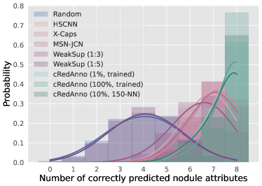
Figure 2: Probability of the number of correctly predicted nodule attributes. The probabilities of other methods are calculated using their reported prediction accuracy of individual nodule attributes, as in Tab. 1, where not-reported values are all assumed to be 100% accuracy. Observe that cRedAnno shows a significantly larger probability of simultaneously predicting all $8$ nodule attributes correctly.

The overall prediction performance is summarised in Tab. 1, comparing with the state-of-the-art. In summary, the results show that our proposed approach can reach simultaneously high accuracy in predicting malignancy and all nodule attributes. This increases the trustworthiness of the model significantly and has not been achieved by previous works. More specifically, when using only $1\%$ annotated samples, our approach achieves comparable or much higher accuracy compared with all previous works in predicting the nodule attributes. Meanwhile, the accuracy of predicting malignancy approaches X-Caps [15] and already exceeds HSCNN [22], which uses 3D volume data. Note that in this case we significantly outperform WeakSup(1:5) [13], which uses $100\%$ malignancy annotations and $16.7\%$ nodule attribute annotations. When using full annotation, our approach outperforms most of the other compared explainable methods in predicting malignancy and all nodule attributes, except “lobulation”, where ours is merely worse by absolute $0.6\%$ accuracy. It is worth mentioning that even in this case, we still use the fewest samples: only $518$ among the $730$ nodules are used for training. In addition, the consistent decent performance also indicates that our approach is reasonably robust w.r.t. to the value $k$ in k-NN classifiers.

To further validate the prediction performance of nodule attributes, for visual clarity, we select $3$ representative configurations of our proposed approach and compare them with others in Fig. 2. It can be clearly seen that using our approach, approximately $90\%$ nodules have at least $7$ attributes correctly predicted. In contrast, WeakSup(1:5) although reaches over $82.4\%$ accuracy in malignancy prediction, shows no significant difference compared to random guesses in predicting nodule attributes – this shows the opposite of trustworthiness.

3.2 Analysis of extracted features in learned space

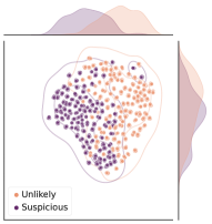
(a) Malignancy

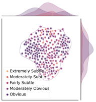
(b) Subtlety

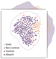
(c) Calcification

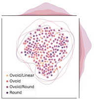
(d) Sphericity

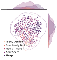
(e) Margin

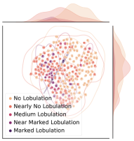
(f) Lobulation

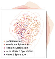
(g) Spiculation

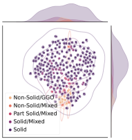
(h) Texture

Figure 3: t-SNE visualisation of features extracted from testing images. Data points are coloured using ground truth annotations. Malignancy shows highly separable in the learned space, and correlates with the clustering in each nodule attribute.

We hypothesise the superior performance of our proposed approach can attribute to the extracted features. So we use t-SNE [17] to further visualise the learned feature. Feature $f$ extracted from each testing image is mapped to a data point in 2D space. Fig. 3a to 3h correspond to these data points coloured by the ground truth annotations of malignancy to nodule attribute “texture”, respectively. Fig. 3a shows that the samples are reasonably linear-separable between the benign/malignant samples even in this dimensionality-reduced 2D space. This provides evidence of our good performance.

Furthermore, the correlation between the nodule attributes and malignancy can be found intuitively in Fig. 3. For example, the cluster in Fig. 3c indicates that solid calcification contributes negatively to malignancy. Similarly, the clusters in Fig. 3e and Fig. 3h indicate that poorly defined margin correlates with non-solid texture, and both of these contribute positively to malignancy. These findings are in accord with the diagnosis process of radiologists[28] and thus further support the trustworthiness of the proposed approach.

3.3 Ablation study

[] Arch #params Training strategy ImageNet pretrain Acc ResNet-50 23.5M end-to-end ✗ 86.74^$\ast$ two-stage ✗ 70.48 two-stage ✓ 70.48 ViT 21.7M end-to-end ✗ 64.24 two-stage ✗ 79.19 two-stage ✓ 88.30 $\ast$ This is a representative setting and performance of previous works using CNN architecture. []

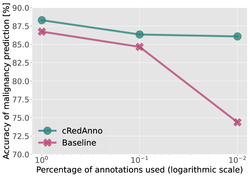
Figure 4: Accuracy of malignancy prediction ($\%$). All annotations are used during training. The highest accuracy is bolded. The result of our proposed setting is highlighted. Only cRedAnno and conventional end-to-end trained CNN achieve higher than $85\%$ accuracy.

Figure 5: Annotation reduction. Line colours correspond to settings in Tab. 5: “Baseline” uses ResNet-50 architecture and is trained end-to-end from random initialisation. cRedAnno shows strong robustness when annotation reduced.

3.3.1 Validation of components

We ablate our proposed approach by comparing with different architectures for encoders $E$, training strategies, and whether to use ImageNet-pretrained weights. The results in Tab. 5 show that ViT architecture benefits more from the self-supervised contrastive training compared to ResNet-50 as a CNN representative. This observation is in accord with the findings in [8, 6]. ViT’s lowest accuracy in end-to-end training reiterates its requirement for a large amount of training data [10]. Starting from the ImageNet-pretrained weights is also shown to be helpful for ViT but not ResNet-50, probably due to ViT’s lack of inductive bias needs far more than hundreds of training samples to compensate [10], especially for medical images. In summary, only the proposed approach and conventional end-to-end training of ResNet-50 achieve higher than $85\%$ accuracy of malignancy prediction.

3.3.2 Annotation reduction

We further plot the malignancy prediction accuracy of the aforementioned winners as the annotations are reduced on a logarithmic scale. As shown in Fig. 5, cRedAnno demonstrates strong robustness w.r.t. annotation reduction. The accuracy of the end-to-end trained ResNet-50 model decreases rapidly to $74.38\%$ when annotations reach only $1\%$. In contrast, the proposed approach still remains at $86.09\%$ accuracy, meanwhile high accuracy for predicting nodule attributes, as shown in Tab. 1.

4 Conclusion

In this study, we propose cRedAnno to considerably reduce the annotation need in predicting malignancy, meanwhile explaining nodule attributes for lung nodule diagnosis. Our experiments show that even with only $1\%$ annotation, cRedAnno can reach similar or better performance in predicting malignancy compared with state-of-the-art methods using full annotation, and significantly outperforms them in predicting nodule attributes. In addition, our proposed approach is the first to reach over $94\%$ accuracy in predicting all nodule attributes simultaneously. Visualisation of our extracted features provides novel evidence that in the learned space, the clustering of nodule attributes and malignancy is in accord with clinical knowledge of lung nodule diagnosis. Yet the limitations of this approach remain in its generalisability to be validated in other medical image analysis problems.

References

- [1] Al-Shabi, M., Lan, B.L., Chan, W.Y., Ng, K.H., Tan, M.: Lung nodule classification using deep Local–Global networks. International Journal of Computer Assisted Radiology and Surgery 14(10), 1815–1819 (Oct 2019). https://doi.org/10.1007/s11548-019-01981-7
- [2] Armato, S.G., McLennan, G., Bidaut, L., McNitt-Gray, M.F., et al.: The Lung Image Database Consortium (LIDC) and Image Database Resource Initiative (IDRI): A Completed Reference Database of Lung Nodules on CT Scans: The LIDC/IDRI thoracic CT database of lung nodules. Medical Physics 38(2), 915–931 (Jan 2011). https://doi.org/10.1118/1.3528204
- [3] Baltatzis, V., Bintsi, K.M., Folgoc, L.L., Martinez Manzanera, O.E., et al.: The Pitfalls of Sample Selection: A Case Study on Lung Nodule Classification. In: Predictive Intelligence in Medicine, vol. 12928, pp. 201–211. Springer International Publishing, Cham (2021). https://doi.org/10.1007/978-3-030-87602-919
- [4] Barredo Arrieta, A., Díaz-Rodríguez, N., Del Ser, J., Bennetot, A., et al.: Explainable Artificial Intelligence (XAI): Concepts, taxonomies, opportunities and challenges toward responsible AI. Information Fusion 58, 82–115 (Jun 2020). https://doi.org/10.1016/j.inffus.2019.12.012
- [5] Caron, M., Misra, I., Mairal, J., Goyal, P., et al.: Unsupervised learning of visual features by contrasting cluster assignments. In: Advances in Neural Information Processing Systems. vol. 33, pp. 9912–9924. Curran Associates, Inc. (2020)
- [6] Caron, M., Touvron, H., Misra, I., Jégou, H., et al.: Emerging Properties in Self-Supervised Vision Transformers. In: Proceedings of the IEEE/CVF International Conference on Computer Vision. pp. 9650–9660 (2021)
- [7] Chen, W., Wang, Q., Yang, D., Zhang, X., et al.: End-to-End Multi-Task Learning for Lung Nodule Segmentation and Diagnosis. In: 2020 25th International Conference on Pattern Recognition (ICPR). pp. 6710–6717. IEEE, Milan, Italy (Jan 2021). https://doi.org/10.1109/ICPR48806.2021.9412218
- [8] Chen, X., Xie, S., He, K.: An Empirical Study of Training Self-Supervised Vision Transformers. In: 2021 IEEE/CVF International Conference on Computer Vision (ICCV). pp. 9620–9629. IEEE, Montreal, QC, Canada (Oct 2021). https://doi.org/10.1109/ICCV48922.2021.00950
- [9] del Ciello, A., Franchi, P., Contegiacomo, A., Cicchetti, G., et al.: Missed lung cancer: When, where, and why? Diagnostic and Interventional Radiology 23(2), 118–126 (Mar 2017). https://doi.org/10.5152/dir.2016.16187
- [10] Dosovitskiy, A., Beyer, L., Kolesnikov, A., Weissenborn, D., et al.: An Image is Worth 16x16 Words: Transformers for Image Recognition at Scale. In: International Conference on Learning Representations (Sep 2020)
- [11] Grill, J.B., Strub, F., Altché, F., Tallec, C., et al.: Bootstrap Your Own Latent - A New Approach to Self-Supervised Learning. In: Advances in Neural Information Processing Systems. vol. 33, pp. 21271–21284. Curran Associates, Inc. (2020)
- [12] He, K., Fan, H., Wu, Y., Xie, S., Girshick, R.: Momentum Contrast for Unsupervised Visual Representation Learning. In: 2020 IEEE/CVF Conference on Computer Vision and Pattern Recognition (CVPR). pp. 9726–9735. IEEE, Seattle, WA, USA (Jun 2020). https://doi.org/10.1109/CVPR42600.2020.00975
- [13] Joshi, A., Sivaswamy, J., Joshi, G.D.: Lung nodule malignancy classification with weakly supervised explanation generation. Journal of Medical Imaging 8(04) (Aug 2021). https://doi.org/10.1117/1.JMI.8.4.044502
- [14] Kazerooni, E.A., Austin, J.H., Black, W.C., Dyer, D.S., et al.: ACR–STR Practice Parameter for the Performance and Reporting of Lung Cancer Screening Thoracic Computed Tomography (CT): 2014 (Resolution 4)*. Journal of Thoracic Imaging 29(5), 310–316 (Sep 2014). https://doi.org/10.1097/RTI.0000000000000097
- [15] LaLonde, R., Torigian, D., Bagci, U.: Encoding Visual Attributes in Capsules for Explainable Medical Diagnoses. In: Medical Image Computing and Computer Assisted Intervention – MICCAI 2020. pp. 294–304. Lecture Notes in Computer Science, Springer International Publishing, Cham (2020). https://doi.org/10.1007/978-3-030-59710-829
- [16] Liu, L., Dou, Q., Chen, H., Qin, J., Heng, P.A.: Multi-Task Deep Model With Margin Ranking Loss for Lung Nodule Analysis. IEEE Transactions on Medical Imaging 39(3), 718–728 (Mar 2020). https://doi.org/10.1109/TMI.2019.2934577
- [17] van der Maaten, L., Hinton, G.: Visualizing Data using t-SNE. Journal of Machine Learning Research 9(86), 2579–2605 (2008)
- [18] Rudin, C.: Stop explaining black box machine learning models for high stakes decisions and use interpretable models instead. Nature Machine Intelligence 1(5), 206–215 (May 2019). https://doi.org/10.1038/s42256-019-0048-x
- [19] Russakovsky, O., Deng, J., Su, H., Krause, J., et al.: ImageNet Large Scale Visual Recognition Challenge. International Journal of Computer Vision 115(3), 211–252 (Dec 2015). https://doi.org/10.1007/s11263-015-0816-y
- [20] Salahuddin, Z., Woodruff, H.C., Chatterjee, A., Lambin, P.: Transparency of deep neural networks for medical image analysis: A review of interpretability methods. Computers in Biology and Medicine 140, 105111 (Jan 2022). https://doi.org/10.1016/j.compbiomed.2021.105111
- [21] Salimans, T., Kingma, D.P.: Weight Normalization: A Simple Reparameterization to Accelerate Training of Deep Neural Networks. In: Advances in Neural Information Processing Systems. vol. 29. Curran Associates, Inc. (2016)
- [22] Shen, S., Han, S.X., Aberle, D.R., Bui, A.A., Hsu, W.: An interpretable deep hierarchical semantic convolutional neural network for lung nodule malignancy classification. Expert Systems with Applications 128, 84–95 (Aug 2019). https://doi.org/10.1016/j.eswa.2019.01.048
- [23] Stammer, W., Schramowski, P., Kersting, K.: Right for the Right Concept: Revising Neuro-Symbolic Concepts by Interacting with their Explanations. In: 2021 IEEE/CVF Conference on Computer Vision and Pattern Recognition (CVPR). pp. 3618–3628. IEEE, Nashville, TN, USA (Jun 2021). https://doi.org/10.1109/CVPR46437.2021.00362
- [24] Tjoa, E., Guan, C.: A Survey on Explainable Artificial Intelligence (XAI): Toward Medical XAI. IEEE Transactions on Neural Networks and Learning Systems 32(11), 4793–4813 (Nov 2021). https://doi.org/10.1109/TNNLS.2020.3027314
- [25] Touvron, H., Cord, M., Douze, M., Massa, F., et al.: Training data-efficient image transformers & distillation through attention. In: Proceedings of the 38th International Conference on Machine Learning. pp. 10347–10357. PMLR (Jul 2021)
- [26] van der Velden, B.H., Kuijf, H.J., Gilhuijs, K.G., Viergever, M.A.: Explainable artificial intelligence (XAI) in deep learning-based medical image analysis. Medical Image Analysis 79, 102470 (Jul 2022). https://doi.org/10.1016/j.media.2022.102470
- [27] Vaswani, A., Shazeer, N., Parmar, N., Uszkoreit, J., et al.: Attention is All you Need. In: Advances in Neural Information Processing Systems. vol. 30. Curran Associates, Inc. (2017)
- [28] Vlahos, I., Stefanidis, K., Sheard, S., Nair, A., et al.: Lung cancer screening: Nodule identification and characterization. Translational Lung Cancer Research 7(3), 288–303 (Jun 2018). https://doi.org/10.21037/tlcr.2018.05.02