Data-driven Thiele equation approach for solving the full nonlinear spin-torque vortex oscillator dynamics

Abstract

The dynamics of vortex based spin-torque nano-oscillators is investigated theoretically. Starting from a fully analytical model based on the Thiele equation approach, fine-tuned data-driven corrections are carried out to the gyrotropic and damping terms. These adjustments, based on micromagnetic simulation results, allow to quantitatively model the response of such oscillators to any dc current within the range of the vortex stability. Both, the transient and the steady-state regimes are accurately predicted under the proposed data-driven Thiele equation approach. Furthermore, the computation time required to solve the dynamics of such system is reduced by about six orders of magnitude compared to the most powerful micromagnetic simulations. This major breakthrough opens the path for unprecedented high-throughput simulations of spin-torque vortex oscillators submitted to long-duration input signals, for example in neuromorphic computing applications.

I Introduction

Artificial neural network (ANN) algorithms have emerged as one of the most successful machine learning paradigms in recent years Hopfield (1988); Thrun (1994); Jain et al. (1996); Silver et al. (2017); Jumper et al. (2021). However typical software implementation of ANNs are generally energy-consuming, driving the seek for low-power solutions. In this framework, neuromorphic computing aims to draw inspiration from the human brain architecture to propose energy efficient hardware implementations of ANNs capable of solving complex cognitive tasks. Different physical devices mimicking neuronal properties have been considered up to now, such as memristors Milano et al. (2021) or transistors Roy et al. (2019). All are characterized by a nonlinear response to a given stimulus, analogously to their biological equivalent. Among other implementations explored, spin-torque vortex oscillators (STVOs) present many advantages, such as nanoscale, low-noise and great tunability Pribiag et al. (2007). These devices, based on magnetic tunnel junctions (MTJs) in which the free ferromagnetic layer hosts a non-uniform magnetic vortex state, have already shown convincing results in various speech recognition applications Torrejon et al. (2017); Romera et al. (2018).
Different approaches exist for modeling the dynamics of magnetic vortices. Among these, the micromagnetics formalism is well-recognized to give quantitative results comparable to experimental measurements Leliaert and Mulkers (2019). Based on a continuum approximation, it consists in solving time-dependent equations of magnetization dynamics. Despite the accuracy of their results, micromagnetic simulations (MMS) present the main disadvantage of requiring important computational power as well as being time-consuming. This makes them ineffective for handling any signal encountered in practical applications. An alternative is to use analytical equations, much faster to solve, describing the vortex motion. For example, very simple models (i.e., exponential decay) have already been used to approximate the vortex core displacement in transient regime of oscillation Abreu Araujo et al. (2020). More commonly, the Thiele equation approach Thiele (1973) (TEA) is examined. Albeit based on physical considerations, it has though given poor results compared to simulations up until now because of cumbersome mathematical derivations involved for a vortex topology.

In this work, we propose a new hybrid method (i.e., semi-analytical) which is both fast and accurate to describe the vortex core precessions. Based on a small set of simulations which have reached steady-state oscillating regime, we can adapt the gyrotropic and damping terms appearing in the Thiele equation. This allows to capture the STVO response to any current of arbitrary form in transient and steady-state oscillating regime. We show that this technique can accelerate the computation time by several orders of magnitude compared to micromagnetism, while remaining as precise.

II Methods

The dynamics of vortices confined inside ferromagnetic nanopillars can be described using the Thiele equation approach Thiele (1973). The case of a free layer of radius $R$ and thickness $h$ will be considered hereafter. Within this framework, the vortex core is seen as a quasi-particle and identified by its in-plane position $\mathbf{X}=(X,Y)$ inside the cylindrical dot. Following the TEA, the evolution of the vortex core position is given as

$$G(\mathbf{e}_{z}\times\dot{\mathbf{X}})+D\dot{\mathbf{X}}=\frac{\partial W}{\partial\mathbf{X}}+\mathbf{F}^{\text{ST}},$$ (1)

where $G$ and $D$ are the gyrotropic and damping constants, respectively, $W$ is the potential magnetic energy associated to a displacement of the vortex core and $\mathbf{F}^{\text{ST}}$ are the forces related to the spin-transfer torque. In a previous work Abreu Araujo et al. (2022) we showed that, considering a perpendicular polarizer, Eq. (1) could be reduced to the following system of linear first-order differential equations

$$\left[{\begin{array}[]{c}\dot{X}\\ \dot{Y}\\ \end{array}}\right]=\underbrace{\left[{\begin{array}[]{cc}\Gamma&-\omega\\ \omega&\Gamma\\ \end{array}}\right]}_{\bar{\bar{\Omega}}}\left[{\begin{array}[]{c}X\\ Y\\ \end{array}}\right],$$ (2)

where the parameters $\Gamma$ and $\omega$ are given as

$$\Gamma =\frac{D(k^{\text{ex}}+k^{\text{ms}}+CJ_{\text{dc}}\kappa^{\text{Oe}})+GJ_{\text{dc}}\kappa^{\text{ST}}_{\perp}}{D^{2}+G^{2}},$$ (3)

$$\omega =\frac{DJ_{\text{dc}}\kappa^{\text{ST}}_{\perp}-G(k^{\text{ex}}+k^{\text{ms}}+CJ_{\text{dc}}\kappa^{\text{Oe}})}{D^{2}+G^{2}},$$ (4)

where $C=\pm 1$ is the vortex chirality and $J_{\text{dc}}$ the direct current density. The other terms are explicited hereafter.

In this simple harmonic oscillator model, we considered three contributions to $W$, namely the exchange, magneto-static and Ampère-Oersted field energies. Those are expressed using their spring-like restoring force constants $k$ as

$$\frac{\partial W}{\partial\mathbf{X}}=(k^{\text{ex}}+k^{\text{ms}}+\underbrace{CJ_{\text{dc}}\kappa^{\text{Oe}}}_{k^{\text{Oe}}})\mathbf{X}.$$ (5)

Here and below, the notation $s=\sqrt{X^{2}+Y^{2}}/R$ will be used to refer to the vortex core reduced position. The exchange energy contribution writes as Guslienko et al. (2001); Gaididei et al. (2010)

$$k^{\text{ex}}=(2\pi)^{2}hM_{\text{s}}^{2}(l_{\text{ex}}/R)^{2}/(1-s^{2}),$$ (6)

where $M_{\text{s}}$ is the saturation magnetization and $l_{\text{ex}}=\sqrt{A/(2\pi M_{\text{s}}^{2})}$ is the exchange length of the material, with $A$ the exchange stiffness coefficient. The magneto-static component is given as Gaididei et al. (2010); Abreu Araujo et al. (2022)

$$k^{\text{ms}}_{\xi}=\frac{8M_{\text{s}}^{2}h^{2}}{R}\textstyle\Lambda_{0,\xi}\left(1+a_{\xi}s^{2}+b_{\xi}s^{4}+c_{\xi}s^{6}\right),$$ (7)

where $\xi=h/(2R)$ corresponds to the aspect ratio of the nanodot. The parameters $\Lambda_{0,\xi}$, $a_{\xi}$, $b_{\xi}$ and $c_{\xi}$ can be calculated thanks to numerical methods we described in Abreu Araujo et al. (2022). Finally, the contribution related to the Ampère-Oersted field has been derived as follows Abreu Araujo et al. (2022)

$$\kappa^{\text{Oe}}=\frac{8\pi^{2}}{75}M_{\text{s}}Rh\left(1-\frac{4}{7}s^{2}-\frac{1}{7}s^{4}-\frac{16}{231}s^{6}-\frac{125}{3003}s^{8}\right).$$ (8)

In the absence of any external magnetic field, the latter accounts for the entire Zeeman energy.

As stated previously, we fixed the polarization direction to be out-of-plane. This means that only the perpendicular component of the Slonczewski spin-torque Slonczewski (1996) contributes to the STVO dynamics. We have thus $\mathbf{F}^{\text{ST}}=\kappa^{\text{ST}}_{\perp}J_{\text{dc}}(\mathbf{e}_{z}\times\mathbf{X})$ with Khvalkovskiy et al. (2009); Dussaux et al. (2012)

$$\kappa^{\text{ST}}_{\perp}=\pi a_{J}M_{\text{s}}hp_{z},$$ (9)

where $\mathbf{p}=p_{z}\mathbf{e}_{z}=(0,0,1)$ is the unit vector giving the polarization direction of the fixed layer, $a_{J}=p_{J}\hbar/(2|e|M_{\text{s}}^{\text{ref}}h)$ is the spin-transfer efficiency with $p_{J}$ the spin-current polarization, $e$ is the electron charge and $M_{\text{s}}^{\text{ref}}$ the polarizer saturation magnetization.

In our previous model, we supposed that the gyro- and damping constants were independent of the vortex core position. We had thus $G=G_{0}=-2\pi PM_{\text{s}}h/\gamma_{\text{G}}$ Guslienko et al. (2002); Guslienko (2006), where $P$ is the vortex polarity and $\gamma_{\text{G}}=g|e|/(2m_{e})$ is the gyromagnetic ratio with $g$ the electron spin $g$-factor and $m_{e}$ the electron mass, and $D=D_{0}=-\alpha_{\text{G}}\eta|G|$ with $\alpha_{\text{G}}$ the Gilbert damping constant and $\eta=\ln(R/(2l_{\text{ex}}))/2+3/8$ Khvalkovskiy et al. (2009). This assumption led to quantitative predictions in the resonant regime (i.e., $s=0$) but lack of precision for nonlinear auto-oscillations. In the present paper we propose to take the $s$-dependence of $G(s)$ and $D(s)$ into account.

As the calculation of the latter is a very difficult task, no convincing expression exists in the literature, to the best of our knowledge, to describe their evolution with respect to the core position. Thence, we chose a more convenient approach. The gyro- and damping terms are modeled as $G(s)=G_{0}f_{G}(s)$ and $D(s)=D_{0}f_{D}(s)$, respectively. The functions $f_{G}(s)$ and $f_{D}(s)$ are supposed to be even power expansions of $s$, so that

$$f_{G}(s) =1+a_{G}s^{2}+b_{G}s^{4}+c_{G}s^{6}+d_{G}s^{8},$$ (10)

$$f_{D}(s) =1+a_{D}s^{2}+b_{D}s^{4}+c_{D}s^{6}+d_{D}s^{8}.$$ (11)

This definition allows to retrieve $G(0)=G_{0}$ and $D(0)=D_{0}$, as $f_{G}(0)=1$ and $f_{D}(0)=1$. In addition, the coefficients appearing in Eqs (10) & (11) can be deduced from a limited set of simulations. By fitting micromagnetic results to our analytical model, it is thus possible to considerably enhance its predictions for $s\neq 0$. This step is performed by following the procedure described hereafter.

Using the matrix $\bar{\bar{\Omega}}$ from Eq. (2), the following system is derived

$$\begin{cases}D(s)\Gamma-G(s)\omega=k^{\text{ex}}(s)+k^{\text{ms}}(s)+CJ_{\text{dc}}\kappa^{\text{Oe}}(s)\\ D(s)\omega+G(s)\Gamma=J_{\text{dc}}\kappa^{\text{ST}}_{\perp}\end{cases}$$ (12)

As $\Gamma=0$ in steady-state oscillating regime Abreu Araujo et al. (2022) and using the expressions of $G(s)$ and $D(s)$, one finds

$$\delta_{G}f_{G}(s) =-\frac{k^{\text{ex}}(s)+k^{\text{ms}}(s)+CJ_{\text{dc}}\kappa^{\text{Oe}}(s)}{G_{0}\omega(s)},$$ (13)

$$\delta_{D}f_{D}(s) =\frac{J_{\text{dc}}\kappa^{\text{ST}}_{\perp}}{D_{0}\omega(s)},$$ (14)

where we introduced two global correction factors $\delta_{G}$ and $\delta_{D}$. Those aim to absorb any imprecision of the model resulting from the multiple assumptions made, even at $s=0$. Those discrepancies could originate from the analytical expression of $G_{0}$ and $D_{0}$ as well as from the other terms at $s=0$, i.e., $k^{\text{ex}}_{0}$, $k^{\text{ms}}_{0}$ $\kappa^{\text{Oe}}_{0}$ or $\kappa^{\text{ST}}_{\perp}$.

The only remaining unknown parameter in Eqs. (13) & (14) is the angular frequency $\omega(s)$. Fortunately it can simply be extracted from micromagnetic simulations having reached steady-state regime, as $\omega(s)=2\pi f(s)$. Thus, one can easily model $G(s)$ and $D(s)$ by performing a fit on several simulation results. Let us precise that generally, the input variable of micromagnetic solvers is the injected current. We then obtain $\omega(J_{\text{dc}})$ as well as $s(J_{\text{dc}})$, involving a supplementary substitution.

Micromagnetic simulations are performed using mumax³, a GPU-based program Vansteenkiste et al. (2014), following the same protocol as for our previous study Abreu Araujo et al. (2022). A free layer made of permalloy, with a radius $R$ of 100 nm and a thickness $h$ of 10 nm is considered. The used material parameters are presented in Table 1. The magnetic dot is discretized into $2.5\times 2.5$ nm² cells and two layers with a thickness of 5 nm each. Current densities ranging from 0 to 10 MA/cm² are injected into the junction, in the positive $z$-direction. The vortex polarity $P$ is thus fixed at -1, to respect the condition for stable auto-oscillations, i.e., $J_{\text{dc}}Pp_{z}<0$.

Table 1: Material parameters of the magnetic tunnel junctions considered in the micromagnetic simulations and the analytical model.

Parameter	Symbol	Value	Units
Saturation magnetization	$M_{\text{s}}=M_{\text{s}}^{\text{ref}}$	800	emu/cm3
Exchange stiffness coefficient	$A$	1.07$\cdot 10^{-6}$	erg/cm
Gilbert damping constant	$\alpha_{\text{G}}$	0.01	-
Spin-current polarization	$p_{J}$	0.2	-

Suitable physical simulation time is chosen to reach steady-state regime for each current. The reduced orbit radius $s$ is internally computed by mumax³, while the frequency is retrieved thanks to our SNIFA technique Abreu Araujo (2021). Magneto-crystalline anisotropy and the effect of temperature are neglected in this study. Three chiral configurations are examined, depicting the impact of the Ampère-Oersted field (AOF) $\mathbf{H}_{\text{Oe}}$ on the STVO dynamics: one without taking $\mathbf{H}_{\text{Oe}}$ into account, one with the planar vortex magnetization parallel to $\mathbf{H}_{\text{Oe}}$ ($C=+1$) and one anti-parallel to $\mathbf{H}_{\text{Oe}}$ ($C=-1$). Those will be labelled as noOe, $C^{+}$ and $C^{-}$, respectively.

III Results & Discussion

The intrinsic property of our STVO, namely its gyrotropic frequency $f(s)=\omega(s)/(2\pi)$ with respect to the reduced orbit radius $s$, is presented on Fig. 1. Those micromagnetic simulation data correspond only to the steady-state oscillating regime, i.e., $s\in]0,0.8]$. To increase the number of data points available for the fit, we performed a cubic interpolation on simulation results. Obviously, different sets of fitting coefficients (see Eqs. (10) & (11)) are derived for each chiral configuration. Also, the fitting bounds are chosen such as to stay in the nonlinear steady-state oscillating regime. The frequency retrieved from mumax³ was originally expressed as $\omega(J_{\text{dc}})$. However, as we also obtained the evolution of $s(J_{\text{dc}})$ with respect to the current density Abreu Araujo et al. (2022), we can easily express Eqs. (13) & (14) as either being $s$ or $J_{\text{dc}}$ dependent. Data points starting from 5.8, 6.2, 6.5 MA/cm² and ending at 8.4, 9, 9.8 MA/cm² were examined for $C^{-}$, noOF and $C^{+}$, respectively. Those current densities range thus between the first and second corresponding critical currents $J_{\text{c1}}$ and $J_{\text{c2}}$ Abreu Araujo et al. (2022).

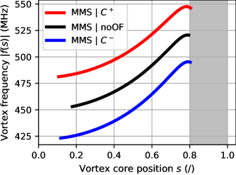
Figure 1: Absolute vortex gyrotropic frequency $|f(s)|$ as a function of the reduced vortex core position $s$, obtained from micromagnetic simulations (MMS). The colours black, red and blue correspond to simulations without AOF (noOF), with AOF and $C=+1$ ($C^{+}$) and with AOF and $C=-1$ ($C^{-}$), respectively. Only data in the steady-state oscillating regime are shown here, i.e., $s\in]0,0.8]$. Cubic interpolations of the data points are depicted here with the respective color lines. The grey area represents the limit of vortex stability.

Since the evolution of the angular frequency $\omega(s)$ is known thanks to the simulations, the right hand side of Eq. (13) can be determined for any value of $s$. A nonlinear least squares method is then used to fit the polynomial function proposed in Eq. (10). The obtained coefficients are reported in Table 2. As stated previously a global correction factor $\delta_{G}$ is also introduced to take into account any discrepancies between the fully analytical TEA model and the MMS results, even in the resonant regime (i.e., $s=0$). One can observe that $\delta_{G}>1$ for the three configurations which could either indicate an underestimation of the gyroconstant $G_{0}$ or an overestimation of the stiffness parameters term $k^{\text{ex}}+k^{\text{ms}}+CJ_{\text{dc}}\kappa^{\text{Oe}}$.

Table 2: Coefficients of the polynomial function given in Eq. (10), for each chiral configuration. Those were calculated from Eq. (13) by a least squares nonlinear fit, after a cubic interpolation on the micromagnetic simulation data as presented on Fig. 1. The maximum relative error between fit and simulation is also indicated.

	$\delta_{G}$	$a_{G}$	$b_{G}$	$c_{G}$	$d_{G}$	max($|$err$|$) [%]
$C^{+}$	1.0904	-0.0347	0.5118	-1.5998	1.8183	0.328
noOF	1.0977	-0.0504	0.5799	-1.7092	1.8900	0.241
$C^{-}$	1.1054	-0.0417	0.5835	-1.8082	2.0513	0.355

The evolution of the $\delta_{G}f_{G}(s)$ function with respect to the input dc current density $J_{\text{dc}}$ is depicted on Fig. 2. Continuously increasing nonlinear curves are obtained. The compensation of the exchange component could especially become dominant for high currents, as it diverges for value of $s\rightarrow 1$ (see Eq. (6)). A strong splitting between the three configurations is noticed. This observation, which will be the subject of a future communication, could indicate that the chirality has an influence on the potential magnetic energy terms. As demonstrated in previous works Khvalkovskiy et al. (2009); Abreu Araujo et al. (2022); Abreu Araujo and Grollier (2016); Choi et al. (2009), the Zeeman term sign is directly impacted by the direction of the Ampère-Oersted field. However such splitting effect is not straightforward concerning the exchange and magneto-static terms.

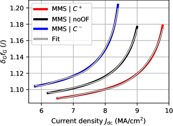
Figure 2: Value of $\delta_{G}f_{G}(s)$ as a function of the input dc current density $J_{\text{dc}}$ for each chiral configuration $C^{+}$, noOF and $C^{-}$, identified in red, black and blue colors, respectively. The results calculated from Eq. (13) (colored lines) were obtained after a cubic interpolation performed on the micromagnetic simulation (MMS) data presented on Fig. (1). The corresponding polynomial fits (see Eq. (10)) are represented with white lines.

An identical protocol is used to extract the $s$-dependence of the damping term. Knowing $\omega(s)$, the right hand side of Eq. (14) can be calculated. Once fitted to the polynomial function given in Eq. (11), the coefficients reported in Table 3 are obtained. As for the gyrotropic term, one can observe that the global correction factor $\delta_{D}>1$, reporting either a too important $J_{\text{dc}}\kappa^{\text{ST}}_{\perp}$ value or an underestimated damping constant $D_{0}$ when the vortex core is at the center of the dot.

Table 3: Coefficients of the polynomial function given in Eq. (11), for each chiral configuration. Those were calculated from Eq. (14) by a least squares nonlinear fit, after a cubic interpolation on the micromagnetic simulation data as presented on Fig. 1. The maximum relative error between fit and simulation is also indicated.

	$\delta_{D}$	$a_{D}$	$b_{D}$	$c_{D}$	$d_{D}$	max($|$err$|$) [%]
$C^{+}$	1.0267	0.3499	0.1220	0.1790	0.0494	0.058
noOF	1.0345	0.3017	0.1112	0.1301	0.0513	0.026
$C^{-}$	1.0423	0.2629	0.0793	0.1412	0.0168	0.030

The value of $\delta_{D}f_{D}(s)$ as a function of $J_{\text{dc}}$ is given on Fig. 3. A much more linear evolution is reported, compared to $\delta_{G}f_{G}(s)$ (see Fig. 2). Again, a clear splitting between the three configurations is noticed. As it was the case for $\delta_{G}f_{G}(s)$, the respective distances between the $C^{+}$ and $C^{-}$ cases and the noOF curve is different which confirm the strong nonlinear behavior of the STVO dynamics.

As data-driven corrections have been made to the TEA model (i.e., $G(s)$ and $D(s)$), we can now use it to predict the dynamics of our STVO with new input dc current density values by simply solving the system given in Eq. (2). This novel hybrid method, which is semi-analytical, will be referred to as the data-driven Thiele equation approach (DD-TEA). A comparison between mumax³ simulations and our DD-TEA model for the reduced vortex core position $s(t)$ and instantaneous frequency $f(t)$ with respect to time is given on Fig. 4. The input currents were chosen to be between the two critical currents $J_{\text{c1}}$ and $J_{\text{c2}}$. The steady-state core position values are completely overlapped for both methods, even for $J_{\text{dc}}=9$ MA/cm² which leads to $s\approx 0.8$, i.e., the limit of the model validity (but also the limit corresponding to the vortex polarity switch). Regarding the frequency, all curves start at $f\approx-449$ MHz. This frequency correspond to a vortex core position of $s=0.01$, the starting point of the simulations. As this orbit is close to $s=0$, the frequency is almost equal to $\omega_{0}/(2\pi)$ Abreu Araujo et al. (2022). With time increasing, the frequency evolves to the steady-state value corresponding to the current imposed. Various works Gaididei et al. (2010); Dussaux et al. (2012); Choi et al. (2009) propose TEA-based predictions of the steady-state orbit of oscillation and/or the frequency but rarely with such quantitative agreement, due to the lack of consideration of high-order terms. As far as the transient regime is concerned, only Guslienko et al. proposed a satisfactory analytical equation Guslienko et al. (2014), to the best of our knowledge. In the present work, perfect correspondence is obtained. Relaxation time are consistent with simulations. This is not straightforward as only steady-state results were used to calibrate the model. Nothing but negligible shift between both methods is remarked in the transition for the lowest current curves.

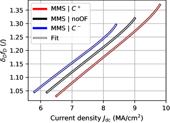
Figure 3: Value of $\delta_{D}f_{D}(s)$ as a function of the input dc current density $J_{\text{dc}}$ for each chiral configuration $C^{+}$, noOF and $C^{-}$, identified in red, black and blue colors, respectively. The results calculated from Eq. (14) (colored lines) were obtained after a cubic interpolation performed on the micromagnetic simulation (MMS) data presented on Fig. (1). The corresponding polynomial fits (see Eq. (11)) are represented with white lines.

Numerically solving the STVO dynamics using mumax³ for 2000 ns, as presented in Fig. 4, takes no less than three hours with the most powerful hardware to date (NVIDIA Tesla A100 GPU). Using now our DD-TEA model this calculation time is reduced to about 13 ms, an acceleration of more than 700k times. This number overcomes largely the already great 200 factor recently brought up by Chen et al. Chen et al. (2022) for solving similar problems using artificial intelligence techniques. This remarkable speed-up can be explained by a dramatic reduction of the number of equations to be solved when using the DD-TEA instead of micromagnetic simulations. In mumax³, the Landau-Lifshitz-Gilbert-Slonczewski Landau and Lifshitz (1992); Gilbert (2004); Slonczewski (1996) equation is calculated in each cell of the magnetic structure, for each time step in the three spatial directions. For the specific dimensions used in this study, it corresponds to numerically solve 30144 equations between each timestep. Regarding the DD-TEA, only two equations are required, one for each in-plane coordinate of the vortex core, as the latter is seen as a quasi-particle. Furthermore, we believe that the speed-up factor obtained in this work would be further increased if our DD-TEA homemade code, for now running on a single CPU core, could be optimized to run on highly parallel GPU hardware. In addition, for larger radius dots even better numbers are expected as the number of cells scales up proportionally to $R^{2}$, for the same unit cell dimensions. Preliminary tests performed on a nanodot presenting a radius $R$ of 500 nm and a thickness $h$ of 9 nm (with same planar unit cell dimensions than for the present study) have given a speed-up factor of more than 2M times.

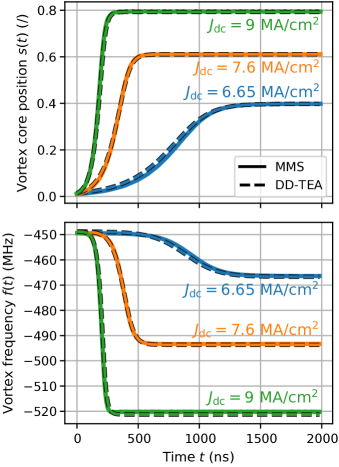
Figure 4: Transient regime calculations using micromagnetic simulations (MMS - continuous lines) and data-driven Thiele equation approach (DD-TEA - dashed lines) for (top) the reduced vortex core position $s(t)$ and (bottom) the vortex oscillation frequency $f(t)$. The input dc current densities $J_{\text{dc}}$ applied are 6.65, 7.6 and 9 MA/cm² in blue, orange and green, respectively. The Ampère-Oersted field was not taken into account. All simulations were started at $s=0.01$.

IV Conclusion

The dynamics of spin-torque vortex oscillators under out-of-plane input dc currents has been investigated. Starting from a fully analytical Thiele equation approach model developed previously Abreu Araujo et al. (2022), data-driven corrections were brought to the gyrotropic and damping terms. These adjustments were obtained by fitting the model predictions to micromagnetic results performed using mumax³. This hybrid method was then used to compute the STVO dynamics for new input current values and compared to micromagnetic predictions. An unprecedented agreement between both methods has been shown in the steady-state as well as in the transient regime. In addition to its accuracy, the DD-TEA model is faster than mumax³ by a factor of about 1 million although the micromagnetic simulations were performed using the most powerful hardware available to date (NVIDIA Tesla A100 GPGPUs). Up to now, simulating STVO response for long-duration input signals was impractical as no method existed for performing both fast and precise simulations. The results presented in this paper fulfill both requirements and open the way for pioneering functionalization of such oscillators, namely in the framework of neuromorphic computing applications.

V Acknowledgements

Computational resources have been provided by the Consortium des Équipements de Calcul Intensif (CÉCI), funded by the Fonds de la Recherche Scientifique de Belgique (F.R.S.-FNRS) under Grant No. 2.5020.11 and by the Walloon Region. F.A.A. is a Research Associate of the F.R.S.-FNRS. S.d.W. aknowledges the Walloon Region and UCLouvain for FSR financial support.

VI Author contributions statement

The study was designed by F.A.A. who created the analytical model. F.A.A. designed the micromagnetic simulations performed by S.d.W. and C.C.. S.d.W. wrote the core of the manuscript and all the co-authors (F.A.A., S.d.W. and C.C.) contributed to the text as well as to the analysis of the results.

VII Data Availability

The datasets generated during and/or analyzed during the current study are available from the corresponding author on reasonable request.

VIII Additional information

The authors declare no competing interests.

References

- Hopfield (1988) J. J. Hopfield, IEEE Circuits and Devices Magazine 4, 3 (1988).
- Thrun (1994) S. Thrun, Advances in neural information processing systems 7 (1994).
- Jain et al. (1996) A. K. Jain, J. Mao, and K. M. Mohiuddin, Computer 29, 31 (1996).
- Silver et al. (2017) D. Silver, J. Schrittwieser, K. Simonyan, I. Antonoglou, A. Huang, A. Guez, T. Hubert, L. Baker, M. Lai, A. Bolton, et al., nature 550, 354 (2017).
- Jumper et al. (2021) J. Jumper, R. Evans, A. Pritzel, T. Green, M. Figurnov, O. Ronneberger, K. Tunyasuvunakool, R. Bates, A. Žídek, A. Potapenko, et al., Nature 596, 583 (2021).
- Milano et al. (2021) G. Milano, G. Pedretti, K. Montano, S. Ricci, S. Hashemkhani, L. Boarino, D. Ielmini, and C. Ricciardi, Nature Materials , 1 (2021).
- Roy et al. (2019) K. Roy, A. Jaiswal, and P. Panda, Nature 575, 607 (2019).
- Pribiag et al. (2007) V. Pribiag, I. Krivorotov, G. Fuchs, P. Braganca, O. Ozatay, J. Sankey, D. Ralph, and R. Buhrman, Nature physics 3, 498 (2007).
- Torrejon et al. (2017) J. Torrejon, M. Riou, F. Abreu Araujo, S. Tsunegi, G. Khalsa, D. Querlioz, P. Bortolotti, V. Cros, K. Yakushiji, A. Fukushima, et al., Nature 547, 428 (2017).
- Romera et al. (2018) M. Romera, P. Talatchian, S. Tsunegi, F. Abreu Araujo, V. Cros, P. Bortolotti, J. Trastoy, K. Yakushiji, A. Fukushima, H. Kubota, et al., Nature 563, 230 (2018).
- Leliaert and Mulkers (2019) J. Leliaert and J. Mulkers, Journal of Applied Physics 125, 180901 (2019).
- Abreu Araujo et al. (2020) F. Abreu Araujo, M. Riou, J. Torrejon, S. Tsunegi, D. Querlioz, K. Yakushiji, A. Fukushima, H. Kubota, S. Yuasa, M. D. Stiles, et al., Scientific reports 10, 1 (2020).
- Thiele (1973) A. Thiele, Physical Review Letters 30, 230 (1973).
- Abreu Araujo et al. (2022) F. Abreu Araujo, C. Chopin, and S. de Wergifosse, Scientific Reports 12, 10605 (2022).
- Guslienko et al. (2001) K. Y. Guslienko, V. Novosad, Y. Otani, H. Shima, and K. Fukamichi, Applied Physics Letters 78, 3848 (2001).
- Gaididei et al. (2010) Y. Gaididei, V. P. Kravchuk, and D. D. Sheka, International Journal of Quantum Chemistry 110, 83 (2010).
- Slonczewski (1996) J. C. Slonczewski, Journal of Magnetism and Magnetic Materials 159, L1 (1996).
- Khvalkovskiy et al. (2009) A. Khvalkovskiy, J. Grollier, A. Dussaux, K. A. Zvezdin, and V. Cros, Physical Review B 80, 140401 (2009).
- Dussaux et al. (2012) A. Dussaux, A. Khvalkovskiy, P. Bortolotti, J. Grollier, V. Cros, and A. Fert, Physical Review B 86, 014402 (2012).
- Guslienko et al. (2002) K. Y. Guslienko, B. Ivanov, V. Novosad, Y. Otani, H. Shima, and K. Fukamichi, Journal of Applied Physics 91, 8037 (2002).
- Guslienko (2006) K. Y. Guslienko, Applied physics letters 89, 022510 (2006).
- Vansteenkiste et al. (2014) A. Vansteenkiste, J. Leliaert, M. Dvornik, M. Helsen, F. Garcia-Sanchez, and B. Van Waeyenberge, AIP advances 4, 107133 (2014).
- Abreu Araujo (2021) F. Abreu Araujo, “Python package SNIFA,” https://pypi.org/project/snifa/ (2021).
- Abreu Araujo and Grollier (2016) F. Abreu Araujo and J. Grollier, Journal of Applied Physics 120, 103903 (2016).
- Choi et al. (2009) Y.-S. Choi, K.-S. Lee, and S.-K. Kim, Physical Review B 79, 184424 (2009).
- Guslienko et al. (2014) K. Y. Guslienko, O. V. Sukhostavets, and D. V. Berkov, Nanoscale research letters 9, 1 (2014).
- Chen et al. (2022) X. Chen, F. Abreu Araujo, M. Riou, J. Torrejon, D. Ravelosona, W. Kang, W. Zhao, J. Grollier, and D. Querlioz, Nature Communications 13, 1 (2022).
- Landau and Lifshitz (1992) L. Landau and E. Lifshitz, in Perspectives in Theoretical Physics (Elsevier, 1992) pp. 51–65.
- Gilbert (2004) T. L. Gilbert, IEEE transactions on magnetics 40, 3443 (2004).