Towards an understanding of long gamma-ray burst environments through circumstellar medium population synthesis predictions

Abstract

The temporal and spectral evolution of gamma-ray burst (GRB) afterglows can be used to infer the density and density profile of the medium through which the shock is propagating. In long-duration (core-collapse) GRBs, the circumstellar medium (CSM) is expected to resemble a wind-blown bubble, with a termination shock separating the stellar wind and the interstellar medium (ISM). A long standing problem is that flat density profiles, indicative of the ISM, are often found at lower radii than expected for a massive star progenitor. Furthermore, the presence of both wind-like environments at high radii and ISM-like environments at low radii remains a mystery. In this paper, we perform a ‘CSM population synthesis’ with long GRB progenitor stellar evolution models. Analytic results for the evolution of wind blown bubbles are adjusted through comparison with a grid of 2D hydrodynamical simulations. Predictions for the emission radii, ratio of ISM to wind-like environments, wind and ISM densities are compared with the largest sample of afterglow-derived parameters yet compiled, which we make available for the community. We find that high ISM densities of $n\sim 1000$ cm^-3 best reproduce observations. If long GRBs instead occur in typical ISM densities of $n\sim 1$ cm^-3, then the discrepancy between theory and observations is shown to persist at a population level. We discuss possible explanations for the origin of variety in long GRB afterglows, and for the overall trend of CSM modelling to over-predict the termination shock radius.

1 Introduction

Gamma-ray bursts (GRBs) are among the most energetic explosions in the Universe. Long-duration GRBs (loosely defined as having 90% of their prompt ${\gamma}$-ray flux arrive over more than 2s) predominantly arise from core-collapse events with a bias towards low metallicity, as evidenced by their host galaxy environments and associations with stripped-envelope type Ic supernovae (Galama et al., 1998; Fruchter et al., 2006; Savaglio et al., 2009; Levan et al., 2016; Cano et al., 2017; Fryer et al., 2019). The canonical long-duration collapsar model invokes jets that are launched by a rapidly spinning compact object, born in a core-collapse supernova (Woosley, 1993). Strong shocks in the jet produce ${\gamma}$-rays and X-rays through synchrotron radiation (and TeV emission through other radiative processes, MAGIC Collaboration et al., 2019a, b). The jets are initially highly relativistic and strongly beamed, but as they collide with the immediate circumstellar medium (CSM), they decelerate and expand (Blandford & McKee, 1976; Frail et al., 2001). The spectral peak moves from the X-rays through to the radio bands, while the light curve chromatically fades, and a quasi-achromatic jet break occurs when the beaming cone of the jet approaches $1/\Gamma\approx\theta_{\rm jet}$, the jet opening angle (although this jet break can occur so long post-burst that the afterglow has faded beyond detectability limits, Rhoads, 1999).

The temporal and spectral behaviour of the afterglow prior to the jet break can be used to infer the density profile of the medium through which it is propagating (Sari et al., 1998; Chevalier & Li, 2000; Panaitescu & Kumar, 2000, 2002). Afterglow studies have found that long GRBs typically occur in either ‘wind-like’ environments, with an r^-2 density profile as expected for stellar winds close to the progenitor, or constant-density environments, often attributed to the interstellar medium further out (e.g., Panaitescu & Kumar, 2000; Harrison et al., 2001; Panaitescu & Kumar, 2001, 2002; Yost et al., 2002; Chevalier et al., 2004; Chandra et al., 2008; Cenko et al., 2010, 2011; Schulze et al., 2011; Laskar et al., 2014a; Gompertz et al., 2018; Srinivasaragavan et al., 2020; Salafia et al., 2021). For example, lightcurves decline more rapidly in wind-like media pre-jet break, in the spectral regime $\nu_{m}<\nu<\nu_{c}$ (between the peak and cooling synchrotron break frequencies). The transition from a wind-like to constant-density regime occurs at $r_{\mathrm{wind}}$, the termination shock radius of the stellar wind. Along with $r_{\mathrm{wind}}$, the quantity $A_{\star}$ , which parameterises the density of the stellar wind, can be determined for wind-like bursts, while the constant density $n$ can be inferred for interstellar medium (ISM)-like fits. ISM-like environments close to the progenitor are found in short GRBs (e.g., O’Connor et al., 2020). However, this is expected in short GRBs because the binary neutron star progenitors are not shedding mass shortly before the GRB. Furthermore, they have likely received natal kicks, sending them into the wider ISM or even intergalactic medium (IGM, Berger, 2010; Fong & Berger, 2013; Tunnicliffe et al., 2014).

In long GRB afterglows, it is not always the case that one environment type is clearly preferred from model fitting (e.g. Gompertz et al., 2018). Furthermore, where ISM or wind fits are preferred, the observed ratio of these populations varies from study to study. Schulze et al. (2011) find an ISM to wind ratio (among Swift-detected long GRBs) of 3, indicating that in the majority of events, $r_{\mathrm{wind}}$ lies close-in, between $10^{-3}$–1 pc, with a small and possibly distinct population of events where it lies further out on average ($>10^{-1}$ pc). Schulze et al. (2011) also find that $r_{\mathrm{wind}}$ in wind-like fits lies further from the progenitor than in ISM fits, consistent with the wind bubble model. Conversely, Gompertz et al. (2018) find a near equal ratio of ISM and wind-like environments among Fermi long GRBs, and that the bursts with the highest emission radii at a rest-frame time of 11 hours are in wind-like environments. This is hard to explain without there being substantial variety in the wind properties or ISM environments of the progenitors.

Ever since the core-collapse of massive, low-metallicity stars became the favoured model for long GRBs, there have been efforts to use stellar evolution models that satisfy these criteria to determine if their mass loss rates and wind speeds could reproduce the CSM properties observed in GRB afterglows (Eldridge et al., 2006; van Marle et al., 2006, 2008). A problem arises, however, because the emission radius of many long GRBs at the time of observation is lower than the predicted termination shock radii from both analytic approximations and hydrodynamical simulations ($\sim 1$ pc is expected for Wolf-Rayet stars in typical galactic ISM densities of $\sim$1 cm^-3, e.g. Eldridge et al., 2006; van Marle et al., 2006; Eldridge, 2007; Kumar et al., 2007; van Marle et al., 2008; Schulze et al., 2011; Gompertz et al., 2018). At low distances from the star, the density profile is expected to be wind-like, with the radius of the termination shock dependent on a pressure balance between the ISM and the wind. This is set by the mass loss rate history of the progenitor, the wind speeds, the ISM density, the metallicity and temperature of the gas. However, at radii expected to be wind-like for massive star progenitors in a typical galactic ISM, many afterglows exhibit evolution consistent with a constant density medium. Efforts to model wind-blown bubbles, both with analytic solutions and hydrodynamical simulations, have struggled to achieve the low $r_{\mathrm{wind}}$ values of 0.1-1 pc inferred from some long GRB afterglows. Wolf-Rayet progenitors, for example, should drive strong winds (which are seen in GRB afterglow fits, e.g. Aksulu et al., 2022), pushing $r_{\mathrm{wind}}$ further out and favouring wind-like media at such small distances from the star.

Prochaska et al. (2008) provide strong constraints on the environments of six long duration bursts. They determine from the velocity structure of ionised nitrogen (N V) absorption lines that the afterglow had reached an ISM-like region within 10 pc in every case. This argument follows from N V only being expected out to a certain radius (dependent on the ionising flux of the GRB), and narrow lines being expected in the ISM, not in the high-velocity outflows in the wind region. Therefore, if N V is expected at $r<10$ pc only, but the lines are narrow, this implies that the ISM has been reached within $10$ pc. Seemingly in contradiction, broad absorption features ($>100$ km s^-1, indicating a wind-like environment) have been seen out to $\sim$100 pc in other GRB afterglows (Gräfener et al., 2012, and references therein). A possible solution to this conflict is the stalled wind (also referred to as the shocked wind) region. In this picture, the N V lines originate from the stalled wind (at or inside 10 pc), and beyond the inner wind shock (driven by a Wolf-Rayet or He star) lies the high velocity outflow from a previous supergiant or luminous blue variable (LBV) phase. Electron densities (rather than particle densities more generally) of a few hundred cm^-3 have also been found at the locations of GRBs via spatially-resolved electron density-sensitive emission line measurements (e.g. Prochaska et al., 2004; Wiersema et al., 2007; Michałowski et al., 2014). However, these measurements are biased towards regions of high flux and the sensitivity to lower densities declines rapidly.

Later, Gompertz et al. (2018) calculated $A_{\star}$ , $n$ and the emission radius $r_{\rm emit}$ for a sample of 56 bursts that were observed with the Fermi satellite. Fermi-GBM (Meegan et al., 2009) is sensitive to higher energy photons than the Neil Gehrels Swift Observatory’s (Swift hereafter, Gehrels et al. 2004) Burst Alert Telescope (BAT, Barthelmy et al., 2005), and so more frequently captures the GRB peak photon energy E_p, which allows for better estimation of the total prompt energy and hence the emission radius (Pe’er & Waxman, 2005). Gompertz et al. (2018) found that $r_{\mathrm{wind}}$ likely spans the range $0.1-10$ pc, based on the emission radii at 11 hours (rest frame).

No correlation between emission radius and environment type was found; in some cases, constant-density media are found close to the star, in others, wind-like profiles persist to ${\sim}$10 pc. This suggests that there is a wide range of progenitor wind properties, environmental densities, or both. If not, then the typical observation time of ${\sim}$11 hours must be (coincidentally) close to the mean termination shock crossing time, in order to produce the 50:50 split between ISM and wind seen in the sample. In this case, the signature of the jet crossing the shock - typically expected to be a shallowing temporal index, possibly accompanied by flares - should be frequently seen (Dai & Lu, 2002; Lazzati et al., 2002; Eldridge et al., 2006; Soderberg et al., 2006). While there have been hints of such transitional signatures, they remain rare and ambiguous (Dai & Wu, 2003; Jin et al., 2009; Feng & Dai, 2011; Nardini et al., 2011; Veres et al., 2015; Li et al., 2020; Li et al., 2021), although it may also be the case that flares are not produced, even when the blast wave encounters an abrupt density increase (Gat et al., 2013).

Since these questions were first explored, stellar evolution and hydrodynamic wind modelling have advanced, and over a decade more of Fermi, Swift and follow-up observations have been obtained. In this paper, we employ BPASS stellar evolution models (Eldridge et al., 2017; Stanway & Eldridge, 2018) for GRB progenitors to perform a ‘circumstellar medium population synthesis’. The models have been selected for their agreement with long GRB rates, host galaxy metallicities, hydrogen and helium poor chemical compositions and theoretical expectations for their pre-collapse rotation (Chrimes et al., 2020). We calculate $A_{\star}$ and $r_{\mathrm{wind}}$ for each model in a range of ISM densities using analytic approximations, correcting for and determining the uncertainty in these results by comparing to results obtained from a smaller grid of hydrodynamical simulations. We test these predictions against a large multi-wavelength afterglow dataset, comprising 75 long-duration bursts. We ask whether the observed diversity and distributions of $A_{\star}$ , $n$ and $r_{\rm emit}$ can be reproduced by CSM population synthesis, and if so, under which ISM conditions.

The paper is structured as follows. In Section 2 we describe the afterglow dataset, data reduction and parameter inference. Section 3 gives an overview of the GRB progenitor models used. In Section 4 we describe how we model stellar winds and stellar wind bubbles, before performing a wind bubble population synthesis with analytic solutions. In section 5 we quantify the effect of assumptions in this analytic model by running a grid of hydrodynamical simulations and examining trends in the differences between the analytic and numerical approaches. Section 6 compares our corrected distributions of $A_{\star}$, $r_{\mathrm{wind}}$, and $n$ to the observational sample. We discuss these results in Section 7 and present conclusions in Section 8. Magnitudes are quoted throughout in the AB system (Oke & Gunn, 1983), and a $\Lambda$CDM cosmology with $h$ = 0.696, ${\Omega}_{\mathrm{M}}$ = 0.286 and ${\Omega}_{\Lambda}$ = 0.714 is assumed (Bennett et al., 2014).

2 Afterglow Sample

2.1 Sample construction

Our sample of long GRB afterglows is compiled following the criteria of Kann et al. (2006). We require that our selected GRBs have a known redshift and multi-epoch afterglow detections, which typically ensures that they have at least optical and X-ray data (although not always, a few cases, even in the Swift era, have optical afterglows only). X-ray data are taken by Swift’s X-ray Telescope (XRT; Burrows et al., 2005). Light curve data in the $0.3$ – $10$ keV energy range are downloaded from the UK Swift Science Data Centre (UKSSDC; Evans et al., 2007, 2009) and converted to 1 keV flux density (cf. Gehrels et al., 2008). Optical data are collected from the samples presented in Kann et al. (2006, 2010, 2011, 2022a,b, in prep.). For almost all cases, multi-band UV/optical/NIR fitting of the afterglow light curves, combined with the known redshift, allows determination of the dust along the line-of-sight and therefore a correction for intrinsic extinction. In case of achromatic evolution, the observations are synthesised into composite $r$-band light curves to maximise data density and temporal coverage. These light curves are furthermore, where applicable, corrected for the host galaxy and supernova contributions, leaving pure afterglow light curves. For full details of the sample compilation, we direct the reader to Kann et al. (2006, 2010, 2011, 2022a,b, in prep.). The requirement for optical afterglow detections biases the sample against dark bursts, which have lower than expected optical emission based on extrapolation of the X-ray spectral energy distribution (Groot et al., 1998; Jakobsson et al., 2004; van der Horst et al., 2009). Typically, such bursts are in dusty environments, with a small proportion being dark due to rest-frame UV absorption by neutral hydrogen at high redshift (e.g. Greiner et al., 2011). The likely effect of their exclusion is discussed later. In addition to the optical and X-ray data described above, radio data are collected from the literature. See Table LABEL:app:fits for cited works.

2.2 Afterglow parameter fitting

Afterglow light curves are fit with analytic approximations of evolving synchrotron spectra appropriate for relativistic jets decelerating in the ambient environment and forming shocks (Sari et al., 1998; Chevalier & Li, 2000; Panaitescu & Kumar, 2000, 2002; Granot & Sari, 2002). The scintillation of radio photons by electrons in the Milky Way is accounted for in our fits by adding the expected amplitude of scintillation in quadrature with the observational errors. The amplitude of scintillation is calculated using the method of Gompertz & Fruchter (2017), which is based on the model of Goodman (1997) and uses the free electron distribution model of Cordes & Lazio (2002). Our model parameterises the afterglow in terms of its isotropic equivalent kinetic energy ($E_{\rm k,iso}$), the underlying distribution of electron energies, which is assumed to be a power-law with an index $p$, the fraction of energy that is contained in the radiating electrons ($\epsilon_{e}$), the fraction of energy that is contained in the magnetic fields ($\epsilon_{B}$), the density of the circumburst medium ($n$ for an ISM-like $\rho\propto r^{0}$ or $A_{*}$ for a wind-like $\rho\propto r^{-2}$ environment) and the half-opening angle of the jet $\theta_{o}$. The value of $\epsilon_{e}$ is found to have a very narrow distribution (Beniamini & van der Horst, 2017), and we fix it to $\epsilon_{e}=0.1$ to reduce the number of free parameters. Our model therefore has 5 free parameters: $E_{\rm k,iso}$, $p$, $\epsilon_{B}$, $n$/$A_{*}$ and $\theta_{o}$. We do not account for the possibility of density profiles intermediate between the theoretically expected ISM and wind cases due to the already large parameter space and sample size (see however Starling et al., 2008).

Parameter	Initial	Bounds	Units	Prior
$E_{\rm k,iso}$	$10^{52}$	$10^{49}$ – $10^{56}$	erg	Log flat
$p$	$2.2$	$2.0$ – $3.0$		Flat
$\epsilon_{B}$	$10^{-2}$	$10^{-5}$ – $10^{-0.5}$		Log flat
$n$	$1$	$10^{-5}$ – $10^{2}$	cm-3	Log flat
$A_{*}$	$1$	$10^{-5}$ – $10^{2}$	$5\times 10^{11}$ g cm-1	Log flat
$\theta_{o}$	$0.2$	$0.02$ – $0.5$	rad	Flat

Table 1: Priors for our five free parameters ($n$ and $A_{*}$ are interchanged depending on environment type). 100 walkers were initialised either evenly spaced within the respective bounds or clustered around the initial value.

Model fits are performed using the Markov Chain Monte Carlo (MCMC) method with the Python package emcee (Foreman-Mackey et al., 2013). We utilise 100 walkers and 20,000 steps, discarding the first 5,000 as burn-in. We employ a cut of $t>0.2$ days on the data in order to avoid the rapid variability often seen in the early evolution of GRB afterglows, which is likely due to prolonged engine activity and is not accounted for in our models. This cut also mitigates the influence of reverse shocks which may be present in radio observations at early times and are not accounted for in our model. We perform four runs for each GRB, two per environment type, one with walkers initially clustered around a fixed starting point and one where they are evenly spaced within the allowed parameter limits (Table 1).

Convergence is assessed via inspection of the light curves and corner plots. Gompertz et al. (2018) demonstrated that even in cases with good data coverage, analytic approximations of GRB afterglows are not always able to converge on consistent underlying physics and require a reasonably large ‘ignorance’ parameter. In the present work, we are interested in the broad distribution of GRB environment densities, and hence we require that our models match the broad evolution of the afterglows, but do not penalise them for failing to reproduce smaller-scale variations that may be unobtainable with simplified theoretical assumptions, or due to processes not included in the model (e.g. energy injection, ‘clumpy’ density profiles, etc). The designation of wind or ISM is made by inspecting the relative affinity of the models to the available observations, including whether the preferred solution is able to point to a clear maximum in the density posterior and other fit parameters.

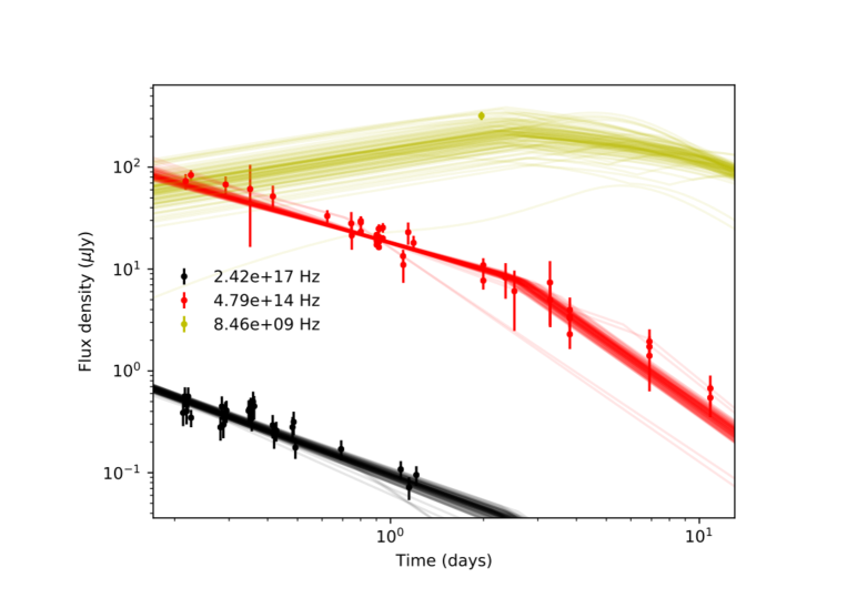
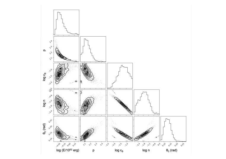
Figure 12: Light curve and corner plot for the fit to GRB 081007 (ISM).

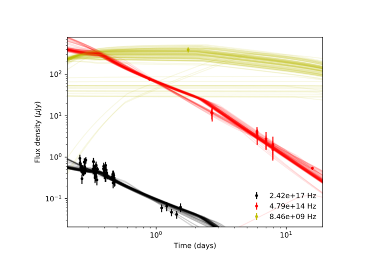
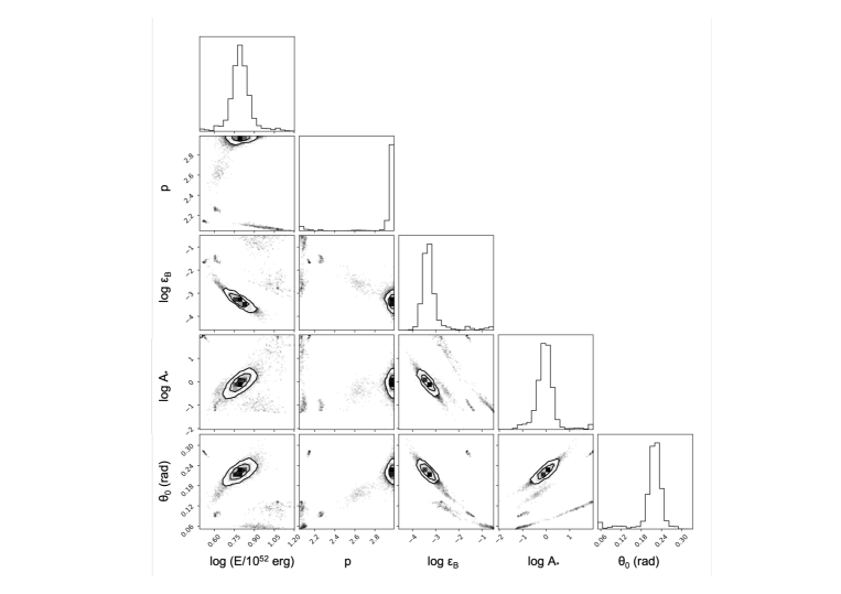
Figure 13: Light curve and corner plot for the fit to GRB 071003 (wind).

Fits were performed on gotohead, the computing cluster of the Gravitational-wave Optical Transient Observer (GOTO) collaboration (Dyer et al., 2020; Gompertz et al., 2020; Steeghs et al., 2022). The full table of results is shown in Table LABEL:app:fits, with some example fits and corner plots in Figures 12 and 13. Fits and corner plots for every burst in the sample are available as supplementary material on the journal website. While the results provide representative sampling of the distributions of GRB afterglow parameters, we caution the reader against over-interpreting individual fits, which are necessarily the product of simplified physical models applied to complex systems (a general problem when fitting models to GRB afterglows). From a sample size of 74, we find a ratio of ISM to wind-like environments of 45/29 = 1.55$\pm$0.37 (Poisson uncertainties). Previous estimates for this ratio are in the range $\sim$1–3, with the precise value likely dependent on sample selection effects and the modelling methods used (Schulze et al., 2011; Gompertz et al., 2018; Zhang et al., 2022).

3 GRB Progenitor Models

To model the CSM of long GRB progenitors, we first need stellar evolution models, with properties such as the mass-loss rate as a function of time. The binary stellar evolution models we use are selected according to the criteria of Chrimes et al. (2020) from BPASS (Binary Population and Spectral Synthesis v2.2.1, Eldridge et al., 2017; Stanway & Eldridge, 2018). The BPASS models explicitly include binary interactions such as mass transfer, and cover the full range of binary parameter space. The models are weighted in metallicity bins, according to their predicted occurrence in a 10⁶ M_⊙ population (based on observations of local stellar populations, Moe & Di Stefano, 2017). In Chrimes et al. (2020), tidal interactions are added to the models in post-processing, and the stellar rotations are tracked.

Two pathways are assumed to produce viable long GRB progenitors. The first is quasi-homogeneous evolution (QHE), where a secondary star ($>20$M_⊙) is spun up by accretion, undergoing increased rotational mixing. This more efficiently burns the hydrogen and helium, and moves the star blue-wards on the Hertzsprung-Russel diagram. If this occurs at low metallicity ($<0.004$ by mass fraction), we assume that the star maintains a high enough spin all the way to core-collapse to be a long GRB progenitor (as line-driven winds and therefore angular momentum loss are low, Yoon et al., 2006).

Alternatively, because GRBs are known to occur in hosts with metallicities higher than 0.2$Z_{\odot}$ (e.g. Graham et al., 2009; Levesque et al., 2010; Elliott et al., 2013; Schady et al., 2015; Michałowski et al., 2018), the possibility of tidally spun-up progenitors in binaries is considered (see e.g. Podsiadlowski et al., 2004; Izzard et al., 2004; Petrovic et al., 2005; Detmers et al., 2008; Bavera et al., 2022; Arcier & Atteia, 2022, for further discussion of the predictions and implications of this progenitor channel). In these cases, tidal interactions with a companion can maintain rotation where mass loss would otherwise spin the star down. The tidal models are selected if,

1. The chemical composition at core-collapse is reflective of type Ic supernovae, i.e. low hydrogen and helium atmospheric abundances,

2. A black hole is produced in the collapse,

3. The surface angular momentum of the star is above a threshold, tuned to reproduce the observed long GRB rate.

The two pathways (QHE and tides) were together able to reproduce both the observed GRB rate (using the metallicity-dependent star formation history of Langer & Norman, 2006), and independently, the metallicity distributions of the hosts (e.g. Palmerio et al., 2019). Assuming rigid rotation (strong core-envelope coupling), the chosen angular momentum threshold also corresponds to specific angular momenta outside the core of $\sim 10^{16}$cm²s^-1, close to the value required by collapsar accretion disc theory (Woosley, 1993; Petrovic et al., 2005).

We use the tide-adjusted models calculated in Chrimes et al. (2020). These include ‘jumps’ between models where tidal interactions modify the orbital period enough that the system orbital parameters are now better represented by a different model at that timestep. However, these model jumps are the exception rather than the norm, occurring in only $\sim$10 per cent of cases, and jumps are typically only to adjacent models in the model grid. Therefore, the mass loss rates as a function of time in the models used are similar (in most cases identical) to the standard BPASS models. Across the redshift range where afterglows can be studied in detail, the tidal pathway (metallicities up to $\sim Z_{\odot}$) contributes a factor of a few more to the total rate than the QHE channel ($Z<0.2Z_{\odot}$). For further details, we refer the reader to Chrimes et al. (2020), and to Eldridge et al. (2019), Tang et al. (2020) and Briel et al. (2022) for further discussions of transient rate calculations with BPASS.

4 Wind Modelling and Bubble Population Synthesis

In this section we calculate, for each progenitor model, the wind termination shock radius and the wind density parameter $A_{\star}$ at a range of ISM densities. This CSM population synthesis is initially performed by application of analytic solutions to the BPASS models outputs. These results are then adjusted in Section 5 based on comparison to a smaller grid of hydrodynamical simulations. This approach avoids the computational cost of running hundreds of detailed simulations, while still benefiting from the improved accuracy they provide. We assume spherical symmetry throughout.

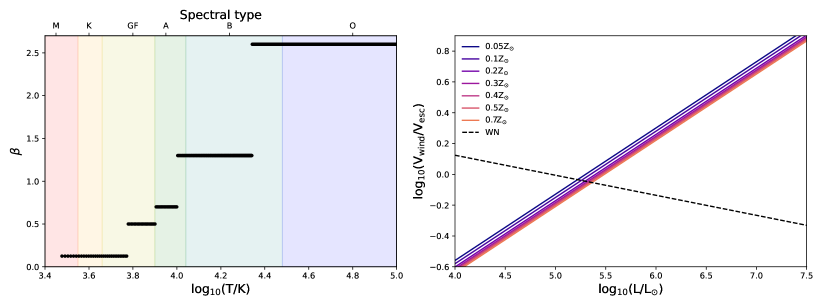
Figure 1: Left: wind speeds in the optically thin regime, where ${\beta}$ is as defined in Equation 1. We use the wind speeds of Eldridge et al. (2006), which are based on results from Hurley et al. (2002), Vink et al. (2001) and Lamers et al. (1995). The speeds calculated from the values shown here are modified by a factor ($Z/Z_{\odot}$)^0.13. The BPASS spectral type definitions are also indicated (Eldridge et al., 2017). Right: optically thick winds (i.e. the Wolf-Rayet regime). We adopt the WC prescription of Nugis & Lamers (2000) for all Wolf-Rayet stars, as this best approximates (out of the WC and WN prescriptions) the results of detailed atmospheric modelling for all Wolf-Rayets (including WC, WO, WN and WNh types, Sander & Vink, 2020), except at the lower luminosity limit of Wolf-Rayet behaviour. The WC winds are shown for a range of metallicities, as is the WN wind (not used) at 0.5 Z_⊙.

4.1 Stellar winds

The BPASS model outputs include every quantity required to calculate wind and wind bubble parameters, except wind velocities. We adopt wind speeds which are similar to those used in the STARS models (Eldridge et al., 2006, on which the BPASS models are built), with some alterations following the results of detailed helium star atmospheric modelling (Sander & Vink, 2020). The BPASS mass loss rates themselves are not altered, as these are part of the stellar evolution models and are included with the model outputs.

4.1.1 Main sequence and pre-Wolf-Rayet

For stars that are not Wolf-Rayets, including those on the main sequence and all phases post-main sequence up to becoming a Wolf-Rayet, we implement a modified version of the wind speeds used by Lamers et al. (1995), Hurley et al. (2002), Vink et al. (2001) and Eldridge et al. (2006). The wind speed in the non-Wolf-Rayet regime is given by,

$$V_{\mathrm{w}}=\sqrt{\beta V_{\mathrm{esc}}^{2}}\times\Big{(}\frac{Z}{Z_{\odot}}\Big{)}^{0.13}$$ (1)

where $Z$ is the metallicity (by mass fraction), and $\beta$ parameterises the wind strength for different effective temperatures. We use the $Z^{0.13}$ metallicity modification of Leitherer et al. (1992) and Vink et al. (2001). The ${\beta}$ values used are shown in the left panel of Figure 1.

The escape velocity at the stellar surface is modelled in the following way. First, a cross-section is defined which depends on the hydrogen and helium atmospheric mass fractions,

$$\sigma_{\mathrm{e}}=0.401\Big{(}X+\frac{Y}{2}+\frac{Y}{4}\Big{)}\,\mathrm{cm}^{2},$$ (2)

which appears in the Eddington factor, along with the mass and luminosity. This accounts for a reduction in effective escape velocity for stars close to the Eddington luminosity L_Edd (i.e., a particle in the wind gets a boost from radiation pressure). The Eddington factor is defined as,

$$\Gamma=\frac{L_{\star}}{L_{\mathrm{Edd}}}=7.66\times 10^{-5}\sigma_{\mathrm{e}}\Big{(}\frac{L_{\star}}{M_{\star}}\Big{)},$$ (3)

and the effective escape velocity is,

$$V_{\mathrm{esc}}=\sqrt{\frac{2GM_{\star}}{R_{\star}}(1-\Gamma)},$$ (4)

where M_⋆ and R_⋆ are the stellar mass and radius respectively.

4.1.2 Wolf-Rayet winds

For Wolf-Rayet stars, we employ the wind velocities of Nugis & Lamers (2000), on which the BPASS v2.2.1 mass loss rates are also based. We identify Wolf-Rayet stars using the standard BPASS definitions (based on temperature and surface abundances, Eldridge et al., 2008, 2017). For WN stars (Wolf-Rayets with nitrogen-rich composition), the wind speed is given by,

$$\mathrm{log}_{10}\Big{(}\frac{V_{\mathrm{wind}}}{V_{\mathrm{esc}}}\Big{)}=0.61-0.13\mathrm{log}_{10}\Big{(}\frac{L_{\star}}{L_{\odot}}\Big{)}+0.30\mathrm{log}_{10}(Y)$$ (5)

where Y is the helium mass fraction. We also have,

$$\mathrm{log}_{10}\Big{(}\frac{V_{\mathrm{wind}}}{V_{\mathrm{esc}}}\Big{)}=-2.37+0.43\mathrm{log}_{10}\Big{(}\frac{L_{\star}}{L_{\odot}}\Big{)}-0.07\mathrm{log}_{10}(Z)$$ (6)

for WC stars (Wolf-Rayets with carbon-rich composition).

These relations are shown in Figure 1. Sander & Vink (2020) studied the mass loss rates and wind speeds of helium stars, with a suite of hydrodynamically consistent atmosphere models. Following the results of Sander & Vink (2020), where log₁₀(L/L_⊙)$\propto$0.3$\times$log₁₀(V_wind/V_esc), we use the Nugis & Lamers (2000) WC prescription for all Wolf-Rayet stars, as this best approximates these next generation atmospheric modelling results. The exception to this is at the (metallicity dependant) lower luminosity limit of Wolf-Rayet behaviour (Shenar et al., 2020).

Figure 2: An example of the analytic solutions of Garcia-Segura & Mac Low (1995a) applied to the BPASS models. A z002-30-0.6-0.6 model is shown (0.1Z_⊙, 30M_⊙ primary, mass ratio of 0.6 and log₁₀(P/days)=0.6) with an ISM density $n=$1 cm^-3. $r_{\mathrm{wind}}$ here is the innermost bubble radius - when the Wolf-Rayet phase starts at ${\sim}$0.1 Myr before core-collapse, the radius works back up from 0. We show evolution in the HR diagram (stellar temperature versus luminosity, top left), wind termination shock radius (top right), mass loss rate (bottom left) and wind speed (bottom right) as a function of time until core-collapse (CC, not exact since the BPASS models stop at the end of core carbon burning). The mechanical wind luminosity at late times, given by Equation 7, is $\sim 5\times 10^{37}$ erg s^-1.

4.2 Analytic bubble prescription and application to BPASS models

Garcia-Segura & Mac Low (1995a) provide analytic solutions for a Wolf-Rayet wind blowing into a main-sequence or supergiant wind. There are two extremes that can be considered: the bubble expansion is driven solely by thermal pressure (as assumed by Weaver et al., 1977), or it is momentum driven (where the shock has cooled). If external pressure from a hot ISM is considered, the problem becomes analytically intractable. Garcia-Segura & Mac Low (1995a) build on the Weaver et al. (1977) model, by considering three distinct wind phases. These are the main sequence, supergiant/LBV, and Wolf-Rayet (corresponding to low density/high velocity, high density/low velocity, and a high density/high velocity wind respectively). Garcia-Segura & Mac Low (1995b) and Garcia-Segura et al. (1996) perform dynamical simulations to check the validity of their analytic solutions, and find that although they do not capture physics such as instabilities in the outflow, the 3-wind model is a good approximation for most massive star evolutionary paths.

At each time-step of the BPASS models, mass loss rate, luminosity, total stellar mass, stellar radius, effective temperature and chemical composition are given as outputs. Wind speeds can be calculated from these parameters as described in the previous section. Working with the thin shell approximation of Weaver et al. (1977), this states that the wind speed is supersonic, the ISM is cold with negligible thermal pressure, and that the shocked wind is adiabatic. The bubble’s expansion is therefore driven by the thermal pressure of the shocked stellar wind (Garcia-Segura & Mac Low, 1995a). The mechanical wind luminosity is given by,

$$L_{\mathrm{w}}=\frac{1}{2}\dot{M_{\mathrm{w}}}V_{\mathrm{w}}^{2},$$ (7)

where a running mean of the mechanical wind luminosity is tracked as the stellar model evolves;

$$\bar{L_{\mathrm{w}}}=\frac{\sum L_{\mathrm{w}}(t<t_{\mathrm{elapsed}})}{t_{\mathrm{elapsed}}}$$ (8)

and the wind termination shock radius at each time step is given by

$$r_{\mathrm{wind}}=\Big{(}\frac{\dot{M_{\mathrm{w}}}V_{\mathrm{w}}}{28}\Big{)}^{\frac{1}{2}}\Big{(}\frac{3850}{\bar{L_{\mathrm{w}}}}\Big{)}^{\frac{1}{5}}t^{\frac{2}{5}}(\pi\rho_{0})^{-\frac{3}{10}},$$ (9)

where $\rho_{0}$ is the ISM density. If the star transitions into a Wolf-Rayet, $r_{\mathrm{wind}}$ resets, and we follow the expansion of the new Wolf-Rayet blown bubble into the CSM produced by the previous phases. An ‘A₀’ quantity is tracked, representing the density of the wind. This quantity is tracked for any post-main sequence, pre-WR phase where the wind is slow and dense. It is defined as,

$$\mathrm{A_{0}}=\rho_{0}r_{0}^{2}=\frac{\dot{M_{\mathrm{0}}}}{4\pi V_{\mathrm{0}}}$$ (10)

and the inner termination shock in this dense wind lies at,

$$r_{\mathrm{wind}}=\Big{(}\frac{\dot{M_{\mathrm{w}}}V_{\mathrm{w}}}{4\pi\times\mathrm{A_{0}}}\Big{)}^{\frac{1}{2}}t$$ (11)

where a time-weighted average of the A₀ parameter since leaving the main sequence is used. The wind density parameter $A_{\star}$ is calculated at each time step and is defined as,

$$A=\frac{\dot{M}}{4\pi V_{w}}=5\times 10^{11}A_{\star}\mathrm{g\,cm^{-3}}$$ (12)

where $A=\rho r^{2}$ (Chevalier & Li, 2000). $A_{\star}$ is a normalisation of the wind density, for $\dot{M}=10^{-5}M_{\odot}$yr^-1 and $V_{w}=1000$kms^-1. If there is no Wolf-Rayet phase, $A=A_{0}$.

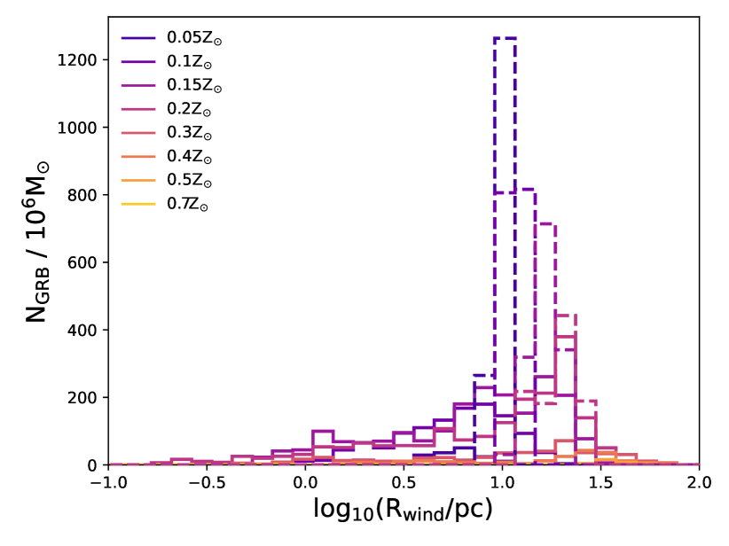
Figure 3: The distribution of final termination shock radii $r_{\mathrm{wind}}$ across all metallicities and models, using the analytic method, at $n=1$ cm^-3. The results are coloured by metallicity. QHE models are shown with dashed lines, tidal pathways with solid lines.

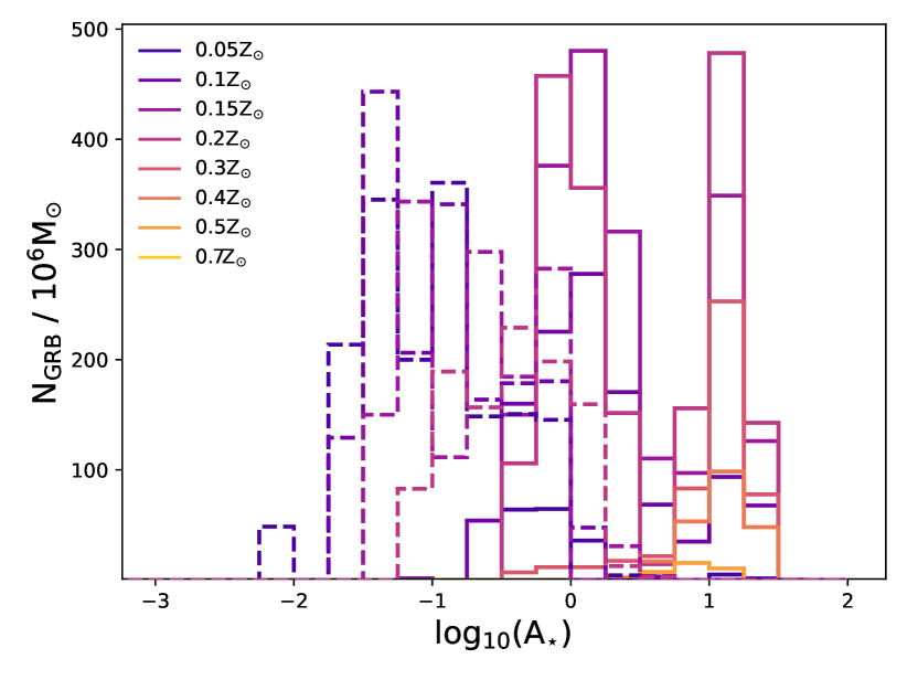
Figure 4: The $A_{\star}$ distribution for all metallicities considered. Tri-modality can be seen, with QHE models (dashed lines) dominating at low $A_{\star}$. The low metallicity models have weaker winds, which would produce smaller bubbles, but this is offset by their longer lifetimes (see Figure 5), giving the bubbles longer to expand. The result is that low metallicity models do not dominate the lowest wind radii (Figure 3). The other two peaks correspond to non-Wolf-Rayet and Wolf-Rayet tidal models.

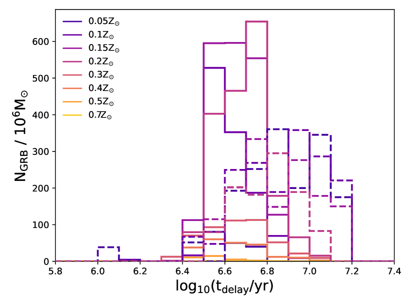
Figure 5: Delay time distributions for the progenitor models. The low-Z QHE models (dashed lines) typically have the longest delay times, while for the non-QHE progenitors (solid lines), higher metallicity models live shorter lives. This is a model selection effect - lower mass and longer lived high $Z$ models typically lose too much angular momentum through winds to be viable long GRB progenitors, assuming strong core-envelope coupling (Chrimes et al., 2020).

We note that the final moments of stellar evolution (post carbon burning, where the BPASS models end) are often marked by rapidly varying mass loss (e.g. Pastorello et al., 2007). This can result in the formation of circumstellar shells. However, because this typically occurs within the final few years of the stellar evolution, such shells have no time to reach the wind termination shock and will be swept away in the initial explosion. We explore this further in the discussion.

4.3 Wind bubble population synthesis

In order to produce predictions for $r_{\mathrm{wind}}$, we run these analytic calculations for every LGRB progenitor model at a range of ISM densities, from $n=10^{-3}$ to $10^{7}$ cm^-3, with order of magnitude steps, for a total of 11 trial densities.

The resultant distributions of $A_{\star}$ and $r_{\mathrm{wind}}$ are weighted by the BPASS weightings, which are informed by the observed distribution of binary parameters in the Galaxy (Moe & Di Stefano, 2017), and a Kroupa IMF up to a maximum mass of 300 M_⊙ (Kroupa, 2001). Since the models have been selected by matching the observed LGRB rate, and the metallicity distribution that arises is comparable to the observed host distribution (the same population for which we have modelled the afterglows in Section 2), no further metallicity weighting is required to match the observed sample.

Our analytic $r_{\mathrm{wind}}$ results are shown in Figure 3 for $n=1$ cm^-3. There is an approximately equal contribution from QHE and binary tidal pathways. The distribution has a strong peak, in part due to the QHE models, for which there are a limited number of BPASS models but which contribute significantly to the rate (resulting in a small number of models, and hence radii and wind densities, being heavily weighted, Eldridge et al., 2017). Furthermore, Equation 11 demonstrates that $r_{\rm wind}$ has a weak dependence on the wind parameters, also decreasing the spread in $r_{\rm wind}$ values.

In Figures 4 and 5 we show the $A_{\star}$ and delay time distributions for the progenitors. Despite QHE stars having the lowest metallicites (and weakest winds), they do not dominate the lowest wind termination radii (Figure 3). This is because they tend to have longer lifetimes (by a few Myr, or a factor of two), as shown in Figure 5, giving more time for bubble expansion. Conversely, the higher metallicity models have shorter lifetimes. This is not intrinsic to the models, but a selection effect: high $Z$ and long-lived stars lose too much mass and angular momentum to be viable long GRB progenitors (Chrimes et al., 2020). As the QHE and low-$Z$ winds are weaker by around a factor of 10 in $A_{\star}$  and the wind radius approximately scales as the square-root of $A_{\star}$  the lifetime differences approximately cancel to yield QHE and low-$Z$ wind radii that are comparable.

5 Exploring the effect of assumptions in the analytic model

5.1 Hydrodynamical simulations

The analytic solutions of Weaver et al. (1977) and Garcia-Segura & Mac Low (1995a) naturally incorporate several assumptions. In order to gain an understanding of how the analytical solutions for $r_{\rm wind}$ found in Section 4 deviate from the results obtained from more physically motivated hydrodynamical simulations, we make use of the PLUTO code (Mignone et al., 2007, 2012; Mignone, 2014). The code solves a system of integrated conservation laws, where the fluid inflow, outflow, temperature and density are tracked in each cell of the simulation. We set up a structured mesh with the ’HD’ module, which uses pure Newtonian hydrodynamics, neglecting magnetic fields and special relativistic effects. The latter is a safe assumption at $\sim$1000kms^-1 wind speeds and temperatures no higher than 10⁵ K, while the lack of magnetic fields is primarily to avoid introducing another variable. Their potential impact is discussed in Section 7.

Our simulations are set up as follows. We use a Runge-Kutta-Legendre (RKL) time-stepping scheme, accurate to second order in time, without dimensional splitting due to our adoption of a cylindrical geometry. Short timescale processes (such as radiative cooling) can then be well approximated, albeit with increased computational cost (see e.g. Townsend, 2009). Cooling is included with an explicit scheme, where the rate of energy loss due to cooling in each cell is proportional to $n^{2}\Lambda(T)$, and we have used the cooling curves of Schure et al. (2009). Full ionisation is assumed above 10,000 K and an ionisation fraction of $10^{-3}$ below. The temperatures in our simulations are typically of this order of magnitude. With cooling included, the stellar wind shock can be radiative, and thermal pressure becomes less important relative to the momentum of the wind. The CFL number is limited to CFL$\leq 0.4$, and a hll Riemann solver is used (Mignone, 2014).

Schure et al. (2009) provide the cooling constant ${\Lambda}$ for Solar metallicity as a function of temperature, and also the contributions from each element at Solar metallicity so that the cooling curve can be adjusted for non-Solar abundances. The curves are scaled by adjusting the contribution from the available elements, according to the relative BPASS abundances at each metallicity (Eldridge et al., 2017). Because not every element calculated by Schure et al. (2009) is available in the BPASS outputs, we only scale the elements that are in BPASS, and keep the others fixed at the Solar value from the fiducial Schure et al. (2009) curve. These are in every case trace elements (e.g. Na, Ar) that do not significantly contribute to cooling. We run the simulations at ZAMS (zero age main sequence) metallicity and do not adjust this throughout the evolution. This is primarily an issue for Wolf-Rayet phases, where the hydrogen abundance of the outflow is reduced, and heavier elements are enhanced. We will discuss the effect of this approximation in Section 7.

To cater for the rare cases where the simulation temperature exceeds the range provided by Schure et al. (2009), we linearly extrapolate the upper end of the curve at each metallicity out to 5${\times}$10⁹ K. This approximates the high temperature, Bremsstrahlung-dominated cooling trends calculated by Ploeckinger & Schaye (2020). We do not employ those curves directly due to significant uncertainties over the exact parameters (e.g. radiation field, dust content) to use, and varying these additional parameters is beyond the scope of this work. We also exclude the effects of dust in our cooling. However, for high-temperature stars at low metallicity, dust formation is likely to be somewhat limited (Everett & Churchwell, 2010). No thermal conduction and a simple ionisation structure are assumed. For detailed study of the effect of these, we refer the reader to e.g. Toalá & Arthur (2011).

Our wind simulation strategy is as follows. A stellar wind with a $r^{-2}$ profile is initialised within a semicircular region of radius 2 pc (8 or 16 cells, depending on the resolution chosen). Given our assumption of spherical symmetry, this yields equivalent results at half the computational cost. The full simulation region is fixed at either $300\times 600$ or $600\times 1200$ cells, with 0.25 pc cell^-1 or 0.125 pc cell^-1. We run the code in a highly parallelised configuration. Unit quantities are chosen to be 1 pc, 1 proton mass per cm³, and 10⁸ cms^-1, with cm, seconds and grams as the units. The unit time step is therefore 970 years. The init.c file used to initialise the simulations is based on the stellar wind example available with PLUTO (Mignone, 2014). The wind is parameterised as ${\rho}\propto Sr^{-2}$, where $S$ is scaled so that the wind has the correct density profile for the given $\dot{M}$, $V_{\mathrm{wind}}$ and simulation units.

The stellar evolution is split into 2-4 phases: main sequence, RSG/YSG/BSG, eruptive episodes (if this occurs and is distinct from other phases) and Wolf-Rayet (if this occurs). The mean mass loss rate and wind velocity are averaged over the duration that the star spends as a specific spectral type (OBAFGKM or Wolf-Rayet), and are used to initialise the simulation wind profile at the start of each stage. The final density, pressure and velocity fields from the previous stage are used as the initial conditions for the next, upon which the new wind profile is superimposed, within 2 pc of the origin, before the simulation is restarted. We are careful not to create scenarios where the superimposed wind in the first stage (when there is no existing simulated bubble, just an ISM) is larger than the expected termination shock radius - this is done by estimating $r_{\mathrm{wind}}$ from the analytic solution.

5.2 Verification of simulations

While the detailed simulations described above contain physics which are not accounted for in the analytic model, if we simulate the conditions assumed in the analytic model, we should obtain a similar result. To test this and verify the reliability of the simulations, we run a 60 M_⊙ single star model at $0.4Z_{\odot}$ for 3.5 Myr, in an $n=100$ cm^-3 (100K) and $n=1$ cm^-3 (8000K) ISM. This model is not selected as a GRB progenitor, but is used here as a standard comparison model with others studied in the literature (e.g. Eldridge et al., 2006; Toalá & Arthur, 2011; van Marle & Keppens, 2012).

The results are shown in Figure 6. In the cold/dense example, the termination shock radius in the simulation is 4.5 pc, versus 4.9 pc from the analytic model. This is expected because the models of Weaver et al. (1977) and Garcia-Segura & Mac Low (1995a) assume (i) an infinitely thin outer shock, and (ii) negligible thermal pressure from the ISM. They also assume no energy loss due to cooling. A dense, cold ISM satisfies criteria (i) and (ii). Aided by our inclusion of radiative cooling in the simulations, which is more efficient at high densities, the outer shock is compressed further.

However, when a hot, low density ISM is used, the assumptions of the analytic model break down - we find 8.7 versus 18.6, a factor of 2.1 difference. The shock is less compressed and has a lower temperature. Since the thermal pressure in the shock and stalled wind must match the wind ram pressure for the bubble to be in equilibrium, and ram pressure decreases with distance from the star, a less compressed outer shock results in a greater radius at which equilibrium is reached, with respect to a model assuming a thin outer shell. Furthermore, if the bubble expands faster than the sound-crossing timescale of the shocked wind, the semi-static assumption of the analytic models also breaks down. Overall, this demonstrates that the analytic method can be inaccurate in ISM temperature and density regimes that are entirely plausible for GRB progenitors.

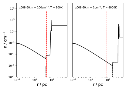
Figure 6: Test simulations performed with PLUTO. In each case, the $r^{-2}$ wind is initialised in a region of radius 2 pc centered at (0,75). The wind parameters are based on a $0.4Z_{\odot}$, $60M_{\odot}$ BPASS model, chosen as the test example for its similarity to simulations performed in the literature (e.g. Eldridge et al., 2006; Toalá & Arthur, 2011; van Marle & Keppens, 2012). The model has a mean main sequence mass loss rate of log₁₀($\dot{M}/M_{\odot}$yr^-1)$=-5.73$ and a mean wind speed of 1740 kms^-1. The simulation is stopped at 3.5 Myr (shortly before the end of the main sequence). The first run uses an ISM density of 100 cm^-3 and a cold ISM of $T=100$K, the second uses 1 cm^-3 and $T=8000$K. The two resultant 1D profiles are shown in the left two panels, and the corresponding 2D density maps on the right. The 1D profiles are drawn from $y=75$ pc. As expected, the dense/cold example reproduces the Weaver et al. (1977) $r_{\rm{wind}}$ prediction well (4.5 versus 4.9 pc), whereas the low density/hot ISM produces 18.6 versus 8.7 pc, a factor of $\sim$2 difference. In the 1D plots, the analytic r_wind values are indicated by dashed vertical red lines, the position of the hydrodynamical termination shocks are noted by shorter dashed black lines.

5.3 Corrections to the analytic results

We used analytic solutions to make a population study feasible in Section 4, as running detailed hydrodynamical simulations for hundreds of models would be unreasonably computationally expensive. However, the more physically motivated simulations yield different results, as shown in the previous section. Since running hydrodynamical simulations for every model is a significant (and perhaps unnecessary) undertaking, we instead consider the application of corrections to the analytic results for $r_{\rm wind}$ to better match hydrosim results. This is done by performing simulations for 16 combinations of progenitor model and ISM density, as listed in Table 2, calculating the factor increase in $r_{\rm wind}$ in the simulation over the analytic result, and finding trends in this increase such that a representative correction can be applied to any given analytic result.

Table 2: Models for which have performed hydrodynamical simulations. The first two are z002-50-0.6-0.6 (0.1Z_⊙, 50 M_⊙ primary, 0.6 mass ratio and log₁₀(P/days)$=0.6$) and z004-50hmg (a 50 M_⊙ QHE model at 0.2Z_⊙). These are both evaluated at $n=$ 0.05, 0.1, 1, 10 and 100 cm^-3. A z014-60-0.7-0.7 model is simulated at 0.1, 1 and 10 cm^-3, and a z010-60-0.9-0.0 model at 0.05 and 10 cm^-3. Additionally, a single star 60 M_⊙ model (not a GRB progenitor) is run at 1 cm^-3 for verification purposes (Section 5.2). For each, we list the analytic prediction for the termination shock radius $r_{\rm wind}$ and the hydrosimulation equivalent, the radius of the outer edge of the stalled wind $R_{\rm sw}$, and the average density log${}_{10}(n_{\rm sw})$ across the stalled wind region.

Model	ISM $n$	$R_{\rm{wind,a}}$	$R_{\rm{wind,h}}$	$R_{\rm{sw}}$	log10($n_{\rm{sw}}$)
z002-50-0.6-0.6	1	8.69	21	39.7	-3.93
z002-50-0.6-0.6	0.1	13.77	33	>75	-4.34
z002-50-0.6-0.6	10	5.48	9.7	20	-3.24
z002-50-0.6-0.6	100	3.97	4.06	9	-2.49
z002-50-0.6-0.6	0.05	15.81	54.9	>75	-4.74
z004-50hmg	10	9.69	15.56	28.5	-3.74
z004-50hmg	1	15.36	31.27	52	-4.27
z004-50hmg	0.1	24.34	42.13	>75	-4.53
z004-50hmg	0.05	27.96	52.54	>75	-4.73
z004-50hmg	100	6.11	8.22	14.45	-3.13
z014-60-0.7-0.4	1	7.56	38.9	62	-3.87
z014-60-0.7-0.4	0.1	11.99	63.38	>75	-4.26
z014-60-0.7-0.4	10	3.05	21.8	33.9	-3.38
z010-40-0.9-0	0.05	9.86	63.8	>75	-4.49
z010-40-0.9-0	10	3.42	21.5	33.1	-3.69
z008-60	1	12.27	27.9	43	-3.92

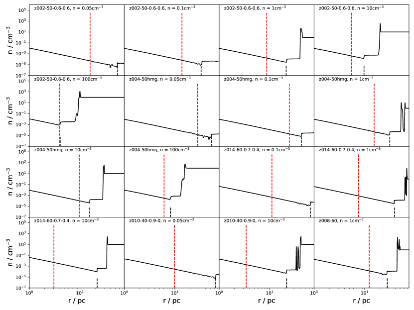
Figure 7: The 16 1D CSM profiles pre-collapse, from simulations that were run in order to (i) compare the result for $r_{\mathrm{wind}}$ to their analytic counterparts and (ii) evaluate the range of stalled wind densities that are possible for a fixed ISM density. The model used and ISM density are indicated in each case, and the results listed in Table 2. The final analytic values for $r_{\mathrm{wind}}$ are indicated by a dashed red lines, the hydrodynamical values by shorter dashed black lines.

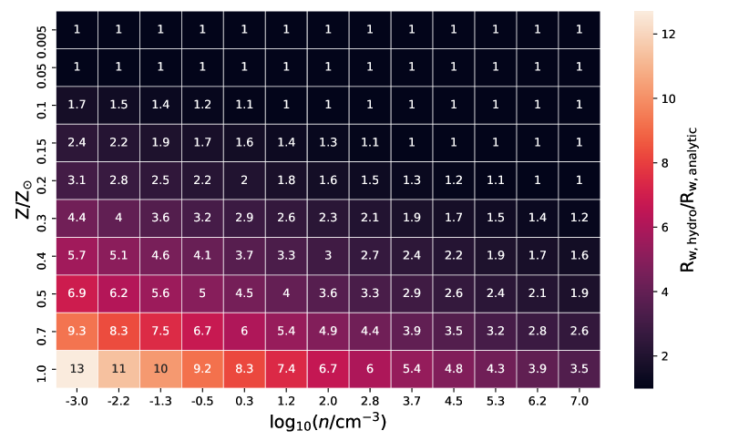
Figure 8: The factor by which $r_{\mathrm{wind}}$ increases in a hydrosimulation, versus the analytic result using the same stellar evolution model. Only a small proportion of the hydrosimulation values in the grid were performed, the gaps were filled by fitting functions and interpolating (see text and hydrosimulation outputs in Figure 7). The corrective factor tends to 1 at low $Z$ and high density, likely because the cooling difference between the approaches is reduced, and a dense ISM better reproduces the thin shell structure assumed in the analytic model. We have floored the corrections at 1.

The resultant 1D density profiles are shown in Figure 7. In each case, the analytic model prediction for $r_{\mathrm{wind}}$ is indicated by a vertical dashed line. The hydro results for $r_{\mathrm{wind}}$ are consistently higher than the analytic results. We assume a priori that the metallicity and ISM density will be important factors in determining the deviation from the analytic $r_{\rm wind}$, since these affect cooling and the compression of the outer shock. Fitting power laws across this $Z$-$n$ parameter space, we find that the factor increase in $r_{\mathrm{wind}}$ over the analytic result can be described by $270n^{-0.056}Z^{0.88}$, where $Z$ is the metallicity by mass fraction and $n$ is the ISM density in cm^-3. For those models which have both analytic and hydrodynamic results, the standard deviation between the corrective factor from this fit and the hydro/wind ratio in each case is 0.4. There is therefore considerable scatter in the relation, but it nevertheless approximates the results that would have been obtained, had we performed simulations for each. The corrections across $Z$-$n$ parameter space are shown in Figure 8, extrapolated down to $10^{-3}$ and up to $10^{7}$ cm^-3. The $r_{\mathrm{wind}}$ corrective factor is floored at 1 (i.e. we never decrease it below the analytic value).

This approach of comparing analytic to hydrodynamical results has been performed before, but not for a whole suite of binary models. Eldridge et al. (2006) ran a selection of numerical simulations to determine the range of $r_{\mathrm{wind}}$ and $A_{\star}$ for Wolf-Rayet stars. They found a typical difference of ${\sim}$0.3 dex between the analytic and numerical results. At $n=1$ cm^-3, we also find modest increases of ${\sim}$0.3 dex at low metallicity. At higher metallicity we find a more significant deviation (a few times greater); this may be due to our inclusion of radiative cooling - more impactful at high metallicity - but not applied in the simulations of Eldridge et al. (2006).

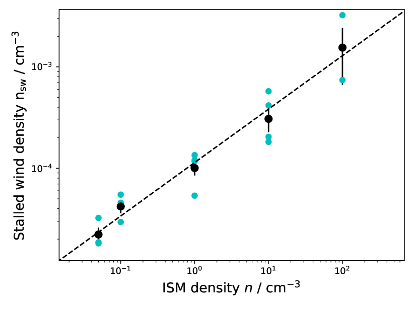
Figure 9: The stalled wind density, for the same models as shown in Figure 7, versus the ISM density. Cyan dots are individual results, larger black dots are means, with the standard error on the mean indicated. Over the range of $n$ simulated, there is a linear relation in log-log space. The stalled wind has a flat density profile and may produce ISM-like afterglow evolution at lower radii than the ISM itself.

A central question is whether the complex shock structure, including a stalled (shocked) wind region beyond $r_{\rm wind}$ but before the ISM, can help explain observations of low constant density media. In addition to correcting the analytic termination shock radius, we also determine the mean outer radius of the stalled wind (i.e. the shock boundary between the stalled wind and ISM) in the hydrosimulations, $r_{\rm ism}$, to be 1.77$\pm$0.07 times the hydrosim termination shock. Within the stalled wind, the densities are approximately constant (see Figure 7), and follow a linear relation in log-log space with the ISM density, as shown in Figure 9. We can therefore select, at 11 hours rest-frame, (i) a wind density $A_{\star}$, for $r_{\rm emit}<r_{\rm wind}$, (ii) a stalled wind density for $r_{\rm wind}<r_{\rm emit}<r_{\rm ism}$ or (iii) the ISM density for $r_{\rm emit}>r_{\rm ism}$. This three-region model approximates most of the CSM simulations well. Hence, starting with analytic $r_{\rm wind}$ and $A_{\star}$ values for each BPASS model and ISM density combination, we can obtain density estimates for the three regions by applying analytic-hydrosim corrections.

To summarise Sections 4 and 5,

• R_wind is obtained for each BPASS model from the analytic estimate (Equations 9 and 11) by multiplying a corrective factor, dependent on metallicity $Z$ and ISM density $n$, as shown in Figure 8,

• the outer stalled wind radius (interface with the ISM) is obtained from a tight $r_{\rm ism}$ = ($1.77\pm 0.07)\times r_{\rm wind}$ relationship,

• the stalled wind density in the region $r_{\rm wind}<r<r_{\rm ism}$ is estimated from an $n$-$n_{\rm ism}$ correlation, demonstrated in Figure 9,

and $A_{\star}$ is a product of the stellar evolution model parameters (Equation 12). All that remains is to decide upon the emission radii with which to sample each model’s CSM, and to generate predictions for a variety of ISM densities.

6 Results

6.1 Observed afterglows

Our full sample of fit results are presented in Table LABEL:app:fits. As noted in Section 2, while we discourage over-interpretation of individual fits, the ensemble can be used to sample the distributions of the physical parameters found in long GRB environments. We find that for ISM-like events, the mean log $(E_{\rm k,iso}/$erg$)=52.99\pm 0.91$, while for wind-like events it’s log $(E_{\rm k,iso}/$erg$)=53.42\pm 0.87$. The finding of a higher average energy for wind-like events is consistent with the results of Gompertz et al. (2018). Indeed, a Kolmogorov-Smirnov (KS) test indicates a probability of $p=0.03$ that the $E_{\rm k,iso}$ values from the two environments were drawn from the same distribution ($p=0.04$ for an Anderson-Darling (AD) test). The significance of this dichotomy is slightly in excess of the $2\sigma$ divide found in Gompertz et al. (2018) and may be due to the factor $\sim 2$ increase in sample size. We also find that $\theta_{o}$ displays a quasi-Maxwellian distribution that peaks at $\theta_{o}\approx 0.1$. Both the KS and AD test find a $p\gg 3\sigma$ separation in $\theta_{o}$ values derived for wind-like and ISM-like environments, but the wind distribution is very broad. Based on a Hellinger distance of $0.03$, we conclude that the wind posteriors for $\theta_{o}$ are just returning the prior. No trends or divisions are observed in $p$ or $\epsilon_{B}$, though $p$ shows a preference for lower values ($p\approx 2$) in both wind-like and ISM-like environments.

6.2 Comparison to the observed Sample

In the previous sections, distributions for $r_{\mathrm{wind}}$ and $A_{\star}$ were produced using an analytic method, and corrections to $r_{\rm wind}$ applied to better match results from hydrodynamical simulations. However, the distributions in Figures 3, 4 and 5 are for all BPASS models identified as possible progenitors. This is not the sample we would see observationally, and is not what should be compared to the results of Section 2. We can only measure $A_{\star}$ in cases where the emission radius $r_{\mathrm{emit}}$ of the GRB jet is inside $r_{\mathrm{wind}}$, and can only measure the stalled wind or ISM densities if the jet has reached that far at the time of observation.

To calculate R_emit for each model at standardised time of 11 hours post-burst (rest frame), we adopt the emission radius-time relations of Pe’er & Waxman (2005) and Gompertz et al. (2018). In a constant density medium (ISM or stalled wind) we have,

$$r_{\rm emit}(t)=5.85\times 10^{17}\bigg{(}\frac{1+z}{2}\bigg{)}^{-\frac{1}{4}}E_{53}^{\frac{1}{4}}n^{-\frac{1}{4}}t^{\frac{1}{4}}$$ (13)

and for a wind-like medium,

$$r_{\rm emit}(t)=3.2\times 10^{17}\bigg{(}\frac{1+z}{2}\bigg{)}^{-\frac{1}{2}}E_{53}^{\frac{1}{2}}A_{\star}^{-\frac{1}{2}}t^{\frac{1}{2}}$$ (14)

where $z$ is the redshift, $E=E_{53}10^{53}$ erg, $n$ is the density in cm^-3, $A_{\star}$ is the wind density parameter and $t_{\rm obs}$ is the rest-frame time post-burst in hours. For each model, we evolve the emission radius from $t=0$ to $t=11$ hours, passing through wind, stalled wind and ISM regions, depending on how far $r_{\rm emit}$ reaches in 11 (rest-frame) hours. Due to the relativistic speeds and assuming small angles with respect to the jet axis, cosmological rest-frame times of 11 hours post-burst can correspond to years of jet propagation. The relation used to model the propagation changes upon crossing the termination shock as outlined above. We note that the precise of choice of 11 hours as the standardised time is somewhat arbitrary, but that the emission radius is only weakly dependent on time as shown above, evolving as t^0.5 or t^0.25.

The wind density parameter is an output from the analytic calculations for a given stellar evolution model, and the ISM density is a pre-chosen value. The density of the stalled wind is calculated with the relation shown in Figure 9. The only variables left in equations 13 and 12 are the redshift and burst energy. We assume a priori that these are not intrinsic to the models or clearly related to the ISM density, so we randomly draw values from the redshift and energy distributions of the observational sample (see Section 2, and Section 7.6 where we investigate the impact of this assumption). We impose a minimum prompt fluence cut for detection of $2\times 10^{-6}$ erg cm^-2, derived from the randomly drawn E_iso and $z$ (luminosity distance, Wright, 2006), based on the conservative lower limit among detected GRBs presented by (Lloyd-Ronning et al., 2019). An efficiency of one is assumed. If the fluence is too low, new E_iso and $z$ pairs are continually drawn until an ‘observable’ fluence is selected. We then move on to the next model and repeat the process. In this way, we populate the observable redshift-flux parameter space.

The only pre-chosen variable is the ISM density. For a choice of ISM density (or range of densities), and for each model (with hydrosim-based corrections applied), an emission radius is generated. Either $A_{\star}$ or $n$ is noted depending on where $r_{\rm emit}$ is at 11 hours, and the CSM structure for that model at core-collapse. In this way, for each choice of ISM density, we can generate synthetic observed distributions of $A_{\star}$ and $n$ using plausible progenitor models and realistic distributions of redshifts and burst energetics.

We list the results of this exercise in the upper part of Table 3. ISM densities from 10^-3 to 10⁷ cm^-3 are trialled. This covers a wide range of environments, from galactic halos to the densest molecular clouds (Ferrière, 2001). To compare to the observed sample, we compare the predicted ratio of ISM to wind-like bursts (observationally 1.55$\pm$0.37, see Section 2), and how well the distribution of $A_{\star}$, $n$ and $r_{\rm emit}$ compare with observations. The KS test p-values from these comparisons are used to gauge how well the distributions match relative to other densities, rather than evaluate a true goodness of fit. This is because we are using fixed ISM densities, with large logarithmic gaps between them, artificially two-step distributions (stalled and ISM densities) in our predictions, which will never agree well with observations. Nevertheless, as the Table 3 shows, it is difficult to get agreement with every observable simultaneously.

We now discuss which is the best single ISM density, based on the statistical comparison of the three distributions ($n$, $A_{\star}$  $r_{\rm emit}$), and the ISM/wind ratio. To evaluate the best-fit log density, for each of $n$, $A_{\star}$  and $r_{\rm emit}$, we calculate the weighted mean density across the range of ISM densities trialled, weighted by the p-value. The resultant weighted mean densities are log₁₀(n/cm^-3)=4.1, –0.9, and 6.6 for $n$, $A_{\star}$  and $r_{\rm emit}$ respectively. The ISM/wind ratio is the only parameter to have a single, clear maximum in probability across this density range, occurring at log₁₀(n/cm^-3)$\sim$3. As this value is also the mean of the three weighted mean densities from $n$, $A_{\star}$  $r_{\rm emit}$, we conclude that $\sim$10³ cm^-3 is overall the best matching single density. The least-well fit parameter is $n$, because at a single ISM density, we only produce two $n$ values (the stalled wind and the ISM itself). To investigate if a range of densities improves this, we also try a Gaussian distribution of log densities, centred at 3. This yields an ISM/wind ratio of 1.08, with $A_{\star}$  and r_wind p-values of –1.37 and –4.67, similar to the $n=1000$ cm^-3 result, while the $n$ p-value is improved as expected, giving $p=-1.77$. The results obtained for this Gaussian distribution of ISM densities are shown in Figure 10.

In Figure 11, we show normalised histograms of the emission radii for both ISM and wind observations, plus ISM and wind-like population synthesis predictions (at $n=1000$ cm^-3). In the predictions, while there is some overlap, emission in ISM environments is strongly biased to higher radii than wind-like environments. However, in the observations, wind-like environments occur out to higher radii than ISM environments. This implies the existence of substantial variety in the wind strengths of the progenitors, ISM densities, or both. Since the maximum of the synthetic $A_{\star}$ distribution is similar to that observed, a population occurring in lower-density environments seems the best explanation for the wind-like environments at large radii. However, when averaged over the population, we find that high density environments are required.

Supernova remnants in the Milky Way favour environments no denser than $n=10$ cm^-3, and typically lower in the Magellanic clouds (Albert & Dwarkadas, 2022), so unless core-collapse GRBs favour denser environments than regular core-collapse supernovae, it is likely that $r_{\rm wind}$ and/or A_⋆ have been overestimated by our population synthesis. The finding that high densities are needed to match the $r_{\rm wind}$ values inferred from GRB afterglows, given otherwise reasonable assumptions regarding the progenitors and mass loss rates, has previously been noted (e.g. Eldridge et al., 2006; van Marle et al., 2006). We have shown this problem to persist at a population level, and now discuss possible explanations for the discrepancy.

Table 3: Synthetic distributions for $A_{\star}$  constant densities (including both the stalled wind region and ISM) and $r_{\rm emit}$ are generated for the following choices of ISM density. The results are compared against the following observables. First, the number of $\sigma$ away from the observed ratio of constant density to wind-like bursts (1.55$\pm$0.37, Poisson uncertainties). Secondly, the distributions of $A_{\star}$  $n$ and $r_{\rm emit}$ through KS tests. The log of the KS test p-value is listed. The null hypothesis that they are drawn from the same distribution is rejected for log₁₀(p)$<-1.3$ ($p<0.05$). In the final row, we list results for a Gaussian distribution in log₁₀(n), centered on 3. Minima in the distributions as a function of density are shown in bold.

log10(n/cm3)	Ratio	$\sigma_{\rm{ratio}}$	$n$ p-val	$r_{\rm emit}$ p-val	$A_{\star}$ p-val
–3	0.04	4.10	–15.7	–5.89	–1.14
–2	0.04	4.10	–13.4	–6.29	–1.13
–1	0.04	4.10	–8.38	–5.78	–1.13
0	0.05	4.07	–3.39	–5.55	–1.15
1	0.12	3.86	–6.50	–5.32	–1.39
2	0.43	3.05	–9.96	–5.65	–1.53
3	1.12	1.18	–8.49	–5.32	–2.08
4	2.69	3.08	–6.64	–5.58	–3.80
5	6.43	13.2	–2.76	–5.18	–6.46
6	11.7	27.5	–5.03	–3.94	–9.61
7	18.9	47.0	–12.2	–3.28	–10.7
Gauss., $\mu=3$	1.08	1.27	–1.77	–4.67	–1.37

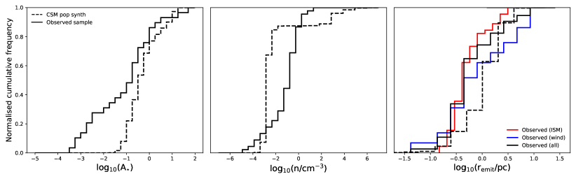
Figure 10: The CSM population synthesis distributions for $A_{\star}$ , $n$ (including stalled wind and ISM contributions) and r_emit versus observations, for a Gaussian distribution in log ISM density, centered at log${}_{10}($n/cm${}^{-3})=3$, the best matching single density with our standard assumptions (see Table 3).

7 Discussion

We now discuss possible explanations for the discrepancy with observation, and whether we can explain the observed CSM variety around long GRB progenitors.

7.1 Radiative cooling

In all 16 simulations used for the analytic corrections (Fig. 7), our cooling was fixed at the initial ZAMS metallicity and not varied. The cooling rate in a Wolf-Rayet wind can be significantly increased, by a factor of 10-100, due to the enhanced abundance of elements heavier than hydrogen, but this does not translate into a large impact in, for example, $r_{\rm wind}$. Mellema & Lundqvist (2002) demonstrate that, with respect to Solar metallicity outflows with the same mass loss rate and velocity, winds from Wolf-Rayet stars produce termination shock radii that are $\sim$1.5 times lower (with significant scatter depending on the exact composition of the wind). However, $\dot{M}$ and $V_{\rm wind}$ can be 10-100 times higher than on the main sequence, which can more than compensate and in some cases dominate over the cooling differences (see equations in Section 4). Finally, we can see in Fig. 6 a simulation which matches the assumptions of the analytic model in every regard, except for the inclusion of cooling. We find $r_{\rm wind}=4.5$ pc (with cooling) versus 4.9 pc (without). Therefore, we conclude that the precise nature of the cooling implemented, or indeed even if it is included or not, is not a dominant factor in driving the CSM structure - particularly as the abundance variation during model evolution applies primarily only to late-stage Wolf-Rayet outflows (if such a phase occurs).

7.2 Binarity

In our simulations, we only included the wind from the progenitor star, without including the companion. The orbital separations are much less than the parsec-scale bubbles, so we can consider the winds from the binary as a single outflow at termination shock distances, even if complex interactions occur on smaller spatial scales (such as colliding winds, Groh et al., 2010). More generally, secondary star winds are typically weaker (secondaries are less massive), and even in the twin case, $\dot{M}$ is only increased by a factor of two. Since $r_{\mathrm{wind}}\propto\sqrt{\dot{M}}$, including the secondary wind would increase $r_{\mathrm{wind}}$ by at most a factor of 1.4 (Equation 11). Another effect of binarity is that the secondary wind, post primary-SN, blows not into the ISM but the wind bubble of the combined primary plus secondary wind up to that point. However, we note that this is only relevant if the system remains bound. For unbound companion velocities of 50 kms^-1, and secondary lifetimes post-primary of 10⁷ yr (Fig. 5), the unbound companion will be $\sim$500 pc away by the time it undergoes core-collapse. Given typical stalled wind-ISM boundary radii of $\sim$1 pc (for a 1 cm^-3 ISM, e.g. Figure 3), this is far outside the sphere of influence of the original system. Since most binary systems are unbound upon primary supernova (e.g. Eldridge et al., 2011; Renzo et al., 2019; Chrimes et al., 2022), the assumption of similar ISM properties for primaries and secondaries should generally hold.

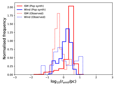
Figure 11: Histograms of the emission radii from both the population synthesis predictions of the best-fit ISM density distribution (solid lines, ISM in red, wind in blue) and observations (dashed lines). The observed sample is more mixed, with wind-like environment found at higher radii than constant density environments. This implies a broader range of progenitor wind strengths and/or densities than simulated.

7.3 Interstellar magnetic fields

Interstellar magnetic fields are not included in the simulations, but also have an effect on the expansion of wind blown bubbles, confining them in the direction perpendicular to the field lines. Although dependent on the field and wind strengths, van Marle et al. (2015) show that the compression along this axis (and resultant decrease in $r_{\mathrm{wind}}$) is typically a factor of a few for magnetic fields of ${\sim}10-20\,{\mu}$G. These field strengths can be found in molecular clouds or close to Galactic centre, but typical Galactic magnetic fields are ${\sim}5\,{\mu}$G (Vallée, 2011).

7.4 Wind bubble asymmetry

Motion through the ISM also has an effect on shock structure, but this is primarily on the outer shock structure, rather than on the inner termination shock at $r_{\mathrm{wind}}$ (e.g., van Marle et al., 2006; Meyer et al., 2020). Furthermore, the compression/rarefaction of the wind bubble is most significant along the direction-of-travel. If the stars with the fastest velocities have been kicked by the supernova of a companion (Cantiello et al., 2007; Eldridge et al., 2011), we might expect them to have been kicked preferentially in the orbital plane, which is typically aligned with the orbital axes. In this case, the jets would tend to be perpendicular to the direction of motion, a direction less affected (on average) by the presence of a bow shock structure. In superbubble environments with hot and tenuous gas, bow shocks may not form at all (Huthoff & Kaper, 2002). Another factor is progenitor rotation, which may lead to asymmetric winds, with the mass loss rate decreased in the polar direction. Since this is the axis along which jets are expected to be launched, if asymmetric mass loss persists until close to core-collapse, the jet may see a termination shock radius a factor of few closer than for spherically symmetric mass loss (Ignace et al., 1996; Eldridge, 2007).

7.5 Eruptive and irregular mass loss

Another consideration is whether eruptive very-late stage mass loss plays a role in shaping the observed afterglow evolution. Such eruptive episodes are thought to produce the dense CSM environments responsible for type IIn supernovae (Smith, 2014). The BPASS models used evolve up to the end of core carbon burning. The neon, oxygen and subsequent core burning stages together last only a few years. Assuming eruptive mass loss with strong winds of 3000 kms^-1 during this time, the furthest any shells ejected post-model is $\sim$0.05 pc (see also Strotjohann et al., 2021). Given that the standardised (cosmological) rest-frame time of 11 hours corresponds to typical jet propagation times and distances post-burst measured in years and parsecs, any impact on the afterglow evolution will be extremely early (in our reference frame) and almost never driving the observed afterglow behaviour. Similarly, late-stage common envelope evolution could eject a large amount of material close to core-collapse. In supernovae with relatively slow moving ejecta, this can influence the lightcurve evolution, for example by producing a bump as the ejecta reaches the previously-ejected common envelope material (e.g. Stevance & Eldridge, 2021). In GRBs however, the jet passage across any region of envelope ejecta will be rapid and unlikely to shape the afterglow evolution in a meaningful way. Finally, it is possible that the stellar wind deviates from an $r^{-2}$ profile at late times, since the rapid evolution of a star could change the stellar wind on a timescale faster than an equilibrium profile can established. This is particularly true for rapidly rotating stars near critical rotation (van Marle et al., 2008). However, such rapid variation is again expected extremely late in the progenitor’s life, and will therefore affect the CSM at very low radii, such that the jet will likely traverse these regions before observations are obtained in our reference frame.

7.6 Correlation between isotropic-equivalent energy and progenitor properties

It is possible that our random assignment of E_iso to each model is missing some correlation between wind properties and burst energy. To investigate, we try drawing initial E_iso values following E${}_{\rm iso}\propto r_{\rm wind}$ and E${}_{\rm iso}\propto 1/r_{\rm wind}$. The first represents the case where more massive stars, with stronger winds, produce stronger GRBs. The second case assumes that stronger winds correlate with weaker bursts (e.g., less angular momentum left in progenitor). In each case, the correlation is parameterised as a log-lin relation (log in E_iso and lin in r_wind), with the maximum E_iso in Section 2 corresponding to the the maximum or minimum r_wind, and vice versa. As in Section 6, we calculate the p-values and ISM/wind ratio at each of the log₁₀(n) values and determine the p-value weighted mean log density, across this range, in each case. Under the assumption that E${}_{\rm iso}\propto r_{\rm wind}$, we find weighted mean log densities of –1.1, 3.4 and 6.9 for $A_{\star}$, $n$ and r_emit respectively. The ISM/wind ratio favours ${\rm n}=100$ cm^-3, with ISM/wind $=1.29$ at this density. The quality of the fits overall is no better than the default random assignment of E_iso, and is worse for r_emit, with typical p-values around log(p)$\sim$–9. For E${}_{\rm iso}\propto 1/r_{\rm wind}$, we find weighted mean log densities of –0.8, 4.5 and 6.3 respectively, with the best ISM/wind $=1.11$ ratio again at ${\rm n}=1000$ cm^-3. Overall, there is no clear indication that the progenitor wind properties are correlated or anti-correlated with E_iso, but on the other hand, this demonstrates that our methodology is robust against assumptions of this nature. We note, however, that we cannot rule out some other correlation with progenitor properties playing a role.

7.7 Mass loss rates and terminal wind velocities

One possibility is that the models selected are not truly representative of the collapsar GRB population. Since we need to decrease the termination shock radius to match observations, and mass loss rates and wind speeds decrease at lower metallicity, we check whether our models are not sufficiently biased to low metallicity by selecting only models at $Z/Z_{\odot}<0.3$. At ${\rm n}=10$ cm^-3, we find an ISM/wind ratio of 0.11, with $A_{\star}$, n, and $r_{\rm{emit}}$ log p-values of –1.38, –5.57 and –7.8 - similar to the results when all metallicities are considered, as in Table 3. The reason for this can be seen in Figs. 3, 4 and 5. Although the lower metallicity models, with include QHE models, have weaker winds, they on average have longer lifetimes. These effects balance, leading to comparable terminal shock radii at the time of core-collapse. Therefore, selecting subsets of our models by metallicity cannot resolve the observed discrepancy.

Alternatively, a reduction in mass loss rates and/or wind speeds more generally may provide a solution. For example, compared to the adopted OB star mass loss rates of Vink et al. (2001), Björklund et al. (2021, 2022) find mass loss rates that are a factor of three lower. There is substantial uncertainty in Wolf-Rayet mass loss rates and wind speeds, and the exact point at which Wolf-Rayet behaviour ceases (Sander et al., 2020; Sander & Vink, 2020). Furthermore, in Fig. 10, we can see that the population synthesis fails to predict the lowest $\sim$third of observed $A_{\star}$ values. Using the analytic approximations in Section 4, for constant wind speeds, $r_{\rm wind}\propto\sqrt{\dot{M_{w}}}$ and vice versa for constant mass loss rates. As an example, for a lower ${\rm n}=10$ cm^-3, artificially reducing $r_{w}$ and $r_{sw}$ by a factor $\sim$three corresponds to late stage mass loss or wind speeds being reduced by a factor of ten. Applying these corrections, we find an ISM/wind ratio of 1.38 ($\sigma_{\rm ratio}=0.48$), and log p-values of –0.73 4.28 and –5.57 for $A_{\star}$, n, and $r_{\rm{emit}}$, overall in better agreement than the default ${\rm n}=10$ cm^-3 results.

7.8 Summary

All of the considerations above could play a role in bridging the gap between observations and modelling, assuming that long GRB progenitors actually explode in lower ISM densities than inferred from our modelling. ISM densities of $100<{\rm n}/$ cm${}^{-3}<1,000,000$ are plausible if core-collapse GRBs occur close to their birth sites in dense molecular clouds (Ferrière, 2001). However, it is expected that the densest cores do not last more than a few Myr (e.g. Vázquez-Semadeni et al., 2005), comparable or shorter than the lifetimes of the progenitors (see Fig. 5). Such dense molecular cloud environments are also expected to be extremely dusty, with high neutral hydrogen column densities, and may also be conducive to producing VHE emission in GRBs (e.g. Rhodes et al., 2022). Given the measured N_H values in GRBs (Evans et al., 2009), prevalence of optically-detected GRBs and rarity of VHE-detected events, qualitatively it appears as though the high densities inferred from our modelling are instead indicative of flaws in the model. Furthermore, our observational sample is biased against dark GRBs, compared with the overall long GRB population (dark fraction $25-40\%$, Fynbo et al., 2009; Greiner et al., 2011), due to the requirement of well-detected optical lightcurves as a pre-requisite. If we favour high density environments for the optically bright GRBs, this implies even higher densities for the overall population, if dark bursts are taken into account. Overall, there is no one factor which can clearly make up the difference between observation and theory. Even for a lower ISM density and reduced wind strengths (as in our ${\rm n}=10$ cm^-3 example above), substantial variation in the termination shock radius is required to reproduce the observed range of wind and ISM environments at different emission radii (Figure 11).

8 Conclusions

In this paper, we have performed a circumstellar medium population synthesis for long GRB progenitors. A semi-analytic wind-blown bubble model was applied to BPASS binary stellar evolution models, to derive termination shock radii where the stellar wind transitions into a flat, shocked wind profile. Through comparison with a grid of hydrodynamical simulations, we derive the outer shocked wind-ISM interface radius for each analytic result, and correct the termination shock radius based on trends in the difference between values derived through analytic and hydrodynamical methods. The results for $r_{\mathrm{wind}}$ and $A_{\star}$ were then compared to the environments, densities and emission radii inferred from the largest long GRB afterglow dataset yet compiled, evaluated at a rest-frame time of 11 hours. We find that, under standard assumptions for the mass loss rates and terminal wind velocities of likely progenitor stars, high ISM densities of ${\rm n}\sim 1000$ cm^-3 best reproduce the observed distributions of $r_{\mathrm{wind}}$ and $A_{\star}$ while also reproducing the observed ratio of ISM to wind-like environments. Given the lack of dark GRBs in our sample, the mean ISM density for the overall population is likely even higher. However, if long GRBs occur in more typical ISM environments (${\rm n}\sim 1$ cm^-3), our predictions for the termination shock radii must be reduced, confirming the findings of individual stellar model studies at a population level. We find that selecting subsets of models by metallicity or the type of progenitor system cannot resolve the discrepancy. Instead, a range of factors from reduced mass loss rates and wind speeds to magnetic field confinement could plausibly be contributing to this persistent gap between GRB observation and theory.

Data Availability

The BPASS binary evolution models used in this work are available via the project website. The post-processed models (as described in Chrimes et al., 2020) and raw data for the CSM population synthesis predictions presented in this paper are available upon reasonable request. The results from the GRB afterglow fitting are available in Appendix LABEL:app:fits, along with example plots showing fits in wind-like and ISM-like media. Equivalent plots for every GRB in the sample are available as supplementary material on the journal website.

Appendix A Afterglow fit results

Table 4: MCMC posterior median values and $1\sigma$ confidence intervals for our sample of GRB afterglows. Our observed sample constitutes 75 GRBs with unique solutions for their environment types. A further 13 GRBs display acceptable fits to either environment. These are tabulated here but not used in our analysis. ISM fits have density units of cm^-3, while wind fits have $5\times 10^{11}$ g cm^-1.

								Radio
GRB	Environment	log(Ek,iso/erg)	p	log($\epsilon_{b}$)	log(n/cm-3)	log(A∗/$5\times 10^{11}$ g cm-1)	$\theta_{o}$ (rad)	data
050315	ism	55.44${}_{-0.37}^{+0.30}$	2.01${}_{-0.002}^{+0.004}$	-4.05${}_{-0.60}^{+0.69}$	-3.34${}_{-0.39}^{+0.45}$	—–	0.02${}_{-0.003}^{+0.006}$	[1]
050318	ism	53.08${}_{-0.36}^{+0.45}$	2.19${}_{-0.09}^{+0.05}$	-3.94${}_{-0.68}^{+1.17}$	0.12${}_{-1.64}^{+1.30}$	—–	0.04${}_{-0.01}^{+0.03}$
050319	ism	54.46${}_{-0.16}^{+0.11}$	2.01${}_{-0.003}^{+0.010}$	-4.30${}_{-0.52}^{+0.69}$	-0.17${}_{-1.07}^{+0.81}$	—–	0.08${}_{-0.02}^{+0.02}$
050416A	ism	54.11${}_{-0.66}^{+0.55}$	2.01${}_{-0.002}^{+0.004}$	-3.74${}_{-0.91}^{+1.12}$	-4.45${}_{-0.38}^{+0.53}$	—–	0.28${}_{-0.15}^{+0.15}$	[1]
050505	wind	53.68${}_{-0.71}^{+0.07}$	2.19${}_{-0.17}^{+0.06}$	-1.15${}_{-0.27}^{+0.37}$	—–	1.77${}_{-0.90}^{+0.18}$	0.30${}_{-0.03}^{+0.11}$
050525A	wind	52.72${}_{-0.49}^{+0.16}$	2.63${}_{-0.53}^{+0.03}$	-4.79${}_{-0.17}^{+3.98}$	—–	-0.17${}_{-0.18}^{+0.44}$	0.43${}_{-0.20}^{+0.05}$	[2,3]
050801	ism	51.49${}_{-0.17}^{+0.23}$	2.10${}_{-0.05}^{+0.53}$	-0.92${}_{-1.14}^{+0.32}$	1.07${}_{-1.71}^{+0.63}$	—–	0.38${}_{-0.13}^{+0.09}$
050802	wind	54.16${}_{-1.11}^{+1.27}$	2.26${}_{-0.15}^{+0.02}$	-2.34${}_{-1.04}^{+1.12}$	—–	-3.17${}_{-0.08}^{+4.08}$	0.27${}_{-0.15}^{+0.16}$
050820A	ism	54.31${}_{-0.10}^{+0.10}$	2.29${}_{-0.01}^{+0.01}$	-4.91${}_{-0.07}^{+0.15}$	-0.48${}_{-0.23}^{+0.21}$	—–	0.13${}_{-0.01}^{+0.01}$	[2,4]
050824	ism	53.17${}_{-0.38}^{+0.37}$	2.00${}_{-0.002}^{+0.005}$	-1.87${}_{-1.15}^{+0.95}$	-1.54${}_{-1.42}^{+1.70}$	—–	0.36${}_{-0.13}^{+0.10}$	[2,5]
050908	ism	52.20${}_{-0.40}^{+0.60}$	2.82${}_{-0.20}^{+0.11}$	-1.46${}_{-0.88}^{+0.67}$	-4.06${}_{-0.58}^{+0.55}$	—–	0.27${}_{-0.16}^{+0.16}$
050922C	ism	53.21${}_{-0.3}^{+0.41}$	2.75${}_{-0.02}^{+0.02}$	-4.53${}_{-0.35}^{+0.84}$	-0.64${}_{-1.51}^{+0.83}$	—–	0.10${}_{-0.04}^{+0.04}$	[2]
060124	wind	53.51${}_{-0.01}^{+0.01}$	2.33${}_{-0.01}^{+0.01}$	-0.51${}_{-0.02}^{+0.01}$	—–	-2.70${}_{-0.01}^{+0.02}$	0.29${}_{-0.13}^{+0.15}$
060418	wind	54.01${}_{-0.91}^{+0.56}$	2.08${}_{-0.03}^{+0.04}$	-4.16${}_{-0.62}^{+2.03}$	—–	-0.39${}_{-0.41}^{+0.35}$	0.19${}_{-0.05}^{+0.07}$	[2,6]
060512	ism	50.86${}_{-0.14}^{+0.39}$	2.13${}_{-0.09}^{+0.12}$	-1.09${}_{-0.61}^{+0.43}$	-1.02${}_{-0.65}^{+0.90}$	—–	0.41${}_{-0.09}^{+0.06}$
060526	ism	52.83${}_{-0.10}^{+0.08}$	2.26${}_{-0.01}^{+0.01}$	-2.88${}_{-1.00}^{+1.08}$	-0.10${}_{-1.27}^{+1.43}$	—–	0.10${}_{-0.04}^{+0.05}$
060607A	wind	53.49${}_{-0.53}^{+0.76}$	2.96${}_{-0.07}^{+0.03}$	-0.85${}_{-1.53}^{+0.19}$	—–	-2.40${}_{-0.16}^{+0.30}$	0.05${}_{-0.02}^{+0.02}$
060714	ism	53.32${}_{-0.22}^{+0.31}$	2.22${}_{-0.0001}^{+0.0002}$	-4.37${}_{-0.45}^{+0.75}$	-0.51${}_{-0.83}^{+1.04}$	—–	0.07${}_{-0.02}^{+0.03}$
060729	wind	53.86${}_{-0.01}^{+0.01}$	2.01${}_{-0.001}^{+0.001}$	-4.98${}_{-0.01}^{+0.02}$	—–	1.35${}_{-0.01}^{+0.00}$	0.50${}_{-0.001}^{+0.001}$
060904B	ism	51.94${}_{-0.56}^{+1.09}$	2.68${}_{-0.13}^{+0.05}$	-2.41${}_{-1.38}^{+1.09}$	-3.01${}_{-1.31}^{+2.61}$	—–	0.30${}_{-0.15}^{+0.14}$
061007	wind	52.46${}_{-0.10}^{+0.13}$	2.38${}_{-0.11}^{+0.07}$	-3.01${}_{-1.21}^{+1.13}$	—–	-0.72${}_{-0.82}^{+1.02}$	0.34${}_{-0.10}^{+0.11}$
061121	wind	55.76${}_{-0.88}^{+0.18}$	2.00${}_{-0.002}^{+0.18}$	-1.02${}_{-0.81}^{+0.37}$	—–	-2.92${}_{-2.06}^{+2.36}$	0.24${}_{-0.13}^{+0.18}$	[7]
061126	ism	53.18${}_{-0.12}^{+0.24}$	2.04${}_{-0.02}^{+0.03}$	-4.01${}_{-0.72}^{+1.01}$	-0.05${}_{-1.54}^{+1.14}$	—–	0.10${}_{-0.04}^{+0.04}$
070125	ism	54.01${}_{-1.27}^{+0.01}$	2.89${}_{-0.01}^{+0.01}$	-4.99${}_{-0.01}^{+3.28}$	-0.18${}_{-0.73}^{+0.03}$	—–	0.25${}_{-0.01}^{+0.12}$	[8]
071003	wind	52.90${}_{-0.05}^{+0.06}$	2.11${}_{-0.02}^{+0.03}$	-0.58${}_{-0.17}^{+0.06}$	—–	-0.97${}_{-0.09}^{+0.38}$	0.18${}_{-0.01}^{+0.02}$	[9]
071010A	ism	52.14${}_{-0.04}^{+0.04}$	2.18${}_{-0.02}^{+0.02}$	-2.32${}_{-0.35}^{+0.62}$	1.29${}_{-0.93}^{+0.52}$	—–	0.19${}_{-0.04}^{+0.03}$
—–	wind	52.47${}_{-0.08}^{+0.05}$	2.15${}_{-0.02}^{+0.04}$	-3.77${}_{-0.27}^{+0.95}$	—–	1.19${}_{-0.41}^{+0.18}$	0.46${}_{-0.06}^{+0.03}$
071031	ism	52.50${}_{-0.26}^{+1.05}$	2.54${}_{-0.15}^{+0.07}$	-3.60${}_{-0.92}^{+1.21}$	-0.97${}_{-1.40}^{+1.67}$	—–	0.28${}_{-0.15}^{+0.15}$
071112C	ism	52.21${}_{-0.59}^{+1.15}$	2.32${}_{-0.04}^{+0.03}$	-3.05${}_{-1.35}^{+1.58}$	-2.60${}_{-1.58}^{+2.24}$	—–	0.30${}_{-0.15}^{+0.14}$
080210	wind	52.83${}_{-0.19}^{+0.44}$	2.15${}_{-0.10}^{+0.18}$	-2.50${}_{-1.61}^{+1.38}$	—–	-0.57${}_{-1.07}^{+1.15}$	0.34${}_{-0.12}^{+0.11}$
080310	ism	52.80${}_{-0.08}^{+0.07}$	2.40${}_{-0.01}^{+0.01}$	-3.72${}_{-0.73}^{+0.88}$	0.53${}_{-1.24}^{+1.05}$	—–	0.15${}_{-0.04}^{+0.05}$
080319B	ism	53.42${}_{-0.21}^{+0.20}$	2.66${}_{-0.004}^{+0.004}$	-4.80${}_{-0.15}^{+0.34}$	-0.84${}_{-0.48}^{+0.38}$	—–	0.26${}_{-0.05}^{+0.05}$	[10-13]
080413B	ism	53.42${}_{-0.05}^{+0.03}$	2.01${}_{-0.001}^{+0.001}$	-3.37${}_{-0.83}^{+1.07}$	0.34${}_{-1.60}^{+1.24}$	—–	0.15${}_{-0.05}^{+0.06}$
080603A	wind	53.45${}_{-1.03}^{+0.19}$	2.03${}_{-0.01}^{+0.19}$	-0.64${}_{-0.30}^{+0.11}$	—–	-1.49${}_{-0.15}^{+0.32}$	0.12${}_{-0.01}^{+0.16}$	[14]
—–	ism	52.75${}_{-0.18}^{+0.16}$	2.07${}_{-0.02}^{+0.04}$	-0.59${}_{-0.22}^{+0.07}$	-2.11${}_{-0.24}^{+0.41}$	—–	0.06${}_{-0.01}^{+0.02}$	[14]
080605	ism	53.33${}_{-0.22}^{+0.25}$	2.03${}_{-0.01}^{+0.02}$	-2.47${}_{-1.43}^{+1.32}$	-1.27${}_{-1.97}^{+2.14}$	—–	0.28${}_{-0.14}^{+0.14}$
080710	wind	51.94${}_{-0.14}^{+0.98}$	2.48${}_{-0.06}^{+0.05}$	-1.99${}_{-1.29}^{+0.90}$	—–	-1.49${}_{-0.79}^{+1.34}$	0.36${}_{-0.14}^{+0.10}$
—–	ism	52.36${}_{-0.39}^{+0.65}$	2.83${}_{-0.09}^{+0.04}$	-3.89${}_{-0.77}^{+1.28}$	-0.27${}_{-1.68}^{+1.41}$	—–	0.15${}_{-0.07}^{+0.09}$
080721	wind	55.21${}_{-0.52}^{+0.50}$	2.21${}_{-0.01}^{+0.02}$	-3.53${}_{-0.97}^{+1.01}$	—–	-1.89${}_{-0.76}^{+0.79}$	0.27${}_{-0.14}^{+0.15}$
080916C	wind	54.32${}_{-0.74}^{+1.07}$	2.32${}_{-0.07}^{+0.06}$	-2.71${}_{-1.46}^{+1.27}$	—–	-2.28${}_{-1.05}^{+1.46}$	0.29${}_{-0.15}^{+0.13}$
080928	wind	52.73${}_{-0.23}^{+0.2}$	2.34${}_{-0.18}^{+0.66}$	-4.50${}_{-0.44}^{+2.82}$	—–	0.14${}_{-0.74}^{+0.67}$	0.28${}_{-0.14}^{+0.15}$
—–	ism	52.33${}_{-0.15}^{+0.51}$	2.23${}_{-0.10}^{+0.12}$	-2.11${}_{-0.86}^{+1.05}$	0.64${}_{-1.60}^{+1.09}$	—–	0.06${}_{-0.02}^{+0.04}$
081007	ism	51.77${}_{-0.08}^{+0.13}$	2.14${}_{-0.05}^{+0.07}$	-1.23${}_{-0.41}^{+0.42}$	-1.73${}_{-0.60}^{+0.55}$	—–	0.13${}_{-0.02}^{+0.03}$	[15]
081008	wind	52.99${}_{-0.18}^{+0.08}$	2.16${}_{-0.02}^{+0.14}$	-2.36${}_{-1.61}^{+1.12}$	—–	-0.97${}_{-0.98}^{+1.46}$	0.33${}_{-0.11}^{+0.11}$
081029	wind	53.59${}_{-0.57}^{+0.37}$	2.08${}_{-0.04}^{+0.22}$	-3.17${}_{-1.14}^{+0.56}$	—–	1.34${}_{-0.79}^{+0.55}$	0.20${}_{-0.03}^{+0.04}$
—–	ism	53.25${}_{-0.32}^{+0.18}$	2.05${}_{-0.02}^{+0.13}$	-1.68${}_{-0.77}^{+0.32}$	1.55${}_{-0.59}^{+0.39}$	—–	0.07${}_{-0.01}^{+0.01}$
090102	wind	55.31${}_{-3.27}^{+0.50}$	2.00${}_{-0.003}^{+0.056}$	-2.61${}_{-1.74}^{+1.47}$	—–	-1.14${}_{-1.61}^{+1.96}$	0.06${}_{-0.03}^{+0.28}$
—–	ism	54.92${}_{-0.56}^{+0.32}$	2.00${}_{-0.002}^{+0.011}$	-4.67${}_{-0.24}^{+0.57}$	-1.77${}_{-0.49}^{+0.68}$	—–	0.02${}_{-0.003}^{+0.013}$
090313	wind	53.76${}_{-0.33}^{+0.03}$	2.03${}_{-0.003}^{+0.098}$	-0.51${}_{-1.04}^{+0.01}$	—–	-0.72${}_{-0.03}^{+0.66}$	0.30${}_{-0.14}^{+0.14}$	[16]
090323	wind	53.68${}_{-0.04}^{+0.03}$	2.78${}_{-0.02}^{+0.01}$	-4.99${}_{-0.01}^{+0.04}$	—–	0.56${}_{-0.04}^{+0.03}$	0.40${}_{-0.06}^{+0.07}$	[17,18]
090328	wind	52.94${}_{-0.20}^{+0.19}$	2.03${}_{-0.01}^{+0.63}$	-3.36${}_{-1.62}^{+2.81}$	—–	0.26${}_{-2.16}^{+0.74}$	0.31${}_{-0.18}^{+0.14}$	[18]
090423	ism	53.90${}_{-0.23}^{+0.24}$	2.19${}_{-0.05}^{+0.05}$	-4.86${}_{-0.10}^{+0.27}$	-0.53${}_{-0.52}^{+0.39}$	—–	0.10${}_{-0.02}^{+0.02}$	[19]
090902B	ism	52.97${}_{-0.03}^{+0.04}$	2.28${}_{-0.02}^{+0.02}$	-3.07${}_{-0.36}^{+0.29}$	-1.10${}_{-0.42}^{+0.50}$	—–	0.19${}_{-0.02}^{+0.03}$	[18]
090926A	ism	52.95${}_{-0.05}^{+0.04}$	2.98${}_{-0.32}^{+0.01}$	-1.86${}_{-0.69}^{+0.05}$	-2.62${}_{-0.03}^{+2.98}$	—–	0.11${}_{-0.003}^{+0.126}$
—–	wind	53.46${}_{-0.47}^{+0.04}$	2.13${}_{-0.01}^{+0.39}$	-4.45${}_{-0.42}^{+3.95}$	—–	1.40${}_{-3.58}^{+0.31}$	0.45${}_{-0.15}^{+0.04}$
091018	ism	52.93${}_{-0.71}^{+0.17}$	2.03${}_{-0.01}^{+0.13}$	-3.20${}_{-1.01}^{+0.88}$	0.26${}_{-1.25}^{+1.34}$	—–	0.09${}_{-0.03}^{+0.04}$
—–	wind	53.55${}_{-0.28}^{+0.27}$	2.01${}_{-0.001}^{+0.006}$	-1.53${}_{-1.57}^{+0.05}$	—–	1.67${}_{-0.02}^{+0.20}$	0.21${}_{-0.03}^{+0.04}$
091020	ism	53.68${}_{-0.09}^{+0.09}$	2.57${}_{-0.01}^{+0.01}$	-4.93${}_{-0.05}^{+0.11}$	-0.28${}_{-0.21}^{+0.19}$	—–	0.32${}_{-0.13}^{+0.13}$	[20]
091024	ism	51.49${}_{-0.09}^{+0.17}$	2.67${}_{-0.12}^{+0.23}$	-2.07${}_{-0.73}^{+0.59}$	1.26${}_{-0.66}^{+0.50}$	—–	0.36${}_{-0.08}^{+0.10}$
—–	wind	51.86${}_{-0.06}^{+0.07}$	2.50${}_{-0.04}^{+0.05}$	-2.69${}_{-0.41}^{+0.56}$	—–	0.11${}_{-0.40}^{+0.33}$	0.46${}_{-0.05}^{+0.03}$
091029	ism	53.80${}_{-0.17}^{+0.17}$	2.22${}_{-0.01}^{+0.01}$	-4.68${}_{-0.23}^{+0.40}$	-0.73${}_{-0.35}^{+0.50}$	—–	0.06${}_{-0.01}^{+0.01}$
091208B	wind	52.81${}_{-0.23}^{+0.75}$	2.10${}_{-0.06}^{+0.09}$	-2.51${}_{-1.65}^{+1.34}$	—–	-1.49${}_{-1.22}^{+1.63}$	0.31${}_{-0.18}^{+0.13}$
100219A	wind	51.90${}_{-0.18}^{+2.58}$	2.43${}_{-0.30}^{+0.17}$	-1.75${}_{-1.48}^{+0.59}$	—–	0.16${}_{-1.71}^{+0.38}$	0.44${}_{-0.21}^{+0.05}$
100418A	ism	54.00${}_{-0.06}^{+0.05}$	2.37${}_{-0.003}^{+0.003}$	-4.74${}_{-0.08}^{+0.10}$	-2.00${}_{-0.03}^{+0.02}$	—–	0.49${}_{-0.013}^{+0.004}$	[21]
100621A	ism	52.95${}_{-0.14}^{+0.09}$	2.01${}_{-0.003}^{+0.006}$	-2.62${}_{-0.74}^{+1.13}$	0.47${}_{-1.70}^{+1.10}$	—–	0.16${}_{-0.06}^{+0.06}$
100906A	ism	53.01${}_{-0.25}^{+0.22}$	2.03${}_{-0.01}^{+0.03}$	-2.33${}_{-1.08}^{+0.68}$	-0.51${}_{-0.92}^{+1.61}$	—–	0.06${}_{-0.01}^{+0.03}$	[22,23]
101219B	ism	51.32${}_{-0.04}^{+0.04}$	2.26${}_{-0.01}^{+0.01}$	-1.75${}_{-0.14}^{+0.15}$	-0.58${}_{-0.15}^{+0.14}$	—–	0.45${}_{-0.05}^{+0.04}$	[24]
110205A	wind	52.88${}_{-0.03}^{+0.03}$	2.44${}_{-0.01}^{+0.01}$	-4.20${}_{-0.09}^{+0.12}$	—–	0.07${}_{-0.07}^{+0.06}$	0.24${}_{-0.01}^{+0.01}$	[25,26]
110213A	wind	53.71${}_{-0.51}^{+0.68}$	2.56${}_{-0.03}^{+0.02}$	-3.97${}_{-0.69}^{+0.62}$	—–	-1.15${}_{-0.09}^{+0.27}$	0.13${}_{-0.03}^{+0.04}$
110715A	ism	52.35${}_{-0.02}^{+0.02}$	2.14${}_{-0.01}^{+0.01}$	-0.99${}_{-0.09}^{+0.09}$	-0.78${}_{-0.13}^{+0.11}$	—–	0.18${}_{-0.01}^{+0.01}$	[27]
110726A	ism	51.78${}_{-0.26}^{+0.32}$	2.04${}_{-0.02}^{+0.05}$	-1.60${}_{-0.91}^{+0.77}$	-0.37${}_{-1.16}^{+1.36}$	—–	0.36${}_{-0.12}^{+0.10}$
110918A	wind	53.62${}_{-0.26}^{+0.09}$	2.08${}_{-0.07}^{+0.04}$	-3.53${}_{-1.06}^{+2.38}$	—–	0.66${}_{-0.77}^{+0.56}$	0.29${}_{-0.07}^{+0.12}$
—–	ism	53.61${}_{-0.12}^{+0.13}$	2.05${}_{-0.01}^{+0.02}$	-3.39${}_{-0.92}^{+1.12}$	-0.29${}_{-1.71}^{+1.27}$	—–	0.11${}_{-0.04}^{+0.05}$
111209A	ism	53.10${}_{-0.04}^{+0.04}$	2.02${}_{-0.002}^{+0.002}$	-0.80${}_{-0.09}^{+0.09}$	-3.66${}_{-0.15}^{+0.14}$	—–	0.08${}_{-0.004}^{+0.004}$	[28]
120327A	wind	52.79${}_{-0.08}^{+0.07}$	2.39${}_{-0.08}^{+0.08}$	-1.90${}_{-0.51}^{+0.38}$	—–	-1.53${}_{-0.18}^{+0.27}$	0.28${}_{-0.13}^{+0.15}$
120404A	wind	52.77${}_{-0.23}^{+0.25}$	2.70${}_{-0.30}^{+0.17}$	-4.58${}_{-0.33}^{+1.48}$	—–	-0.28${}_{-0.29}^{+0.30}$	0.21${}_{-0.05}^{+0.17}$	[29]
—–	ism	52.76${}_{-1.01}^{+0.36}$	2.73${}_{-0.26}^{+0.12}$	-4.44${}_{-0.42}^{+2.78}$	0.78${}_{-0.79}^{+0.65}$	—–	0.08${}_{-0.02}^{+0.03}$	[29]
120521C	ism	53.92${}_{-0.29}^{+0.35}$	2.08${}_{-0.06}^{+0.04}$	-4.54${}_{-0.37}^{+2.80}$	-1.36${}_{-1.86}^{+0.67}$	—–	0.29${}_{-0.14}^{+0.14}$	[30]
120729A	wind	52.43${}_{-0.71}^{+1.14}$	2.42${}_{-0.24}^{+0.29}$	-3.16${}_{-1.29}^{+1.54}$	—–	-1.78${}_{-1.51}^{+1.57}$	0.15${}_{-0.08}^{+0.18}$
—–	ism	51.79${}_{-0.40}^{+0.53}$	2.51${}_{-0.31}^{+0.19}$	-3.57${}_{-0.89}^{+1.05}$	0.50${}_{-1.63}^{+1.06}$	—–	0.08${}_{-0.02}^{+0.05}$
120923A	wind	53.35${}_{-1.44}^{+1.56}$	2.74${}_{-0.67}^{+0.19}$	-2.66${}_{-1.50}^{+1.55}$	—–	-3.05${}_{-0.28}^{+2.56}$	0.29${}_{-0.15}^{+0.14}$
121024A	ism	52.82${}_{-0.18}^{+0.17}$	2.13${}_{-0.05}^{+0.28}$	-3.25${}_{-0.69}^{+1.04}$	0.60${}_{-1.70}^{+1.04}$	—–	0.10${}_{-0.04}^{+0.04}$
130215A	wind	52.57${}_{-0.03}^{+1.16}$	2.01${}_{-0.001}^{+0.002}$	-1.76${}_{-0.44}^{+0.50}$	—–	0.02${}_{-0.38}^{+1.88}$	0.45${}_{-0.16}^{+0.04}$
130606A	wind	53.73${}_{-1.51}^{+0.23}$	2.70${}_{-0.04}^{+0.05}$	-4.64${}_{-0.26}^{+2.14}$	—–	-0.27${}_{-0.06}^{+1.87}$	0.32${}_{-0.13}^{+0.17}$	[31,32]
130831A	wind	53.71${}_{-1.00}^{+1.30}$	2.46${}_{-0.42}^{+0.02}$	-3.44${}_{-1.07}^{+1.42}$	—–	-2.61${}_{-0.06}^{+3.14}$	0.27${}_{-0.11}^{+0.15}$
131030A	ism	52.84${}_{-0.05}^{+0.12}$	2.34${}_{-0.03}^{+0.01}$	-1.38${}_{-2.41}^{+0.07}$	-3.65${}_{-0.06}^{+3.85}$	—–	0.05${}_{-0.002}^{+0.114}$
140311A	wind	53.23${}_{-0.10}^{+0.09}$	2.15${}_{-0.03}^{+0.04}$	-1.28${}_{-0.46}^{+0.47}$	—–	-0.43${}_{-0.43}^{+0.40}$	0.34${}_{-0.13}^{+0.11}$	[33]
140419A	wind	54.33${}_{-0.80}^{+1.12}$	2.32${}_{-0.26}^{+0.04}$	-1.12${}_{-1.16}^{+0.53}$	—–	-3.34${}_{-0.06}^{+4.14}$	0.31${}_{-0.18}^{+0.13}$	[34]
140423A	ism	54.00${}_{-0.16}^{+0.15}$	2.10${}_{-0.02}^{+0.02}$	-4.73${}_{-0.19}^{+0.35}$	-0.52${}_{-0.30}^{+0.42}$	—–	0.06${}_{-0.01}^{+0.01}$
140430A	ism	52.77${}_{-0.42}^{+0.95}$	2.45${}_{-0.11}^{+0.03}$	-2.96${}_{-1.39}^{+1.47}$	-2.75${}_{-1.58}^{+2.55}$	—–	0.28${}_{-0.15}^{+0.15}$
140506A	ism	53.83${}_{-0.17}^{+0.33}$	2.00${}_{-0.002}^{+0.002}$	-4.25${}_{-0.24}^{+0.49}$	1.41${}_{-0.95}^{+0.44}$	—–	0.30${}_{-0.09}^{+0.06}$
140515A	ism	53.65${}_{-0.18}^{+0.32}$	2.08${}_{-0.05}^{+0.15}$	-3.43${}_{-0.93}^{+1.31}$	-0.72${}_{-1.95}^{+1.10}$	—–	0.28${}_{-0.15}^{+0.15}$	[35]
140606B	ism	51.51${}_{-0.10}^{+0.19}$	2.11${}_{-0.06}^{+0.05}$	-2.91${}_{-0.91}^{+1.44}$	0.11${}_{-2.10}^{+1.40}$	—–	0.24${}_{-0.11}^{+0.11}$
140629A	ism	52.95${}_{-0.19}^{+0.24}$	2.25${}_{-0.03}^{+0.03}$	-4.45${}_{-0.40}^{+0.63}$	0.24${}_{-0.60}^{+0.77}$	—–	0.07${}_{-0.01}^{+0.02}$
140801A	ism	52.24${}_{-0.15}^{+0.20}$	2.18${}_{-0.02}^{+0.02}$	-3.39${}_{-0.97}^{+1.65}$	-0.16${}_{-2.23}^{+1.55}$	—–	0.23${}_{-0.11}^{+0.13}$
150910A	wind	53.69${}_{-0.83}^{+1.60}$	2.42${}_{-0.25}^{+0.03}$	-2.41${}_{-1.30}^{+1.50}$	—–	-2.85${}_{-0.08}^{+1.56}$	0.29${}_{-0.15}^{+0.13}$
160625B	ism	54.23${}_{-0.12}^{+0.11}$	2.27${}_{-0.001}^{+0.001}$	-4.93${}_{-0.05}^{+0.10}$	-0.90${}_{-0.24}^{+0.28}$	—–	0.17${}_{-0.02}^{+0.02}$	[36,37]
161023A	ism	52.81${}_{-0.05}^{+0.07}$	2.93${}_{-0.01}^{+0.01}$	-2.11${}_{-0.08}^{+0.07}$	-2.01${}_{-0.07}^{+0.07}$	—–	0.08${}_{-0.003}^{+0.003}$
180325A	wind	54.22${}_{-0.35}^{+0.73}$	2.01${}_{-0.001}^{+0.005}$	-2.73${}_{-0.08}^{+0.17}$	—–	1.96${}_{-0.06}^{+0.03}$	0.18${}_{-0.07}^{+0.07}$
—–	ism	52.91${}_{-0.13}^{+0.33}$	2.60${}_{-0.19}^{+0.09}$	-3.95${}_{-0.68}^{+0.94}$	0.37${}_{-1.08}^{+1.05}$	—–	0.08${}_{-0.02}^{+0.03}$
180720B	wind	54.78${}_{-0.24}^{+0.25}$	2.18${}_{-0.01}^{+0.01}$	-4.81${}_{-0.14}^{+0.37}$	—–	-0.59${}_{-0.21}^{+0.18}$	0.33${}_{-0.14}^{+0.12}$	[38]

References

- Aksulu et al. (2022) Aksulu M. D., Wijers R. A. M. J., van Eerten H. J., van der Horst A. J., 2022, MNRAS, 511, 2848
- Albert & Dwarkadas (2022) Albert C., Dwarkadas V. V., 2022, arXiv e-prints, p. arXiv:2205.05103
- Alexander et al. (2016) Alexander K. D., Laskar T., Fong W., Berger E., 2016, GRB Coordinates Network, 19606, 1
- Arcier & Atteia (2022) Arcier B., Atteia J.-L., 2022, arXiv e-prints, p. arXiv:2204.05013
- Astropy Collaboration et al. (2013) Astropy Collaboration et al., 2013, A&A, 558, A33
- Barthelmy et al. (2005) Barthelmy S. D., et al., 2005, Space Sci. Rev., 120, 143
- Bavera et al. (2022) Bavera S. S., et al., 2022, A&A, 657, L8
- Beniamini & van der Horst (2017) Beniamini P., van der Horst A. J., 2017, MNRAS, 472, 3161
- Bennett et al. (2014) Bennett C. L., Larson D., Weiland J. L., Hinshaw G., 2014, ApJ, 794, 135
- Berger (2010) Berger E., 2010, ApJ, 722, 1946
- Berger et al. (2005) Berger E., et al., 2005, ApJ, 634, 501
- Björklund et al. (2021) Björklund R., Sundqvist J. O., Puls J., Najarro F., 2021, A&A, 648, A36
- Björklund et al. (2022) Björklund R., Sundqvist J. O., Singh S. M., Puls J., Najarro F., 2022, arXiv e-prints, p. arXiv:2203.08218
- Blandford & McKee (1976) Blandford R. D., McKee C. F., 1976, Physics of Fluids, 19, 1130
- Briel et al. (2022) Briel M. M., Eldridge J. J., Stanway E. R., Stevance H. F., Chrimes A. A., 2022, MNRAS,
- Burrows et al. (2005) Burrows D. N., et al., 2005, Space Sci. Rev., 120, 165
- Cameron & Frail (2005a) Cameron P. B., Frail D. A., 2005a, GRB Coordinates Network, 3495, 1
- Cameron & Frail (2005b) Cameron P. B., Frail D. A., 2005b, GRB Coordinates Network, 3847, 1
- Cameron & Frail (2005c) Cameron P. B., Frail D. A., 2005c, GRB Coordinates Network, 3875, 1
- Cano et al. (2017) Cano Z., Wang S.-Q., Dai Z.-G., Wu X.-F., 2017, Advances in Astronomy, 2017, 8929054
- Cantiello et al. (2007) Cantiello M., Yoon S. C., Langer N., Livio M., 2007, A&A, 465, L29
- Castro-Tirado et al. (2013) Castro-Tirado A. J., et al., 2013, arXiv e-prints, p. arXiv:1312.5631
- Cenko et al. (2010) Cenko S. B., et al., 2010, ApJ, 711, 641
- Cenko et al. (2011) Cenko S. B., et al., 2011, ApJ, 732, 29
- Chandra & Frail (2006) Chandra P., Frail D. A., 2006, GRB Coordinates Network, 5843, 1
- Chandra & Frail (2007) Chandra P., Frail D. A., 2007, GRB Coordinates Network, 6853, 1
- Chandra & Frail (2012) Chandra P., Frail D. A., 2012, ApJ, 746, 156
- Chandra et al. (2008) Chandra P., et al., 2008, ApJ, 683, 924
- Chandra et al. (2010) Chandra P., et al., 2010, ApJ, 712, L31
- Chandra et al. (2018) Chandra P., Nayana A. J., Bhattacharya D., Cenko S. B., Corsi A., 2018, GRB Coordinates Network, 23073, 1
- Chevalier & Li (2000) Chevalier R. A., Li Z.-Y., 2000, ApJ, 536, 195
- Chevalier et al. (2004) Chevalier R. A., Li Z.-Y., Fransson C., 2004, ApJ, 606, 369
- Chrimes et al. (2020) Chrimes A. A., Stanway E. R., Eldridge J. J., 2020, MNRAS, 491, 3479
- Chrimes et al. (2022) Chrimes A. A., et al., 2022, MNRAS,
- Cordes & Lazio (2002) Cordes J. M., Lazio T. J. W., 2002, arXiv e-prints, pp astro–ph/0207156
- Dai & Lu (2002) Dai Z. G., Lu T., 2002, ApJ, 565, L87
- Dai & Wu (2003) Dai Z. G., Wu X. F., 2003, ApJ, 591, L21
- Detmers et al. (2008) Detmers R. G., Langer N., Podsiadlowski P., Izzard R. G., 2008, A&A, 484, 831
- Dyer et al. (2020) Dyer M. J., et al., 2020, in Society of Photo-Optical Instrumentation Engineers (SPIE) Conference Series. p. 114457G (arXiv:2012.02685), doi:10.1117/12.2561008
- Eldridge (2007) Eldridge J. J., 2007, MNRAS, 377, L29
- Eldridge et al. (2006) Eldridge J. J., Genet F., Daigne F., Mochkovitch R., 2006, MNRAS, 367, 186
- Eldridge et al. (2008) Eldridge J. J., Izzard R. G., Tout C. A., 2008, MNRAS, 384, 1109
- Eldridge et al. (2011) Eldridge J. J., Langer N., Tout C. A., 2011, MNRAS, 414, 3501
- Eldridge et al. (2017) Eldridge J. J., Stanway E. R., Xiao L., McClelland L. A. S., Taylor G., Ng M., Greis S. M. L., Bray J. C., 2017, Publ. Astron. Soc. Australia, 34, e058
- Eldridge et al. (2019) Eldridge J. J., Stanway E. R., Tang P. N., 2019, MNRAS, 482, 870
- Elliott et al. (2013) Elliott J., et al., 2013, A&A, 556, A23
- Evans et al. (2007) Evans P. A., et al., 2007, A&A, 469, 379
- Evans et al. (2009) Evans P. A., et al., 2009, MNRAS, 397, 1177
- Everett & Churchwell (2010) Everett J. E., Churchwell E., 2010, ApJ, 713, 592
- Feng & Dai (2011) Feng S.-Y., Dai Z.-G., 2011, Research in Astronomy and Astrophysics, 11, 1046
- Ferrière (2001) Ferrière K. M., 2001, Reviews of Modern Physics, 73, 1031
- Fong & Berger (2013) Fong W., Berger E., 2013, ApJ, 776, 18
- Foreman-Mackey et al. (2013) Foreman-Mackey D., Hogg D. W., Lang D., Goodman J., 2013, PASP, 125, 306
- Frail (2011) Frail D. A., 2011, GRB Coordinates Network, 11549, 1
- Frail et al. (2001) Frail D. A., et al., 2001, ApJ, 562, L55
- Frail et al. (2009) Frail D. A., Chandra P., Singh T., 2009, GRB Coordinates Network, 1088, 1
- Fruchter et al. (2006) Fruchter A. S., et al., 2006, Nature, 441, 463
- Fryer et al. (2019) Fryer C. L., Lloyd-Ronning N., Wollaeger R., Wiggins B., Miller J., Dolence J., Ryan B., Fields C. E., 2019, European Physical Journal A, 55, 132
- Fynbo et al. (2009) Fynbo J. P. U., et al., 2009, ApJS, 185, 526
- Galama et al. (1998) Galama T. J., et al., 1998, Nature, 395, 670